A Nonintrusive Load Identification Method Based on Improved Gramian Angular Field and ResNet18

Abstract

Image classification methods based on deep learning have been widely used in the study of nonintrusive load identification. However, in the process of encoding the load electrical signals into images, how to fully retain features of the raw data and thus increase the recognizability of loads carried with very similar current signals are still challenging, and the loss of load features will cause the overall accuracy of load identification to decrease. To deal with this problem, this paper proposes a nonintrusive load identification method based on the improved Gramian angular field (iGAF) and ResNet18. In the proposed method, fast Fourier transform is used to calculate the amplitude spectrum and the phase spectrum to reconstruct the pixel matrices of the B channel, G channel, and R channel of generated GAF images so that the color image fused by the three channels contains more information. This improvement to the GAF method enables generated images to retain the amplitude feature and phase feature of the raw data that are usually missed in the general GAF image. ResNet18 is trained with iGAF images for nonintrusive load identification. Experiments are conducted on two private datasets, ESEAD and EMCAD, and two public datasets, PLAID and WHITED. Experimental results suggest that the proposed method performs well on both private and public datasets, achieving overall identification accuracies of 99.545%, 99.375%, 98.964%, and 100% on the four datasets, respectively. In particular, the method demonstrates significant identification effects for loads with similar current waveforms in private datasets.

1. Introduction

Global climate change and the high consumption of fossil energy make “energy saving” an important goal in today’s home energy management. Nonintrusive load monitoring (NILM) is an important part of home energy management by obtaining bus load information from a single measurement point and using algorithms to analyze information about individual devices and customer consumption patterns. NILM was proposed by Hart [1] in the early 20th century. The technology can be divided into four parts: event detection, data processing, load decomposition, and load identification. As the core task of NILM, load identification is implemented with advanced algorithms to accurately identify a category of loads based on human-input features or features extracted from electrical signals. The early research on load identification performance [2,3,4] was usually degraded due to the early hardware and software limitations. Recently, the rapid development of deep learning has provided a new direction for load identification.

Feature extraction and classification are two main components of load identification, and deep learning has been widely used in such fields. The deep neural networks were first used in [5] to solve the problem related to NILM. A rectangular network was constructed by combining the long and short-term memory networks (LSTM) and the denoising autoencoders (DAE). Davies et al. presented an automatic feature learning method by down-sampling high-frequency electrical data into four channels to achieve classification results by using a five-layer convolutional neural network (CNN) [6]. Sequence-to-point, spatial, and channel attention mechanisms were combined in [7] to construct a convolutional block attention model to learn target device features.

The objective of load identification is to categorize the load with the recognition of load electrical signals. The nature of load electrical signals is discretized time-series data. If the time-series data is transformed into an image using some sequence-to-image (seq2img) methods, the load identification problem can be treated as the image classification problem. Voltage–current (V-I) trajectory is commonly used to transform voltage and current data into images [8,9,10]. Voltage is plotted versus current to reflect features of load electrical signals. However, the granularity and color information of images are usually missed in such a method, and features of raw data cannot be fully reflected. The recurrence graph (RG) is another seq2img method. The appliance recognition utilizing the recurrence graph technique and CNN was studied, and the weighted recurrent graph (WRG) generation was presented by given with one-cycle current and voltage in [11]. It was shown that an image-like representation with more values can be produced by the WRG to improve appliance recognition performance. In [12], the adaptive weighted recurrence graph (AWRG) was discussed to solve the problem of hyperparameter tuning. It is shown in [13] that the unthresholded recurrence plots are able to work as feature inputs for a vast range of time series classification problems, and the voltage–current trajectory was transformed into two unthresholded recurrence plots. Then it was classified using a spatial pyramid pooling convolutional neural network in [14]. The recurrence graph is helpful in transforming load electrical signals into images. However, the performance of such a method partly relies on the hyperparameters selection. The quality of the generated images can be affected by the selection of hyperparameters. The Gramian angular field (GAF) and the Markov transition field (MTF) were proposed in [15] for encoding time series as images. The time series was represented in a polar coordinate system, and the Gramian matrix was calculated in GAF. Each element of the Gramian matrix was the cosine summation of angles. The MTF was developed to build the Markov matrix of quantile bins after discretization, and the information of the raw data can be encoded by continuously representing the Markov transformation probability and saving information in the time domain.

The above-mentioned seq2img methods may cause key feature loss of raw data. The overall performance of load identification would consequently be affected. For example, the normalization process of the raw data and the construction of pixel matrices when calculating the Gramian matrix may result in information loss of the amplitude feature and the phase feature. If no compensation is made for such information loss, the generated images will be less recognizable, confusion will be induced, and eventually, lead to the load identification error. Some studies have tried to solve this problem. An improved GAF was introduced in [16] to add the amplitude feature to the generated images by multiplying the Gramian matrix with the mean value of the raw data. Li et al. [17] proposed a time series image coding for current time-frequency multifeature fusion to improve the load identification accuracy by combining the Gramian angular summation field (GASF), Gramian angular difference field (GADF), MTF, and current spectrum. The experimental results on the PLAID and IDOUC datasets showed that the overall identification accuracy was improved to about 99.49% and 99.78%, respectively. Qu et al. [18] constructed 2D load signatures, including building the weighted voltage–current (WVI) trajectory image, MTF image, and current spectral sequence-based GAF (I-GAF) image, then built a residual convolutional neural network with energy-normalization and squeeze-and-excitation blocks (EN-SE-RECNN) to perform electrical appliance recognition tasks and achieved good recognition performance on public datasets. Chen et al. [19], respectively, corresponded three single-channel GAF images to the three channels in RGB color space to construct an RGB image as a load signature. Then, a fine-tuned AlexNet model was constructed for performing classification on the load signatures of various appliance loads. For this research, the load signature is constructed to improve the load identification performance. Yusen Zhang et al. proposed three methods, namely learnable recurrent graph (LRG), learnable Gramian matrix (LGM), and generative graph (GG), to transform the image encoding into a learnable process [20]. They achieved experimental results superior to conventional methods using temporal convolutional networks (TCN) on public datasets. Hwan Kim et al. proposed a temporal bar graph to extract the inherent features from the aggregated power signals for efficient load identification [21]. This method achieved higher F1 scores compared to previous methods on the UK-DALE and Tracebase datasets. However, like what has been discussed, the problem of confusion between similar loads is still not well solved. When the signals demonstrate similarity in shape but differ in amplitude and phase, since the amplitude and phase information are usually lost in the seq2img process, the load identification performance could be degraded. Furthermore, none of the aforementioned research conducted experiments on private datasets, so the applicability of their proposed NILM methods to specific application scenarios also requires further validation.

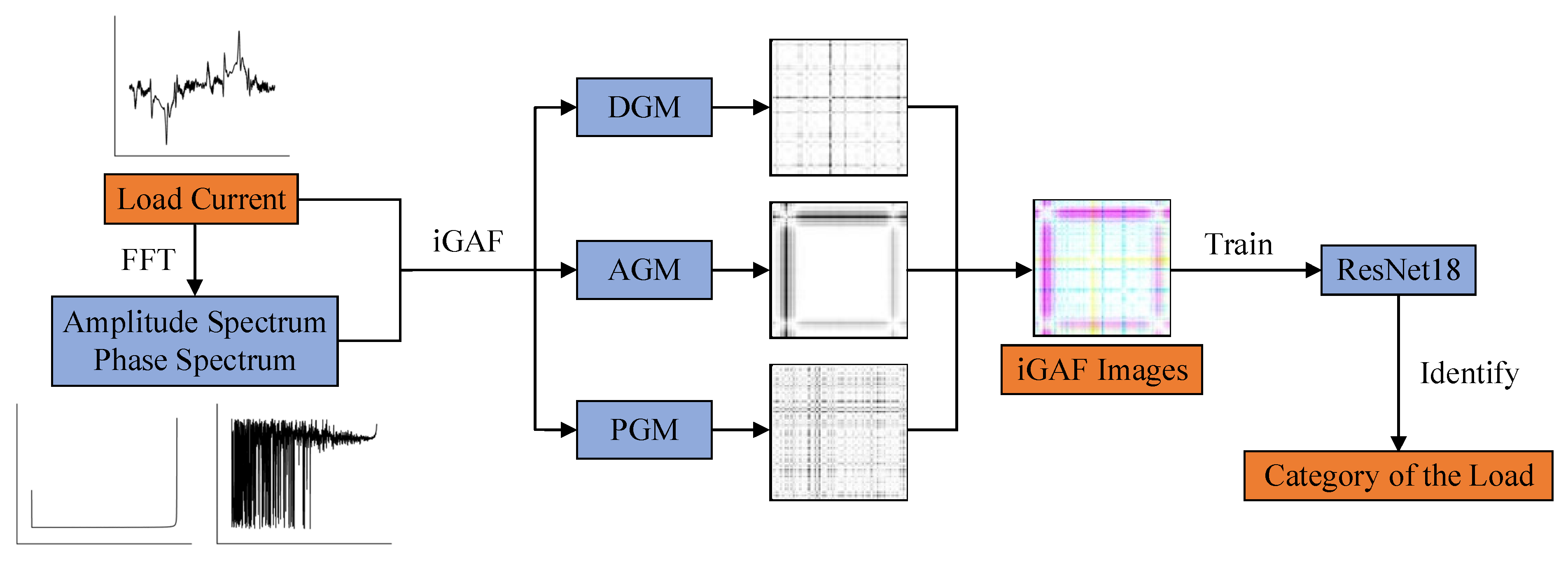
In this paper, a nonintrusive load identification method based on the improved Gramian angular field (iGAF) and ResNet18 is proposed to convert load current signals into improved images to offset the feature loss and thus improve the feature extraction and load identification accuracy. In the proposed method, the amplitude spectrum and phase spectrum of the load current signal are obtained by fast Fourier transform (FFT). The raw data Gramian matrix (DGM), amplitude Gramian matrix (AGM), and phase Gramian matrix (PGM) are, respectively, calculated based on the raw current signal, amplitude spectrum, and phase spectrum. These three matrices are conducted to preserve the amplitude feature and phase feature of the raw data that are usually missed in the existing seq2img methods. Then, the DGM, AGM, and PGM are, respectively, mapped to the three channels of the image to generate the iGAF images, and the ResNet18 is then trained with the iGAF images for load identification. Compared with the images generated by the existing methods, the pixel matrix of each channel of the iGAF image is reconstructed, and the amplitude feature and phase feature of the load current signal can be contained. Loads carrying similar current signals can be more accurately identified by the image classification model trained using iGAF images.

2. Proposed Method

2.1. Overall Scheme of the Improved Gramian Angular Field

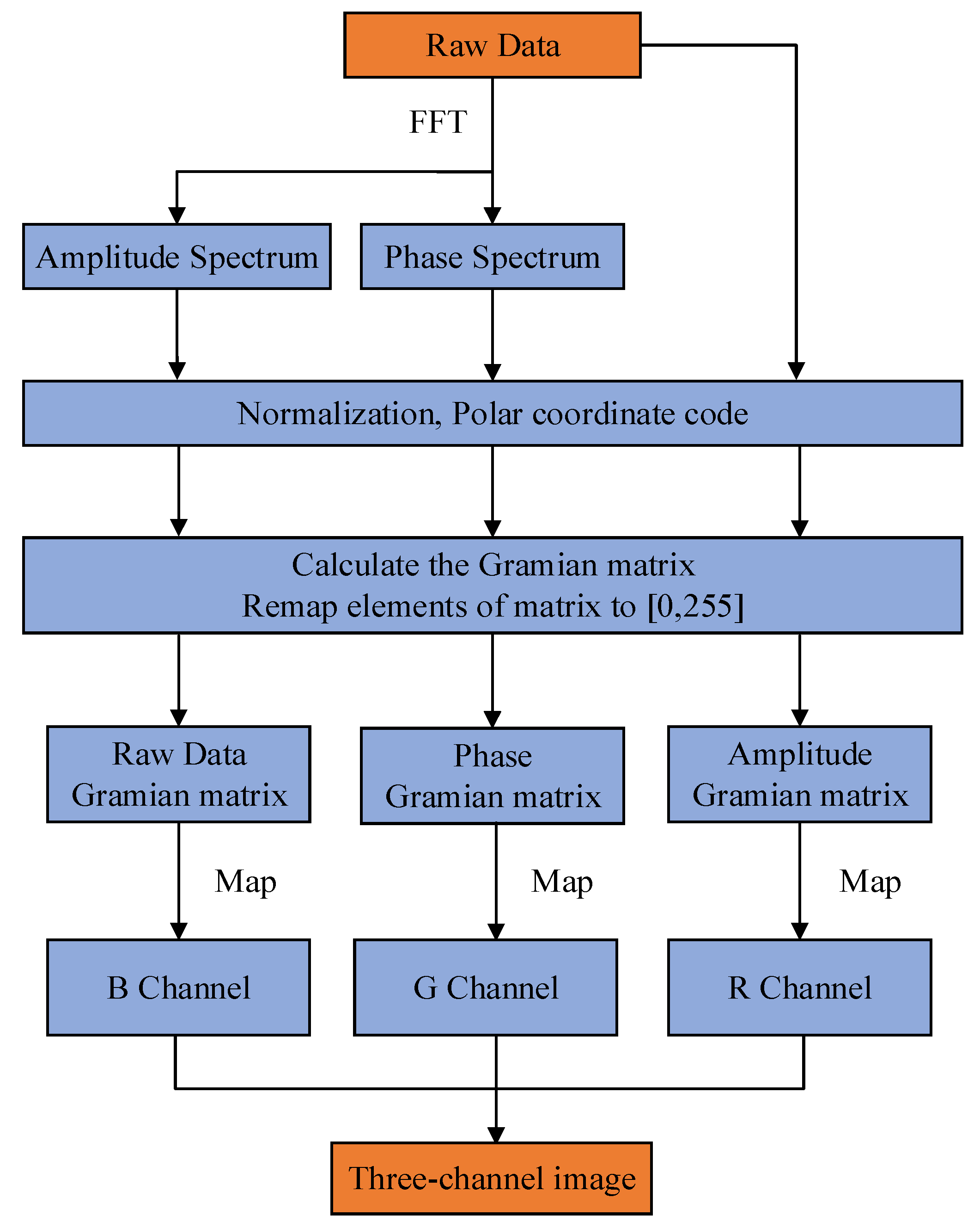
The improved Gramian angular field (iGAF), which is an improved seq2img method, is proposed, and the flowchart is shown in Figure 1. The pixel matrices of the B channel, G channel, and R channel are reconstructed. The amplitude spectrum and phase spectrum of the load current signal are obtained using FFT, after which the DGM, AGM, and PGM are, respectively, calculated based on the load current signal, the amplitude spectrum, and the phase spectrum. Then, the calculated DGM, AGM, and PGM are mapped to the pixel matrices of the B channel, G channel, and R channel. Finally, the three channels are merged into a three-channel image, and thus the amplitude feature and phase feature can be added to the generated iGAF image.

2.2. Calculation of Amplitude Spectrum and Phase Spectrum

The FFT converts signals from the time domain to the frequency domain so that the amplitude, phase, and other information of the signals that are not easily observed in the time domain can be captured in the frequency domain [22,23,24].

Let the raw data be a time-series vector $d=\left[d_1, d_2, \dots , d_n\right]$ with $n$ samples, and FFT is applied to obtain the real part sequence $r=\left[r_1, r_2, \dots , r_n\right]$ and the imaginary part sequence $i=\left[i_1, i_2, \dots , i_n\right]$. The amplitude spectrum $M=\left[m_1, m_2, \dots , m_n\right]$ and the phase spectrum $P=\left[p_1, p_2, \dots , p_n\right]$ are calculated as follows:

$$m_n=\sqrt{r_n^2+i_n^2}$$

(1)

$$p_n={\tan }^{-1}\left(\frac{i_n}{r_n}\right)$$

(2)

2.3. Generation of iGAF Images

Before creating an iGAF representation, a 1D time-series vector X with $n$ samples is normalized to [0, 1] using (3), and the normalized data is converted into polar coordinates [25]:

$${\tilde{x}}_i=\frac{x_i-\min X}{\max X-\min X}$$

(3)

$$\{\begin{array}{c}{\varphi }_i={\cos }^{-1}{\tilde{x}}_i, -1\le {\tilde{x}}_i\le 1, {\tilde{x}}_i\in \tilde{X}\\ r=\frac{t_i}{N}, t_i\in N\end{array}$$

(4)

where $x_i$ is the element of $X$, ${\tilde{x}}_i$ is the element of the normalized time series $\tilde{X}$, ${\varphi }_i$ is the angle of the polar coordinates, $t_i$ is the time stamp, $N$ is the constant to adjust the span of the polar coordinate system, and $r$ is the radius of the polar coordinates.

According to the trigonometric function used, two main types of GAF representations can be generated [15]:

$$G_{DF}=\left[\sin \left({\varphi }_i-{\varphi }_j\right)\right]$$

(5)

$$G_{SM}=\left[\cos \left({\varphi }_i+{\varphi }_j\right)\right]$$

(6)

where $G_{DF}$ and $G_{SM}$ are the two kinds of Gramian matrix; $i, j\in \left[1, n\right]$. The GAF images mainly show the temporal correlation between the pair of data points, along with preserving the temporal and spatial insights. The actual value and angular information have been contained in the main diagonal of the image texture. From (5) and (6), it can be seen that the size of the Gramian matrix is positively correlated with the length of the time series. To reduce the size of the Gramian matrix, piecewise aggregation approximation (PAA) [26] is usually applied to smooth the time series while preserving the trends. The raw data Gramian matrix $G_D$, amplitude Gramian matrix $G_M$, and phase Gramian matrix $G_P$ are defined as follows:

$$G_D=\left[\sin \left({\varphi }_{di}-{\varphi }_{dj}\right)\right]$$

(7)

$$G_M=\left[\sin \left({\varphi }_{mi}-{\varphi }_{mj}\right)\right]$$

(8)

$$G_P=\left[\sin \left({\varphi }_{pi}-{\varphi }_{pj}\right)\right]$$

(9)

where ${\varphi }_d$, ${\varphi }_m$, and ${\varphi }_p$ denote the polar angle converted from each element of the raw data, the amplitude spectrum, and the phase spectrum, respectively. $i, j\in \left[1, n\right]$.

Finally, values in $G_D$, $G_M$, and $G_P$ are remapped to [0, 255] and assigned to the pixel matrices of the B channel, G channel, and R channel, respectively:

$$B=\frac{255}{G_{Dmax}-G_{Dmin}}\times \left(G_D-G_{Dmin}\right)$$

(10)

$$G=\frac{255}{G_{Mmax}-G_{Mmin}}\times \left(G_M-G_{Mmin}\right)$$

(11)

$$R=\frac{255}{G_{Rmax}-G_{Rmin}}\times \left(G_R-G_{Rmin}\right)$$

(12)

where $B$, $G$, and $R$ are the pixel matrices of B channel, G channel, and R channel, respectively. $G_{Dmax}$ is the largest element of matrix $G_D$. $G_{Dmin}$ is the smallest element of $G_D$. Similarly, $G_{Mmax}$ is the largest element of matrix $G_M$. $G_{Mmin}$ is the smallest element of matrix $G_M$. $G_{Pmax}$ is the largest element of matrix $G_P$, and $G_{Pmin}$ is the smallest element of matrix $G_P$.

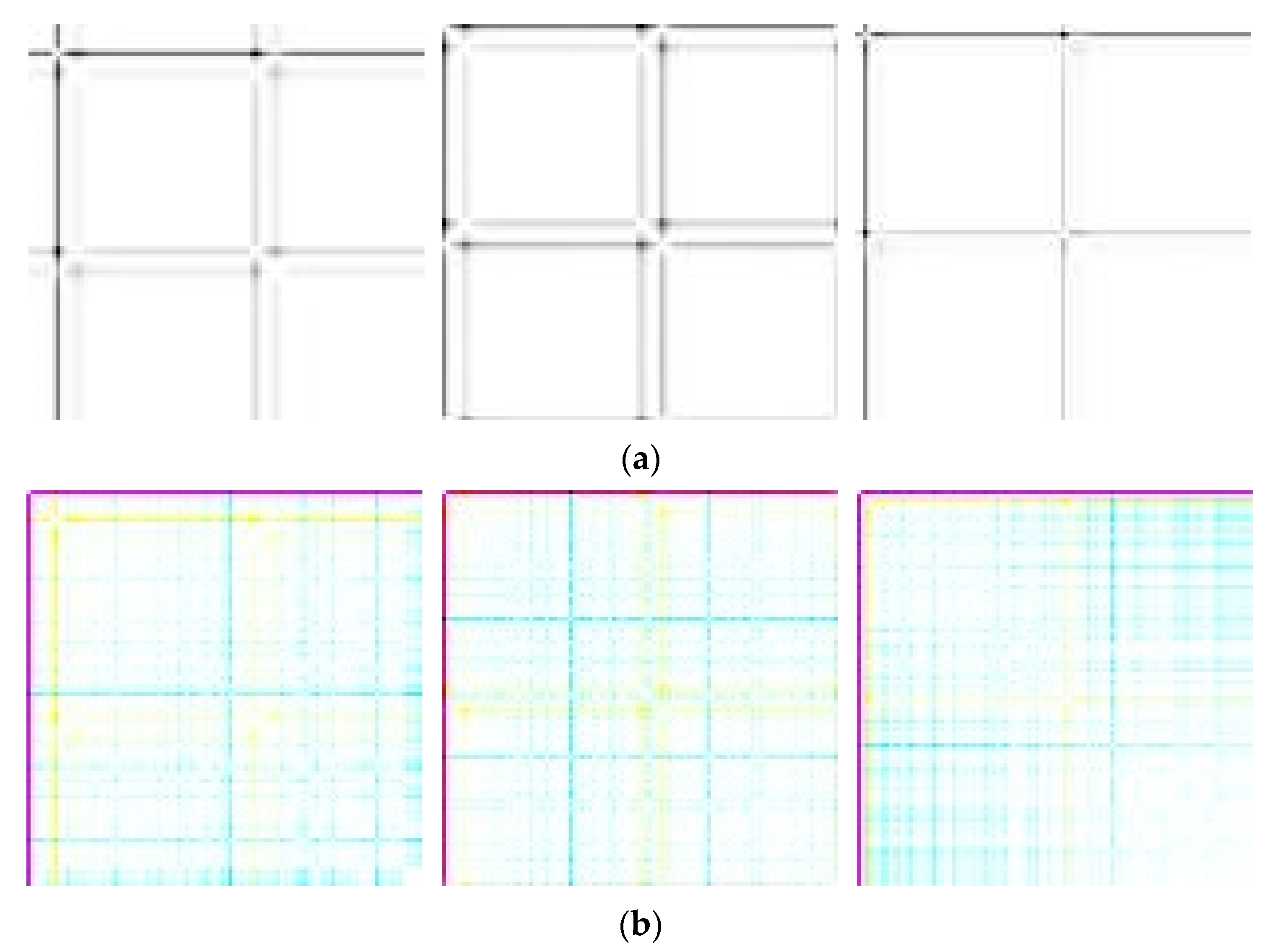
The pixel matrix of the B channel is equivalent to the Gramian matrix in the general GAF, in which the temporal feature of the raw data is contained. The amplitude feature is contained in the pixel matrix of the G channel, and the phase feature is contained in the pixel matrix of the R channel. Finally, by merging the three channels, the iGAF image that combines the temporal feature, the amplitude feature, and the phase feature extracted from the DGM, the AGM, and the PGM, is generated. Here, two sets of images generated by GAF and iGAF are shown in Figure 2 for comparison. It can be seen that the feature differentiation between iGAF images of the three appliances increases.

It is noted that there are six mapping relationships between the three Gramian matrices and the three channels of the image. We use (10), (11), and (12) to demonstrate one of the six. Changing the mapping relationship does not affect the performance of the iGAF method. The six mapping relationships are equivalent.

2.4. Analysis of Feasibility of the iGAF

In the existing GAF, the differences in amplitude between different loads are prevented from being reflected in the generated image by normalization [16]. Additionally, the phase features can be lost because the matrix used to generate images can only reflect the temporal correlation of the raw time series. Moreover, in the existing GAF, only the raw data Gramian matrix is calculated and mapped to the B channel, G channel, and R channel at the same time, which results in equal pixel matrices of the three channels so that the final generated image is grayscale. Color GAF images can be generated by pseudocolor image processing, but the feature information of the load electrical signal contained in it is still only from the raw data Gramian matrix. The features that are lost during the coding will not be offset because of pseudocolor image processing. The absence of the amplitude feature and phase feature is the key reason that the loads that carry similar current signals cannot be accurately identified. It needs to be improved. Combined with the principle of the convolutional layer of CNN, the following analysis is performed.

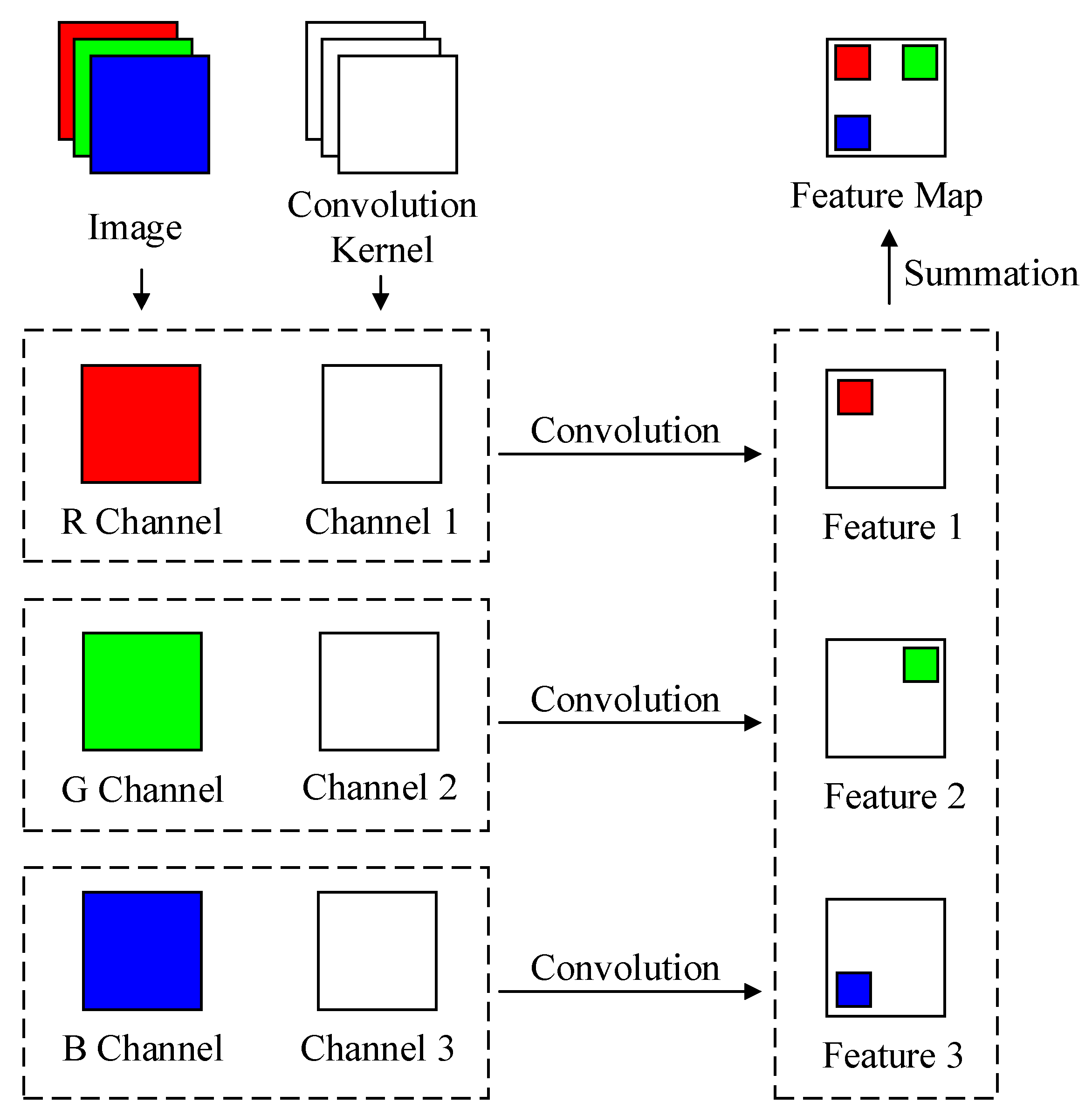
The convolution layer is the core block of a CNN, which consists of a learnable convolution kernel. When the input is a three-channel image, the number of channels of the convolution kernel equals the number of channels of the input image, as shown in Figure 3.

In the feature extraction process, the convolution kernel is divided into three channels to scan the three channels of the image, and the features of each channel are extracted and summarized into one feature map at the end.

For the images generated by the existing GAF, there are three channels. However, the pixel matrices of the three channels are equal, which leads to two problems. First, there is no difference in the features of the three channels. Even if pseudocolor image processing is performed later, the missing amplitude feature and phase feature still cannot be offset. Second, since the pixel matrices of the three channels are equal, the update of the convolution kernel based on the data of three channels in the iterative process is equivalent to the update based on the data of only one channel. In this case, the convolution of a three-channel image using a three-channel convolution kernel is equivalent to the convolution of a single-channel image using a single-channel convolution kernel. The feature extraction capability of the three-channel convolution kernel is not fully utilized, and thus the final performance of identification could be degraded.

However, for the three-channel image generated by the iGAF, the pixel matrices of the three channels are not equal, so the feature information of the three channels is not the same, which greatly increases the recognizability of the generated image. Meanwhile, the feature extraction ability of the three-channel convolutional kernel is fully utilized so that the originally confusing images can be more accurately identified when using the same image classification model.

3. Selection of Image Classification Model and Workflow of the Load Identification

3.1. Image Classification Model

Considering hardware limitations and the feasibility of algorithm deployment in the future, ResNet18 is selected as the image classification algorithm. ResNet has significant structural advantages over other networks. The residual block in the residual network is shown in Figure 4.

As can be seen in Figure 4, the output of the residual block contains the output of the convolutional layer and the identity mapping of the input. The mathematical relationship is shown in (13).

$$H\left(x\right)=F\left(x\right)+x$$

(13)

where $F\left(x\right)$ represents the residual mapping that needs to be learned, $x$ is the input vector, and $H\left(x\right)$ is the output vector.

The addition of the short connection performs a simple constant mapping and forms the basic residual learning units. With the function of the residual block, the degradation problem caused by adding more layers to a suitably deep model can be addressed, and this makes it possible to further increase the number of layers and improve the feature extraction ability of the network. Moreover, it is easier to optimize the residual mapping than to optimize the original, unreferenced mapping, and the shortcut connection introduces neither extra parameters nor computation complexity. Therefore, the training efficiency of the ResNet will be greatly improved on the premise of ensuring the constant expression effect [27,28].

The structural parameters of ResNet18 are illustrated in

Table 1. Parameters for each layer of ResNet18.

Layer	Parameters
conv 1	$7\times 7$, 64, stride 2
conv 2	$3\times 3$ max pool, stride 2 $\left[\begin{array}{cc}3\times 3,& 64\\ 3\times 3,& 64\end{array}\right]\times 2$
conv 3	$\left[\begin{array}{cc}3\times 3,& 128\\ 3\times 3,& 128\end{array}\right]\times 2$
conv 4	$\left[\begin{array}{cc}3\times 3,& 256\\ 3\times 3,& 256\end{array}\right]\times 2$
conv 5	$\left[\begin{array}{cc}3\times 3,& 512\\ 3\times 3,& 512\end{array}\right]\times 2$
Output layer	average pool, fc, softmax

.

For other networks that do not contain residual blocks, adding more layers means that the network degradation and the difficulty of network training increase significantly, so the number of network layers must be reduced appropriately to strike a balance between the difficulty of training and the performance of the network. However, nonintrusive load recognition requires a model with higher accuracy, which requires a deeper structure and higher feature extraction capability of the network. Therefore, conventional CNN cannot meet the requirements of nonintrusive load identification. Combined with the above factors and the computility of our experimental hardware, ResNet18, with structural advantages and lower hardware requirements, is selected.

3.2. Workflow of the Load Identification Based on the iGAF and ResNet18

The diagram of the proposed load identification model based on the improved GAF is shown in Figure 5. The whole workflow of the method is summarized as follows:

• Load current signals are collected, and the arithmetic average filter is applied to the collected data to obtain the raw time-series data.
• FFT is applied to the raw time series data to obtain the amplitude spectrum and phase spectrum.
• If needed, PAA is applied to the raw time series data, amplitude spectrum, and phase spectrum to reduce the length of sequences.
• The Gramian matrices of the raw time series data, the amplitude spectrum, and the phase spectrum are calculated to obtain the DGM, AGM, and PGM.
• Elements in the three matrices are remapped to [0, 255], and the DGM, AGM, and PGM are mapped to the pixel matrices of the B channel, G channel, and R channel, respectively.
• The pixel matrices of the B channel, G channel, and R channel are merged to generate an iGAF image.
• All obtained iGAF images are divided into the training set, the validation set, and the testing set to train ResNet18.
• The trained ResNet18 is used to classify the generated images to obtain categories of loads.

4. Experiments

4.1. Private Datasets

4.1.1. Data Collection

To conduct experimental verifications, the raw electric current signals of eleven different electric appliances and eight different appliance combinations are collected. The categories of loads are shown in

Table 2. Categories of eleven different electric appliances and eight different appliance combinations.

Eleven Single Electric Appliances	Eight Kinds of Appliance Combinations
Induction cooker (standby)	Induction Cooker + Tablet
Induction cooker (running)	Induction cooker + Microwave oven
Desktop	Induction Cooker + Smartphone
Tablet	Microwave + Tablet
Printer	Microwave oven + Smartphone
Coffee Machine	Tablet + Desktop
Microwave oven (running)	Tablet + Smartphone
Microwave oven (standby)	Smartphone + Laptop
Electric soldering iron
Laptop
Smartphone

.

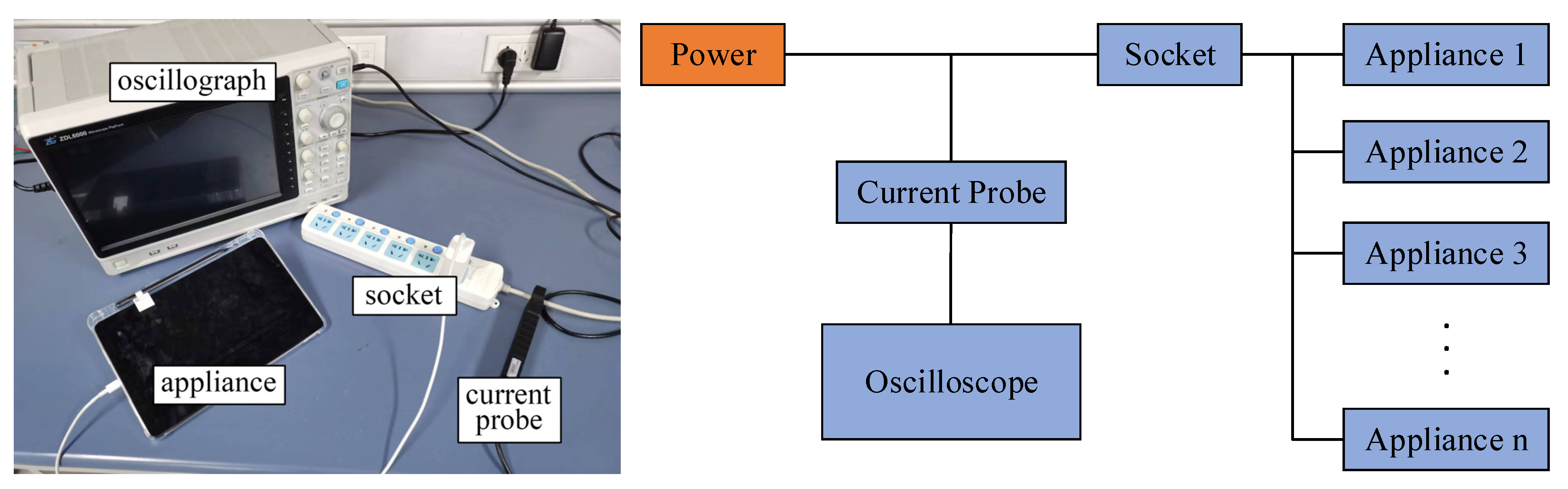
It is seen in Table 2 that the standby and running states of the same appliance are recorded as two categories due to the large difference in currents between the two states. The equipment for data collection and the diagram of the connection are shown in Figure 6. A ZDL6000 oscillograph and a ZCP30 current probe are used for data collection. A 220 V 50 Hz AC power is used for the power supply. The range of the current probe is 30 A. 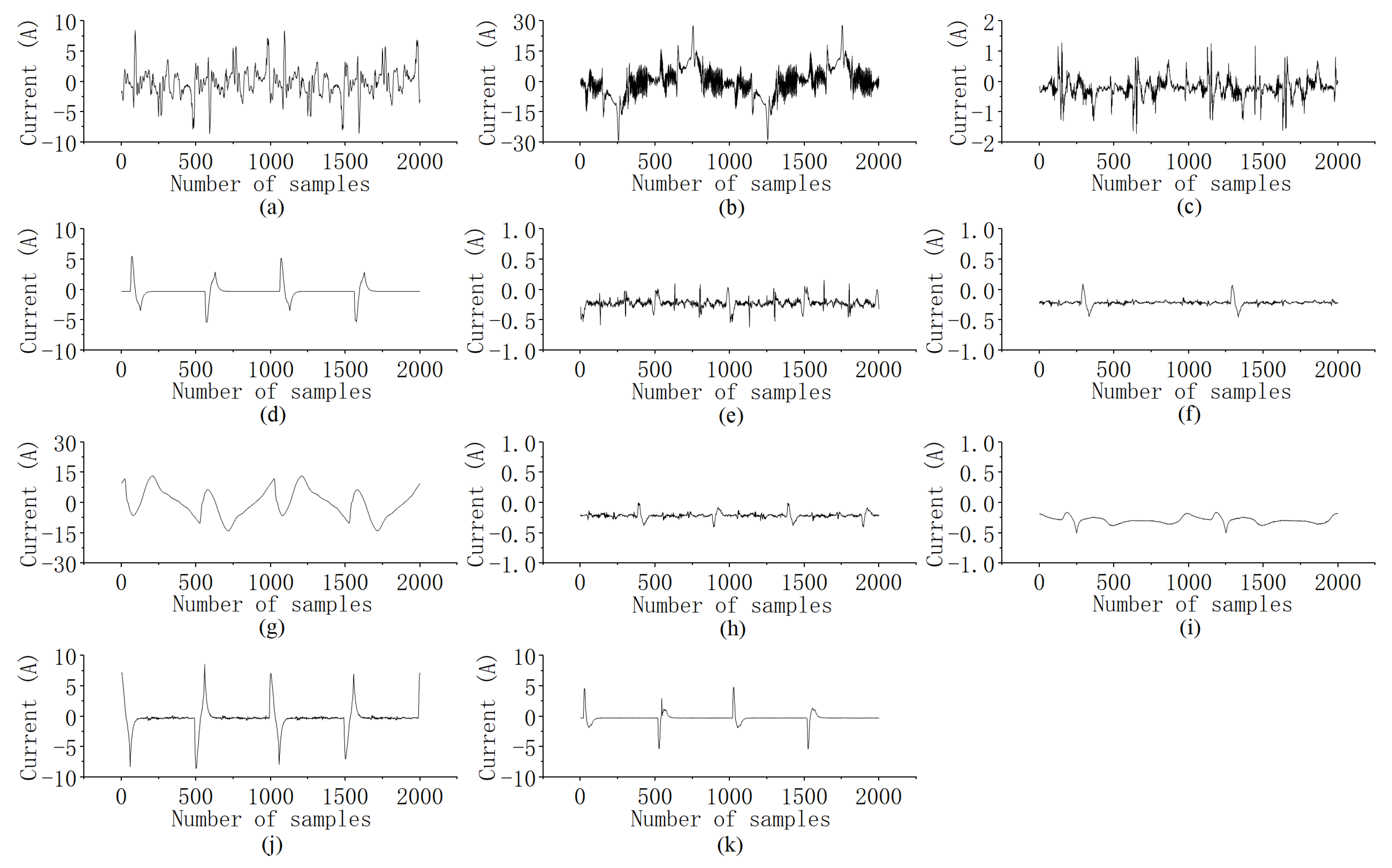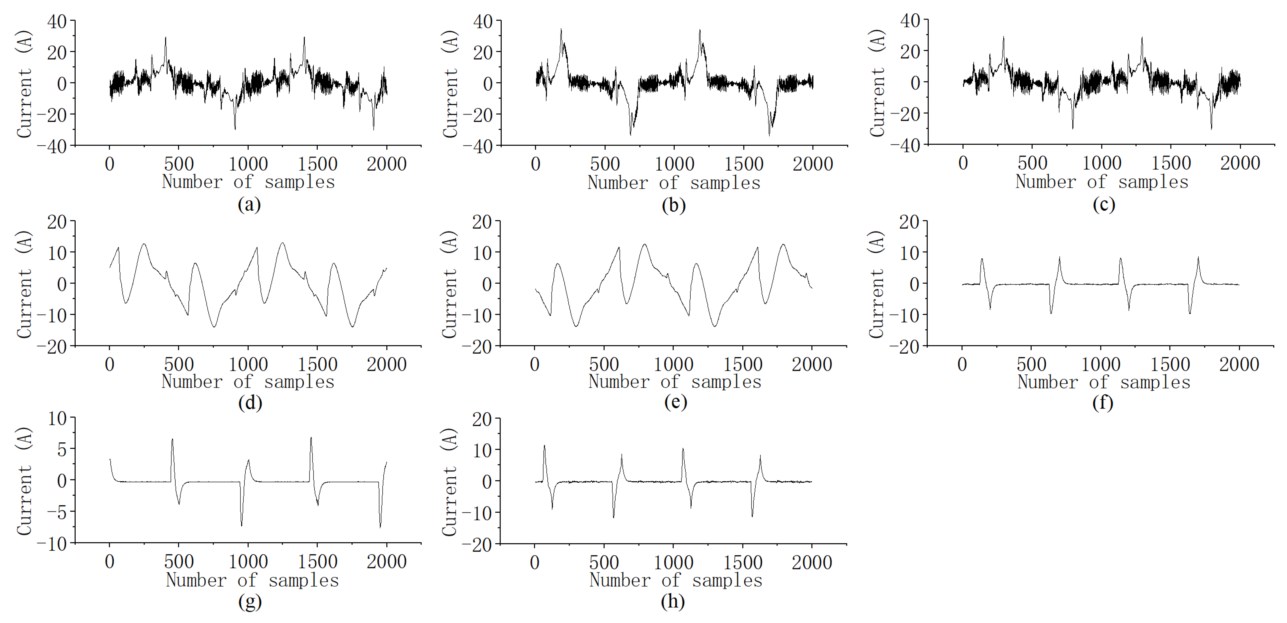It is noted that the sampling frequency should be high enough to avoid aliasing [29] and information loss. Here, the sampling frequency is set as 50 kHz, and the sampling time is 20 s. Collected current waveforms are shown in Figure 7 and Figure 8. Due to the large amount of data, only the first two cycles of each category are shown.

4.1.2. Production of Datasets

Based on the collected current signals in Table 2, two datasets marked as the eleven single electric appliances dataset (ESEAD) and eight mixed-category appliance dataset (EMCAD) are constructed. The ESEAD dataset contains eleven categories of a single appliance. The EMCAD dataset contains four categories of single appliances and four categories of appliance combinations. Furthermore, as shown in

Table 3. Labels for categories in the ESEAD dataset and EMCAD dataset.

Categories in ESEAD	Label	Categories in EMCAD	Label
Induction cooker (standby)	0	Induction cooker + microwave oven	0
Induction cooker (running)	1	Induction Cooker	1
Desktop	2	Desktop	2
Tablet	3	Tablet	3
Printer	4	Microwave + Smartphone	4
Coffee Machine	5	Tablet + Desktop	5
Microwave oven (running)	6	Smartphone + Laptop	6
Microwave oven (standby)	7	Smartphone	7
Electric soldering iron	8
Laptop	9
Smartphone	10

, each category in each dataset is assigned a label.

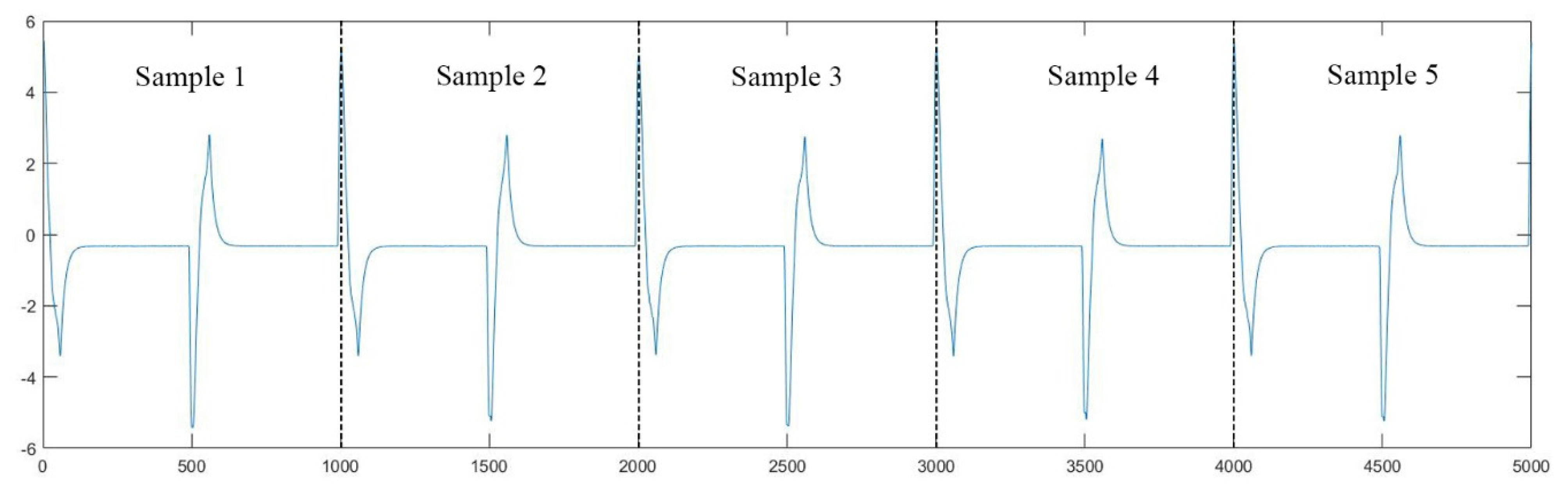
The method for splitting the collected current data to generate samples is as follows. As shown in Figure 9, taking the first five cycles of the waveform of tablet + smartphone, for example, each cycle of the waveform is taken as a sample. For each category, with a sampling frequency of 50 kHz for 20 s, 1 million data points are finally collected, and there are 1000 data points in each cycle of the waveform. Thus, the raw data of each category can be divided into 1000 samples. The total number of samples for ESEAD is 11,000, and the number of samples for EMCAD is 8000. For the training model, each dataset is further divided into the training set, the validation set, and the test set with a ratio of 7:2:1. Each sample in the dataset will be encoded as an image, which is used for training or testing for the model.

4.2. Public Datasets

In addition to the datasets measured and produced by ourselves, two public datasets, namely PLAID [30] and WHITED [31], are used to validate the proposed method. The PLAID dataset includes current and voltage measurements sampled at 30 kHz from 11 different appliance types present in more than 60 households in Pittsburgh, Pennsylvania, USA. The WHITED dataset is derived from 54 types of electrical appliances in 9 regions of the world, including 1339 instances, and the sampling frequency is 44.1 kHz. Notably, the PLAID and WHITED datasets contain some appliances of the same category but varying brands, rendering them highly suitable for validating our proposed approach. We selected 9 types of appliances from the PLAID dataset to compose the experimental PLAID dataset. Additionally, we selected 9 types of appliances from the WHITED dataset to compose the experimental WHITED dataset. Following a similar sample splitting method as that of the ESEAD and EMCAD datasets, a complete cycle of waveform data during the stable operation of each electrical appliance is taken as a sample. The labels for each category in both datasets are shown in

Table 4. Labels for categories in PLAID dataset.

Nine Kinds of Electrical Appliances in PLAID Dataset	Label
Compact Fluorescent Lamp	0
Fridge-brand1	1
Hairdryer	2
Microwave	3
Fan-brand1	4
Laptop	5
Fan-brand2	6
Fridge-brand2	7
Laptop-brand2	8

and

Table 5. Labels for categories in WHITED dataset.

Nine Kinds of Electrical Appliances in WHITED Dataset	Label
Laptop_Lenovo-IdeapadS11	0
Microwave_Sharp	1
Monitor_FujitsuP171	2
SolderingIron_80W	3
SolderingIron_TaiyoKX40R	4
TV_Fujitsu	5
TV_SonyKDL42W700B	6
Toaster_Powertec	7
Toaster_TeamKalorik	8

.

4.3. Experimental Arrangement

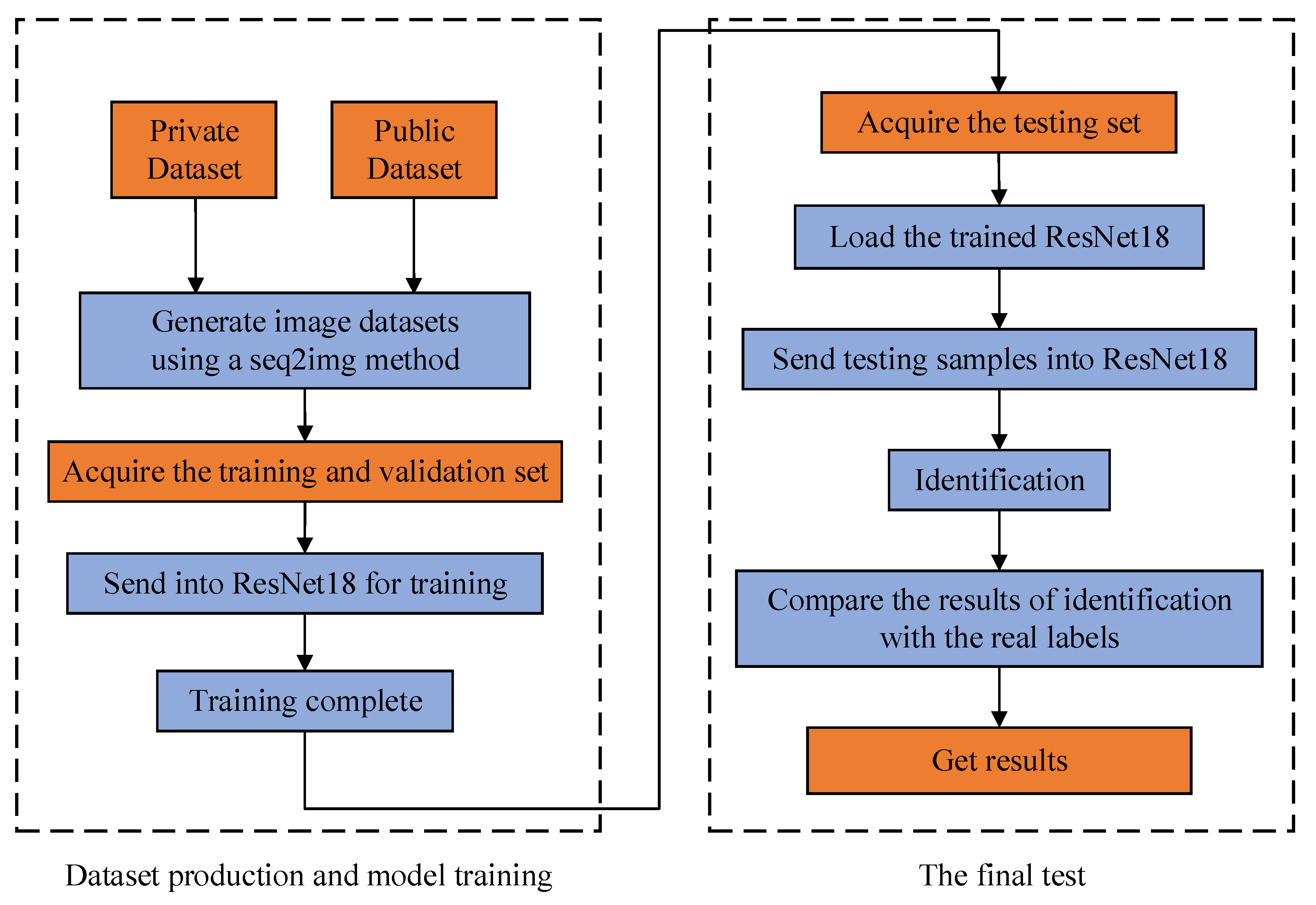
In this paper, several experiments are constructed based on the selection of datasets and seq2img methods. The overall process of the experiment is shown in Figure 10, and the arrangement of the experiment is as follows.

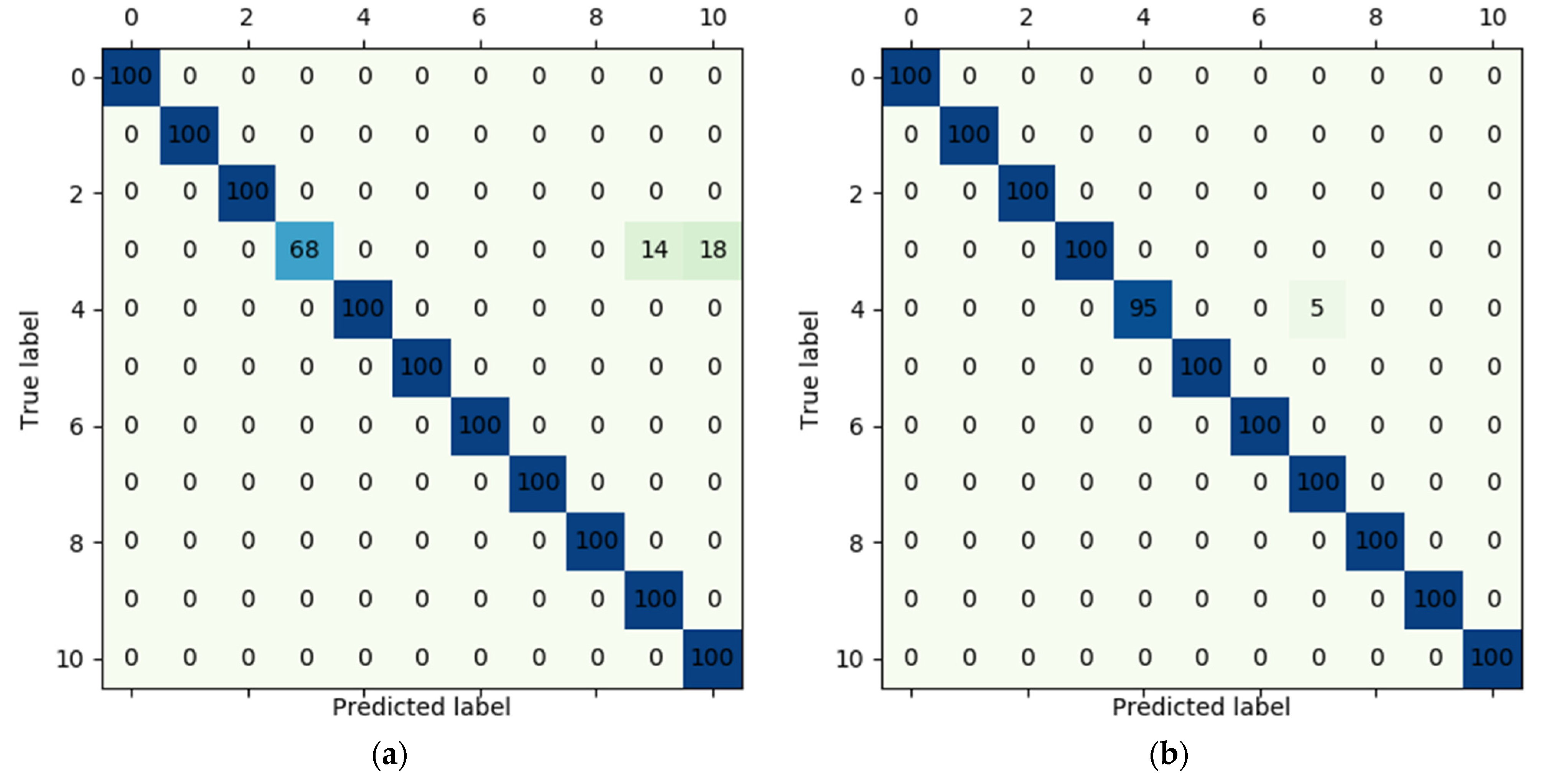
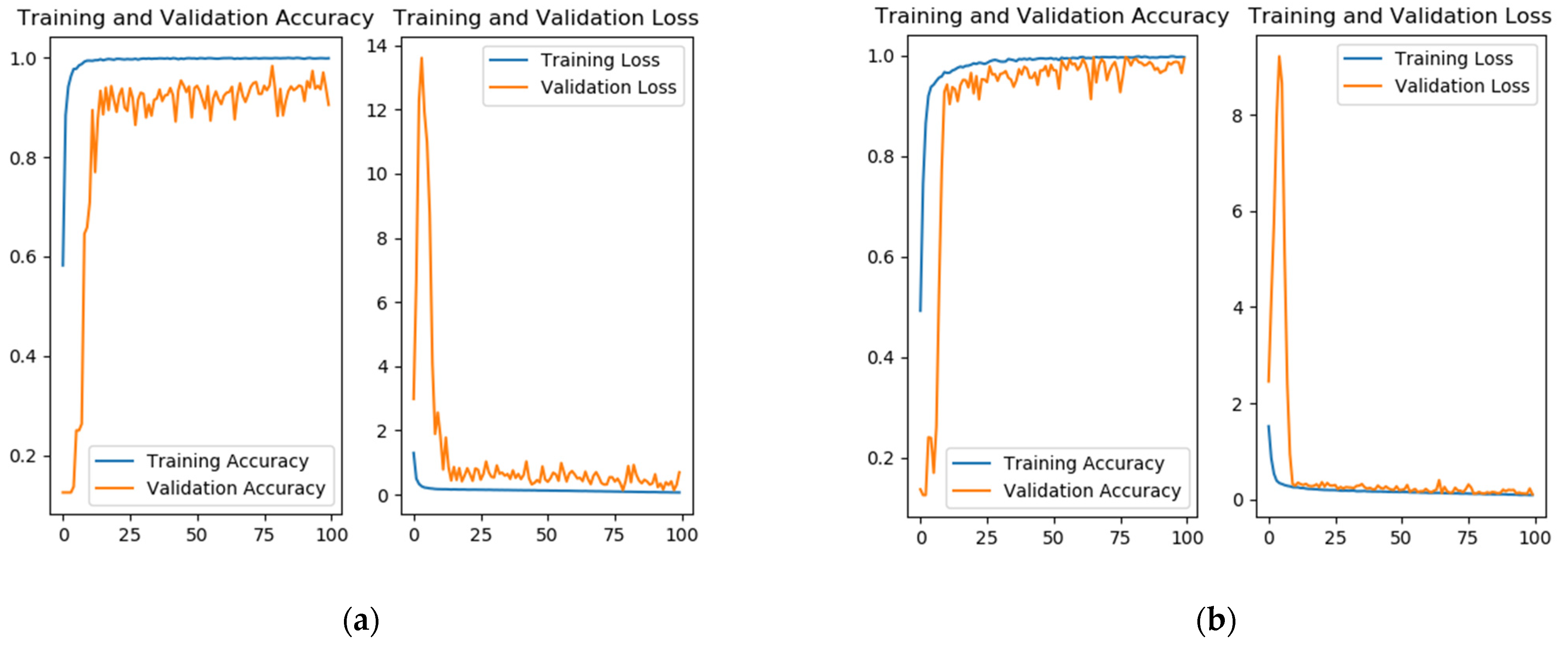
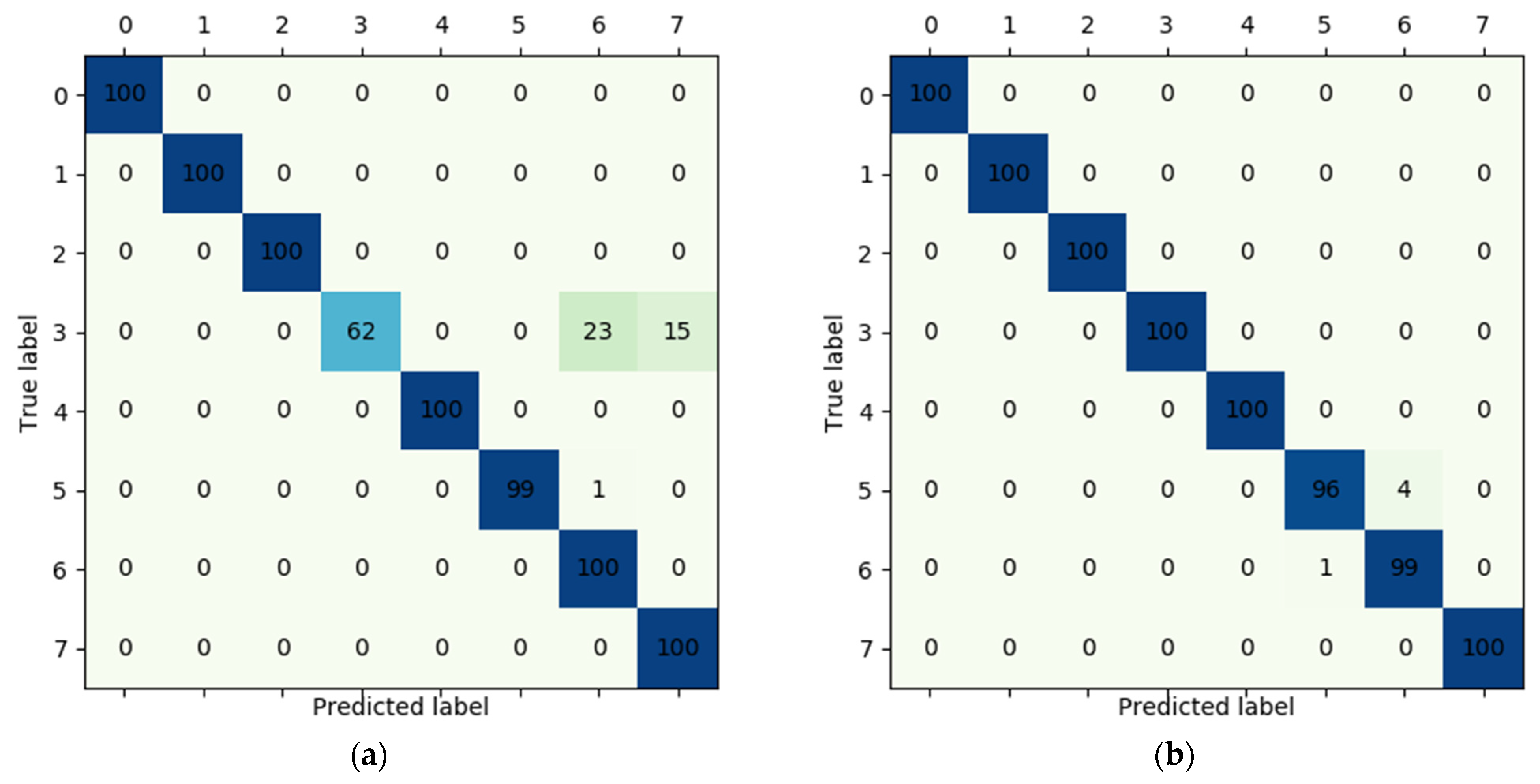
In the first experiment, the ESEAD dataset is coded using the general GAF and iGAF to generate the GAF-ESEAD image dataset and iGAF-ESEAD image dataset, which are then used for the ResNet18 training to obtain the GAF-ResNet-S model and the iGAF-ResNet-S model. Finally, the test set in the ESEAD dataset is applied to the GAF-ResNet-S model and iGAF-ResNet-S model for performance comparisons. Here, various evaluation metrics are used, including precision, recall, and F1 score.

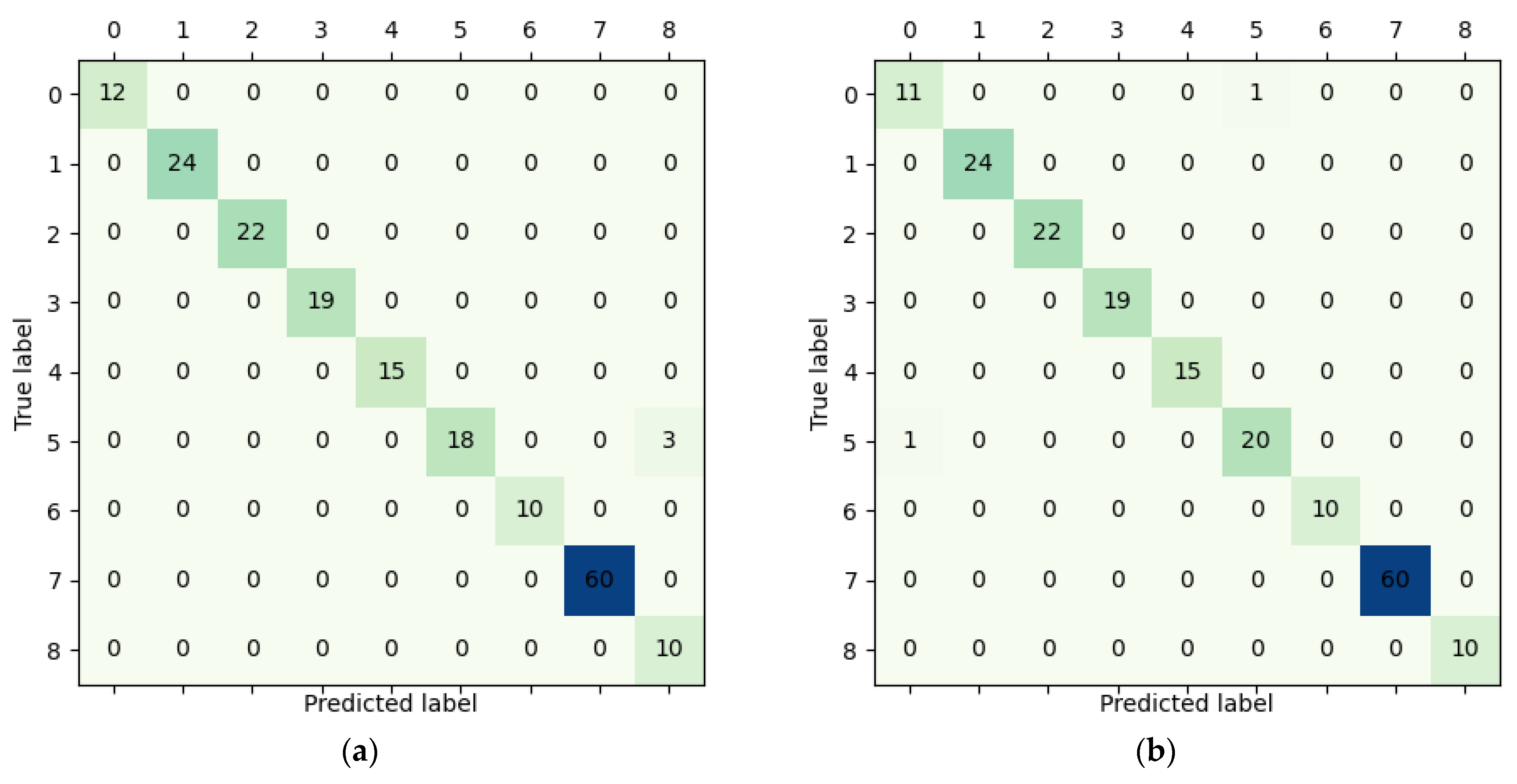
In the second experiment, the same experimental procedure is performed on the EMCAD dataset. Precision, recall, and F1 score are used to evaluate the experimental results.

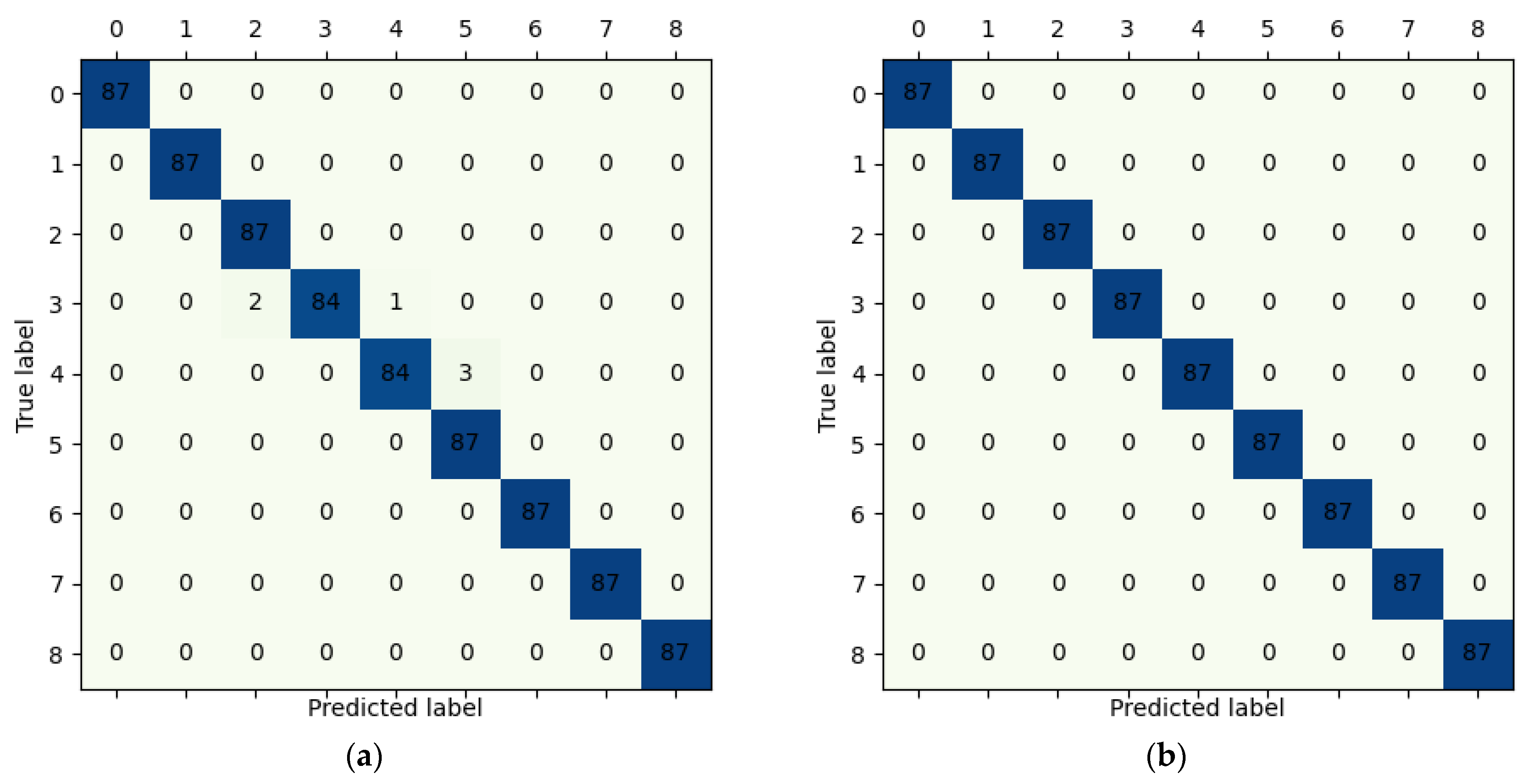
In the third experiment, the experimental PLAID and experimental WHITED datasets are used to validate the proposed method. GAF images and iGAF images are generated based on these two public datasets to train the ResNet18. The overall identification accuracy (OIA) is the evaluation metric for evaluating the performance of the model.

Furthermore, in the fourth experiment, for comparing the proposed method with other NILM methods based on seq2img, another four seq2img methods, V-I trajectory, color V-I trajectory, MTF, and RG, are used to code the ESEAD, EMCAD, PLAID, and WHITED dataset. The overall identification accuracy is adopted to evaluate the identification performance.

The hyperparameters of the models are constant. Each generated image has a resolution of 100 by 100 pixels and contains a total of 10,000 pixels. It should be noted that the fact that each image contains 10,000 pixels does not mean that the image contains data of 10,000 sampling points. Each image is converted from its corresponding sample through a seq2img method, so the information contained in each image is the information of a sample containing 1000 sampling points. The adaptive moment estimation (Adam) is used as the parameter optimizer with a learning rate of 0.00001, a first-order decay rate of 0.9, and a second-order decay rate of 0.999. 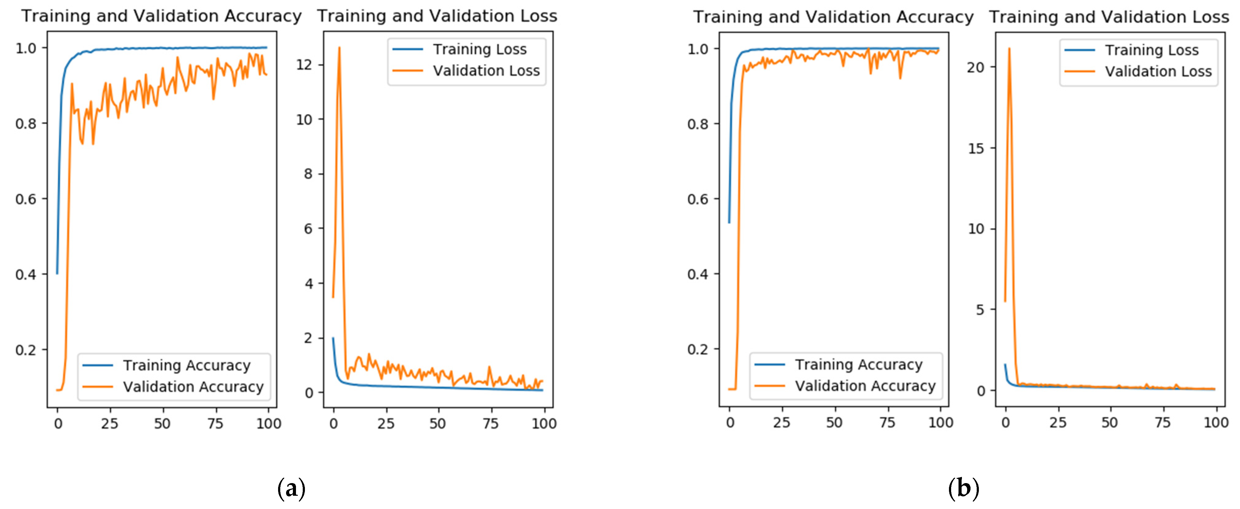Adam is straightforward to implement and computationally efficient [32]. The batch size is set at 80 to balance the data operation of the model with fast convergence without exceeding the GPU memory. To prevent underfitting and overfitting, the training process will run 100 epochs. The loss function is sparse categorical cross-entropy.

All models are deployed on a computer with an Intel Core i7-8750H hexacore CPU and NVIDIA GeForce GTX 1060 GPU. An open-source framework TensorFlow 2.1.0, the deep learning platform based on Python 3.7, is used for program implementation.

4.4. Evaluation Metrics

Here, three parameters, precision (PR), recall (RCL), and $F_{\beta }$ score (FS) are defined to evaluate the load identification performance [33]. The calculations are as follows:

$$P{R}_j=\frac{T{P}_j}{T{P}_j+F{P}_j}$$

(14)

$$RC{L}_j=\frac{T{P}_j}{T{P}_j+F{N}_j}$$

(15)

$$F{S}_j=\left(1+{\beta }^2\right)\cdot \frac{P{R}_j\cdot RC{L}_j}{{\beta }^2\cdot P{R}_j+RC{L}_j}$$

(16)

where $T{P}_j$ is the true positive, i.e., the number of samples when the predicted category is j, and the actual category is j; $F{P}_j$ is the false positive, i.e., the number of samples when the predicted category is j, and the actual category is not $j$; $F{N}_j$ is the false negative, i.e., the number of samples when the predicted category is not $j$, and the actual category is $j$. $\beta ={\omega }_{RCL}/{\omega }_{PR}$ is the weighting ratio of RCL to PR. Since RC and PR are both important indicators, $\beta =1$ is used.

Moreover, the overall identification accuracy ($OIA$), which is defined in (17), will be used to evaluate the overall performance of the model.

$$OIA=\frac{CI}{I}$$

(17)

where $CI$ is the number of correct identifications; $I$ is the total number of identifications.

5. Results and Discussion

5.1. Comparison with the Method Based on the General GAF

5.1.1. Discussion of the Results for Experiments on the ESEAD Dataset

In this section, experiments are conducted based on the ESEAD dataset. There are 11,000 samples, including 7700 training samples, 2200 validation samples, and 1100 test samples. Results of the GAF-ResNet-S model and the iGAF-ResNet-S model are shown in

Table 6. Results for the experiments of single categories.

Label	Category	The General Method			The Proposed Load Identification Method
		PR	RCL	FS	PR	RCL	FS
0	Induction Cooker (standby)	1	1	1	1	1	1
1	Induction Cooker (running)	1	1	1	1	1	1
2	Desktop	1	1	1	1	1	1
3	Tablet	1	0.68	0.809	1	1	1
4	Printer	1	1	1	1	0.95	0.974
5	Coffee Machine	1	1	1	1	1	1
6	Microwave Oven (running)	1	1	1	1	1	1
7	Microwave Oven (standby)	1	1	1	0.952	1	0.975
8	Electric soldering iron	1	1	1	1	1	1
9	Laptop	0.877	1	0.934	1	1	1
10	Smartphone	0.847	1	0.917	1	1	1

. The curves of the classification accuracy changing with the number of iterations in the training process are shown in Figure 11. It can be seen that the convergence of the iGAF-ResNet-S model is faster, the identification performance after convergence is more stable, and the loss is lower.

It can be seen from Table 6 that for the method based on the general GAF, the recall of category 3 is low, which also leads to the low value of the F1 score. Similar results can be found in category 9 and category 10. Both the precision and F1 score are smaller than those of improved identifications. Due to these low values, it is seen from the confusion matrix shown in Figure 12a that there are 32 samples out of 100 of category 3 being falsely identified as category 9 and 10.

From the confusion matrix shown in Figure 12b, we can see that by using the method based on the iGAF, the identification accuracy of the improved method for categories 3, 9, and 10 has been improved to 100%. It is noted that there is around a 5% error for category 4 of the improved method, which caused a small drop in the F1 scores of category 4 and category 7. Even though it is seen that the overall identification accuracy is improved from 97.09% to 99.55% by using the proposed method.

5.1.2. Discussion of the Results for Experiments on the EMCAD Dataset

In this section, experiments are conducted based on the EMCAD dataset. There are 8000 samples in this dataset, including 5600 training samples, 1600 validation samples, and 800 test samples. The results of the three evaluation parameters are illustrated in

Table 7. Results for the experiments of mixed categories.

Label	Category	The General Method			The Proposed Load Identification Method
		PR	RCL	FS	PR	RCL	FS
0	Induction Cooker + Microwave Oven	1	1	1	1	1	1
1	Induction Cooker	1	1	1	1	1	1
2	Desktop	1	1	1	1	1	1
3	Tablet	1	0.62	0.765	1	1	1
4	Microwave Oven + Smartphone	1	1	1	1	1	1
5	Tablet + Desktop	1	0.99	0.995	0.989	0.96	0.974
6	Smartphone + Laptop	0.813	1	0.897	0.961	0.99	0.975
7	Smartphone	0.869	1	0.929	1	1	1

. The curves of the classification accuracy changing with the number of iterations in the training process are shown in Figure 13. It can be seen that the convergence of the iGAF-ResNet-M model is faster, the identification performance after convergence is more stable, and the loss is lower.

The confusion matrices of the general method and the improved method are shown in Figure 14. It can be seen from Figure 14a that when the model training is performed with the images generated by the general GAF, category 3 (tablet) is incorrectly identified as category 6 (smartphone + laptop) 23 times and is incorrectly identified as category 7 (smartphone) 15 times. This results in lower recall and F1 scores for category 3, which are 0.62 and 0.765, respectively, as shown in Table 5. At the same time, the precision and F1 scores of category 6 and category 7 are getting decreased because of the confusion between category 3, category 6, and category 7.

By using the proposed method, as shown in Table 7, the recall of category 3 is improved from 0.62 to 1, and the F1 score is increased from 0.765 to 1. The precision of category 6 is improved from 0.813 to 0.961, and the precision of category 7 reaches 1. The F1 score of category 7 and category 8 are improved to 0.975 and 1, respectively. Meanwhile, it can be seen from Figure 14b that confusion between category 3, category 6, and category 7 is eliminated. The overall accuracy of the improved load identification reaches 99.375%, which is 4.25% more than the general method.

5.1.3. Discussion of the Results for Experiments on Public Datasets

In this section, experiments are conducted based on the experimental PLAID and experimental WHITED datasets. There are 1910 samples in the experimental PLAID dataset, including 1336 training samples, 381 validation samples, and 193 test samples. The confusion matrices of the general method and the improved method are shown in Figure 15. In the experimental WHITED dataset, there are 7830 samples, including 5481 training samples, 1566 validation samples, and 783 test samples. The confusion matrices of the general method and the improved method are shown in Figure 16. Since the confusion between loads is not significant in both datasets, we only use the OIA as the evaluation metric for assessing the model performance. The results are shown in

Table 8. The overall identification accuracy on PLAID and WHITED.

Public Dataset	The Trained Model	OIA
PLAID	GAF-ResNet model	98.446%
PLAID	iGAF-ResNet model	98.964%
WHITED	GAF-ResNet model	99.234%
WHITED	iGAF-ResNet model	100%

.

As can be seen from Figure 15 and Figure 16, benefiting from the feature expression power of GAF and iGAF and the high-quality data collection of the public datasets, the confusion of loads does not occur significantly in both datasets. From Table 8, we can see that although both GAF-based and iGAF-based models achieve high OIA, the ResNet18 trained with iGAF images demonstrates further improvement compared to the ResNet18 trained with general GAF images under the same training conditions. It even achieved 100% accuracy on the WHITED dataset. This indicates that even in datasets without easily confused loads, the proposed method demonstrates better identification performance compared to the general method.

On the other hand, through a comprehensive comparison of the performance of the general method and the proposed method on the ESEAD, EMCAD, PLAID, and WHITED datasets, it can be observed that methods achieving high identification accuracy on public datasets may still encounter challenges when applied to specific scenarios. General methods exhibit good performance on public datasets but fail to effectively address the load confusion problem in the ESEAD and EMCAD datasets, which are based on different application scenarios. However, the proposed method performs well on both public datasets and the ESEAD and EMCAD datasets, indicating its capability to handle general scenarios in public datasets and effectively address the specific scenarios in the ESEAD and EMCAD datasets.

5.2. Comparison with Other NILM Methods

In

Table 9. Related works about NILM methods.

Related Work	Seq2img Method	Model	Dataset
Davies et al. [6]	/	VGGNet	PLAID
Baets et al. [8]	V-I trajectory	CNN	PLAID
Liu et al. [10]	Color V-I trajectory	AlexNet	PLAID, WHITED
Wenninger et al. [14]	RG	SPPCNN	COOLL, PLAID, WHITED
Faustine et al. [12]	RG	CNN	LILACD, PLAID
Wang et al. [15]	GAF, MTF	CNN, DA	ECG, CBF, Gun Point et al.
Proposed Method	iGAF	ResNet18	PLAID, WHITED, Private

, several NILM methods are presented. It can be observed that due to various differences in experimental settings and validation procedures among these works, it becomes challenging to make a fair comparison between the proposed NILM method and the other NILM methods [34]. For instance, the results in [6] are not derived from the seq2img-based NILM method. Experiments in [15] cover a considerable number of datasets, but commonly used public datasets, such as the PLAID dataset, are not included. All the related works have not been tested on private datasets, thus making it unreasonable to compare them with our experimental results on the ESEAD and EMCAD datasets. Additionally, different deep-learning frameworks are used in these works. Most of them are based on CNN, but the network structures are fine-tuned according to their respective datasets during the experimental processes. Therefore, the experimental results in these works cannot be directly compared to the experimental results presented in this paper.

Considering the aforementioned factors, we adopted a compromise experimental approach, which involves replacing the seq2img method proposed in this paper with the seq2img method used in other related works while keeping the experimental settings consistent with those described in this paper. We conducted experiments on the ESEAD, EMCAD, PLAID, and WHITED datasets, following the same experimental procedures as described in this paper. Since the advantage of the proposed method lies in its superior seq2img method, conducting experiments with the same experimental settings but different seq2img methods will better validate the feasibility of the proposed method.

5.2.1. Discussion of the Results for Experiments on the ESEAD and EMCAD

In this section, V-I trajectory, color V-I trajectory, MTF, and RG are used to code the raw data in the ESEAD and EMCAD datasets. Based on the ESEAD dataset, VI-ESEAD image, color VI-ESEAD image, MTF-ESEAD image, and RG-ESEAD image datasets are generated. Based on the EMCAD dataset, VI-EMCAD image, color VI-EMCAD image, MTF-EMCAD image, and RG-EMCAD image datasets are generated. By training ResNet18 using the aforementioned eight image datasets, eight models can be obtained. After inputting the test data, the OIA of all models is shown in

Table 10. The overall identification accuracy of different methods on ESEAD and EMCAD datasets.

ESEAD Dataset		EMCAD Dataset
Seq2img Method	OIA of Trained Model	Seq2img Method	OIA of Trained Model
V-I trajectory	73.272%	V-I trajectory	75.375%
Color V-I trajectory	91.363%	Color V-I trajectory	89.625%
MTF	94.818%	MTF	99.625%
RG	76.272%	RG	92.500%
iGAF	99.545%	iGAF	99.375%

, and the OIA of the iGAF-based method is also listed in the table for comparison.

As can be seen in Table 8, using V-I trajectory as the seq2img method, the trained model achieves quite low OIA with only 73.272% and 75.375% on the two datasets, respectively. In contrast, the model trained with color V-I trajectory as the seq2img method shows a significant improvement in OIA, indicating that incorporating color information is beneficial for enhancing the identification performance of the model. The MTF method reaches an OIA exceeding 90% on both datasets, slightly surpassing iGAF in the EMCAD dataset. The RG method achieves an OIA of over 90% on the EMCAD dataset but performs poorly on the ESEAD dataset. The iGAF method surpasses 99% OIA on both the ESEAD and EMCAD datasets, indicating that the images generated by the iGAF method possess superior feature representation capabilities compared to images generated by other seq2img methods.

5.2.2. Discussion of the Results for Experiments on PLAID and WHITED

In this section, V-I trajectory, color V-I trajectory, MTF, and RG are used to code the raw data in PLAID and WHITED datasets. Based on the PLAID dataset, VI-PLAID image, color VI-PLAID image, MTF-PLAID image, and RG-PLAID image datasets are generated. Based on the WHITED dataset, VI-WHITED image, color VI-WHITED image, MTF-WHITED image, and RG-WHITED image datasets are generated. Training ResNet18 using the above eight image datasets and inputting the test data, the overall identification accuracy of trained models is shown in

Table 11. The overall identification accuracy of different methods on PLAID and WHITED datasets.

PLAID Dataset		WHITED Dataset
Seq2img Method	OIA of Trained Model	Seq2img Method	OIA of Trained Model
V-I trajectory	78.756%	V-I trajectory	74.074%
Color V-I trajectory	94.818%	Color V-I trajectory	96.041%
MTF	97.409%	MTF	69.859%
RG	93.782%	RG	76.884%
iGAF	98.964%	iGAF	100%

.

It is evident from Table 11 that models trained with iGAF as the seq2img method have higher OIA. The color V-I trajectory performs remarkably well on both datasets, obtaining over 90% accuracy, while the model trained using V-I trajectory as the seq2img method still has the lowest amount of OIA. The MTF and RG methods perform well on the PLAID dataset but show poor performance on the WHITED dataset. On the other hand, iGAF demonstrates high OIA on both datasets, with a noteworthy OIA of 100% on the WHITED dataset. This indicates that the iGAF method performs better than other seq2img methods on public datasets.

Based on the above discussion, the models trained with iGAF as the seq2img method exhibit the highest overall identification accuracy compared to other methods on both public and private datasets. Under the same experimental conditions and procedures, the images generated by the iGAF method possess superior feature representation capabilities compared to images generated by other seq2img methods. The nonintrusive load identification method based on iGAF and ResNet18 demonstrates superior identification performance than other NILM methods.

6. Conclusions

In this article, an improved method of GAF is studied, and a nonintrusive load identification method based on the improved GAF and ResNet18 is proposed. The amplitude Gramian matrix and phase Gramian matrix are calculated based on the fast Fourier transform and the calculation of the Gramian matrix. It is found that by assigning the values of the raw data Gramian matrix, the amplitude Gramian matrix, and the phase Gramian matrix to the pixel matrices of the B channel, G channel, and R channel, the amplitude and phase features of the raw data can be added to the generated images. Hence, the recognizability loads with similar current signals are improved. Experiments are performed based on two private datasets and two public datasets. Results show that, with the improved load identification method, the overall identification accuracies on four datasets are improved, and the identification accuracies of easily confused loads in the two private datasets are significantly increased.

In future research, the lightweight and deployment of the algorithm should be considered. The number of parameters to be trained in the algorithm should be further reduced, and the computing efficiency on edge computing devices with low computing power should be further improved.

References

1. Hart, G.W. Nonintrusive appliance load monitoring. Proc. IEEE 1992, 80, 1870–1891. [Google Scholar] [CrossRef]
2. Kolter, J.Z.; Jaakkola, T. Approximate inference in additive factorial hmms with application to energy disaggregation. In Proceedings of the Fifteenth International Conference on Artificial Intelligence and Statistics, La Palma, Canary Islands, Spain, 21–23 April 2012. [Google Scholar]
3. Taveira, P.R.Z.; Moraes, C.D.; Lambert-Torres, G. Non-intrusive identification of loads by random forest and fireworks optimization. IEEE Access 2020, 8, 75060–75072. [Google Scholar] [CrossRef]
4. Lam, H.Y.; Fung, G.S.K.; Lee, W.K. A novel method to construct taxonomy electrical appliances based on load signa-turesof. IEEE Trans. Consum. Electron. 2007, 53, 653–660. [Google Scholar] [CrossRef] [Green Version]
5. Kelly, J.; Knottenbelt, W. Neural NILM: Deep neural networks applied to energy disaggregation. In Proceedings of the 2nd ACM International Conference on Embedded Systems for Energy-Efficient Built Environments, Seoul, Republic of Korea, 4–5 November 2015; pp. 55–64. [Google Scholar]
6. Davies, P.; Dennis, J.; Hansom, J.; Martin, W.; Stankevicius, A.; Ward, L. Deep neural networks for appliance transient classification. In Proceedings of the ICASSP 2019—2019 IEEE International Conference on Acoustics, Speech and Signal Processing (ICASSP), Brighton, UK, 12–17 May 2019; pp. 8320–8324. [Google Scholar]
7. Xu, X.H.; Zhao, S.T.; Cui, K.B. Non-intrusive load decomposition algorithm based on convolutional block attention module. Power Syst. Technol. 2021, 45, 3700–3706. [Google Scholar]
8. Baets, L.D.; Ruyssinck, J.; Develder, C.; Dhaene, T.; Deschrijver, D. Appliance classification using VI trajectories and convolutional neural networks. Energy Build. 2018, 158, 32–36. [Google Scholar] [CrossRef] [Green Version]
9. Gao, J.K.; Kara, E.C.; Giri, S.; Bergés, M. A feasibility study of automated plug-load identification from high-frequency measurements. In Proceedings of the 2015 IEEE Global Conference on Signal and Information Processing (GlobalSIP) 2015, Orlando, FL, USA, 14–16 December 2015; pp. 220–224. [Google Scholar]
10. Liu, Y.C.; Wang, X.; You, W. Non-intrusive load monitoring by voltage–current trajectory enabled transfer learning. IEEE Trans. Smart Grid 2019, 10, 5609–5619. [Google Scholar] [CrossRef]
11. Faustine, A.; Pereira, L. Improved appliance classification in non-intrusive load monitoring using weighted recurrence graph and convolutional neural networks. Energies 2020, 13, 3374. [Google Scholar] [CrossRef]
12. Faustine, A.; Pereira, L.; Klemenjak, C. Adaptive weighted recurrence graphs for appliance recognition in non-intrusive load monitoring. IEEE Trans. Smart Grid 2020, 12, 398–406. [Google Scholar] [CrossRef]
13. Wenninger, M.; Bayerl, S.P.; Schmidt, J.; Riedhammer, K. Timage—A robust time series classification pipeline. In Proceedings of the ICANN19, 28th International Conference on Artificial Neural Networks, Munich, Germany, 17–19 September 2019. [Google Scholar]
14. Wenninger, M.; Bayerl, S.P.; Maier, A.; Schmidt, J. Recurrence plot spacial pyramid pooling network for appliance identification in non-intrusive load monitoring. In Proceedings of the 2021 20th IEEE International Conference on Machine Learning and Applications (ICMLA), Pasadena, CA, USA, 13–16 December 2021. [Google Scholar]
15. Wang, Z.G.; Oates, T. Imaging time-series to improve classification and imputation. In Proceedings of the 24th International Conference on Artificial Intelligence, Buenos Aires, Argentina, 25 July 2015; pp. 3939–3945. [Google Scholar]
16. Gao, A.; Zheng, J.Y.; Mei, F.; Sha, H.Y.; Qiu, X.; Xie, Y.; Li, X.; Guo, M.L.; Li, D.Q. Electricity theft detection algorithm based on triplet network. Proc. Chin. Soc. Electr. Eng. 2022, 42, 3975–3986. [Google Scholar]
17. Li, K.X.; Yin, B.; Du, Z.H.; Sun, Y.F. A nonintrusive load identification model based on time-frequency features fusion. IEEE Access 2021, 9, 1376–1387. [Google Scholar] [CrossRef]
18. Qu, L.T.; Kong, Y.G.; Li, M.; Dong, W.; Zhang, F.; Zuo, H.B. A residual convolutional neural network with multi-block for appliance recognition in non-intrusive load identification. Energy Build. 2023, 281, 112749. [Google Scholar] [CrossRef]
19. Chen, J.F.; Wang, X. Non-intrusive Load Monitoring Using Gramian Angular Field Color Encoding in Edge Computing. Chin. J. Electron. 2022, 31, 595–603. [Google Scholar] [CrossRef]
20. Zhang, Y.S.; Wu, H.; Ma, Q.; Yang, Q.R.; Wang, Y.W. A Learnable Image-Based Load Signature Construction Approach in NILM for Appliances Identification. IEEE Trans. Smart Grid 2023. early access. [Google Scholar] [CrossRef]
21. Kim, H.; Lim, S. Temporal Patternization of Power Signatures for Appliance Classification in NILM. Energies 2021, 14, 2931. [Google Scholar] [CrossRef]
22. Duhamel, P.; Vetterli, M. Fast Fourier transforms: A tutorial review and a state of the art. Signal Process. 1990, 19, 259–299. [Google Scholar] [CrossRef] [Green Version]
23. Brigham, E.O.; Morrow, R.E. The fast Fourier transform. IEEE Spectr. 1967, 4, 63–70. [Google Scholar] [CrossRef]
24. Hu, X.M.; Peng, Y.G.; Mo, H.J.; Cai, T.T.; Deng, Q.T. An improved time–frequency feature fusion based nonintrusive load monitor for load identification. In Proceedings of the 2022 2nd International Conference on Electrical Engineering and Mechatronics Technology (ICEEMT), Hangzhou, China, 1–3 July 2022. [Google Scholar]
25. Hong, Y.Y.; Martinez, J.J.F.; Fajardo, A.C. Day-Ahead Solar Irradiation Forecasting Utilizing Gramian Angular Field and Convolutional Long Short-Term Memory. IEEE Access 2020, 8, 18741–18753. [Google Scholar] [CrossRef]
26. Keogh, E.J.; Pazzani, M.J. Scaling up dynamic time warping for datamining applications. In Proceedings of the Sixth ACM SIGKDD International Conference on Knowledge Discovery and Data Mining, Boston, MA, USA, 20–23 August 2000; pp. 285–289. [Google Scholar]
27. He, K.M.; Zhang, X.Y.; Ren, S.Q.; Sun, J. Deep residual learning for image recognition. In Proceedings of the 2016 IEEE Conference on Computer Vision and Pattern Recognition (CVPR), Las Vegas, NV, USA, 27–30 June 2016; pp. 770–778. [Google Scholar]
28. Seidaliyeva, U.; Alduraibi, M.; Ilipbayeva, L.; Smailov, N. Deep residual neural network-based classification of loaded and unloaded UAV images. In Proceedings of the 2020 Fourth IEEE International Conference on Robotic Computing (IRC), Taichung, Taiwan, 9–11 November 2020; pp. 465–469. [Google Scholar]
29. Lesnikov, V.; Naumovich, T.; Chastikov, A. Aliasing’s Study on Bandpass Sampling. In Proceedings of the 2022 Systems of Signal Synchronization, Generating and Processing in Telecommunications (SYNCHROINFO), Arkhangelsk, Russia, 29 June–1 July 2022; pp. 1–6. [Google Scholar]
30. Gao, J.K.; Giri, S.; Kara, E.C.; Bergés, M. PLAID: A public dataset of high-resoultion electrical appliance measurements for load identification research. In Proceedings of the 1st ACM Conference on Embedded Systems for Energy-Efficient Buildings, Memphis, TN, USA, 3–6 November; pp. 198–199.
31. Kahl, M.; Haq, A.U.; Kriechbaumer, T.; Jacobsen, H.A. WHITED—A Worldwide Household and Industry Transient Energy Data Set. In Proceedings of the 3rd International Workshop on Non-Intrusive Load Monitoring, Simon Fraser University, Vancouver, BC, Canada, 14–15 May 2016. [Google Scholar]
32. Kingma, D.P.; Ba, J. Adam: A Method for Stochastic Optimization. In Proceedings of the 3rd International Conference for Learning Representations, San Diego, CA, USA, 7–9 May 2015. [Google Scholar]
33. Mahmud, A.A. Artificial Intelligence (AI)-based identification of appliances in households through NILM. In Proceedings of the 2022 4th Global Power, Energy and Communication Conference (GPECOM), Nevsehir, Turkey, 14–17 June 2022; pp. 414–426. [Google Scholar]
34. Faustine, A.; Pereira, L. Multi-Label Learning for Appliance Recognition in NILM Using Fryze-Current Decomposition and Convolutional Neural Network. Energies 2020, 13, 4154. [Google Scholar] [CrossRef]
Figure 1. The flow chart of improved Gramian angular field.
Electronics 12 02540 g001
Figure 2. (a) GAF images of tablet, laptop, and smartphone; (b) iGAF images of tablet, laptop, and smartphone.
Electronics 12 02540 g002
Figure 3. The principle of the three-channel convolution kernel.
Electronics 12 02540 g003
Figure 4. The residual block.
Electronics 12 02540 g004
Figure 5. Workflow of the proposed load identification method based on the iGAF and ResNet18.
Electronics 12 02540 g005
Figure 6. Equipment for data collection and the diagram of connection.
Electronics 12 02540 g006
Figure 7. Current waveforms of eleven different appliances: (a) induction cooker (standby); (b) induction cooker (running); (c) desktop; (d) tablet; (e) printer; (f) coffee machine; (g) microwave oven (standby); (h) microwave oven (running); (i) electric soldering iron; (j) laptop; (k) smartphone.
Electronics 12 02540 g007
Figure 8. Current waveforms of eight different appliance combinations: (a) induction cooker + tablet; (b) induction cooker + microwave oven; (c) induction cooker + smartphone; (d) microwave oven + tablet; (e) microwave + smartphone; (f) tablet + desktop; (g) tablet + smartphone; (h) smartphone + laptop.
Electronics 12 02540 g008
Figure 9. Split of samples.
Electronics 12 02540 g009
Figure 10. The overall process of the experiment.
Electronics 12 02540 g010
Figure 11. Model accuracy and loss graphs: (a) GAF-ResNet-S model; (b) iGAF-ResNet-S model.
Electronics 12 02540 g011
Figure 12. Confusion matrices: (a) GAF-ResNet-S method; (b) iGAF-ResNet-S method.
Electronics 12 02540 g012
Figure 13. Model accuracy and loss graphs: (a) GAF-ResNet-M model; (b) iGAF-ResNet-M model.
Electronics 12 02540 g013
Figure 14. Confusion matrices: (a) GAF-ResNet-M method; (b) iGAF-ResNet-M method.
Electronics 12 02540 g014
Figure 15. Confusion matrices: (a) general method on PLAID; (b) proposed method on PLAID.
Electronics 12 02540 g015
Figure 16. Confusion matrices: (a) general method on WHITED; (b) proposed method on WHITED.
Electronics 12 02540 g016