Study on Body Size Measurement Method of Goat and Cattle under Different Background Based on Deep Learning

Abstract

The feasibility of using depth sensors to measure the body size of livestock has been extensively tested. Most existing methods are only capable of measuring the body size of specific livestock in a specific background. In this study, we proposed a unique method of livestock body size measurement using deep learning. By training the data of cattle and goat with same feature points, different animal sizes can be measured under different backgrounds. First, a novel penalty function and an autoregressive model were introduced to reconstruct the depth image with super-resolution, and the effect of distance and illumination on the depth image was reduced. Second, under the U-Net neural network, the characteristics exhibited by the attention module and the DropBlock were adopted to improve the robustness of the background and trunk segmentation. Lastly, this study initially exploited the idea of human joint point location to accurately locate the livestock body feature points, and the livestock was accurately measured. According to the results, the average accuracy of this method was 93.59%. The correct key points for detecting the points of withers, shoulder points, shallowest part of the chest, highest point of the hip bones and ischia tuberosity had the percentages of 96.7%, 89.3%, 95.6%, 90.5% and 94.5%, respectively. In addition, the mean relative errors of withers height, hip height, body length and chest depth were only 1.86%, 2.07%, 2.42% and 2.72%, respectively.

1. Introduction

As precision animal husbandry is leaping forward, scientific feeding and management can help producers gain insights into the health and overall welfare of livestock. Accordingly, body measurement turns out to be a vital indicator to assess fat deposition and energy metabolism of livestock [1]. Conventional measurement methods mainly exploit tools for the measurement. Besides the time-consuming characteristic and high costs, livestock will come into contact with measurement processes. The stress response of livestock affects measurement accuracy while causing personal injury [2]; therefore, it is necessary to develop an automated measurement method instead of manual measurement.

Against the defects of conventional methods, computer vision has been adopted in livestock body size measurement [3]. The feasibility of using 2D images has been proven to measure the body size of goat [4,5], pig [6,7], cattle [8,9], horses [10], and other livestock; however, measurements by 2D images without depth information were often inaccurate [11,12]. With the emergence of depth sensors (e.g., Kinect, Intel Realsense and ASUS-Xtion), 3D images with depth information have been used for more accurate body size measurement of livestock.

For pigs, Wang et al. [13] and Shi et al. [14] used random sample consensus to remove the background point cloud, and the body measurements were acquired by calculating the integral length of the curve. For cattle, Salau et al. [12] manually marked the feature points and calculated the cattle body size with the Cartesian coordinates. The feature point marking method was then optimized by Ruchay et al. [15]; the filters were used to remove the noises in the depth map and marked feature points in cattle. For goats, Lina et al. [16] detected the feature points by finding the convex to calculate the goat’s body size. Guo et al. [17,18] developed the LSSA_CAU system to measure the body sizes of pigs, horses and cattle in their respective scenes, exploiting the unevenness of the first derivative of the point cloud curve to find the feature points of livestock; however, all the above research on livestock body size measurement analyzed a single livestock species in a specific scene, and the measurement accuracy was greatly influenced by illumination, background and livestock species, and therefore it does not have wide application value.

To obtain a widely applicable method based on existing studies, the related research in livestock body size measurement should focus on how to overcome the influence of illumination, background and livestock species to obtain high-quality point clouds and accurate feature points. Numerous researchers have completed background segmentation and body-part segmentation of livestock by deep learning [5,19,20,21,22]; however, this research has also been limited to single livestock species and has poor robustness to livestock species and background noise. Further research is needed for multi-species segmentation by deep learning. For feature point location, feature point could be located by image segmentation [9,23,24] and statistical learning [14,25]. The accuracy of image segmentation and statistical learning is determined by feature engineering construction. Compared to manual feature engineering construction, deep learning is capable of extracting better feature expressions. Currently, the research on using deep learning to locate the feature points in livestock is rare.

As revealed from the mentioned research, various livestock exhibit unique morphological characteristics; however, most methods only apply to the body size measurement of one species of livestock, and they are affected by background, illuminations and livestock species. Though deep learning technology has made great progress, it needs further study in the livestock body size measurement; thus, this study developed a measurement method of body size for different livestock species based on deep learning. For adult livestock with the same body size feature points, the deep learning technology was used to complete the livestock background segmentation, the trunk segmentation and the feature point location. This study could be referenced for using the deep learning technology to measure the body size of livestock.

The rest of this study is organized as follows. In the Section 2, the materials and methods are described. In the Section 3, the experimental results are presented and discussed. In the Section 4, the conclusion of this study and subsequent studies are summarized.

2. Materials and Methods

2.1. Data Set

2.1.1. Data Acquisition

In this study, used the Intel RealSense D415 depth camera (Intel™, Santa Clara, CA, USA) with both handheld and fixed shooting to collect video data of 30 adult cattle (Simmental cattle and Holstein Friesian, age > 36 months) and 25 adult goats (Chengde hornless goat, age > 24 months) in April and November. Animal videos were collected in different illumination, different distances and different angle under the scope of the camera’s depth horizontal field of view (±69.4°), color horizontal field of view (±69.4°) and the acquisition range of the depth camera (16–200 cm). The camera’s field of view was ensured to cover the feature points of the livestock. The average video duration of the respective livestock was 120 s. The resolution of color video and depth video reached 1280 × 720 pixels, and the frame rate of video was set to 15 frames/s. To expand the training set of semantic segmentation model, this study used crawler technology to collect considerable images of cattle and goats. Figure 1 illustrates the captured image.

At the end, two frames of images were randomly selected from each second of the video and combined with the network images to construct the final data set. The data set contains 9895 color images of cows and 9577 color images of goat. The ratio of the training set, validation set, and test set is 5:3:2.

This experiment does not involve a livestock slaughter experiment, and the data collection process of related livestock conformed to the regulations of the animal Ethics Committee of Hebei Agricultural University.

2.1.2. Data Annotation

In this study, two experienced technicians used the LabelImg Annotation Tool (Version 1.8.6) based on PyTorch framework (Version 1.5.0) to manually annotate the characteristic parts of the color images in the data set. The labels include the torso and feature points of cattle and goats. The LabelImg annotated the target object in the original image, and then a JSON file was created for the annotated image. The semantic segmentation model was used to segment the feature parts of cattle and goats, and the edge contour and feature points were extracted from the local image of the feature parts.

This section may be divided by subheadings; it should provide a concise and precise description of the experimental results, their interpretation, as well as the experimental conclusions that can be drawn.

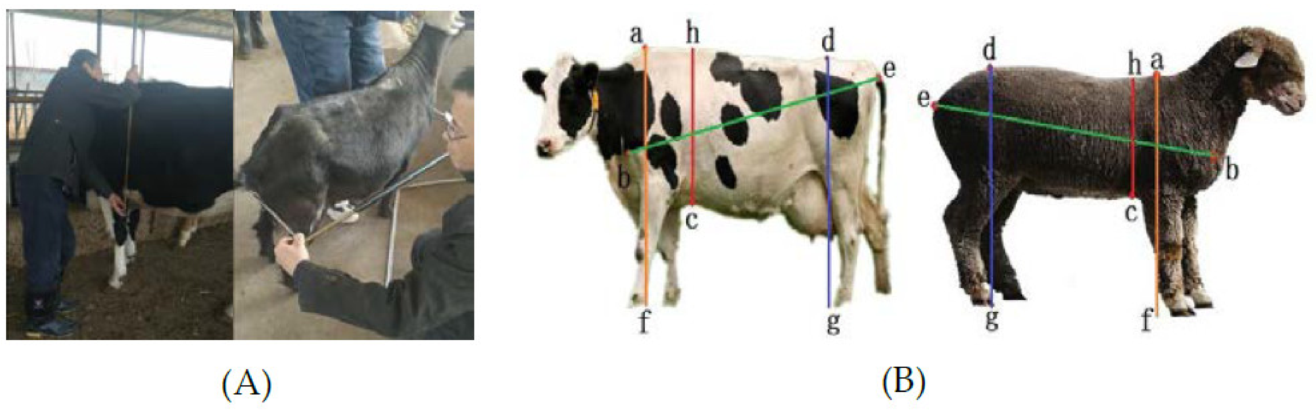
2.2. Nomentclature of Body Traits and Measurement

During the measurement, the height measuring instrument (the maximum measuring length, width and height are, respectively: 180 cm, 50 cm and 120 cm, while the instrument accuracy is one centimeter) was adopted to measure the body size of the cattle and goat, as shown in Figure 2A. The height measuring instrument was aligned to both sides of the feature points to obtain the length of the cattle and goat. In order to reduce the manual measurement error, two surveyors measured each cattle and goat three times. Finally, the average value was calculated as the final manual measurement result. All length data were in centimeters and one decimal place was reserved for all measurement results. Withers height, chest depth, hip height and body length should be measured [17,18], as shown in Figure 2B.

Above, a is the highest point of the withers, b represents the anterior extremity of the hummers, c is the shallowest part of the chest, d expresses the highest point of the hip bones, and e is the extremity of the ischium. The straight line a–f represents withers height, the vertical distance from the highest point of the withers to the ground surface at the level of the forelegs. The straight line c–h expresses chest depth. It is the vertical distance from the back to the shallowest part of the chest. The straight line d–g refers to hip height. It is the vertical distance from the highest point of the hip bones to the ground surface at the level of the hind legs. The straight line b–e denotes the body length; it is the distance from the anterior extremity of the humerus to the posterior internal extremity of the ischium.

2.3. Image Processing

The ultimate goal of image processing is to get the feature points of livestock in a color image, and then calculate the body size of livestock combined with a depth image. The workflow comprised: (1) depth image restoration. Resolution reconstruction of depth image was performed by combining color image and infrared image. We solved the effect of illumination and distance on the depth image, and reduced the texture copy artifacts in the depth image. (2) Set all image sizes to 768 × 768 pixels for data annotation and network training. The training set, validation set, and test set were divided according to the proportion of 5:3:2. (3) Body-part segmentation. Based on the optimized U-Net neural network, the remote, noncontact and automatic background segmentation and trunk segmentation of cattle and goat were realized, respectively. (4) Feature point location. We identified and located feature points through the multistage densely stacked hourglass network. None of the methods mentioned above use any pre-training network. The different steps are described in the subsections below.

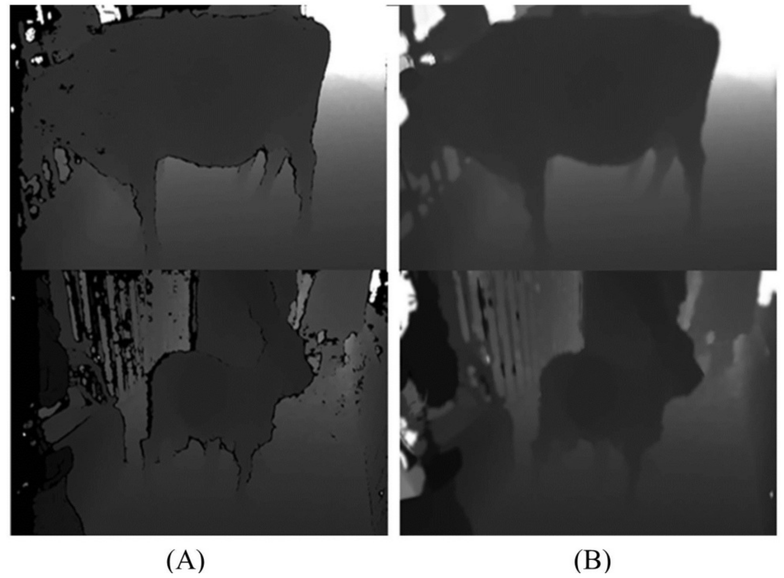
2.3.1. Depth Image Restoration

The depth camera is capable of collecting the depth information of the scene in real-time; however, illuminations, distances and other environmental factors significantly impact the quality of depth images [26,27]. To improve the robustness of distance and illumination and reduce the depth image texture and copy artifacts and depth discontinuity, this study proposed a depth image super-resolution reconstruction algorithm based on the autoregressive model. The algorithm consisted of data items and regular items, as expressed in the following equation. To be specific, the depth map D⁰ was obtained from the real depth image via the bicubic interpolation. “Ω” denotes the points in the depth image, and N(i) represents the points beside the point i in the depth image.

$$D=\arg {\min }_{D_i}\left\{{\displaystyle \sum _{i\in \mathsf{\Omega }}{‖D_i-D_i^0‖}_2^2}+\lambda {\displaystyle \sum _{\mathsf{\Omega }}\mathsf{\Phi }\left(D_i-{\displaystyle \sum _{j\in N\left(i\right)}{A}_{ij}{D}_i}\right)}\right\}$$

First, the penalty function $\mathsf{\Phi }\left(\mathrm{x}\right)$ was adopted to act on the regular term, as expressed below:

$$\mathsf{\Phi }\left(\mathrm{x}\right)=\frac{x}{e^{-x}+x}$$

$\mathsf{\Phi }\left(\mathrm{x}\right)$ denotes the M-estimator. As reported by Smoli [28], robust M-estimators could eliminate marginal uncorrelated patch. Figure 3 plots the L² penalty function curve and the penalty function curve applied in this study. The results indicated that the penalty function proposed in this study was capable of efficiently saturating in the iteration, making $\mathsf{\Phi }\left(\mathrm{x}\right)$ an approximation of L⁰ to keep the sharp edges of the image. Compared with the penalty function $\mathrm{G}\left(\mathrm{x}\right)=2\ast (1-\exp (-x^2/2\left)\right)$ applied in reference [29], the curve of $\mathsf{\Phi }\left(\mathrm{x}\right)$ achieved a faster saturation rate, so it would be more sensitive to outliers (e.g., noises and void).

Second, to increase the reconstruction effect of color images with unclear edges, the autoregressive coefficient ${\mathrm{A}}_{ij}$ is expressed as:

$${\mathrm{A}}_{ij}=\frac{1}{s}{A}_{i,j}^{D^0}F\left(A_{i,j}^C,A_{i,j}^I\right)$$

where $s$ denotes the normalization factor, the depth term $A_{i,j}^{D^0}$ was defined by the Gaussian filter, and the color term and the infrared term were, respectively, set as:

$$A_{i,j}^C=\exp \left(\frac{{\displaystyle {\sum }_{h\in c}{‖B_i^C\circ \left({\rho }_i^h-{\rho }_j^h\right)‖}_2^2}}{{\sigma }_1^2}\right)$$

$$A_{i,j}^I=\exp \left(\frac{{\displaystyle {\sum }_{h\in c}{‖B_i^I\circ \left({\rho }_i^h-{\rho }_j^h\right)‖}_2^2}}{{\sigma }_1^2}\right)$$

where ${\sigma }_1$ denotes the decay rate of the exponential function; ${\rho }_i^h$ represents the mask operator with the size $\omega \ast \omega$ centered on the pixel point within the color channel $h$. According to the extracted operators, the bilateral filter $B_i^C$ was adopted to adjust the distance and intensity difference.

$$B_i^C\left(i,j\right)=\exp \left(\frac{{‖i-j‖}_2^2}{{\sigma }_2^2}\right)\exp \left(-\frac{{\displaystyle {\sum }_{h\in c}\left(C_i^h-C_j^h\right)}}{{\sigma }_2^2}\right)$$

The filters $B_i^C$ employed a bilateral kernel to weigh the distance of the local patch. Compared with the Gaussian kernel adopted by the standard filter, the color term and the infrared term showed a strong response to the pixels $x$ with similar results. Accordingly, the regression prediction of image edge pixels was significant.

Lastly, the check function $F(x)$ was introduced in the regular term, as expressed below:

$$F(x)=\left\{\begin{array}{c}{A}_{i,j}^C,LBP\left(C\right)\ge LBP\left(I\right)\\ A_{i,j}^I,LBP\left(C\right)\prec LBP\left(I\right)\end{array}\right.$$

To be specific, $LBP\left(x\right)$ represents an operator proposed by Ojala et al. [30] to describe the local texture features of images; it is defined in 3 × 3 windows, while the value of 8 adjacent pixels was compared with the threshold value of the center pixel of the window. If the surrounding pixel value was greater than the central pixel value, the position of the pixel was marked as 1, but otherwise was 0. In this way, the LBP operator of the central pixel of the window could be obtained, and this value could be used to reflect the texture information of the region. The process was shown in Figure 4.

In this study, the LBP equation is written as follows: $LBP\left(C\right)$ represents the $\rho$ sampling point in the circular area; $R$ is the radius of the circular area; $G\left(m\right)$ expresses the gray value of the central pixel, and $G\left(p\right)$ denotes the gray value of the $\rho$ circular boundary pixel.

$$LB{P}_{\mathrm{P},\mathrm{R}}\left(x_c,y_c\right)={\displaystyle \sum _{n=1}^{\rho }s\left(G\left(\rho \right)-G\left(m\right)\right)\ast 2\rho }$$

Thus, in the regular term, the LBP function was adopted to judge the edge features of the color image and the infrared image, a high-quality mask operator was selected to act on the super-resolution model of the depth image. The effect of illumination and distance on the depth image was solved effectively. The texture copy artifacts and the depth discontinuities decreased significantly. Figure 5 gives the super-resolution result of depth image.

In the real-world experiment, since there were no standard depth maps as reference, Peak Signal-to-Noise Ratio (PSNR) and Structural Similarity (SSIM) could not be used to measure the quality of image reconstruction. In order to further verify the effectiveness of this method, Mean Gradient (MG) and Laplace Operator (LO) [31] were selected as evaluation indexes in this study. The higher MG and LO values were, the better image quality was. The formula of MG was as follows:

$$\begin{array}{l}MG=\frac{1}{(M-1)(N-1)}\ast \\ {\displaystyle \sum _{i=1}^{M-1}{\displaystyle \sum _{J=1}^{N-1}\sqrt{\frac{{\left(F(i,j)-F(i+1,j)\right)}^2+{\left(F(i,j)-F(i,j+1)\right)}^2}{2}}}}\end{array}$$

In the formula, the gray value of row $i$ and column $j$ in the image was expressed as $F(i,j)$; M and N were the total number of rows and columns of the image. The encapsulation method of Laplace Operator was provided in OpenCV, which could be called directly. The formula of LO was as follows:

$$\mathrm{L}O={\displaystyle \sum _x{\displaystyle \sum _y\left|G(x,y)\right|}}$$

The results were shown in Section 3.

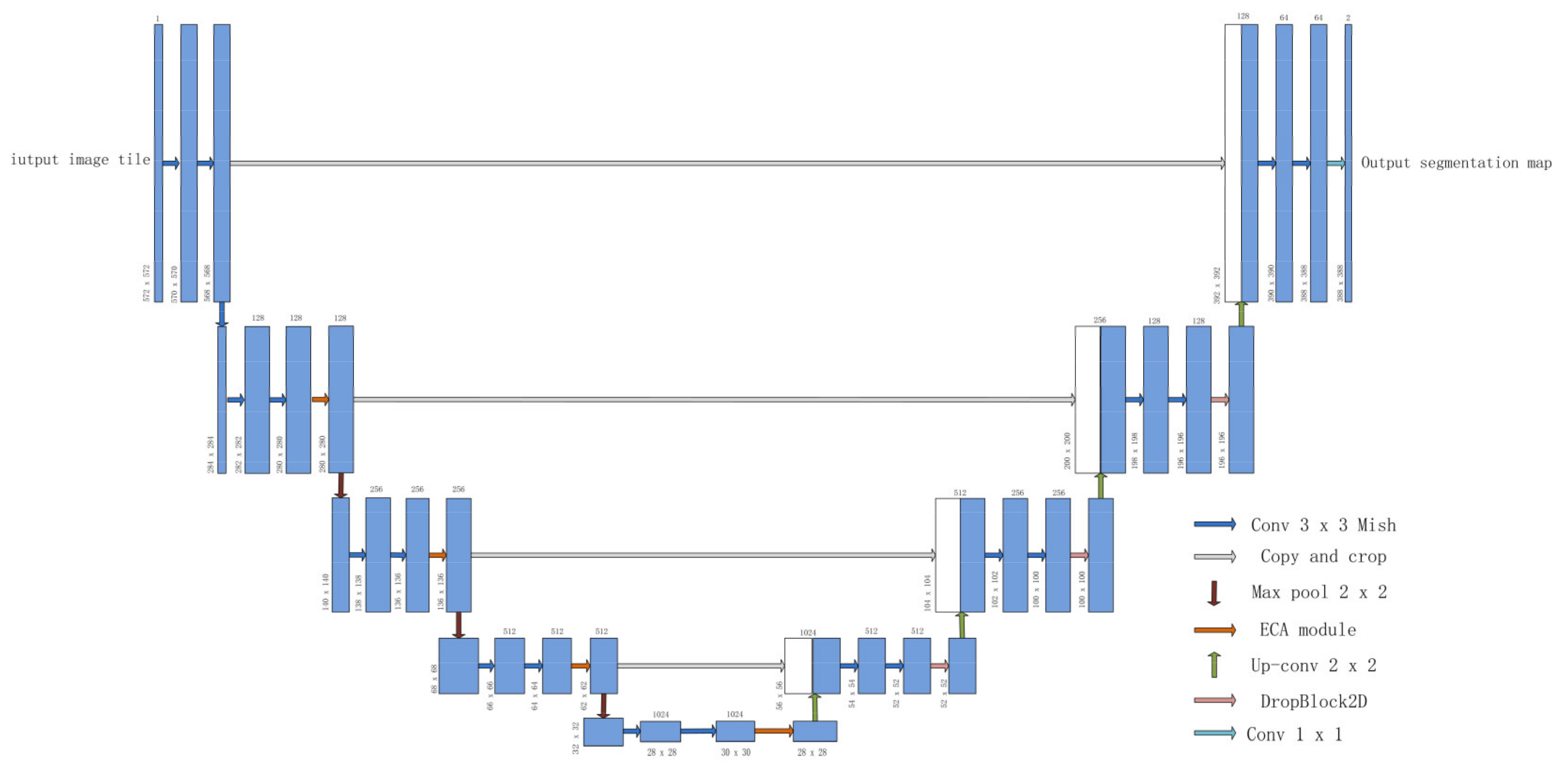
2.3.2. Body-Part Segmentation

To improve the accuracy of the semantic segmentation in complex backgrounds and reduce the segmentation error in up sampling, this study optimized the U-Net neural network model based on PyTorch framework (Version 1.5.0) to achieve a remote, noncontact and automatic detection of vital positions of cattle and goats, respectively. Figure 6 shows the model.

First, the U-Net neural network employed ReLU as the activation function. Since the negative semi-axis value of ReLU was always zero, when the model inputted the minimum value, the neuron would die because it was not activated. To solve the gradient disappearance attributed to the ReLU activation function, the ReLU activation function after each convolutional layer and Batch Normalization layer in the U-Net neural network was replaced with the Mish activation function. The function of Mish and ReLU are illustrated in Figure 7.

Since the positive semi-axis derivative of the Mish was greater than 1, it avoided the saturation because of the function capping, while preventing the gradient from disappearing. The negative semi-axis of the Mish was not always zero, whereas it remained a small value, which solved the problem of neuron death; moreover, Mish improved the sparse expression of the network and addressed the gradient disappearance attributed to the lack of training data and the increase in network layers. According to existing studies, a smooth activation function can more effectively allow the information to penetrate the neural network [32]. Better generalization results can be achieved since the Mish is smoother than that of ReLU.

Second, this method introduced the attention mechanism to increase the accuracy of semantic segmentation. The attention mechanism refers to a data processing method in machine learning, originating from natural language processing. Relevant researchers suggested that avoiding dimension reduction helps learn effective channel attention, and appropriate cross-channel interaction is capable of reducing model complexity while keeping performance [33].

Accordingly, the model could add the attention mechanism module after the respective down-sampled convolution module. First, the binary adaptive mean method was adopted to calculate and pool the input data to a size of 1 × 1. After the global average pooling, the 1D convolution with weight sharing characteristics was exploited to capture the cross-channel interaction information. Next, the nonlinear relation was introduced through the sigmoid activation function. Lastly, the result was multiplied by elements and then expanded into the same dimension as the input data, so the dimension of the data processed by the attention mechanism module remained unchanged. By introducing the attention module, the accuracy of semantic segmentation tasks was significantly improved. Figure 8 presents the attention mechanism module.

Lastly, to achieve the desired segmentation effect more accurately and efficiently, the method added the DropBlock2D module during each up sampling. The DropBlock module [34] refers to a regularization module for the convolutional neural network. The effect is illustrated in Figure 9. Such a module removed an area around a feature and forced the network to learn other features of the object after multiple iterations of training.

After processing by the neural network model proposed in this study, the background and body feature regions of cattle and goats could be effectively segmented. The segmentation effect is given in Figure 10.

To further verify the effectiveness of the method, LabelImg was used to manually annotate the images to obtain the real segmentation. Fifty images of cattle and goats were randomly adopted from the test set, respectively, and the accuracy, the sensitivity, the specificity and the dice similarity coefficient (dice) [35,36] were employed to assess to the effect of the body-part segmentation method.

$$Accuracy=\frac{TP+TN}{TP+FP+TN+FN}$$

$$Sensitivity=\frac{TP}{TP+FN}$$

$$Specificity=\frac{TN}{TN+FP}$$

$$\mathrm{d}ice=\frac{2\ast TP}{\left(TP+FN\right)+\left(TP+FP\right)}$$

where TP represents the number of body-part pixels correctly identified as body-part segmentation method compared to the real segmentation by LabelImg. FP represents the number of body-part pixels correctly identified as Body-part segmentation method compared to the pixels as non-body parts identified by LabelImg. TN represents the number of body-part pixels incorrectly identified as the body-part segmentation method compared to the pixels as non-body parts identified by LabelImg. FN denotes the number of body-part pixels incorrectly identified as body-part segmentation method compared to the real segmentation by LabelImg.

Since Dice is sensitive to internal filling, Hausdorff distance (HD) [37,38] is introduced to evaluate the segmented boundary.

$$\mathrm{HD}\left(\mathrm{A},\mathrm{M}\right)=\max \left\{\underset{}{\underset{i}{\max }\left[d\left(a_i,M\right)\right],\underset{}{\underset{j}{\max }\left[d\left(m_j,A\right)\right]}}\right\}$$

where $\mathrm{A}=\left\{a_1,a_2,a_3\dots a_i\right\}$ represents the result point set segmented by automatic, and $\mathrm{M}=\left\{m_1,m_2,m_3\dots m_j\right\}$ represents the result point set segmented by manual. $a$ and $m$ were points on the boundary respectively. $d\left(\mathrm{x},y\right)$ is the Euclidean distance from $\mathrm{x}$ to $y$. The results were shown in Section 3.

2.3.3. Feature Point Location

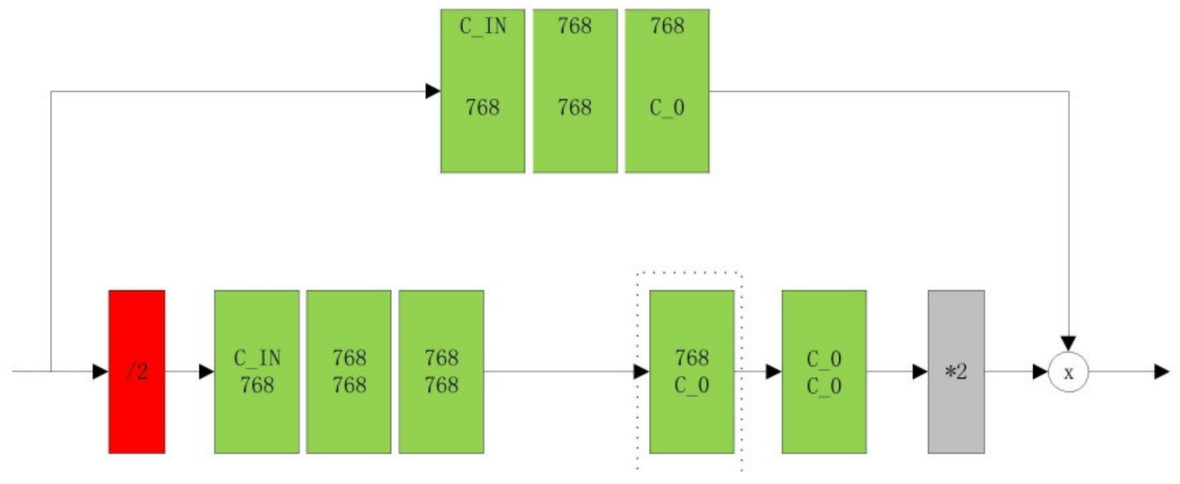
Feature point location refers to a vital research field in the computer vision. Over the past few years, studies such as the human body joint point location [39,40,41] and the face key point location [23,42,43] have shown that on the premise of sufficient data, deep learning could extract better features compared with the manual construction of features. This research solved the problem that traditional methods could not accurately locate livestock feature points by created a multistage densely stacked hourglass network.

Dense Block

The stacked hourglass network comprises residual blocks. In this study, dense blocks [44] were selected to replace residual blocks. Compared with residual blocks, dense block networks exhibited a simple structure and fewer parameters than ResNet. Second, dense blocks could send information between any two layers, thereby enhancing the reuse of features and alleviating the problems of gradient vanishing and model degradation.

In a dense block, any two layers were connected to each other. The input of each layer in the network was the output of all previous layers, and the feature map learned by this layer would act as the input of the later network layer. The dense block structure is expressed as $x_n=h_n\left([x_0,x_1,x_2\dots x_{n-1}]\right)$, where $x_n$ denotes the input of the layer n, $[ ]$ represents splicing, combining all output feature graphs from $x_0$ to $x_{n-1}$ layers according to channels, and $h_n$ expresses a composite function (i.e., Batch Norm, activation function and a 3 ∗ 3 convolution).

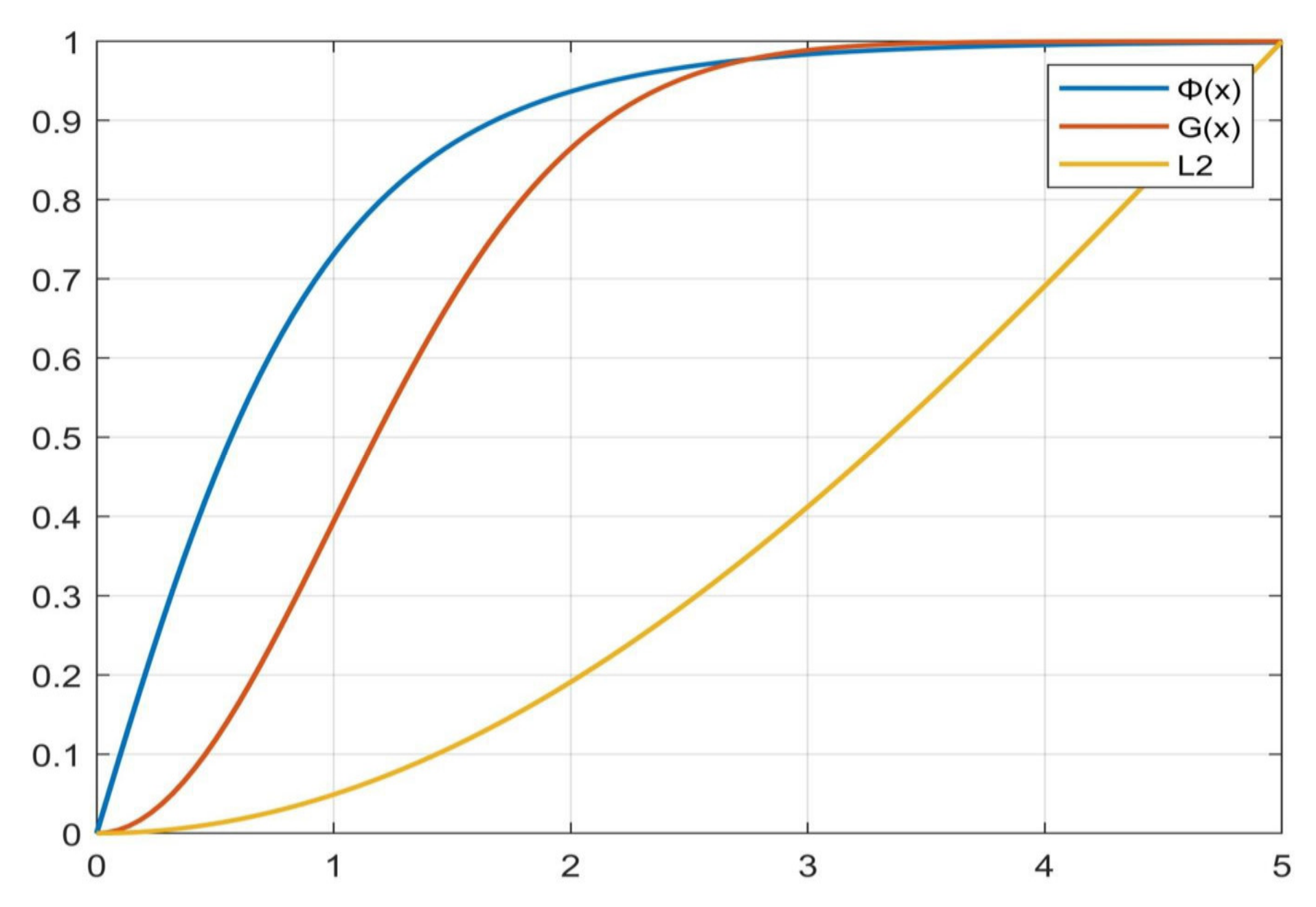
Objective Function Optimization

The stacked hourglass network used the mean square error loss (L² loss function) as the loss function, and the calculation equation is written as: $S={\sum }_{i=1}^n{(Y_i-f(x_i\left)\right)}^2$. The L² loss function caused the model to produce a greater loss at the noise point. When the model optimized the loss of noise points, the performance of the model would be reduced; thus, this study adopted the Huber loss function to replace the original loss function to reduce the sensitivity of the network to noise points and endow the network with a better generalization capability. The Huber loss function equation is presented below:

$$L_{\delta }(y,f\left(x\right))=\left\{\begin{array}{c}\frac{1}{2}{\left(y-f\left(x\right)\right)}^2\\ \delta \left|y-f\left(x\right)\right|-\frac{1}{2}{\delta }^2\end{array}\right.$$

The Huber loss is essentially an absolute error, only becoming a squared error when the error was small. The hyper parameter $\delta$ was used to control when it became a quadratic error. When the value of the Huber loss function was in the interval [0 − $\delta$, 0 + $\delta$], the Huber loss function was equal to mean square error. When the value of Huber loss function was in the interval [−$\infty$, $\delta$] or the interval [$\delta$, + $\infty$], the Huber loss function was equated with Mean Absolute Error. Accordingly, the Huber loss function combined the advantages of MSE and MAE, and it would be more robust to abnormal points.

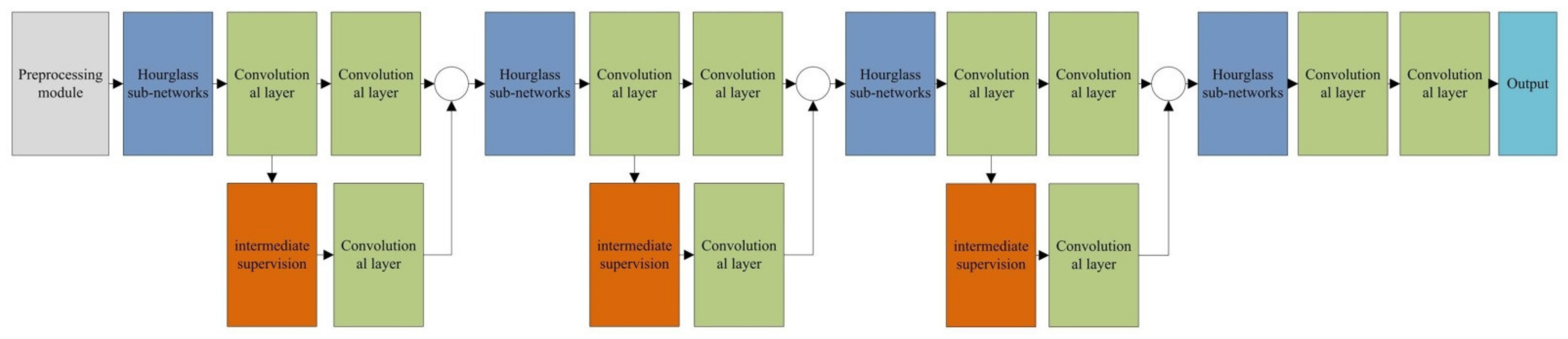
Multistage Densely Stacked Hourglass Network

Accurate positioning of the pixel position of the feature points of the livestock is of great significance to improve the accuracy of the livestock size measurement. In recent years, deep learning technology has been widely used, but there was little research on feature point location of livestock. Referred to the idea of human feature points location based on deep learning [45,46], this study used multistage densely stacked hourglass network to locate the feature points of livestock.

The stacked hourglass network mainly consisted of hourglass sub-networks, and Figure 11 illustrates the hourglass network. The upper and lower halves of the graph contain several light green dense blocks to gradually extract deeper features. Dense blocks were mainly composed of residual modules. The step and padding of all convolution layers for all residual modules were set to 1. All operations did not change the data size; they only changed the data depth (channel). The value C_IN in the first row of the dense block represents the number of channels of the input image, and that in the second row represents the number of output channels. The red module represents the down sampling layer, using the max pooling method. The gray module represents the upper sampling layer, using the nearest neighbor interpolation method. The dashed box could increase the order of the network by splicing other hourglass sub-networks.

The multistage densely stacked hourglass network refers to a serial stack of hourglass sub-networks; however, with the increase in the network depth, the parameters increased, making it difficult to perform effective training updates. To solve such a problem, this study adopted the relay supervision strategy in the model for the supervised training. The experiments in this study were all performed on a three-stage stacked hourglass network. Figure 12 gives the four-level densely stacked hourglass network.

After the original image was preprocessed, the scale information of the image was preserved for the next layer of feature fusion. In addition, the preprocessed image was input into the hourglass sub-networks for a down sampling operation. After three residual modules and two convolution modules, the features were extracted step by step, and the feature map of the layer was obtained through the up-sampling operation. At the same time, after up sampling operation, the scale information of the upper layer was fused and used as the input of the next hourglass sub-networks to extract the features.

This study adopted the PyTorch framework for training, the input image was a color image with a resolution of 768 × 768, and the number of iterations was set to 16,000. The training set, validation set, and test set were divided according to the proportion of 5:3:2. For every 10,000 steps, the learning rate declined to 10%. Moreover, to increase the convergence speed, the normalization operation was added to the model.

2.4. Evaluation of Body Size Measurement

Withers height, hip height, body length and chest depth of 13 cattle and 10 goats were measured manually and automatically. The absolute error, relative error, linear regression and repeatability have been used to verify the validity of the body size measurement method.

First, the absolute error was used to reflect the deviation between automatic measurement and manual measurement. Since the absolute error and the measured value have same unit, the relative error was introduced to compare the reliability of the automatic measurement.

Second, the ideal relationship between manual measurement and automatic measurement should be Y = AX while A = 1. This research used linear regression to fit the relationship between manual measurement and automatic measurement. The effectiveness of the measurement method was verified by coefficient of determination and RMSE. A high coefficient of determination R² determination represented a good fit. RMSE was used to reveal the typical distance between predicted value made by the regression model and the actual value.

Finally, for the repeatability evaluation of the measurement method, the researchers often used the intraclass correlation efficient (ICC) to assess the similarity of a quantitative attribute among individuals and to assess different measurement methods or assess the repeatability of the same measurement result by the observer [47]. Measurement experiments generally employed ICC to assess the repeatability of different measurement methods to the same target [12]. The precondition of this study was that the manual measurement was considered to be the most reliable and repeatable; thus, we just assessed the repeatability of automatic measurement to the target by ICC and Coefficient of Variation (CV).

3. Results and Discussion

3.1. Depth Image Restoration

Ten depth images of cattle and goats and their corresponding color images and infrared images were randomly selected from the data set. Joint Bilateral Upsampling (JBU) [48], Weighted Least Squares (WLS) [49], Autoregressive Model (AR) [50] and the algorithm proposed in this research were used to reconstruct the depth images, respectively. The results are shown in

Table 1. Comparison of MG and LO values of reconstruction results.

		Goat	Cattle
	MG	LO	MG	LO
JBU	0.0027	22.646	0.0028	21.404
WLS	0.0029	21.967	0.0029	22.142
AR	0.0032	74.482	0.0032	86.814
Ours	0.0048	142.170	0.0050	154.748

.

The results showed that the depth image reconstruction effect of AR algorithm was better than JBU algorithm and WLS algorithm, but there were still deep texture copy artifacts in the reconstructed depth image. In this research, making full use of the texture features of infrared image could greatly improve the reconstruction quality of depth images. The effect of illumination and distance on the depth image was solved effectively. The texture copy artifacts and the depth discontinuities decreased significantly. Compared with other algorithms, our method improved both visual effect and image quality.

3.2. Body-Part Segmentation

The cattle and goat body segmentation contains front trunk segmentation, central body segmentation and hip–torso segmentation. The average of accuracy reached 93.68% and 93.50%, the sensitivity was 71.65% and 68.90%, and the specificity was 97.78% and 97.97%, respectively (

Table 2. Body-part detection performance parameters for side view of cattle (%) *.

Index	Background	Front Trunk	Central Body	Hip Torso	p-Value
Accuracy	97.09 ± 1.56 a	94.30 ± 1.53 b	95.33 ± 1.70 ab	89.55 ± 1.29 c	<0.001
Sensitivity	89.29 ± 1.11 a	54.55 ± 1.63 d	80.00 ± 1.26 b	71.43 ± 1.02 c	<0.001
Specificity	99.57 ± 0.60 a	99.75 ± 0.60 a	97.83 ± 0.57 b	94.34 ± 0.64 c	<0.001
Dice	93.67 ± 0.71 a	69.76 ± 0.66 b	82.75 ± 0.54 c	74.07 ± 0.79 d	<0.001

* All data were presented as average ± SD. One-way analysis of variance (ANOVA) followed by Turkey’s multiple-range test was used to determine significant differences among different segmentations. Different superscript letters indicate significant differences (p < 0.05).

and

Table 3. Body-part detection performance parameters for side view of goats (%) *.

Index	Background	Front Trunk	Central Body	Hip Torso	p-Value
Accuracy	96.73 ± 0.95 a	95.27 ± 0.85 b	95.52 ± 1.09 b	87.59 ± 1.16 c	<0.001
Sensitivity	90.00 ± 1.39 a	60.98 ± 1.29 c	76.92 ± 1.15 b	60.81 ± 1.24 d	<0.001
Specificity	99.40 ± 0.62 a	99.26 ± 0.61 a	98.23 ± 0.63 b	95.13 ± 0.69 c	<0.001
Dice	92.99 ± 0.89 a	72.88 ± 0.83 b	81.38 ± 0.49 c	68.28 ± 0.91 d	<0.001

* All data were presented as average ± SD. One-way analysis of variance (ANOVA) followed by Turkey’s multiple-range test was used to determine significant differences among different segmentations. Different superscript letters indicate significant differences (p < 0.05).

). For background segmentation of cattle and goat, the accuracy reached 97.09% and 96.73%, the sensitivity was 89.29% and 90.00%, the specificity was 99.57% and 99.40%, and the dice similarity coefficient was 93.67% and 92.99%, respectively (Table 2 and Table 3). The Hausdorff distances of background segmentation between cattle and goat were 5.93 mm and 6.16 mm, respectively (

Table 4. Hausdorff distance of body segmentation between cattle and goat (mm).

Index	Cattle	Goat
Background	5.93 ± 1.38	6.16 ± 1.41
front trunk	6.74 ± 1.56	6.94 ± 1.49
central body	6.23 ± 1.12	6.78 ± 1.23
Hip torso	7.37 ± 1.74	8.40 ± 1.77

). Compared to background segmentation, body segmentation required further segmentation in a smaller segmentation area and a more similar color background, which might lead to a relatively worse effect of body segmentation than background segmentation. For body segmentation, the hip torso was a significantly poor segmentation effect compared to front trunk segmentation and central body segmentation. As impacted by the low sensitivity of the segmentation method to the tails of cattle and goats, the tails and trunks of livestock could not be separated from the background.

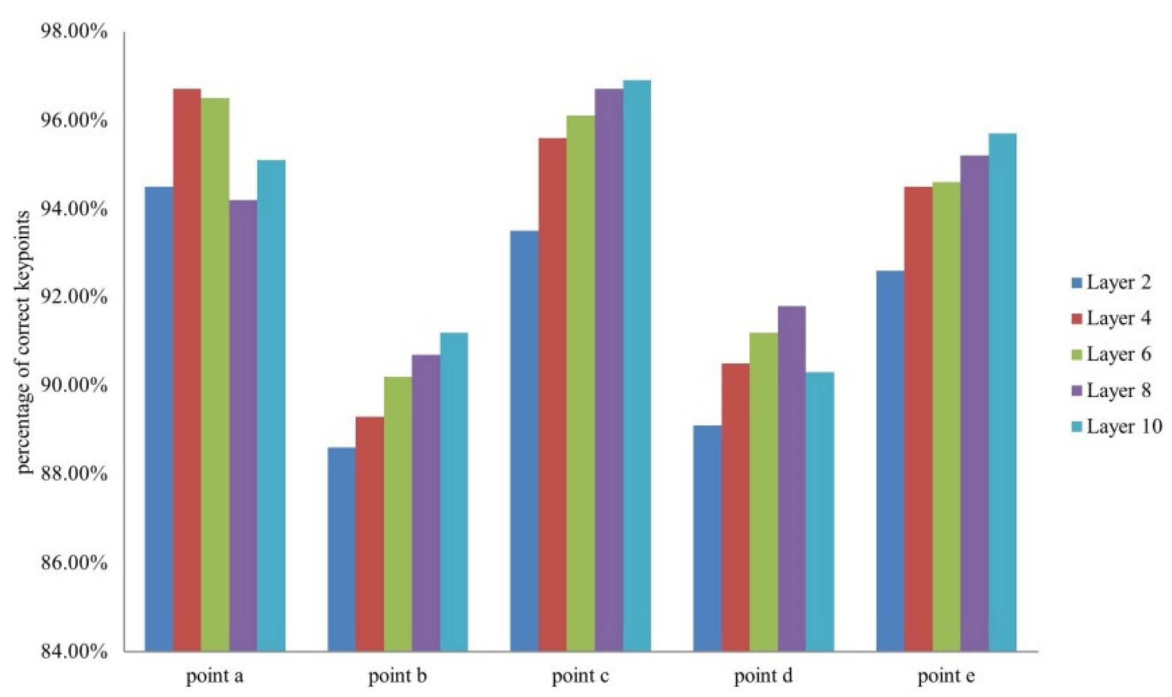
3.3. Accuracy of Feature Point Location

This study selected 2, 4, 6, 8 and 10 dense hourglass blocks for testing. Figure 13 shows the experimental results. To be specific, a–e represents the quantitative feature points of cattle and goats marked in Figure 2.

Evaluation used the percentage of correct key points ($\sigma =0.5$) [39,51] metric which reports the percentage of detections that fall within a normalized distance of the ground truth. In this study, because some pictures did not collect the head information of livestock, the body length of livestock was selected to calculate the normalized distance between the predicted feature point and the real feature point.

This study used the self-built data set to train the multistage densely stacked hourglass network. The evaluation reported that the model exhibited high universality and could accurately locate the feature points of cattle and goats. Figure 14 presents the location effect.

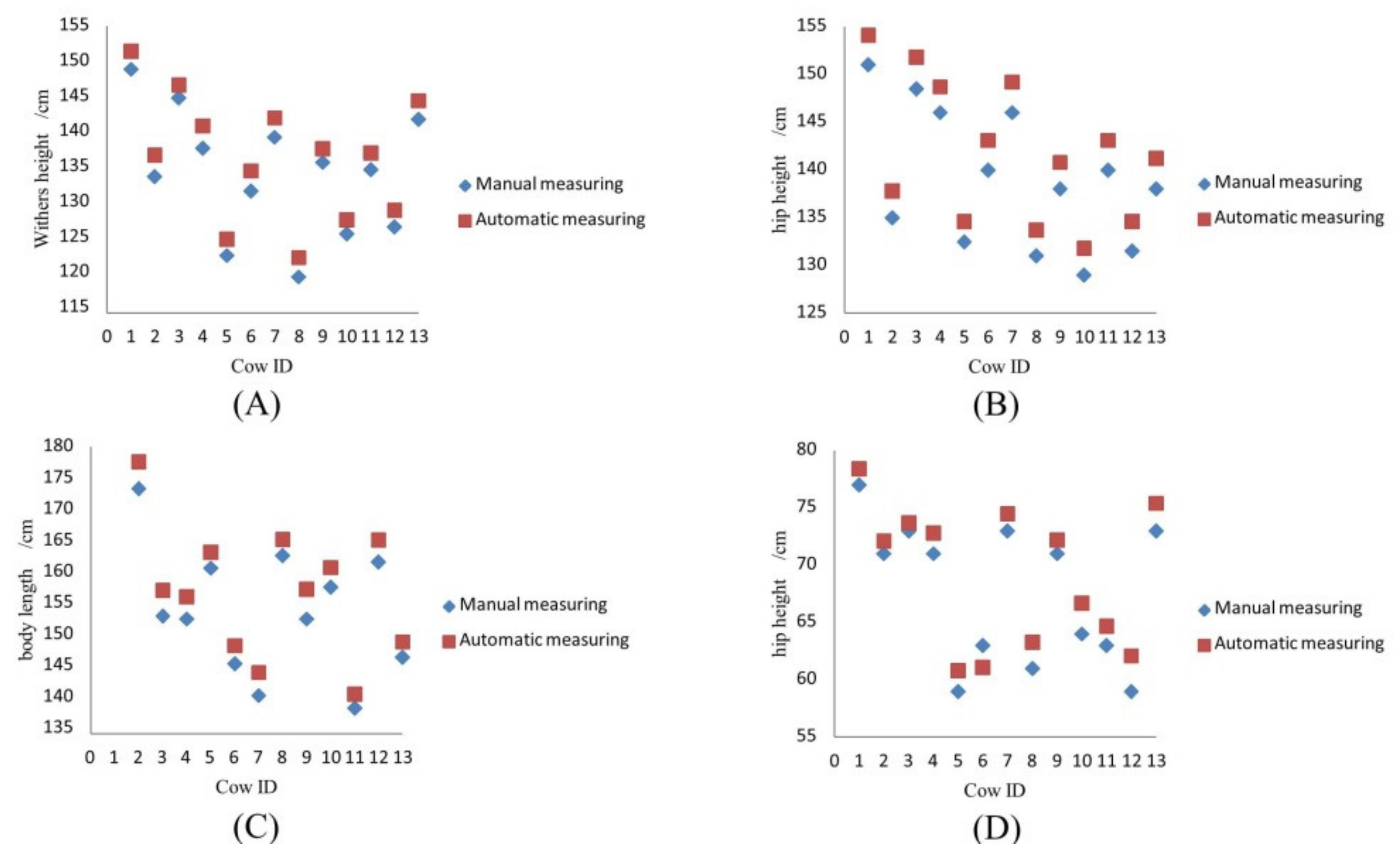
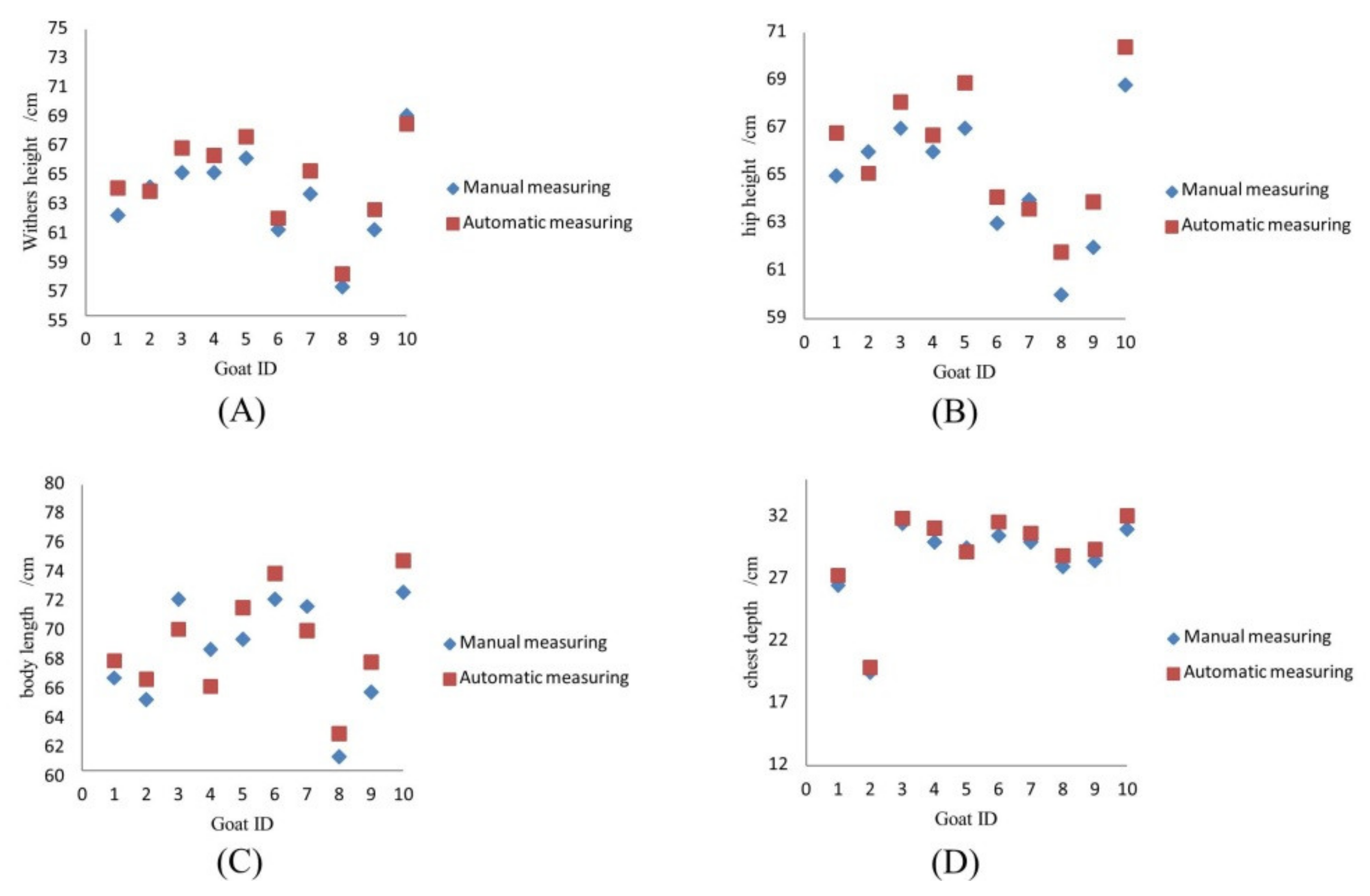
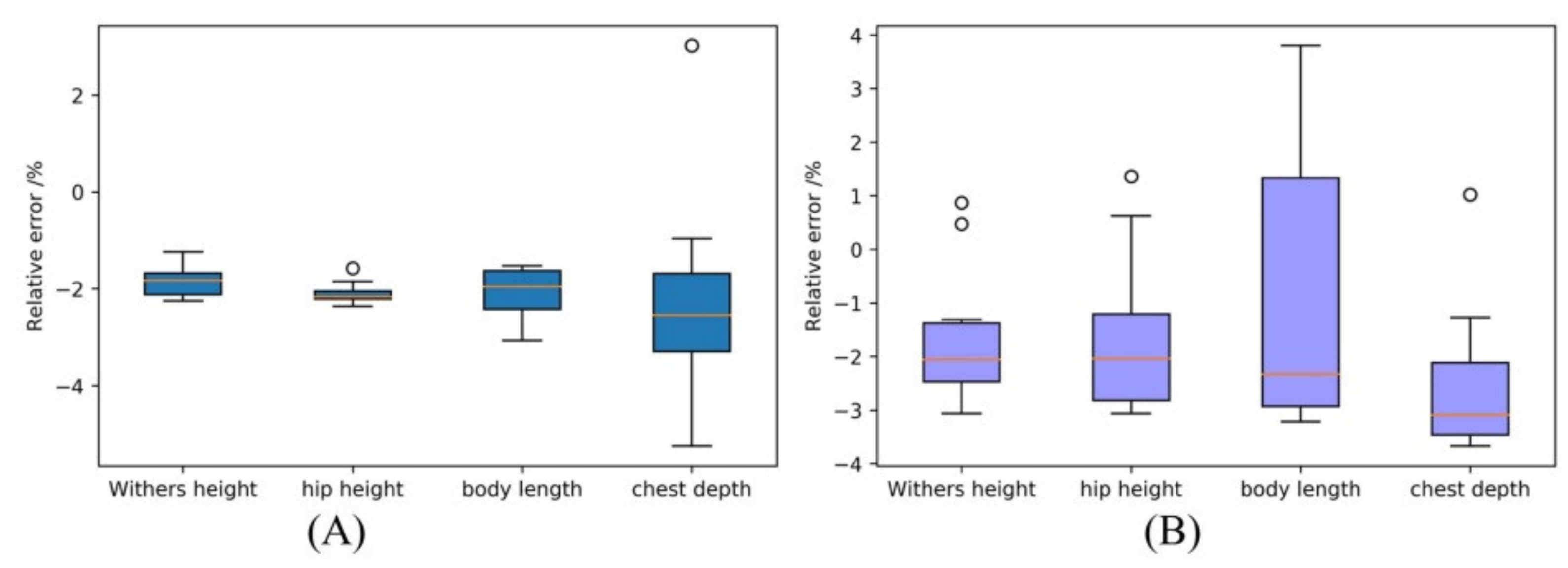
3.4. Accuracy of Measurement

According to Figure 15 and Figure 16, most automatic measurement results were greater than the manual measurement results. Given the Biltmore stick clings to livestock torso and less affected by the livestock fur during manual measurements, the livestock fur greatly affected the background segmentation and the feature point location. The method located feature points were close to fur of the livestock, but not close to body. The result of the automatic measurement was slightly greater than that of the manual measurement.

The box plots of the absolute error and relative error between manual measurement and automatic measurement were shown in Figure 17 and Figure 18. The average absolute error of withers height, hip height, and chest depth were mostly between 1 and 2 cm, and most accuracies of withers height were greater than hip height, body length and chest depth. The body length had the largest average absolute error, which may because the shoulder point (point b in Figure 2) was located at the front edge of the shoulder, greatly affected by the animal’s posture. Moreover, the color and depth of the feature points were similar to those of the surrounding pixel points, resulted the great error in body length measurement. The mean relative errors of withers height, hip height, body length and chest depth were 0.68%, 0.68%, 1.39% and 1.60% for cattle, and 0.65%, 1.06%, 1.77% and 1.99% for goat, respectively. The average relative error of the measurement results was between −2% to 2%; therefore, the results of the automatic measurement could be trustworthy in terms of the measurement accuracy.

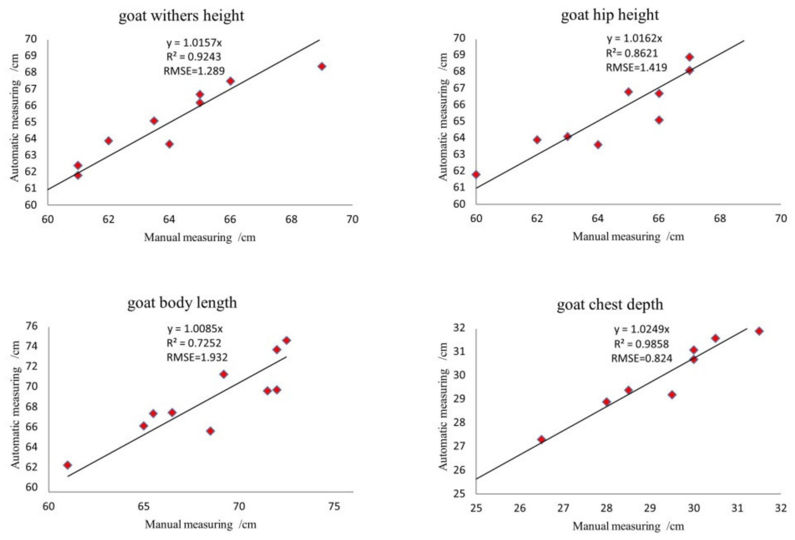
3.5. The Linear Regerssion Analysis of Measurement Results

As shown in Figure 19, the coefficient of determination of withers height, hip height body length and chest depth of cattle were 0.9974, 0.9985, 0.9954 and 0.9579, and RMSE were 2.492, 2.939, 3.328 and 1.927, which demonstrated that the two variables had a high degree of explanation. The linear regression coefficient of the cattle body size measured was close to 1, which showed the consistency of automatic measurement with the manual measurement.

As shown in Figure 20, the coefficient of determination of withers height, hip height body length and chest depth of goats were 0.9974, 0.9985, 0.9954 and 0.9579, and RMSE were 1.289, 1.419, 1.932 and 0.824. The coefficient of determination of automatic measurement was slightly lower than cows. Since goats are smaller than cattle, it is difficult to locate the feature points. In fact, whether it is automatic measurement or manual measurement, when the size of livestock decreases or the bone is unclear, the accuracy of feature point location will decrease [52]; however, the linear regression coefficient of the goats’ body size measured was close to 1, which showed the consistency of two measurement methods.

3.6. Repeatability of Measurement Results

Table 5. The analysis results of repeatability and reproducibility *.

	ICC		CV
	Cattle	Goat	Cattle		Goat
			Manual	Automatic	Manual	Automatic
withers height	0.990	0.985	0.064%	0.065%	0.052%	0.054%
hip height	0.985	0.943	0.052%	0.049%	0.041%	0.043%
body length	0.973	0.890	0.068%	0.069%	0.056%	0.064%
chest depth	0.972	0.942	0.091%	0.090%	0.123%	0.141%

* ICC describes the reliability and repeatability of measurements for clusters. The value of ICC close to 1 indicates high reliability and repeatability. CV is a normalized measure of the dis-persion of probability distribution, which is defined as the ratio of standard deviation to average.

lists the repeatability and reproducibility analysis results of this study after ten measurements. The value of ICC was between zeros to one. If the value of ICC was less than 0.4, the repeatability of the experiment would be poor; if the value of ICC was greater than 0.75, the experiment would exhibit better repeatability. In this study, the ICC of all body measurements was greater than 0.9, thereby showing good measurement repeatability. The ICC of withers height and hip height of cattle and withers height of goats all exceeded 0.980, which demonstrated higher reliability than other. Using the automatic measurement to measure body size of cattle, the value of CV ranged from 0.049% to 0.090% (variance ranges from 6.91 cm to 10.83 cm). The range of CV for goat body measurements ranged from 0.043% to 0.141% (variance ranges from 2.79 cm to 4.43 cm). According to Fischer, measurement methods with the repeatability and reproducibility had a CV less than 4%, as in the present study were considered promising [53].

Table 5 lists the body size measurement result of cattle, better than that of goats. Besides the effect of fur, another reason was that during the depth data collection, the behaviors of goats were more active than cattle; therefore, the distance between livestock and depth camera is not consistent. In many goat images, the area occupied by the torso is smaller than that of cattle; thus, there were more holes and texture copying artifacts in the depth images. The mentioned holes and texture replication artifacts would exist around the feature points, and would also affect the background segmentation and feature point extraction even after the depth image super-resolution reconstruction.

4. Conclusions and Future Studies

This study proposed a livestock body size measurement method and could measure various livestock body sizes under different backgrounds, respectively. The innovation of this method mainly includes the following:

(1)

Based on autoregressive models, a new penalty function was used to complete depth image super-resolution reconstruction through the color image and infrared image as guide image. The effect of illumination, distance and other factors on the quality of depth images was reduced.

(2)

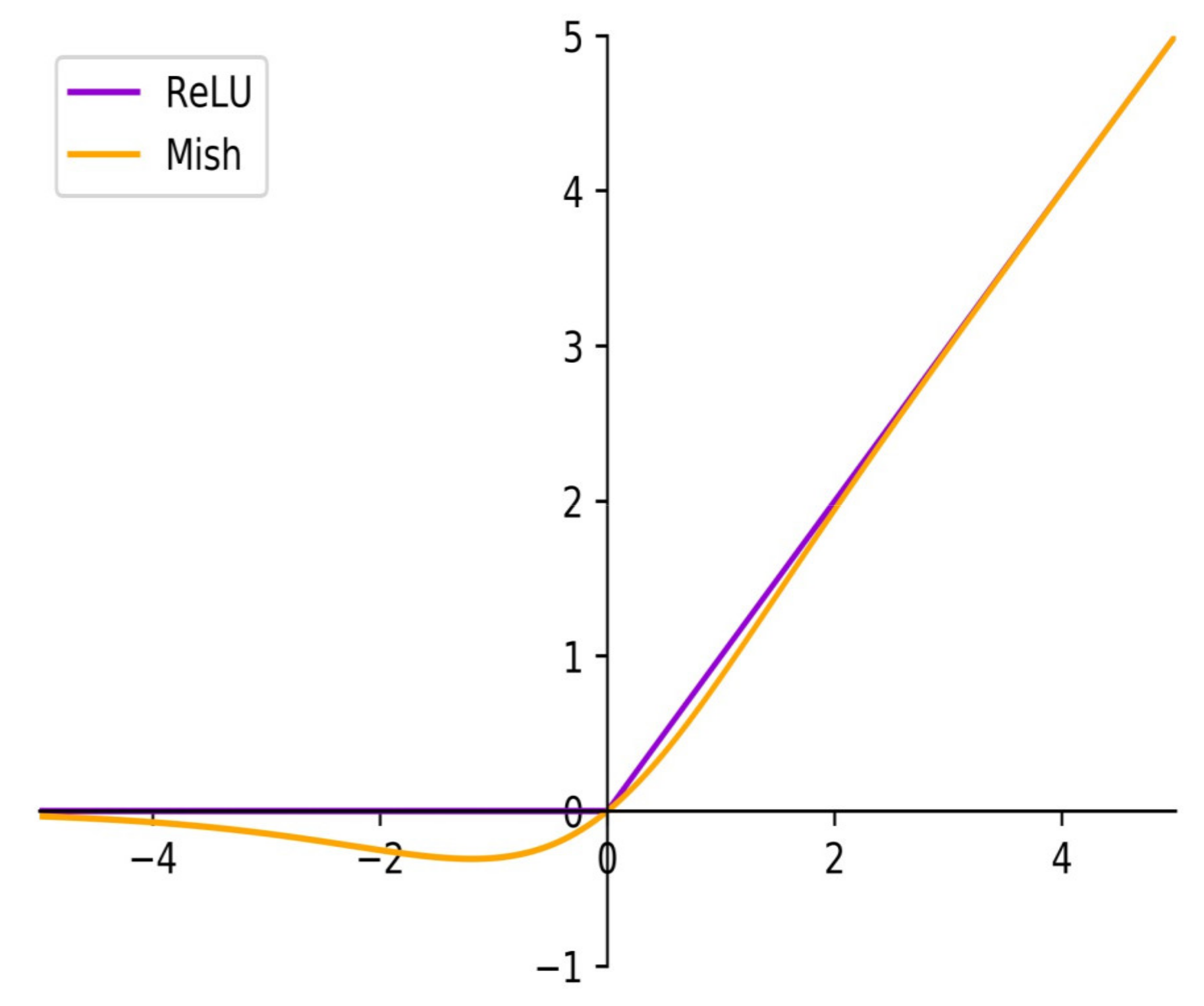
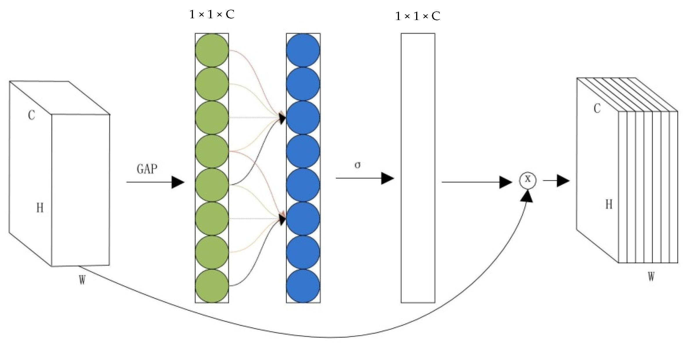
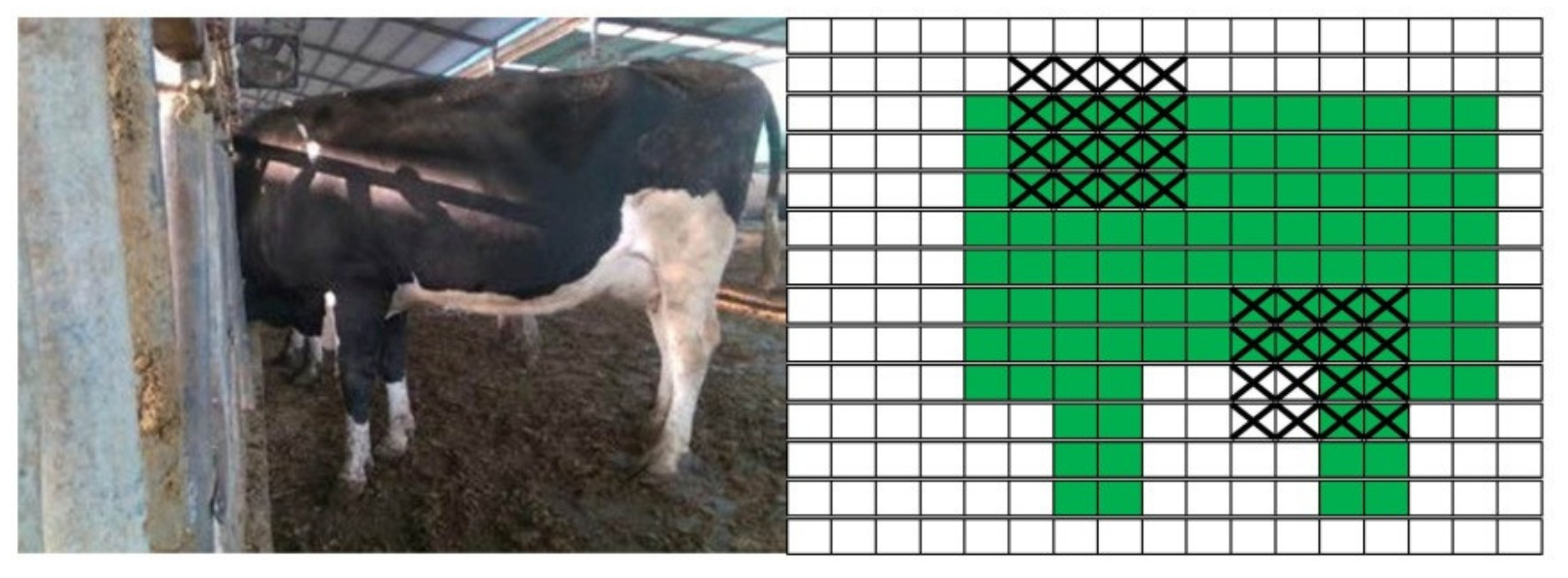
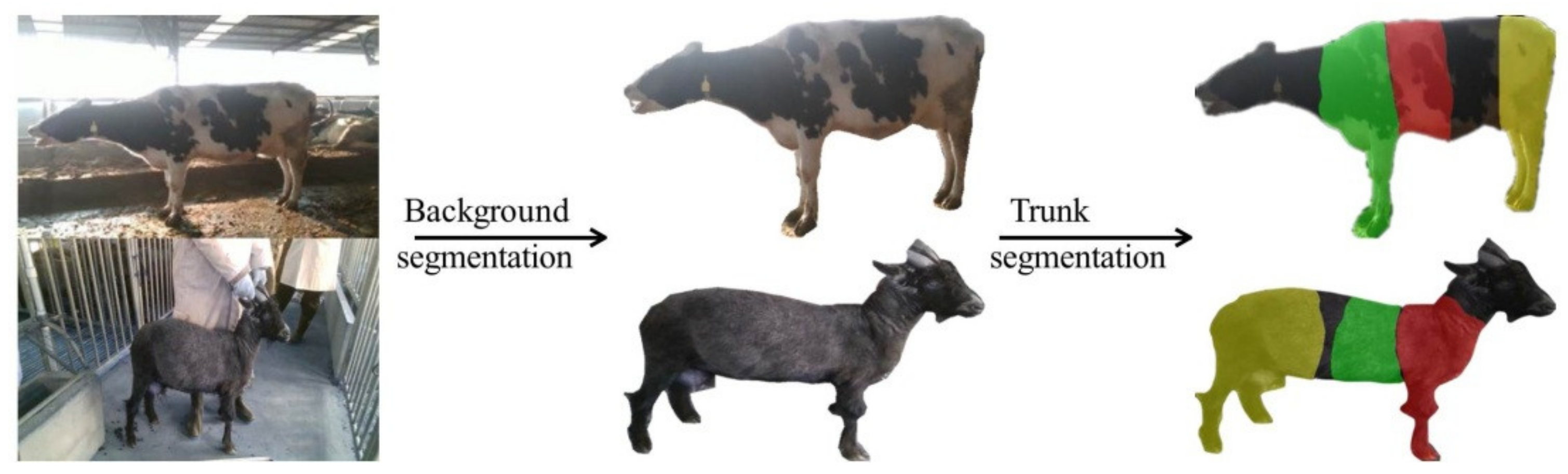
Combining the characteristics exhibited by the attention module and the DropBlock2D module, this study used a self-built database to realize remote, contactless, automatic background segmentation and trunk segmentation of cattle and goats, respectively, by optimizing the activation function of U-Net neural network.

(3)

It was the first time to use deep learning technology to locate livestock feature points. The three-stage stacked hourglass network was constructed by optimizing the objective function;l moreover, the relay supervision strategy was applied for the supervised training to achieve the feature point location of cattle and goats.

The results showed that the average accuracies of cattle and goat body segmentation were 93.68% and 93.50%, the sensitivities were 71.65% and 68.90%, and the specificities were 97.78% and 97.97%, respectively. The percentage of correct key points for the detection of the points of the withers, the shoulder points, the shallowest part of the chest, the highest point of the hip bones and the ischia tuberosity took up 96.7%, 89.3%, 95.6%, 90.5% and 94.5%, respectively. Compared with the manual measurement, the accuracy, correlation and repeatability of the measurement of with height, hip height body length and chest depth were better.

This study used deep learning to estimate the four body measurements of cattle and goat, and it achieved good results; it proved that the deep learning method could be applied to livestock trunk segmentation, body feature point location, and livestock body size measurement. The future research is mainly divided into two parts. First, due to the limitation of the number of data set, the current research object was limited to cattle and goat. In future research, more types of livestock will be collected and annotated to achieve the body measurement of different kinds of livestock (even horses and donkeys) with the same feature point. Second, only the side views of cattle and goat have been studied. When the side view of livestock cannot be collected completely, the measurement accuracy will be reduced; therefore, more angles of livestock images (top view or images from different angles) will be added in future research to further study the normalization of livestock posture and measure more livestock body sizes. Finally, as the preliminary research, only image processing was supported at present. In future research, a video stream will be used to replace images to complete the measurement of livestock.

References

1. Thorup, V.M.; Edwards, D.; Friggens, N.C. On-farm estimation of energy balance in dairy cows using only frequent body weight measurements and body condition score. J. Dairy Sci. 2012, 95, 1784–1793. [Google Scholar] [CrossRef] [PubMed] [Green Version]
2. Pezzuolo, A.; Guarino, M.; Sartori, L.; González, L.A.; Marinello, F. On-barn pig weight estimation based on body measurements by a Kinect v1 depth camera. Comput. Electron. Agric. 2018, 148, 29–36. [Google Scholar] [CrossRef]
3. Kuzuhara, Y.; Kawamura, K.; Yoshitoshi, R.; Tamaki, T.; Sugai, S.; Ikegami, M.; Kurokawa, Y.; Obitsu, T.; Okita, M.; Sugino, T. A preliminarily study for predicting body weight and milk properties in lactating Holstein cows using a three-dimensional camera system. Comput. Electron. Agric. 2015, 111, 186–193. [Google Scholar] [CrossRef]
4. Menesatti, P.; Costa, C.; Antonucci, F.; Steri, R.; Pallottino, F.; Catillo, G. A low-cost stereovision system to estimate size and weight of live sheep. Comput. Electron. Agric. 2014, 103, 33–38. [Google Scholar] [CrossRef]
5. Leonard, S.M.; Xin, H.; Brown-Brandl, T.M.; Ramirez, B.C. Development and application of an image acquisition system for characterizing sow behaviors in farrowing stalls. Comput. Electron. Agric. 2019, 163, 104866. [Google Scholar] [CrossRef]
6. Brandl, N.; Rgensen, E. Determination of live weight of pigs from dimensions measured using image analysis. Comput. Electron. Agric. 1996, 15, 57–72. [Google Scholar] [CrossRef]
7. Marchant, J.A.; Schofield, C.P.; White, R.P. Pig growth and conformation monitoring using image analysis. Anim. Sci. 1999, 68, 141–150. [Google Scholar] [CrossRef]
8. Tasdemir, S.; Urkmez, A.; Inal, S. Determination of body measurements on the Holstein cows using digital image analysis and estimation of live weight with regression analysis. Comput. Electron. Agric. 2011, 76, 189–197. [Google Scholar] [CrossRef]
9. Ozkaya, S. Accuracy of body measurements using digital image analysis in female Holstein calves. Anim. Prod. Sci. 2012, 52, 917–920. [Google Scholar] [CrossRef]
10. Federico, P.; Roberto, S.; Paolo, M.; Francesca, A.; Corrado, C.; Simone, F.; Catillo, G. Comparison between manual and stereovision body traits measurements of Lipizzan horses. Comput. Electron. Agric. 2015, 118, 408–413. [Google Scholar]
11. Shi, C.; Teng, G.H.; Li, Z. An approach of pig weight estimation using binocular stereo system based on LabVIEW. Comput. Electron. Agric. 2016, 129, 37–43. [Google Scholar] [CrossRef]
12. Salau, J.; Haas, J.H.; Junge, W.; Thaller, G. A multi-Kinect cow scanning system: Calculating linear traits from manually marked recordings of Holstein-Friesian dairy cows. Biosyst. Eng. 2017, 157, 92–98. [Google Scholar] [CrossRef]
13. Wang, K.; Guo, H.; Ma, Q.; Su, W.; Zhu, D.H. A portable and automatic Xtion-based measurement system for pig body size. Comput. Electron. Agric. 2018, 148, 291–298. [Google Scholar] [CrossRef]
14. Shi, S.; Yin, L.; Liang, S.H.; Zhong, H.J.; Tian, X.H.; Liu, C.X.; Sun, A.; Liu, H.X. Research on 3D surface reconstruction and body size measurement of pigs based on multi-view RGB-D cameras. Comput. Electron. Agric. 2020, 175, 105543. [Google Scholar] [CrossRef]
15. Ruchay, A.; Kober, V.; Dorofeev, K.; Kolpakov, V.; Miroshnikov, S. Accurate body measurement of live cattle using three depth cameras and non-rigid 3-D shape recovery. Comput. Electron. Agric. 2020, 179, 105821. [Google Scholar] [CrossRef]
16. Lina, Z.A.; Pei, W.B.; Tana, W.C.; Xinhua, J.D.; Chuanzhong, X.E.; Yanhua, M.F. Algorithm of body dimension measurement and its applications based on image analysis. Comput. Electron. Agric. 2018, 153, 33–45. [Google Scholar] [CrossRef]
17. Guo, H.; Ma, X.; Ma, Q.; Wang, K.; Su, W.; Zhu, D.H. LSSA_CAU: An interactive 3d point clouds analysis software for body measurement of livestock with similar forms of cows or pigs. Comput. Electron. Agric. 2017, 138, 60–68. [Google Scholar] [CrossRef]
18. Guo, H.; Li, Z.B.; Ma, Q.; Zhu, D.H.; Su, W.; Wang, K.; Marinello, F. A bilateral symmetry based pose normalization framework applied to livestock body measurement in point clouds. Comput. Electron. Agric. 2019, 160, 59–70. [Google Scholar] [CrossRef]
19. Zhao, K.X.; Li, G.Q.; He, D.J. Fine Segment Method of Cows’ Body Parts in Depth Images Based on Machine Learning. Nongye Jixie Xuebao 2017, 48, 173–179. [Google Scholar]
20. Jiang, B.; Wu, Q.; Yin, X.Q.; Wu, D.H.; Song, H.B.; He, D.J. FLYOLOv3 deep learning for key parts of dairy cow body detection. Comput. Electron. Agric. 2019, 166, 104982. [Google Scholar] [CrossRef]
21. Li, B.; Liu, L.S.; Shen, M.X.; Sun, Y.W.; Lu, M.Z. Group-housed pig detection in video surveillance of overhead views using multi-feature template matching. Biosyst. Eng. 2019, 181, 28–39. [Google Scholar] [CrossRef]
22. Song, X.; Bokkers, E.; Mourik, S.V.; Koerkamp, P.; Tol, P. Automated body condition scoring of dairy cows using 3-dimensional feature extraction from multiple body regions. J. Dairy Sci. 2019, 102, 4294–4308. [Google Scholar] [CrossRef] [PubMed] [Green Version]
23. Zhang, J.; Shan, S.G.; Kan, M.; Chen, X.L. Coarse-to-Fine Auto-Encoder Networks (CFAN) for Real-Time Face Alignment. In Proceedings of the European Conference on Computer Vision, Zurich, Switzerland, 6–12 September 2014; pp. 1–16. [Google Scholar]
24. Cozler, Y.L.; Allain, C.; Xavier, C.; Depuille, L.; Faverdin, P. Volume and surface area of Holstein dairy cows calculated from complete 3D shapes acquired using a high-precision scanning system: Interest for body weight estimation. Comput. Electron. Agric. 2019, 165, 104977. [Google Scholar] [CrossRef]
25. Wang, K.; Zhu, D.; Gu, O.H.; Ma, Q.; Su, W.; Su, Y. Automated calculation of heart girth measurement in pigs using body surface point clouds. Comput. Electron. Agric. 2019, 156, 565–573. [Google Scholar] [CrossRef]
26. Weisheng, D.; Lei, Z.; Rastislav, L.; Guangming, S. Sparse representation based image interpolation with nonlocal autoregressive modeling. IEEE Trans. Image Process. 2013, 22, 1382–1394. [Google Scholar]
27. Hornácek, M.; Rhemann, C.; Gelautz, M.; Rother, C. Depth Super Resolution by Rigid Body Self-Similarity in 3D. In Proceedings of the 2013 IEEE Conference on Computer Vision and Pattern Recognition, Portland, OR, USA, 23–28 June 2013; pp. 1123–1130. [Google Scholar] [CrossRef] [Green Version]
28. Smoli, A.; Ohm, J.R. Robust Global Motion Estimation Using A Simplified M-Estimator Approach. In Proceedings of the 2000 International Conference on Image Processing, Vancouver, BC, Canada, 10–13 September 2000; pp. 868–871. [Google Scholar]
29. Zhu, R.; Yu, S.J.; Xu, X.Y.; Yu, L. Dynamic Guidance for Depth Map Restoration. In Proceedings of the 2019 IEEE 21st International Workshop on Multimedia Signal Processing (MMSP), Kuala Lumpur, Malaysia, 27–29 September 2019; pp. 1–6. [Google Scholar] [CrossRef]
30. Ojala, T.; Pietikainen, M.; Maenpaa, T. Multiresolution Gray-Scale and Rotation Invariant Texture Classification with Local Binary Patterns. IEEE Trans. Pattern Anal. Mach. Intell. 2002, 24, 971–987. [Google Scholar] [CrossRef]
31. Said, P.; Domenec, P.; Miguel, A.G. Analysis of focus measure operators for shape-from-focus. Pattern Recognit. 2013, 46, 1415–1432. [Google Scholar]
32. Misra, D. Mish: A Self Regularized Non-Monotonic Neural Activation Function. In Proceedings of the British Machine Vision Conference, Cardiff, UK, 9–12 September 2019. [Google Scholar]
33. Wang, Q.; Wu, B.; Zhu, P.; Li, P.; Zuo, W.; Hu, Q. ECA-Net: Efficient Channel Attention for Deep Convolutional Neural Networks. In Proceedings of the 2020 IEEE/CVF Conference on Computer Vision and Pattern Recognition (CVPR), Seattle, WA, USA, 14–19 June 2020; pp. 11531–11539. [Google Scholar]
34. Ghiasi, G.; Lin, T.Y.; Le, Q.V. Dropblock: A regularization method for convolutional networks. arXiv 2018, arXiv:1810.12890. [Google Scholar]
35. Shibata, E.; Takao, H.; Amemiya, S.; Ohtomo, K. 3D-Printed Visceral Aneurysm Models Based on CT Data for Simulations of Endovascular Embolization: Evaluation of Size and Shape Accuracy. Am. J. Roentgenol. 2017, 209, 243–247. [Google Scholar] [CrossRef]
36. Carass, A.; Roy, S.; Gherman, A.; Reinhold, J.C.; Jesson, A.; Arbel, T.; Maier, O.; Handels, H.; Ghafoorian, M.; Platel, B.; et al. Evaluating White Matter Lesion Segmentations with Refined Sørensen-Dice Analysis. Sci. Rep. 2020, 10, 8242. [Google Scholar] [CrossRef]
37. Abdel Aziz, T.; Allan, H. An Efficient Algorithm for Calculating the Exact Hausdorff Distance. IEEE Trans. Pattern Anal. Mach. Intell. 2015, 37, 2153–2163. [Google Scholar]
38. Karimi, D.; Salcudean, S.E. Reducing the Hausdorff Distance in Medical Image Segmentation with Convolutional Neural Networks. IEEE Trans. Med. Imaging 2020, 39, 499–513. [Google Scholar] [CrossRef] [PubMed] [Green Version]
39. Newell, A.; Yang, K.; Deng, J. Stacked Hourglass Networks for Human Pose Estimation. In Proceedings of the European Conference on Computer Vision, Amsterdam, The Netherlands, 8–16 October 2016; pp. 483–499. [Google Scholar]
40. Chu, X.; Yang, W.; Ouyang, W.; Ma, C.; Yuille, A.L.; Wang, X.G. Multi-Context Attention for Human Pose Estimation. In Proceedings of the IEEE Conference on Computer Vision and Pattern Recognition, Honolulu, HI, USA, 21–26 July 2017; pp. 5669–5678. [Google Scholar]
41. Cao, Z.; Simon, T.; Wei, S.E.; Sheikh, Y. Realtime Multi-person 2D Pose Estimation Using Part Affinity Fields. In Proceedings of the 2017 IEEE Conference on Computer Vision and Pattern Recognition, Honolulu, HI, USA, 21–26 July 2017; pp. 1302–1310. [Google Scholar]
42. Sun, Y.; Wang, X.G.; Tang, X.O. Deep Convolutional Network Cascade for Facial Point Detection. In Proceedings of the 2013 IEEE Conference on Computer Vision and Pattern Recognition, Portland, OR, USA, 23–28 June 2013; pp. 3476–3483. [Google Scholar]
43. Ranjan, R.; Patel, V.M.; Chellappa, R. HyperFace: A Deep Multi-task Learning Framework for Face Detection, Landmark Localization, Pose Estimation, and Gender Recognition. IEEE Trans. Pattern Anal. Mach. Intell. 2019, 41, 121–135. [Google Scholar] [CrossRef] [PubMed] [Green Version]
44. Huang, G.; Liu, Z.; Laurens, V.; Weinberger, K.Q. Densely Connected Convolutional Networks. In Proceedings of the 2017 IEEE Conference on Computer Vision and Pattern Recognition, Honolulu, HI, USA, 21–26 July 2017; pp. 2261–2269. [Google Scholar]
45. Hua, G.; Li, L.; Liu, S. Multipath affinage stacked-hourglass networks for human pose estimation. Front. Comput. Sci. 2020, 14, 155–165. [Google Scholar] [CrossRef]
46. Bao, W.; Yang, Y.; Liang, D.; Zhu, M. Multi-Residual Module Stacked Hourglass Networks for Human Pose Estimation. J. Beijing Inst. Technol. 2020, 29, 110–119. [Google Scholar]
47. Donner, A.; Koval, J.J. The estimation of intraclass correlation in the analysis of family data. Biometrics 1980, 36, 19–25. [Google Scholar] [CrossRef]
48. Johannes, K.; Michael, F.C.; Dani, L.; Matt, U. Joint bilateral upsampling. ACM Trans. Graph. 2007, 26, 96.1–96.4. [Google Scholar]
49. Camplani, M.; Mantecón, T.; Salgado, L. Depth-Color Fusion Strategy for 3-D Scene Modeling With Kinect. IEEE Trans. Cybern. 2013, 43, 1560–1571. [Google Scholar] [CrossRef]
50. Yang, J.; Ye, X.; Li, K.; Hou, C.; Wang, Y. Color-guided depth recovery from RGB-D data using an adaptive autoregressive model. IEEE Trans. Image Process. 2014, 23, 3443–3458. [Google Scholar] [CrossRef]
51. Enwei, S.; Ramakrishna, V.; Kanade, T.; Sheikh, Y. Convolutional pose machines. In Proceedings of the IEEE Computer Society, Las Vegas, NV, USA, 27–30 June 2016; pp. 4724–4732. [Google Scholar]
52. Cozler, Y.L.; Allain, C.; Caillot, A.; Delouard, J.M.; Delattre, L.; Luginbuhl, T.; Faverdin, P. High-precision scanning system for complete 3D cow body shape imaging and analysis of morphological traits. Comput. Electron. Agric. 2019, 157, 447–453. [Google Scholar] [CrossRef]
53. Fischer, A.; Luginbühl, T.; Delattre, L.; Delouard, J.M.; Faverdin, P. Rear shape in 3 dimensions summarized by principal component analysis is a good predictor of body condition score in Holstein dairy cows. J. Dairy Sci. 2015, 98, 4465–4476. [Google Scholar] [CrossRef] [PubMed]
Figure 1. Collected image: (A) is the image collected with the depth camera; (B) is the image collected with the crawler.
Electronics 11 00993 g001
Figure 2. (A) Manual measurement of cattle and goat body dimensions; (B) Illustration of four measured body dimensions: Line (a,f) is withers height, line; (b,e) is body length, line; (c,h) is chest depth line; (d,g) is hip height.
Electronics 11 00993 g002
Figure 3. The curves of different penalty functions: The penalty function Φ x proposed in this study achieved the fastest saturation rate.
Electronics 11 00993 g003
Figure 4. LBP operator definition.
Electronics 11 00993 g004
Figure 5. Depth image restoration: (A) is the original depth image; (B) represents the reconstructed depth image. Texture copy artifacts and depth discontinuities are significantly reduced.
Electronics 11 00993 g005
Figure 6. Semantic segmentation models.
Electronics 11 00993 g006
Figure 7. Curves for Mish and ReLU.
Electronics 11 00993 g007
Figure 8. ECA module.
Electronics 11 00993 g008
Figure 9. DropBlock2D module.
Electronics 11 00993 g009
Figure 10. Segmentation effect of improved neural network.
Electronics 11 00993 g010
Figure 11. The structure of hourglass sub-networks.
Electronics 11 00993 g011
Figure 12. The structure of the three-level densely stacked hourglass network.
Electronics 11 00993 g012
Figure 13. Feature point location results of different depth networks.
Electronics 11 00993 g013
Figure 14. (A): The blue points are the manually marked feature points and the orange points are the feature points identified by the algorithm. From left to right and from top to bottom of the right half of Figure 14A is an enlarged image of the corresponding positions of points a, d, e, b and c in (B): Body size measurement results.
Electronics 11 00993 g014
Figure 15. Comparison of manual measurement and the proposed method for the four different cattle body parameters: (A) Withers height, (B) hip height, (C) body length and (D) chest depth.
Electronics 11 00993 g015
Figure 16. Comparison of manual measurement and the proposed method for the four different goat body parameters: (A) Withers height, (B) hip height, (C) body length and (D) chest depth.
Electronics 11 00993 g016
Figure 17. Box plots of the absolute error: (A) Box plots of the absolute error of the measurement of the cattle body size; (B) Box plots of the absolute error of the measurement of the goat body size.
Electronics 11 00993 g017
Figure 18. Box plots of relative error: (A) Box plots of the relative error the measurement of the cattle body size; (B) Box plots of the relative error the measurement of the goat body size.
Electronics 11 00993 g018
Figure 19. Linear Regression Analysis of cattle body measurement.
Electronics 11 00993 g019
Figure 20. Linear Regression Analysis of goat body measurement.
Electronics 11 00993 g020