Machine Learning for Radio Resource Management in Multibeam GEO Satellite Systems

Abstract

Satellite communications (SatComs) systems are facing a massive increase in traffic demand. However, this increase is not uniform across the service area due to the uneven distribution of users and changes in traffic demand diurnal. This problem is addressed by using flexible payload architectures, which allow payload resources to be flexibly allocated to meet the traffic demand of each beam. While optimization-based radio resource management (RRM) has shown significant performance gains, its intense computational complexity limits its practical implementation in real systems. In this paper, we discuss the architecture, implementation and applications of Machine Learning (ML) for resource management in multibeam GEO satellite systems. We mainly focus on two systems, one with power, bandwidth, and/or beamwidth flexibility, and the second with time flexibility, i.e., beam hopping. We analyze and compare different ML techniques that have been proposed for these architectures, emphasizing the use of Supervised Learning (SL) and Reinforcement Learning (RL). To this end, we define whether training should be conducted online or offline based on the characteristics and requirements of each proposed ML technique and discuss the most appropriate system architecture and the advantages and disadvantages of each approach.

1. Introduction

One of the main challenges in designing future satellite broadband systems is how to increase satellite revenues while meeting uneven and dynamic traffic demands [1,2]. In this regard, a flexible payload is a promising solution to meet changing traffic demand patterns. As a consequence, recent research interests have focused on designing a new generation of flexible satellite payloads that enable radio resource management (RRM) based on non-uniform traffic demand [3,4,5,6]. In that sense, Cocco et al. [5] represent the problem of RRM for multibeam satellite as an objective function that minimizes the error between the capacity offered and the capacity required. Nevertheless, a thorough analysis of both the design of the payload architecture and resource management is required.

Kawamoto et al. [7] suggest that optimization techniques are a valid and efficient approach to address the resource allocation problem. However, at a larger scale, the number of resources to be managed, the constraints arising from the system and the massive number of traffic demand situations typically may result in a problem that conventional techniques cannot solve optimally or are too complex to be implemented. In fact, Kisseleff et al. explained in [8] that the resource management problem in SatComs is, in most cases, nonlinear and nonconvex due to the logarithmic function as well as the nonlinear dependencies of the carrier/interference plus noise ratio (CINR) on problem formulation. In addition, typical RRM involving scheduling and/or carrier allocation translate into the use of binary or integer variables, which results in a combinatorial problem. For the latter, an optimal solution cannot be obtained using well-established optimization methods. One could attempt to solve the aforementioned problem by exhaustive search. Still, this strategy has a very high computational complexity, which is often beyond the capabilities of satellite ground segment processors in online operations.

Currently, for the reasons mentioned above, SatComs still relies heavily on human expertise and manual operations. Satellite system control activity requires heavy human involvement, which generates high operational expenditure (OPEX) and implicit latency in human action that causes the degradation of the quality of service (QoS) [9,10,11,12]. Furthermore, human-based decisions are typically far from the optimal ones, resulting in non-efficient system performance.

In this context, Machine Learning (ML) has appeared as a promising alternative for dealing with computationally expensive optimization procedure. Lately, with the exponential increase in the amounts of data available, ML has become a fundamental technology in different areas of wireless communications [13,14,15]. In this context, ML has proven to be an interesting tool for accelerating complex optimization procedures for general wireless communications [16]. On the other hand, by focusing on ML applicability to SatComs, limited works such as [17,18,19] have resulted.

Focusing on ML solutions in SatComs, we next present the most relevant works available in the literature. From a more general viewpoint, ESA opened the first AI-related call for SatComs in 2019, intending to investigate the applicability of AI techniques in the field of satellite communications. Two contracts were signed with a duration of 6 months each. During these six months, different potential use cases were shortlisted, and a preliminary evaluation of a small number of them was carried out to provide guidelines for future research. These two activities represent the most recent developments, and, although complete documentation is not available, we base the following analysis on the content included in both “Final Reports”:

• SATAI—Machine Learning and Artificial Intelligence for Satellite Communications [20]. Consortium: GMV, CTTC, Reply, Eutelsat;
• MLSAT—Machine Learning and Artificial Intelligence for Satellite Communication [21]. Consortium: Joanneum Research, Inmarsat, Gratz Technical University.

Table 1. Review of use cases considered in the SATAI and MLSAT project.

Project	Identified but Not Investigated Case Studies	Investigated Case Studies
SATAI	- Anomaly detection - Interference classification - User allocation and network optimization - Link adaptation - User classification - Channel prediction for railway communications	- Interference detection - System resources management (flexible payload configuration) - Congestion prediction
MLSAT	- System resources management - Carrier interferer detection - Carrier interferer reduction - Constellation mapping - Multicarrier nonlinear distortion	- Precoding matrix calculation - Link adaptation - Ka-band frequency plan optimization - Active antenna array

summarizes the use cases examined in SATAI and MLSAT. As seen in both projects, the resource management problem was identified as a potential use case.

Continuing from a general approach, Vazquez et al. introduced the application of Machine Learning (ML)-based procedures in real-world satellite communication operations [9]. The authors presented as a first approach some possible use cases of ML techniques for SatComs operations; for example, they proposed the use of an autoencoder for interference detection and the use of Recurrent Neural Networks (RNN) for traffic congestion prediction. The work in [9] was conducted during the ESA project, SATAI [20], for which the goal was more focused on investigating the applicability of ML concepts and techniques in the field of satellite communications rather than an in-depth analysis and study of ML techniques applicable to each selected use case. It is worth highlighting that a European funded project has recently kicked-off, for which its contribution can be considered a continuation of the SATAI project [22].

Along the same line, Kato et al. [23] proposed using Artificial Intelligence (AI) techniques to optimize Space-to-Air-to-Ground Integrated Networks (SAGINs). First, the authors discuss several main challenges of SAGINs and explained how AI can solve these problems. They consider satellite traffic balancing as an example and proposed a deep learning (DL)-based method to improve traffic control performance. The simulation results conclude that the DL technique can be an efficient tool for enhancing the performance of SAGINs. However, the authors mention that implementing AI techniques in SAGINs is still a new issue and it requires more effort in order to improve its performance.

1.1. Related Works

Regarding resource management at SatComs, the authors in [24] proposed a combined learning and optimization approach to address a mixed-integer convex programming problem (MICP) in satellite RRM. The complex MICP problem is decomposed into two classification-like tasks and a remaining power control problem. A dual-DNN approach addresses the former, and the latter is solved by convex optimization. Deng et al. [25] proposed an innovative resource management framework for next-generation heterogeneous satellite networks (HSNs), which can encourage cooperation between independent satellite systems and maximize resource utilization. The critical points of the proposed design lie in the architecture that supports intercommunication between different satellite systems and the management provided by the matching between resources and services. The authors apply deep reinforcement learning (DRL) in the system due to its strong capability for optimal pairing. The two problems of multi-target reinforcement learning and multi-agent reinforcement learning are studied to adapt HSN development. The combination of DRL and resource allocation achieves integrated resource management across different satellite systems and performs resource allocation in HSN.

Continuing with the most recent research suggesting DRL algorithms to solve the RRM problem, Ferreira et al. [11] stated that a feasible solution could be designed for real-time, single-channel resource allocation problems. However, in their study, DRL architectures are based on the discretization of resources before allocation, whereas satellite resources, such as power, are inherently continuous. Therefore, Luis et al. [26] explored a DRL architecture for energy allocation that uses continuous, stateful action spaces, avoiding the need for discretization. Nonetheless, the policy is not optimal, as some of the demand is still lost. On the other hand, Liu et al. [27] suggest a novel deep reinforcement learning-based dynamic channel allocation algorithm (DRL-DCA) in multibeam satellite systems. The results showed that this algorithm could achieve a lower blocking probability than traditional algorithms; however, the joint channel and power allocation algorithm is not considered.

Liao et al. [28] constructed a game model to learn the optimal strategy in the satellite communication scenario. In particular, the authors suggest a DRL-based bandwidth allocation framework, which can dynamically allocate the bandwidth in each beam. The effectiveness of the proposed method in time-varying traffic and large-scale communication is verified in the bandwidth management problem with acceptable computational cost. However, only one resource can be managed on the satellite with this method, which is a critical limitation when full flexibility is sought in the multibeam satellite system.

In this sense,

Table 2. ML model proposals features in SoA for multibeam satellite radio resources management.

Proposal	Flexible Resources				Frequency Reuse	Optimization	ML Technique	Evaluated in Our Paper
	Powe	Bandwidth	Beamwidth	Illumination Time
[29]				o	Full	ML-based	RL-DQL (SA)
[30]				o	Full	ML-assisted	SL-DNN	o
[12]		o			4-colors	ML-based	RL-DQL (MA)
[26]	o				4-colors	ML-based	RL-PPO (SA)
[27]		o			4-colors	ML-based	RL-DQL (SA)
[31,32]	o	o			4-colors	ML-based	SL-DNN	o
[33]	o	o	o		4-colors	ML-based	SL-CNN	o
QL-[34]	o	o	o		4-colors	ML-based	RL-QL (MA)	o
DQL-[34]	o	o	o		4-colors	ML-based	RL-DQL (MA)	o
DDQL-[34]	o	o	o		4-colors	ML-based	RL-DDQL (MA)	o

presents the main features of 10 different ML models for RRM in multibeam satellites. The proposals are based on the work presented in [12,26,27,29,30,31,32,33,34]. In Table 2, the flexible resources of each model, the frequency reuse scheme density and whether the optimization model is ML-based or ML-assisted are described, where the symbol “o” indicates that this parameter has been evaluated in the referenced work. On the other hand, we detail the type of ML technique that is implemented: either SL or RL. An SL technique assumes that DNN (Deep Neural Network) or CNN (Convolutional Neural Network) is implemented, while an RL technique assumed the use of Proximal Policy Optimization (PPO), Q-Learning (QL), Deep Q-Learning (DQL) or Double Deep Q-Learning (DDQL). Another important aspect indicated in Table 2 is related to the models that implement RL techniques and whether the model is a Single Agent (SA) or Multi-Agent (MA).

Among all the models mentioned in Table 2, we focus this paper on the evaluation of sixe models ([30,31,32,33], QL-[34], DQL-[34] and DDQL-[34]), which were selected as follows:

• The proposal based on [33] is the only model that uses a CNN for RRM and has flexibility in three resources;
• In [34], the superiority of using MA concerning SA is demonstrated; thus, the proposals that use an MA scheme were selected to evaluate three different algorithms (QL, DQL and DDQL) and because it has flexibility in three resources.
• The proposal based on [31,32] is the only model that implements DNN to manage two resources.
• The work presented in [30] represents a beam hopping (BH) system with full frequency reuse, and it is also the only one that uses an ML-assisted optimization model.

1.2. Motivation and Contribution

ML techniques have shown innovative results in resource management in SatComs compared to conventional optimization techniques. However, previous works do not provide a comprehensive overview of ML applications for RRM in SatComs. In other words, previous works have two distinct weaknesses: (i) they focus on the management of a specific resource/problem and scenario, and (ii) they make use of independent numerical simulations.

In that regard, many open questions remain, such as how/where the ML block will be implemented in the SatComs system, the hardware requirements or what the most suitable technique is for its implementation. Based on these questions and the results presented in previous publications [30,31,32,33,34], from a global view, we focus on the analysis of the implementation of ML techniques for RRM in multibeam satellites in GEO orbit, i.e., we study how ML techniques should be implemented depending on system features. In particular, we consider a flexible SatCom system capable of managing more than one satellite resource, highlighting two different systems studied. In addition, we analyze two approaches to implement ML in RRM: supervised learning (SL), which is generally trained offline, and reinforcement learning (RL), which is generally trained online, which leads to whether the AI Chipset should be onboard the satellite or on the ground.

The discussion presented in this paper is expected to serve as a milestone for upcoming projects to test the feasibility of implementing the AI Chipset in future SatCom systems such as the SPAICE project [35] and the forthcoming launch of TechEdSat-13 [36]. In that sense, the main contributions of this paper are listed below:

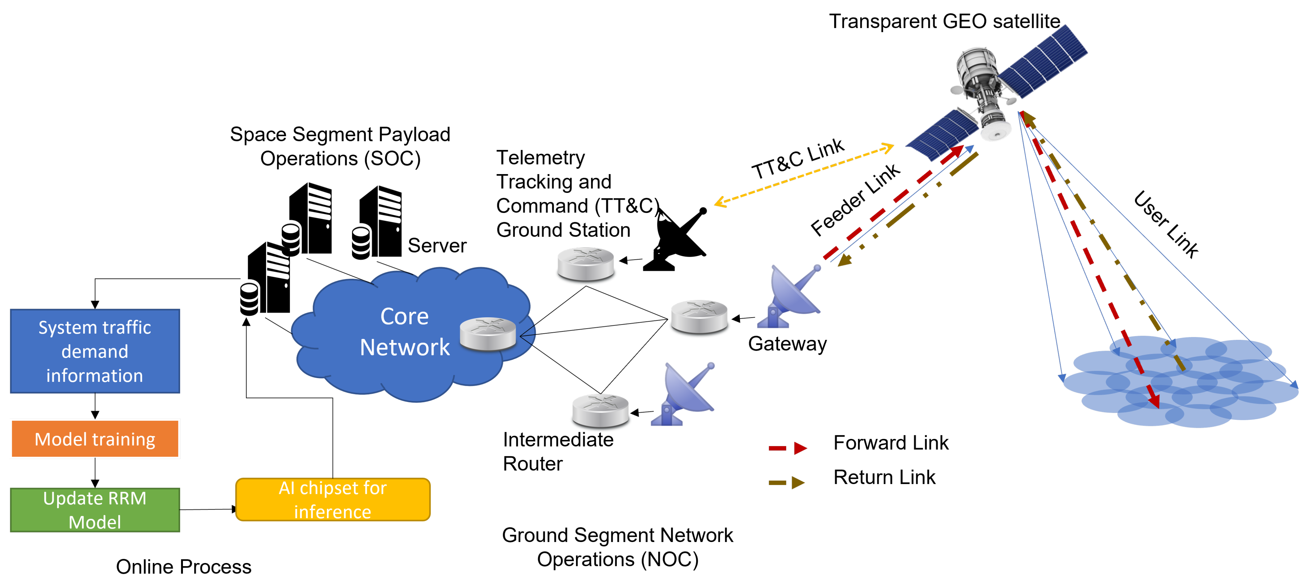
• We define two different system architectures based on ML techniques for RRM depending on whether the AI Chipset is at the ground station or onboard the satellite depending on the training–learning characteristics.
• We study and compare the proposed ML techniques to evaluate their performance and feasibility for both systems.
• We evaluate the performance and processing time required depending on whether training is online or offline.
• We identify the main trade-offs for selecting the commercial AI Chipset that could be used for ML implementation in SatCom systems with a flexible payload.
• We identify different critical challenges for implementing ML techniques for the new lines of research needed.

The remainder of the paper includes the dynamic radio resource management problem and system model in multibeam satellite systems, which is presented in Section 2. Section 3 offers the ML approach for SatCom RRM, discussing the possible architectures and techniques and restructuring the RRM problem to a supervised learning (SL) and reinforcement learning (RL) approach. Section 4 reviews the performance of each system, presenting a tradeoff in the performance of the different models. Section 5 presents discussions on the advantages and disadvantages of the models and architectures presented, the main trade-offs for selecting the commercial AI Chipset and includes open challenges. Finally the conclusions are provided in Section 6.

2. Radio Resource Management

In this section, we describe the RRM problem by considering two different system scenarios: one with flexibility in power, bandwidth and beamwidth and the other with flexibility in illumination time assuming a system with Beam Hopping.

2.1. Power, Beamwidth and Bandwidth Flexibility

We assume a GEO high-throughput satellite system cp, comprising a single GEO multi-beam satellite providing coverage to a wide region of Earth via B spot-beams. We focus on the forward link and assume a total number of K single-antenna User Terminals (UTs) distributed across the overall satellite coverage area. We assume that the considered payload can flexibly manage three resource settings, i.e., power, bandwidth and beamwidth, similarly to [37,38]. From a practical perspective, the flexible power allocation can be obtained by using a TWTA (Traveling Wave Tube Amplifiers) by adapting IBO (Input Back-off). At the same time, the flexible payload must be able to separate the signals into frequency blocks and then reorder them to obtain a flexible bandwidth. This process requires a channelizer onboard the satellite, as mentioned by the authors in [39], to identify the frequency plan (color assignment by frequency and polarization). Finally, to achieve beamwidth flexibility, the OMUX (Output Multiplexer) of the traditional payload should be replaced by reconfigurable BFNs (Beamforming Networks). The change of BFN configuration is halfway between the possibility of synthesizing any beam and choosing from a set of configurations for the same coverage [40].

The heterogeneous traffic demand distribution over the satellite beams and the variations of such traffic demand during the satellite lifetime are the main motivations behind the recent emergence of dynamic radio resource management [8]. In order to adapt to actual demands, the proposed system manages radio resources. The payload manager receives input data from gateways and user beams and then generates optimal control by using the ML model to reconfigure the satellite. The goal of RRM is to manage the available resources to minimize the error between the offered capacity ($C_t^b$) and the requested capacity ($R_t^b$) in bth beam at time slot t.

It may seem feasible to achieve a solution using optimization techniques at a larger scale. However, the number of resources to be managed, the constraints coming from the system and the huge number of traffic demand situations may result in a problem that conventional techniques cannot solve. On the other hand, the resource management problem in SatComs is, in most cases, nonlinear and nonconvex due to the logarithmic function as well as the nonlinear dependencies of $CINR$ in the optimization [8]. This is due to the fact that $C_t^b$ can be calculated as $C_t^b=B{W}_t^{bc}S{E}_t^b$, where $S{E}_t^b$ is the spectral eficiency of the modulation and coding scheme of a commercial reference modem used in the bth beam over t [41]. $S{E}_t^b$ depends on $CINR$ in the bth beam and in turn $CINR$ depends on the power, bandwidth and beamwidth allocated to each beam ($P_t^b$, $B{W}_t^{bc}$ and ${\theta }_t^b$, respectively). In this sense, a generic RRM cost function is defined as follows [33]:

$$\underset{P_t^b,B{W}_t^b,{\theta }_t^b}{min}\frac{{\beta }_1}{B}\sum _{b=1}^B|C_t^b-R_t^b|-\frac{{\beta }_2}{B}\sum _{b=1}^B{P}_t^b-\frac{{\beta }_3}{B}\sum _{nc=1}^{N_c}\sum _{bc=1}^{B_c}B{W}_t^{bc}$$

(1)

such that the following is the case.

$$\left\{\begin{array}{cc}{C}_t^b\ge R_t^b\hfill & P_t^b<P_{max,b},{\theta }_t^b>{\theta }_{min,b},B{W}_t^{bc}<B{W}_{max,b}\hfill \\ C_t^b=C_{max,b}\hfill & P_t^b=P_{max,b},{\theta }_t^b={\theta }_{min,b},B{W}_t^{bc}=B{W}_{max,b}\hfill \end{array}\right.$$

(2)

$$\sum _{b=1}^B{P}_t^b\le P_{max,T}$$

(3)

$$\sum _{bc=1}^{B_c}B{W}_t^{bc}\le B{W}_{max,c}$$

(4)

$${\theta }_t^b\in \left\{{\theta }_1,{\theta }_2,...,{\theta }_N\right\}$$

(5)

The cost function aims to minimize three parameters for each time instant, t. The first parameter is the error between the offered capacity ($C_t^b$) and the required capacity ($R_t^b$), where ${\beta }_1$ (in s/bit) is the weight of the error in the cost function. The second parameter minimizes the total power allocated to all beams (${\sum }_{b=1}^B{P}_t^b$, in W), where ${\beta }_2$ (in 1/W) is the total power weight. The third parameter refers to the total bandwidth (${\sum }_{nc=1}^{N_c}{\sum }_{bc=1}^{B_c}B{W}_t^{bc}$, in Hz) allocated to the beams of each color within the frequency plan, where $B_c$ is the number of beams with the same frequency and polarization defined by color c, $N_c$ is the number of colors in the frequency plan and ${\beta }_3$ (in 1/Hz or s) is the weight of the total bandwidth allocated in each color of the frequency plan.

The cost function constraints are presented in (2)–(5). We show the minimum capacity constraint in (2) where $C_t^b\ge R_t^b$ for each beam, provided if the power and bandwidth assigned to the b-th beam at time t are less than the maximum allowed for each beam ($P_{max,b}$ and $B{W}_{max,b}$ respectively) and the beamwidth is greater than the minimum allowed (${\theta }_{min,b}$). In case the offered capacity cannot satisfy the beam requirement constraint, the offered capacity in the b-th beam will be the maximum possible value.

In addition, the total power allocated to each beam should not be greater than the maximum total power of the system ($P_{max,T}$) (3), and the total bandwidth allocated in each color of the frequency plan should not be greater than the bandwidth per color ($B_{max,c}$) (4). Moreover, the beamwidth of the b-th beam must belong to the set of possible configurations previously established (5), where N represents the size of the set. The beamwidths must also meet the requirement of completely covering the entire service area.

2.2. Beam Hopping

Time flexibility is an alternative scheme where the full available spectrum can be allocated to a subset of the overall spot beams, which are activated only for a specific portion of time. The set of illuminated beams can be changed over time slots according to a periodically repeating spatio-temporal transmission pattern. Co-channel interference is kept to a minimum, keeping the beams belonging to the same group with a minimum geographical separation. The main design problem of a BH system is to identify the optimal illumination pattern of the beams, i.e., which beams are activated when and for how long [30].

The beam scheduling or beam illumination pattern formulation considers a specific time window $T_w$ segmented into time slots of duration $T_s$. In this case, we use “snapshot” to refer to a particular arrangement of illuminated and unilluminated beams. Within a BH window $T_w$, a number of illuminated snapshots are are used. Denote $\mathcal{G}$ as the set of $\mathcal{G}$ possible snapshots and ${\mathcal{G}}_b\subset \mathcal{G}$ as a set of snapshots with illuminated beam b. In that sense, a beam illumination design can be formulated as a $maxmin$ problem where the objective is to maximize the minimum value of the ratio between offered capacity and traffic demand in the entire set of illuminated beams, and $maxmin$ is generally widely used for fairness purposes, such as fairness in satisfying user demand [8]:

$$\underset{t_g}{max}\underset{b}{min}\left\{\frac{C_g^b\frac{{\sum }_{g\in {\mathcal{G}}_b}{t}_g{T}_S}{T_W}}{D_g^b}\right\}$$

(6)

such that the following is the case:

$$\sum _{g=1}^{\mathcal{G}}{t}_g{T}_s=T_w$$

(7)

$$\{t_1,t_2,...T_{\mathcal{G}}\}\in \mathbb{I},$$

(8)

where $C_g^b$ represents the offered capacity, $D_g^b$ represents the traffic demand on the bth beam and $t_g$ is the normalized illumination time for the gth snapshot.

Based on its features, (6) is a mixed integer linear programming (MILP) problem. To simplify the proposed problem, a reformulation is usually carried out that relaxes the integers to non-negative continuous numbers. Then, the objective function is transformed from a max–min to maximization-only by introducing an auxiliary variable as explained in [30]. However, the illumination time per beam must be provided as a function of traffic demand, as well as taking into account the number of simultaneously active beams and user latency as explained in [8]. Therefore, an ML-assisted model is expected to help improve the optimization performance presented in Equation (6) without having to resort to the aforementioned simplifications.

3. ML for SatCom RRM: Architecture and Techniques

3.1. Machine Learning Implementation in SatComs Systems

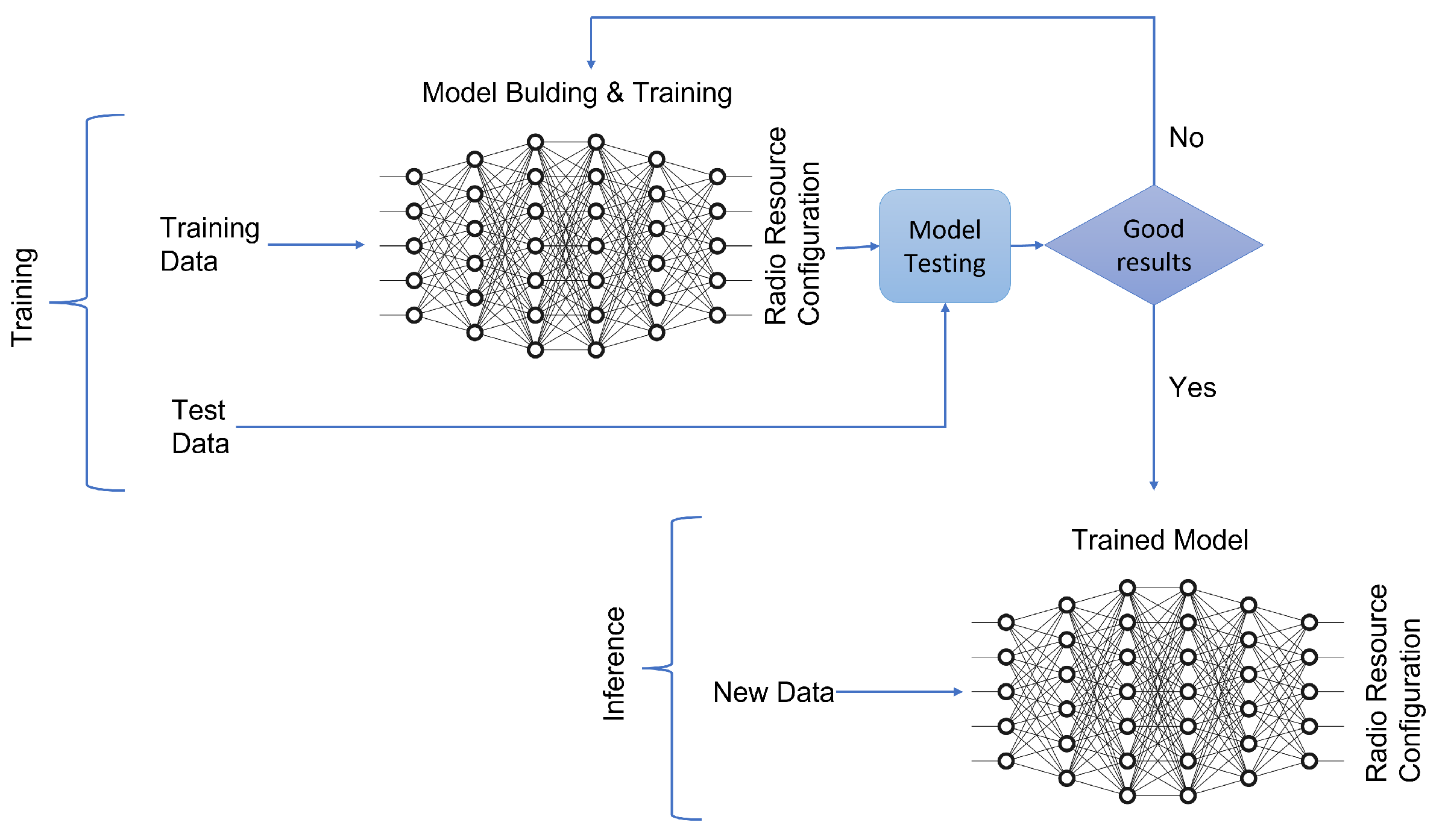
3.1.1. Online or Offline Learning

ML techniques for RRM undergo two phases, as shown in Figure 1: training and inference. Initially, the ML model experiences the training stage. The objective is to find the optimal model parameters to predict the radio resource configuration at the satellite for the system conditions. Then, the trained model is obtained and used to indicate the best payload resource allocation.

In this regard, one of the first decisions to make when implementing ML for RRM is whether learning should be online or offline. Online learning means learning as the data comes in. Offline means that a static dataset is available. Thus, with online learning, more data are (usually) available, but there are time constraints.

A system trade-off exists between the type of training selected. Depending on the service requirements, one option can be chosen. Suppose the most important objective is to maintain the quality of service and availability. In that case, online training can be chosen as it has the ability to better adapt to sudden and abrupt changes in the system over time because learning is constantly updated. However, it requires processing times to be invested in the training, which can delay updating the resources in the payload.

On the other hand, if offline training is chosen, processing times are reduced since inference on a trained ML model requires a low computational cost compared to the training phase. The ML model acts as an intelligent switch that selects the payload resource configuration based on the current system requirements. Nevertheless, a large database may be required to obtain a successful training that considers multiple RRM parameters, and the model may present large errors for unexpected situations in the system.

This presented trade-off has a strong impact on the implementation of the AI Chipset in the system as explained in Section 3.1.2.

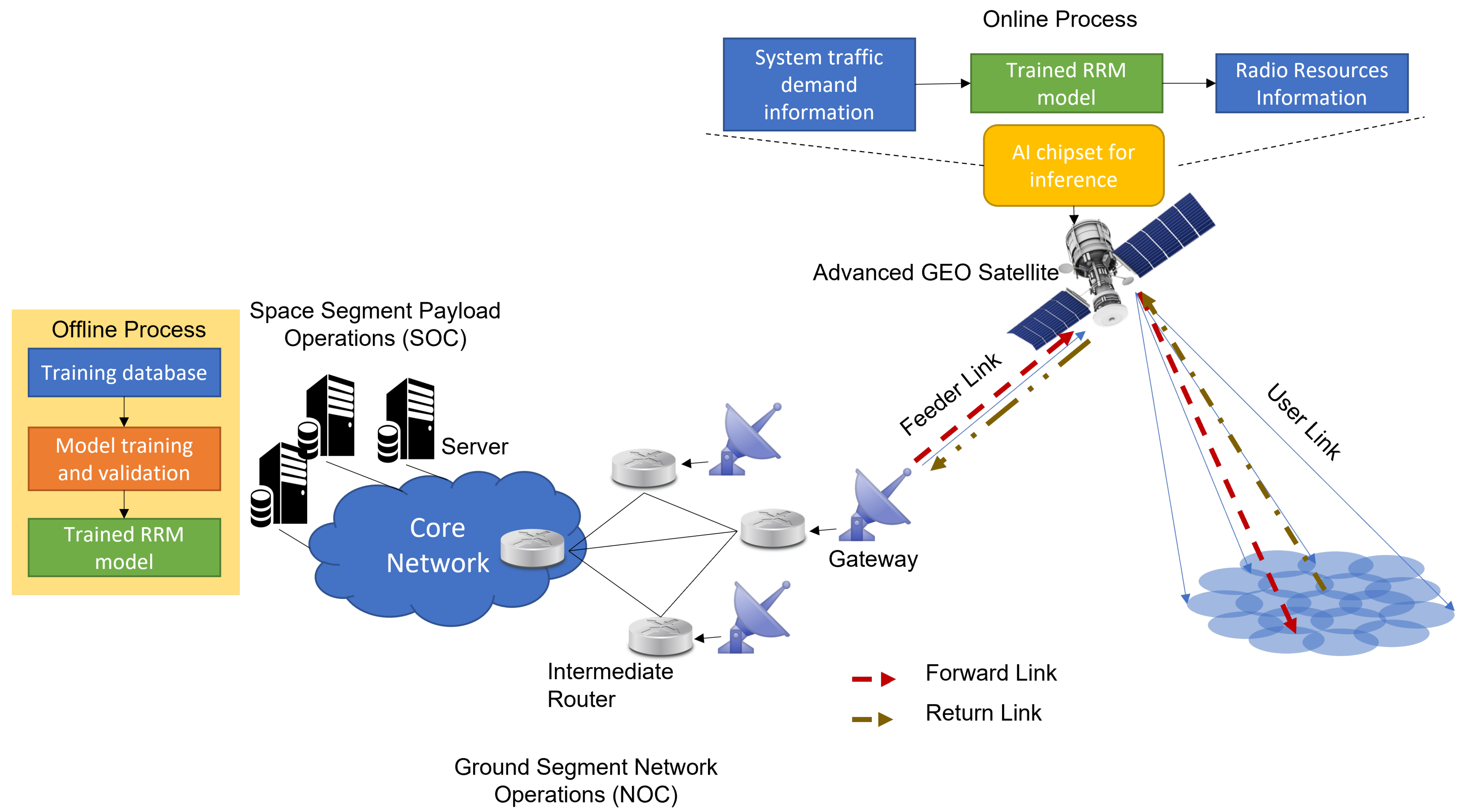
3.1.2. Ai Chipset On-Ground or On-Board

Selecting the most suitable system architecture to meet the minimum service requirements is one of the main challenges of implementing ML techniques in SatComs systems. In this sense, in Figure 2 and Figure 3, we propose two system architectures that use ML techniques to automate the RRM process. The main difference resides in whether the AI Chipset is onboard or on-ground.

The first proposed architecture (Figure 2) represents process automation implementation using an ML algorithm trained online. For this scenario, the AI Chipset is part of the ground segment because the trained model must be updated every time. Information on the system traffic demand, on the geographical distribution of users and on channel information is obtained through the return link, which will reach the servers connected to the system gateway network. The data are processed to train the ML model with which the RRM policy is updated, and the AI Chipset is used for inference. The information on how the radio resources should be distributed on the satellite is generated. By using TT&C (Telemetry, Tracking and Command), this information is transmitted to the satellite, allowing the satellite to manage the radio resources for the user link.

The main advantage of this architecture (Figure 2) is that the system will have greater flexibility to adapt to unforeseen changes, e.g., a drastic and unexpected change in traffic demand. Thus, obtaining an outstanding performance in the automation of the RRM process since the updated RRM model is obtained with the instantaneous values of the actual system. However, there are two main disadvantages: (i) the processing time due to which could add a delay in updating the satellite radio resources and (ii) the signaling and reallocation of resources may introduce performance degradation to the system.

On the other hand, the second proposed architecture (Figure 3) is based on training the offline ML model with a training database that describes the system behavior. A model that manages satellite resources according to user link conditions could be obtained. Once the model has been trained, the AI Chipset could be located onboard the satellite [35] for inference. The main advantage of this architecture (Figure 3) is that processing times are reduced, firstly because the model has been previously trained. However, a return channel demodulator would be required to analyze the traffic demand in real-time or an additional ML block for onboard traffic prediction is also feasible; thus, this architecture has a strong dependency on the training data and the models used. This will imply additional complexity and power needs onboard. In addition, the dependence of the traffic model could affect the performance of the RRM in case of drastic changes in the actual system and the training has to be redone; furthermore, the cost and mass of the payload would be increased.

A third scenario would be a hybrid architecture where model training is initially performed online. However, it is possible to update the trained model by collecting new data obtained during the forward link.

3.2. Supervised Learning for RRM

SL is a technique for deducing a function from training data. The training data consist of pairs of objects: One component of the couple is the input data, and the other is the desired results. The function’s output can be a numerical value (as in regression problems) or a class label (as in classification problems). Supervised Learning aims to create a function capable of predicting the value corresponding to any valid input object after having observed a set of examples: the training data. To perform this, one must generalize from the presented data to previously unknown situations [42].

On the other hand, neural networks (NN) are a model inspired by the behavior of the human brain. It consists of a set of nodes known as artificial neurons that transmit signals to each other. These signals are transmitted from input to output. The NN consists of three different layers: (i) the input layer, where the input variables that can represent the characteristics of the system are located; (ii) the output layer, where the output variables are located and represent the information acquired from the input variables; (iii) and the hidden layers, where information is propagated and analyzed to obtain an expected output. NN training is performed through backpropagation, which consists of propagating the error between the desired and expected output from the last layer to the first, modifying the weights of the neural connections until the error is minimized [43].

In that sense, NNs represent a viable option to optimize and automate the RRM in a multibeam SatComs system. We will focus specifically on approaching the problem using Deep Neural Networks (DNN) [30,31] and Convolutional Neural Networks (CNN) [33].

When the system is offline, training data are generated first, and labels are assigned to training data to minimize the RRM cost function. NN training is performed offline, and resource management responds to the traffic demand using supervised learning.

In other words, NN represents only an intelligent switch for the payload that changes from one configuration to another whenever the system requirements change; the change is made instantaneously, i.e., the impact of a delay in updating resources on capacity is negligible. NN performance during training is crucial, and it is also important to avoid overfitting, as this will depend on resource management.

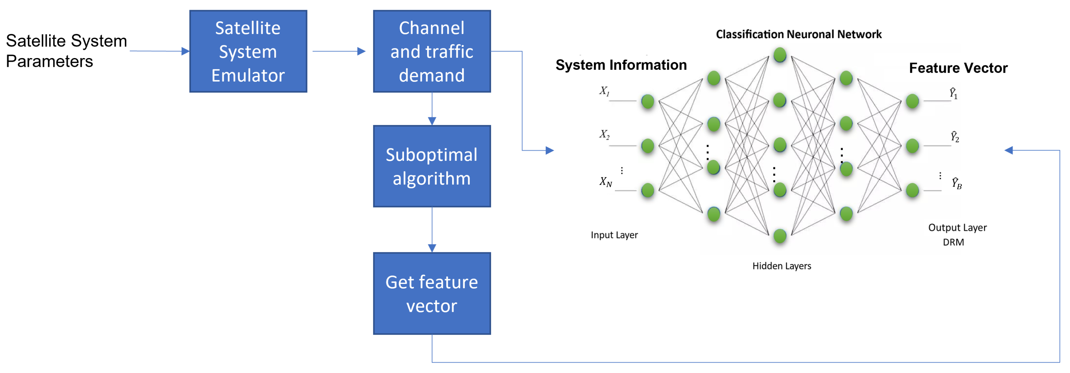
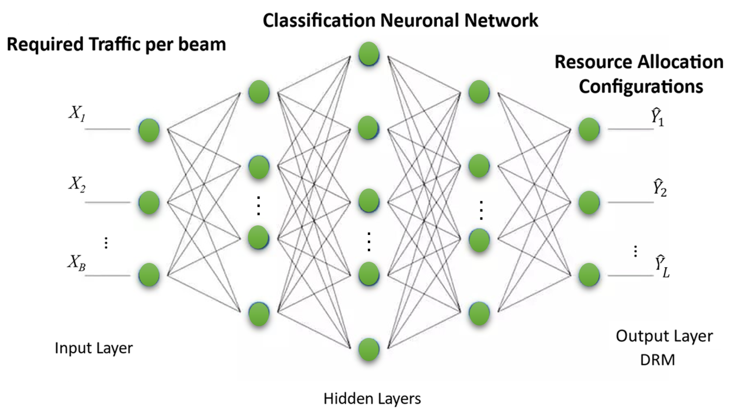
3.2.1. Dnn-Based RRM: Power, Beamwidth and Bandwidth Flexibility

In this section, we study the DNN architecture for payload resource management onboard a multibeam satellite with B user beams. The system will respond to changes in traffic demand by modifying two radio resources: bandwidth and power for a limited number of beams. A training database is generated with different possible traffic demand values for the beams based in the traffic model explained in [32]. For each of these possible combinations of the required capacity in each beam, there is a label indicating the configuration of the resource allocation set that minimizes the cost function (1) and meets constraints (2)–(5) [31]. The cost function (i.e., the regularized logistic regression) for DNN training can be written as follows:

$$\begin{array}{cc}\hfill J(\widehat{Y},W)& =-\frac{1}{m}\sum _{i=1}^m[Y^{\left(i\right)}·log\widehat{Y}\left(X^{\left(i\right)}\right)+\left(1-Y^{\left(i\right)}\right)log\left(1-\widehat{Y}\left(X^{\left(i\right)}\right)\right)]+\frac{\lambda }{2m}\sum _{j=1}^k{W}_j^2\hfill \end{array}$$

(9)

where m represents the number of training samples, $X^{\left(i\right)}$ indicates the ith training example with possible required capacities in each beam, $X^{\left(i\right)}=[X_1^{\left(i\right)},X_2^{\left(i\right)},...,X_B^{\left(i\right)}]$, $Y^{\left(i\right)}$ denotes the ith configuration corresponding to $X^{\left(i\right)}$, $\widehat{Y}\left(X^{\left(i\right)}\right)$ is the configuration predicted for $X^{\left(i\right)}$, k is the order of logistic regression and $\lambda$ is the regularization parameter to avoid overfitting. Logistic regression optimizes the log loss for all observations in which it is trained, which is equivalent to optimizing the average cross entropy.

In this sense, Figure 4 serves as a reference for understanding how the problem is addressed. The vector $X=[X_1,X_2,\dots ,X_B]$ represents the B (number of beams) inputs of the Neural Network. Vector $\widehat{Y}$ represents the L outputs of the Neural Network, and the L outputs correspond to the set of possible resources allocated to the each of the B beams.

3.2.2. DNN-Assisted RRM: Beam Hopping

On the learning point of view, traditional end-to-end learning approaches can help to provide a suboptimal solution to the cost function proposed in (6). However, it is generally only applicable to limited cases, e.g., a problem with few variables, non-strict or no constraints. It imposes difficulties for training and, therefore, can significantly increase the difficulty in achieving prediction accuracy. In that sense, the author in [30] explored a combined method for BH design to obtain the benefits of optimization and learning.

A classifier is trained using a DNN to identify a small subset of promising snapshots. Promising snapshots means that they are with high probability to appear in the optimal illumination pattern. The feature vector consists of B binary elements corresponding to the number of beams, $Y=[Y_1,...,Y_b,...,Y_B]$, where $Y_b$ represents whether any snapshot with bth active beams is scheduled at the optimum ($Y_b=1$) or none of the snapshots of bth is used ($Y_b=0$).

The training dataset contains two parts: the input parameters and the optimal or suboptimal labels. The data generation procedure is illustrated in Figure 5. The ith training set is denoted as $(X^{\left(i\right)},Y^{\left(i\right)})$. The input $X^{\left(i\right)}$ is obtained by the ith realization in emulators, which consists of the channel matrix H, the traffic demand per beam $[D_g^1,...,D_g^B]$ and the power per beam $[P_g^1,...,P_g^B]$ in gth snapshot, where an adopted satellite emulator generates the beam coverage area and H. The DNN accepts only real-valued inputs; thus, the original complex value in H is converted to real values. The labels are organized as feature vector $Y^{\left(i\right)}$ for the ith realization. The DNN is trained to learn the mapping of the input to the optimal label. After being trained, the model can provide an efficiently predicted feature vector that can be used in conjunction with a conventional optimization algorithm.

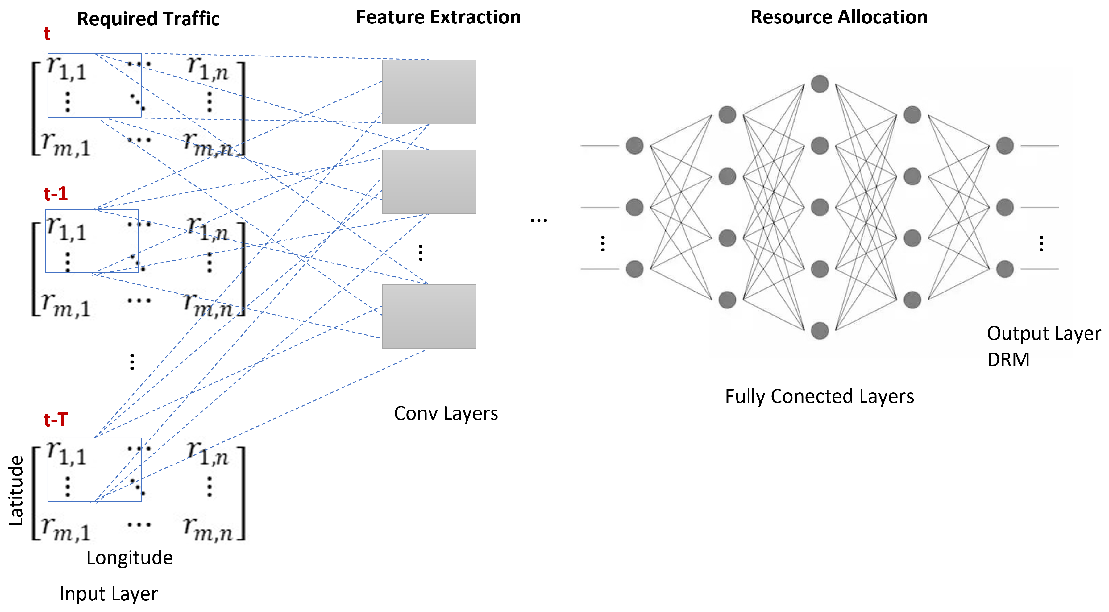
3.2.3. Cnn-Based RRM: Power and Bandwidth Flexible

A CNN architecture, generally considered in image classification problems [44], is proposed to adapt it to solve the RRM problem, in this case for power, bandwidth and beamwidth management [33]. The adaptation of the traditional CNN architecture is performed at the input layer and the output layer. At the input layer of the CNN, there is a matrix tensor, and each matrix represents the traffic demand at each geographic location in the service area. The service area does not have a regular geometric shape; thus, the geographic coordinates contained in each matrix outside the service area are zero-filled. In this proposed work, the matrix tensor does not represent the channels of an image but the time instants (states) at which the system is evaluated. That is, the depth of the matrix tensor is given by vector $\{t,t-1,t-1,t-2,...,t-T\}$, where t is the current time instant, and T is the size of the time window and represents the size of the observed states for RRM.

Depending on features extracted by the convolutional layers, the constraints and the payload flexibility, there is a set of possible configurations for the resource allocation in beams. These possible configurations are encoded in a vector of size L, representing the number of possible configurations of the payload resources. Taking advantage of this, the CNN has at the output layer the configuration that minimizes the cost function in (1) for the input layer conditions.

A schematic of the different layers of the CNN is shown in Figure 6. A matrix tensor starting with the traffic demand at each geographic coordinate is the input layer. Then, the convolution layers are used to obtain the main features of the traffic demand at the geographic coordinates. Full connection layers are used to map the resource configuration with the features obtained in the convolution layers. The output layer results in a resource allocation that minimizes RRM cost function (1). In the convolutional layers, the features are extracted from the kernels obtained at the output $Y_j$, as represented in the following:

$$Y_j=f_1(p_j+\sum _i{K}_{ij}\otimes Y_i)$$

(10)

where $Y_j$ represents the output of the jth neuron and is a matrix computed as the linear combination of the outputs $Y_i$ of the neurons in the previous layer. Each operated on with the convolutional kernel $K_{ij}$ corresponding to that connection; this quantity is added to a connection $p_j$ and then passed through a nonlinear activation function $f_1(·)$. The convolution operator has the effect of filtering the input matrix with a previously trained kernel.

The CNN that manages resource allocation is the core of the RRM. The CNN determines how to match resources to a demand pattern while minimizing payload resource consumption. Network training is performed offline; thus, the CNN represents an intelligent switch that functions as DRM for the satellite communication system.

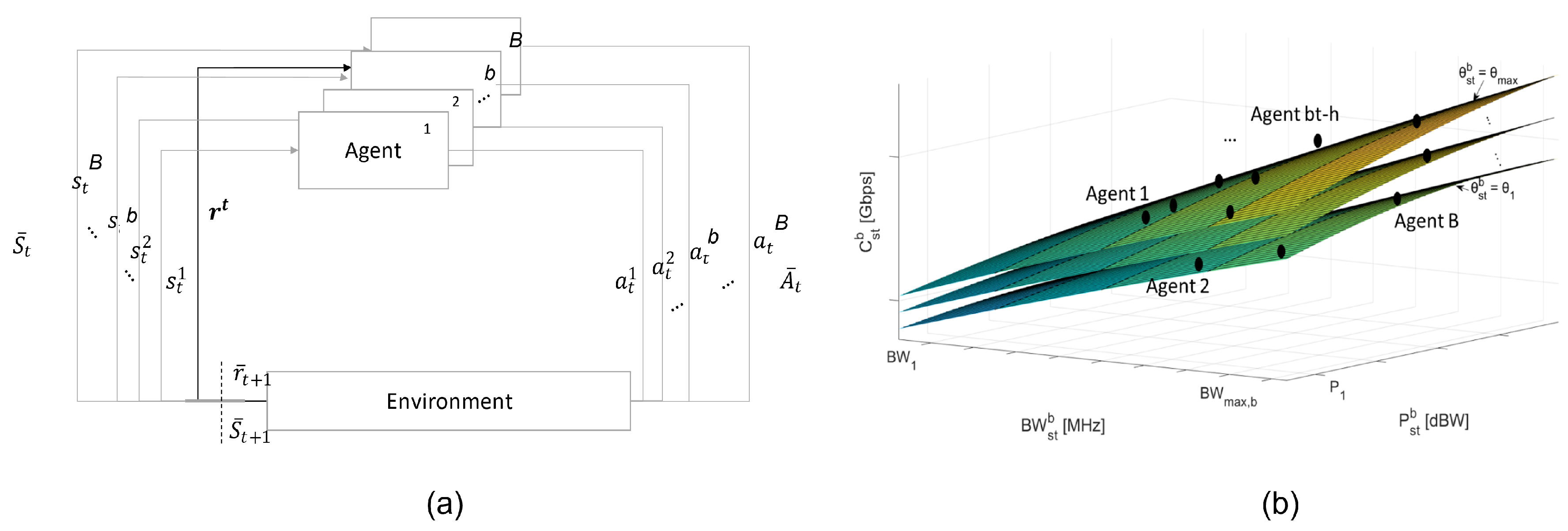
3.3. Reinforcement Learning for RRM

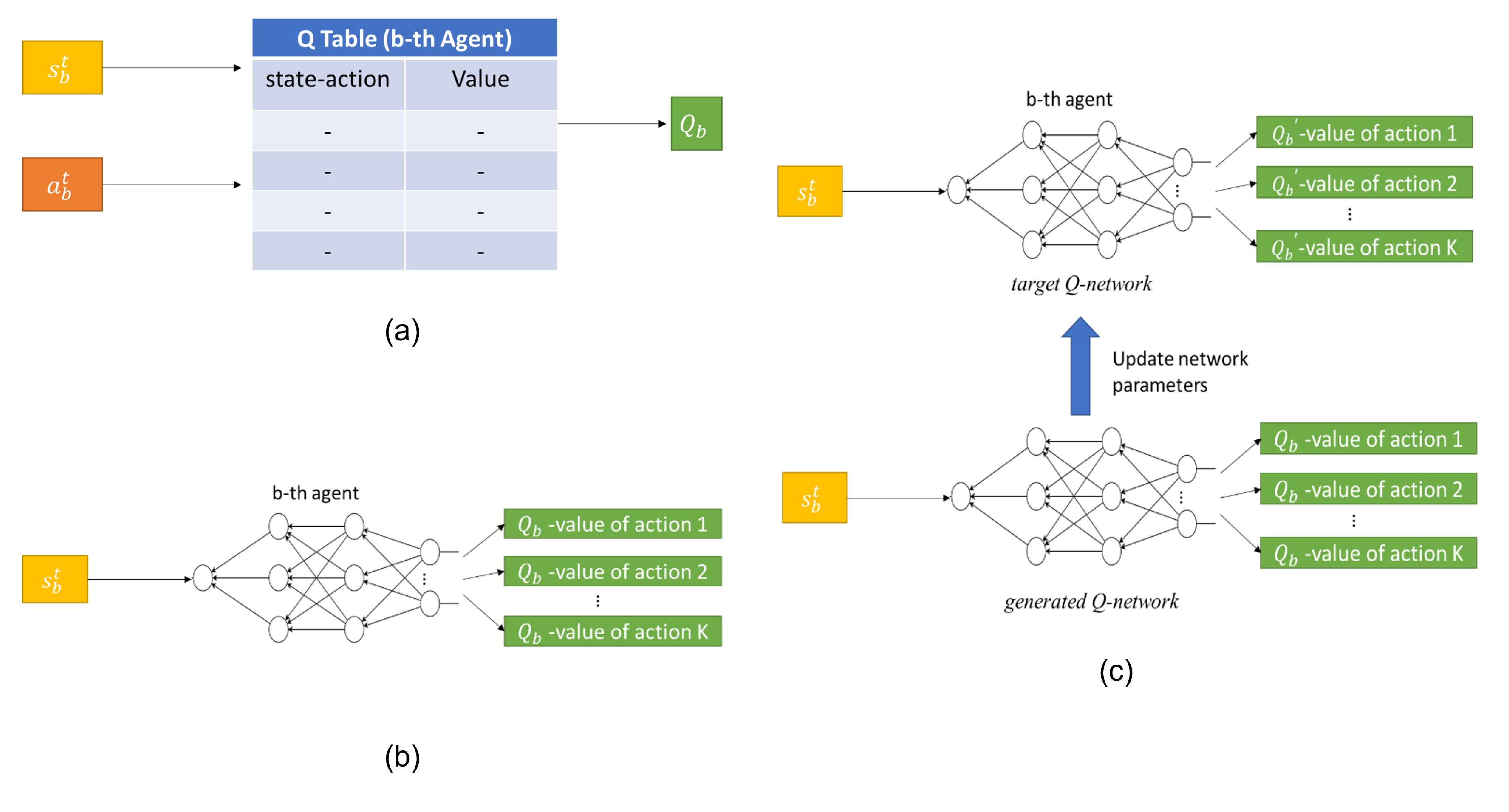
Reinforcement learning is an area of ML focused on identifying actions that must be performed to maximize the reward signal; in other words, it is concerned with mapping situations to actions focused on seeking that reward. The agent in RL represents the hardware or software that must learn to perform a specific action; in that sense, the agent interacts with an “environment”, which may be an actual decision process or a simulation. The agent works by observing the environment and making a decision and checking what effects it produces. Suppose that the result of that decision is beneficial. In that case, the agent automatically learns to repeat that decision in the future, while if the effect is detrimental, it will avoid making the same decision again [45].

The Markov Decision Process (MDP), on the other hand, provides a mathematical framework on how to model the interaction between the agent and the environment. A stochastic discrete-time model for which its evolution can be controlled over time is the key objective of MDP. The control policy is associated with a stochastic process and a value function. Our goal is to find the “best” policy that solves the described problem. MDP contains a set of states $s\in S$, a set of actions $a\in A$, a reward function $r\in R$, and a set of transition probabilities $p\left(s_{t+1}\right|s_t,a_t)$ to move from the current state $s_t$ to the next state $s_{t+1}$ given an action $a_t$. The objective of an MDP is to find a policy that maximizes the expected cumulative rewards $R={\sum }_{i=0}^{\infty }{\gamma }^i{r}_{t+i}$, where $r_{t+i}$ is the immediate reward at time $t+i$, and $\gamma \in [0,1]$ is the discount factor.

According to the current state-of-the-art, reinforcement learning algorithms have been proposed to manage the resources of a multibeam satellite, even though it is still at an infancy stage. However, these algorithms can only manage a single resource in a multibeam system [27]. Regardless, a fully flexible payload must manage at least three resources (i.e., power, bandwidth and beamwidth). In that sense, we assume that as the available resources to operate across all satellite beams increase, it becomes a very challenging problem for a single agent (SA). Therefore, we proposed a Cooperative Multi-Agent (CMA) approach with better performance than SA [34].

The proposed system manages communication resources in response to changes in traffic demand. Resource management training is assumed to be performed online, i.e., whenever traffic requirements change, and the values are updated to retrain the RRM agents given the new conditions. For this reason, the processing time will play a critical role in the performance of RRM that must manage the available resources to minimize the error between the capacity offered at each beam and the required traffic demand and, at the same time, optimize the resources used over time.

The RRM cost function can be reformulated as a multi-agent MDP that works cooperatively to achieve the maximum reward, as seen in Figure 7. All agents share the same reward, but each agent must meet some minimum conditions, which guarantees that, despite working cooperatively, each agent will seek its benefit. In the proposed cooperative environment, there is a global reward function, and each agent will know the states and actions of all agents. Each agent must meet the minimum requirements to achieve equilibrium in the system. The illustration of the CMA is shown in Figure 7a. Considering a multi-agent environment involving B agents, the bth agent observes the state of the globally shared environment and independently selects an action to perform. Then, the current state is transformed into a new state. All agents are in the same environment and have a common goal; thus, they work in cooperation to maximize the reward where ${\overline{S}}_t=\{s_t^1,s_t^2,\dots ,s_t^B\}$ represents the current states of the agents, and ${\overline{A}}_t=\{a_t^1,a_t^2,\dots ,a_t^B\}$ represents the actions.

In MDP, $C_{s_t}^b$ is the capacity offered in the bth beam in the current state, $D_{s_t}^b$ is the traffic demand, $P_{s_t}^b$ represents the allocated power, $B{W}_{s_t}^b$ means the allocated bandwidth, and ${\theta }_{s_t}^b$ represents the allocated beamwidth in the bth beam in the current state. In this sense, $C_{s_t}^b\in \{C_1,C_2,...,C_{max,b}\}$ is calculated assuming that $P_{s_t}^b\in \{P_1,P_2,...,P_{max,b}\}$, $B{W}_{s_t}^b\in \{B{W}_1,B{W}_1,B{W}_2,...,B{W}_{max,b}\}$ and ${\theta }_{s_t}^b\in \{{\theta }_1,{\theta }_2,...,{\theta }_{max}\}$. The space of all capacity values that can be assigned to the bth beam depends on the resources assigned to the bth beam (Figure 7b). In this sense, by maintaining a given beamwidth, the bth agent can move north, south, east or west as long as it is within the limits of the resource allocation space. The movement of the agent corresponds to a new power or bandwidth allocation. Each surface represents a beamwidth value. The bth agent can jump from one surface to another (jump up or jump down) as long as it is within the boundaries of the resource allocation space. This jump corresponds to a new beamwidth allocation.

Information about the convergence time of the algorithm is essential for the RRM system since training is online. Based on this, three different RL algorithms were proposed (Figure 8), i.e., Q-Learning (QL), Deep Q-Learning (DQL) and Double Deep Q-Learning (DDQL). The RRM first observes the current environment, represented by the traffic demand and the offered capacity based on the resource allocation. The agents are trained from the acquired observation data using an RL algorithm to obtain the agents’ policies and tp update the resources. This is repeated each time the traffic demand changes. The goal of RL is to extract which actions should be chosen in different states to maximize the reward. In a sense, B agents are sought to learn a policy, which we can formally view as an application that tells each agent what action to take based on its current state. The agents’ policy is divided into two components: on the one hand, how each agent believes that an action refers to a given state and, on the other hand, how the agent uses what it knows to choose one of the possible actions.

3.3.1. Q Learning

In the QL algorithm, the $Q_b$ value of a pair $(s_t^b,a_t^b)$ contains the sum of all possible rewards for each state-action of the bth agent at instant t. Provided that the bth agent knows a priori the $Q_b$ values of all possible pairs $(s_t^b,a_t^b)$, it could use this information to select the appropriate action for each state. Table Q is generated for each agent (Figure 8a), representing a matrix of size $J\times K$ where J is the number of possible states of the bth agent and K the number of possible actions, and in each position of the matrix, the $Q_b$ value for each state-action pair is represented. The first objective of the agent is to approximate as much as possible the assignment of $Q_b$ values, which depends on both future and current rewards, as shown in the following:

$$Q_b(s_t^b,a_t^b)=r_t(s_t^b,a_t^b)+\gamma [\underset{a_t^b}{max}{Q}_b(s_{t+1}^b,a_t^b)]$$

(11)

where $s_{t+1}^b$ represents the following state, and $\gamma$ is the discount factor controlling future rewards’ contribution. Since this is a recursive equation, it starts by making arbitrary assumptions for all $Q_b$ values and is implemented as an update:

$$\begin{array}{cc}\hfill Q_b(s_t^b,a_t^b)& \leftarrow Q_b(s_t^b,a_t^b)+\alpha [r_t(s_t^b,a_t^b)+\gamma \underset{a_t^b}{max}{Q}_b{(s_{(}t+1)}^b,a_t^b)-Q_b(s_t^b,a_t^b)]\hfill \end{array}$$

(12)

where $\alpha$ is the learning rate or step size; this determines the extent to which newly acquired information overrides old information.

3.3.2. Deep Q Learning

DQL uses a neural network to approximate the function of the $Q_b$ value, thus avoiding the use of a table to represent it (Figure 8b). At the input of the neural network, there will be the state of the bth agent, and at the output, there will be the $Q_b$ for each of the possible actions; the bth memory, $M_b$, stores all the experiences. The loss function of the neural network is the mean square error of the predicted $Q_b$ value and the target $Q_b^{\prime }$ value:

$$L_b(s_t^b,a_t^b,{\omega }_t)={(Q_b^{\prime }-Q_b(s_t^b,a_t^b,{\omega }_t))}^2$$

(13)

$$Q_b^{\prime }=r_t(s_t^b,a_t^b,{\omega }_{t-1})+\gamma \underset{a_t^b}{max}{Q}_b^{\prime }(s_{t+1}^b,a_t^b,{\omega }_{t-1})$$

(14)

where $Q_b^{\prime }$ is the temporal difference target, and $Q_b^{\prime }-Q_b$ is the temporal difference error; ${\omega }_t$ is the current neural network parameters and ${\omega }_{t-1}$ includes the previous parameters.

3.3.3. Double Deep Q Learning

Each agent in DDQL uses two neural networks with the same architecture to learn and predict what action to perform at each step (Figure 8c). A DDQL model includes two deep learning networks, called generated Q-network $\left(Q_b(s_t^b,a_t^b,{\omega }_t)\right)$ and target Q-network $\left(Q_b(s_t^b,a_t^b,{\omega }_t^{-})\right)$, where ${\omega }_t^{-}$ includes the parameters of the current target neural network.

DDQN can produce more accurate value estimates and leads to better overall deep neural network performance. The generated Q-network is used to generate actions, and the target Q-network is used to train from randomly selected observations from the replay memory. The replica memory of the DDQN stores the state transitions received from the environment, allowing the reuse of these data. By randomly sampling it, the changes forming a batch are related to the decorrelation, stabilizing DDQN. The generated Q-network is used to calculate the bth value $Q_b$ for the bth agent. At the same time, the target Q-network aims to produce the target $Q_b^{\prime }$ value to train the parameters of the generated Q-network. According to the basic idea of DDQL, the target value $Q_b^{\prime }$ can be defined as follows.

$$Q_b^{\prime }=r_t(s_t^b,a_t^b,{\omega }_{t-1})+\gamma Q_b(s_{t+1}^b,arg\underset{a_t^b}{max}{Q}_b(s_{t+1}^b,a_t^b,{\gamma }_{t-1}),{\omega }_t^{-})$$

(15)

4. Performance Evaluation

In this section, we present the performance evaluation of different approaches of ML techniques for RRM on GEO multibeam satellites. The satellite environment and traffic demand were simulated using MATLAB R2020a based on the traffic model presented in [33]. The software toolchain used to implement the ML models consists of a Python development environment called Jupyter involving Keras 2.0. It is essential to mention that the running time obtained directly depends on the computer features used for the training, which for this paper was an Intel (R) Core (TM) i7-7700HQ 2.8 GHz CPU and 16 GB RAM.

4.1. Simulation Parameters

A GEO multibeam satellite with flexibility in frequency, bandwidth and beamwidth and with a four-color frequency plan scheme to avoid co-channel interference is assumed for the analysis. We evaluate the performance of different ML models by numerical simulations.

In that sense, the

Table 3. Features of the ML models evaluated.

ML Technique	Model	Training	Implementation
Supervised Learning	DNN	offline	On-board
	CNN
Reinforcement Learning	QL	online	On-ground
	DQL
	DDQL

shows the main features of different ML models that have been evaluated for RRM on GEO multibeam satellite. It is noted that the models based on supervised learning are assumed to be trained offline; therefore, the AI Chipset could be onboard the satellite operating only as an intelligent switch that adapts the resources according to the traffic demand. On the other hand, for the reinforcement learning based models it is assumed that the training will be online, i.e., the model will be trained every time the traffic requirements change drastically so the AI Chipset will be on ground and, by using TT&C, it will send the information to the satellite to update the resources (see Section 3.1). The architecture used for each ML model can be found in the Appendix A.

In addition,

Table 4. System parameters.

Parameter	Value
Satellite Orbit	9° E
Number of Beams	82
Noise power density	−204 dBW/MHz
Max. beam gai	51.8 dBi
User antenna gai	39.8 dBi
Maximum bandwidth per beam	500 MHz
Maximum power per beam	100 W
Total available transmit power	1000 W

provides a summary of the main simulation parameters. The traffic model used is based on the model presented in [34], which represents a service area similar to that of the KaSat satellite [46] with 82 beams. The flexible parameters per beam are power with 8 to 17 dBW with 0.1 dB steps, bandwidth with 100, 150, 200, 250, 250, 300, 350, 350, 400, 450 or 500 MHz and beamwidth with 0.55, 0.60 or 0.65 degrees.

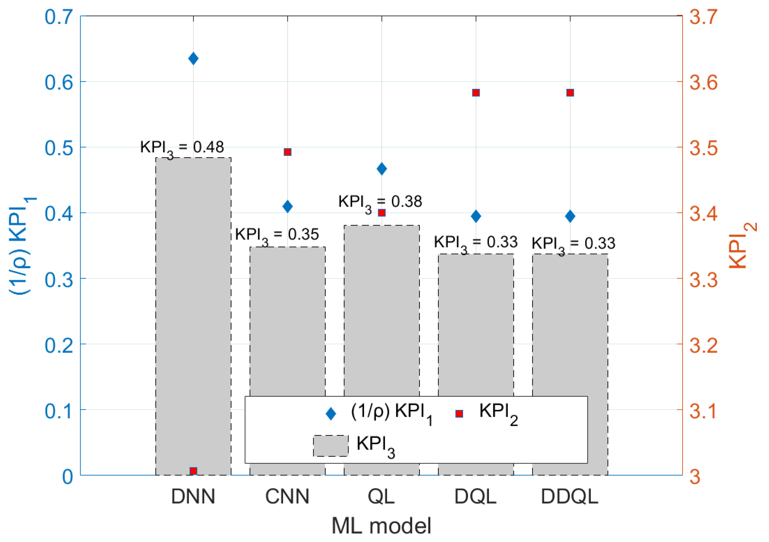
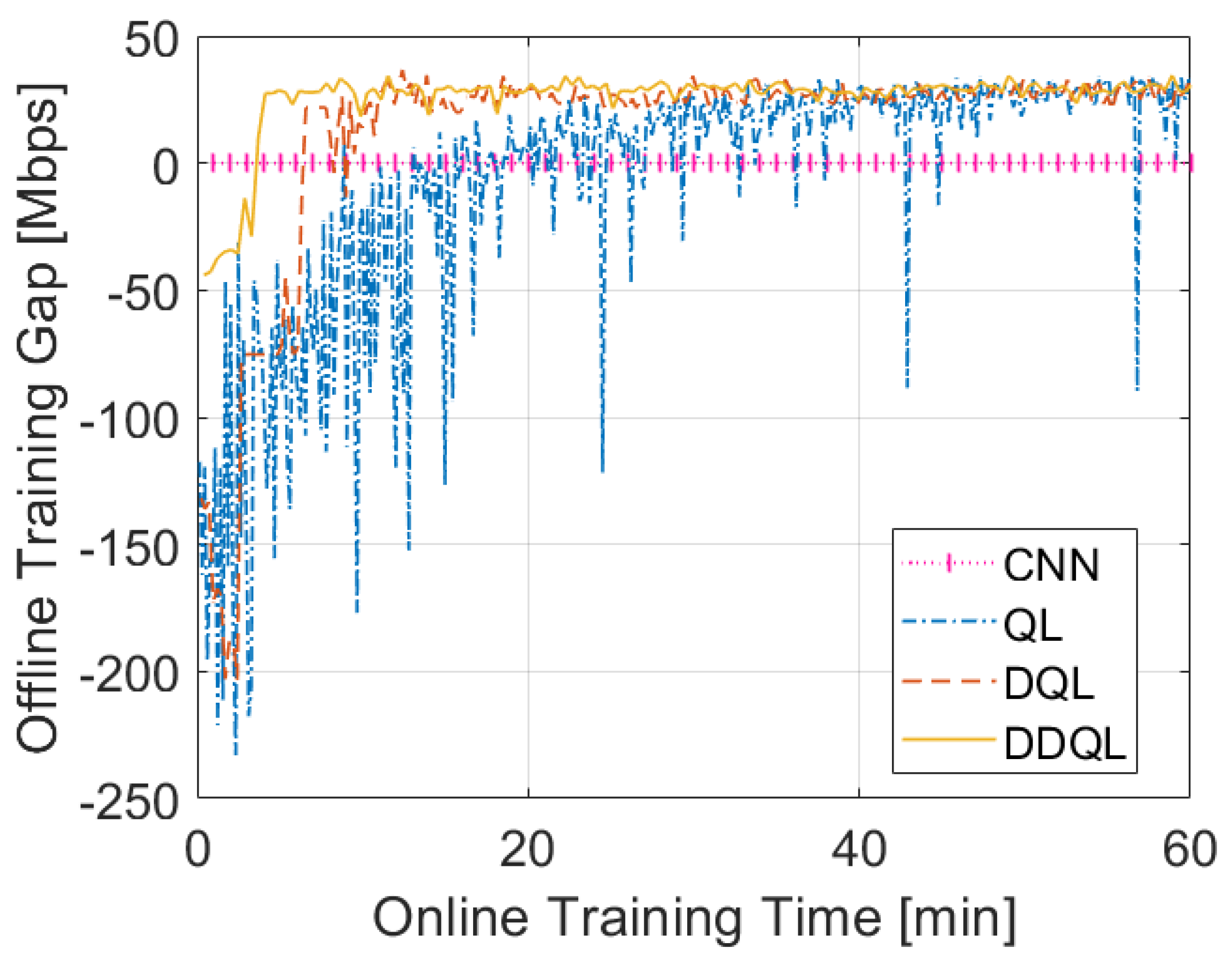
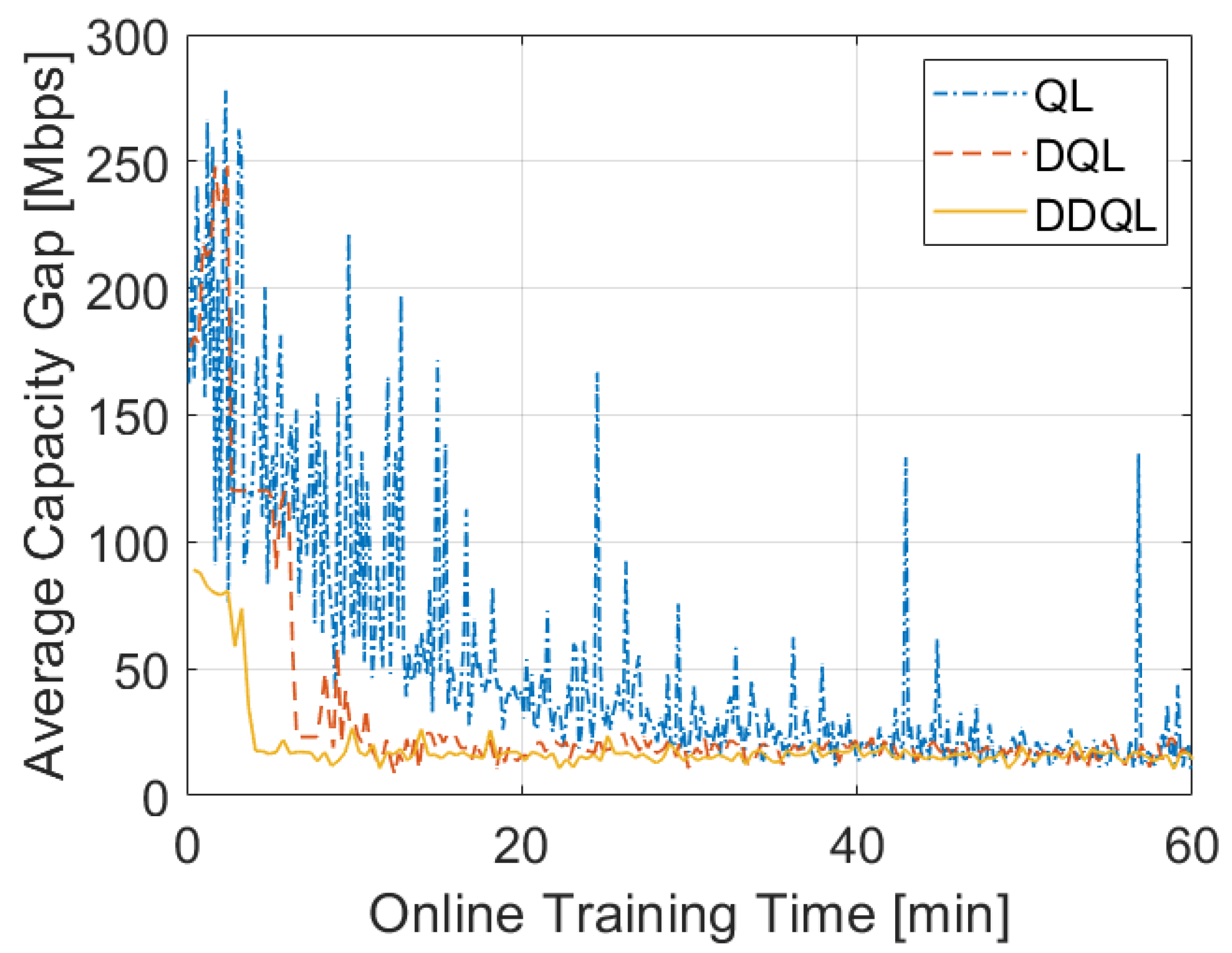
4.2. Performance Comparison

Cost function adopted for the optimization is Equation (1), which aims to minimize the difference between the traffic demand and the offered capacity and at the same time to minimize the resources used in the satellite while complying with all the constraints of the system presented in Equations (2)–(5). Therefore, to evaluate the performance of different ML models, two KPI (Key Performance Indicator) are proposed with which an important trade-off can be observed [33]. In this sense, the first KPI is defined as the average capacity gap.

$$KP{I}_1=\frac{1}{B}\sum _{b=1}^B|C_t^b-R_t^b|$$

(16)

The second KPI is the power saving operation, which is defined as follows:

$$KP{I}_2=\frac{P_{Total,UPA}}{P_{Total,model}}$$

(17)

where $P_{Total,UPA}$ is the total payload power when using uniform power allocation (UPA), and $P_{Total,model}$ is the total payload power when using power allocation and the proposed ML model.

The ML model will try to minimize $KP{I}_1$ in (16) and maximize $KP{I}_2$ in (17). In this sense, the performance of the model used for RRM is evaluated by exploiting a joint KPI and is defined as follows:

$$KP{I}_3=\frac{A_1}{\rho }KP{I}_1+\frac{A_2}{KP{I}_2}$$

(18)

where $\rho$ is the normalization parameter, and the normalization parameter allows comparing the performance of the different ML models when used in different traffic demand scenarios. $A_1$ and $A_2$ are weighting parameters that provide additional importance to the two KPIs. If one algorithm performs better, $KP{I}_3$ is lower.

Taking $KP{I}_1$ and $KP{I}_2$ to be of equal importance, we set both $A_1$ and $A_2$ to 0.5. We evaluated the five ML models presented in Table 3 and used a normalization parameter $\rho =R_{max}$, where $R_{max}$ represents the maximum required capacity per beam for each scenario in which the model was evaluated. For this evaluation, it is not taken into account whether the model is trained online or offline. The results obtained are presented in Figure 9.

The normalized $KP{I}_1$ is represented on the left axis and $KP{I}_2$ is on the right axis, while the gray bars represent the value obtained from the computation represented by $KP{I}_3$. In the case of the DNN-based model ($KP{I}_3=0.48$), it is shown that it is not a suitable approach. As the availability of possible resources to be optimized increases, DNN loses efficiency, which is explained in [33]. The models that obtain the smallest normalized average capacity gap, i.e., $\frac{1}{\rho }KP{I}_1$, are the DQL and DDQL models, while they also obtain the highest $KP{I}_2$. Therefore, they are the most efficient models, reaching a $KP{I}_3$ of 0.33. However, it is observed that CNN obtains quite competitive results, reaching a $KP{I}_3$ of 0.35.

4.3. Delay Added to the System

Based only on the performance of the models presented in Section 4.2, one would think that the most suitable models are the RL-based models. However, a decisive factor in selecting the implementation model is the added delay due to the processing time. While offline training models act only as an intelligent switch when onboard, models with online training require an added delay due to the time needed for training. In this sense, Figure 10 and Figure 11 present a performance evaluation obtained as a function of the training time performed online.

Figure 10 shows that despite DDQL being the most complex algorithm, it requires only 4.94 min of training to obtain an Average Capacity Gap (see Equation (16)) that is fewer than 18 Mbps. On the other hand, it is observed that QL requires at least 48 min to start obtaining an Average Capacity Gap that is close to 18 Mbps. However, even after 50 min of QL training, QL performance continues to have significant oscillations in which an Average Capacity Gap of up to 134.78 Mbps is obtained.

Moreover, we can compare the performance obtained by using an RL algorithm concerning an SL algorithm that was trained offline and defined the Offline Training Gap ($OTG$), which will allow us to measure performance improvement. This is obtained as the difference between the Average Capacity Gap of an model trained offline ($KP{I}_{1,offline}$) and another model trained online ($KP{I}_{1,model}$).

$$OTG=KP{I}_{1,offline}-KP{I}_{1,model}$$

(19)

In that sense, Figure 11 shows the performance improvement between the RL algorithms and an SL algorithm (CNN that was trained offline, see Table 3). DDQL needs only 3.8 min of online training to achieve a performance similar to CNN, and after 4.9 min, a performance of 27.89 Mbps or higher than that of the CNN is obtained. In contrast, QL requires at least 21 min of training to obtain a performance similar to CNN, and due to the high oscillations of QL after 21 min, a performance that is lower than CNN can be obtained.

Therefore, the selection between implementing SL or RL will depend on the features and requirements of the service. If low processing latency is required, it is recommended to implement an SL algorithm that can be trained offline and deployed onboard the satellite (Figure 3). However, it will require knowledge of the onboard traffic demand, which will add complexity to the payload’s design. On the other hand, if the priority is to meet all traffic demands while avoiding wasting resources, the implementation of an RL algorithm that could be trained online every time the system’s requirements change drastically is recommended (Figure 2).

5. Discussion

5.1. ML Technique Selection

In this paper, we discuss different ML technologies that have been considered for RRM in multibeam SatComs, focusing mainly on SL and RL. It is discussed how/where the AI Chipset should be located as a function of online or offline training of the algorithm.

Table 5. Main advantages and disadvantages of different machine learning techniques for radio resource management in multibeam SatCom systems.

Machine Learning Technique	Algorithm	Training	Advantages	Disadvantages
Supervised Learning	Deep Neural Network	Off-line	Very low computational cost	When the number of beams or resources increases it can have a bad performance
	Convolutional Neural Network	Off-line	It solves the challenges of using NN. For the DRM system, it works only as an intelligent switch that modifies the resources according to the traffic demand	It will require knowledge of the onboard traffic demand, which will add complexity to the payload design. In order to train, it is necessary to know previously how the traffic demand changes in the service area
Reinforcement Learning	Q-Learning	Online	Adapts to traffic demand. Low computer cost	Requires many episodes to converge and can add a large delay to the system
	Deep Q-Learning	Online	Adapts to traffic demand. Good performance for resource management and requires few episodes to converge	High computational cost
	Double Deep Q-Learning	Online	Adapts to traffic demand. Very good performance for resource management and requires very few episodes to converge	Very high computational cost

shows a summary of the comparison and performance analysis of the different ML techniques proposed, and we can state that a supervised learning technique for resource allocation management in a flexible payload has the main advantage that resource allocation is managed on its own. That is to say that the ML algorithm training is offline and can be implemented onboard, as explained in Section 3.1.2. Therefore, training will play a significant role in the success of resource management. Once the neural network has performed well in training, it can generalize the acquired knowledge and allocate resources when traffic demand changes.

In this sense, using a DNN to manage the resources in a flexible payload requires a low computational cost onboard the satellite. However, this methodology has several challenges. One of them is that the number of classes is exponential depending on the number of beams and the possible variations of power, bandwidth and/or beamwidth. Therefore, more powerful ML techniques are required to solve this problem [31].

For this reason, the use of a CNN to solve the RRM problem in satellite communications is analyzed. Compared to a DNN, the proposed CNN achieves better compensation performance to reduce capacity error and power consumption. However, one of the limitations of CNN in RRM is the dependence on the traffic model and channel used during training in order to perform well when online. In a real system with changes in traffic behavior that do not fit the model, CNN will have to be retrained [33].

The RL algorithms (QL, DQL or DDQL) are evaluated with online training using a CMA distribution to avoid the model and training data dependency of SL techniques. We compare them according to their performance and complexity and added latency to choose the appropriate one. The required training time would be expected to be traded off to obtain better performances than the SL algorithms.

Agent training is performed online; thus, the time required for each algorithm to converge is critical, as it represents an added delay to the system. QL is the least complex algorithm; thus, the average time for each training episode is lower than DQL and DDQL. However, QL requires more episodes to cover, which is an important trade-off since convergence time depends on both parameters [34].

The results presented in Section 4 show that RL-based algorithms can perform more superior to those with SL techniques. However, this superiority is obtained at the expense of a longer training time. This has an additional importance in the RL-based techniques because training is conducted online, i.e., the RL model will be updated every time the traffic demand is modified in the service area, thus generating a delay added to the resource update response. This presents a tradeoff between the performance obtained and the efficiency of the implementation.

On the other hand, SL-based algorithms are usually trained offline. They are presented as an exciting alternative for implementing AI chipsets onboard the satellite, as explained in Section 3.1.2.

5.2. AI Chipset Selection

One of the essential aspects of AI implementation in SatCom systems is the selection of the AI Chipset. In that sense, we have identified several AI accelerators currently available on the market. However, some initial considerations must be made as to which device is best for the chosen architecture [47]:

• Scalar processing elements (e.g., CPUs) are very efficient at complex algorithms with diverse decision trees and a broad set of libraries, but they are limited in performance scaling.
• Vector processing elements (e.g., DSPs, GPUs and VPUs) are more efficient at a narrower set of parallelizable compute functions. Still, they experience latency and efficiency penalties because of an inflexible memory hierarchy.
• Programmable logic (e.g., FPGAs) can be customized to a particular compute function, making them the best at latency-critical real-time applications and irregular data structures. Still, algorithmic changes have traditionally taken hours to compile versus minutes.

The following available options containing multiple vector processing units suitable for AI or integrated neural network accelerators can be considered for a first evaluation. Some chipsets may also come coupled with other elements such as CPUs or FPGAs. An extensive list can be found in [48].

• Intel Movidius Myriad X VPU: The Intel^® Movidius™ Myriad™ X VPU is Intel’s first VPU to feature a Neural Compute Engine—a dedicated hardware accelerator for deep neural network inference. The Neural Compute Engine in conjunction with the 16 powerful SHAVE cores and high throughput intelligent memory fabric makes Intel^® Movidius™ Myriad™ X ideal for on-device deep neural networks and computer vision applications [49]. This chipset has been already tested and flown in ESA missions Phi-Sat 1 and Phi-Sat 2 (in preparation) integrated into the UB0100 CubeSat Board [50].
• Nvidia Jetson TX2:The Jetson family of modules all use the same NVIDIA CUDA-X™ software. Support for cloud-native technologies such as containerization and orchestration makes it easier to build, deploy and manage AI at the edge. Given the specifications of the TX2 version [51], it promises suitability for in-orbit demonstrations.
• Qualcomm Cloud AI 100: The Qualcomm Cloud AI 100 is a GPU-based AI chipset designed for AI inference acceleration, addressing the main power efficiency, scale, process node advancements and signal processing challenges. The computational capacity of the AI 100 family ranges from 70 to 400 TOPS, with a power consumption ranging from 15 to 75 W [52].
• AMD Instinct™ MI25: The AMD Instinct family is equipped with the Vega GPU architecture to handle large data sets and diverse compute workloads. The MI25 model contains 4096 processors with a maximum computational capacity of 12.29 TFlops [53].
• Lattice sensAI: The Lattice sensAI is an FPGA-based ML/AI solution targeting low power applications in the range of 1 mW–1 W [13]. In this case, the programmable architecture of the FPGA can be defined using custom NN cores tailored for AI applications and implemented directly using the major ML frameworks [54].
• Xilinx Versal AI Core: This chipset from Xilinx combines all the three architectures in a single device, providing complete flexibility. In terms of performance, it is on the top of the food chain; however, power consumption may be too elevated [55].

5.2.1. Compatibility Matrix and Trade-Off and Selection

Table 6. ML framework and AI chipset compatibility matrix.

ML Framework/AI Chipset	Intel Movidius Myriad	Nvidia Jetson	Qualcomm Cloud AI	AMD Instinct	Lattice Sens AI	Xilinx Versal AI Core
TensorFlow
Keras
CNTK
Caffe/Caffe2
Torch/PyTorch
MXNet
Kaldi
ONNX

shows the compatibility matrix between available AI accelerators and available machine learning frameworks, where the color green stands for compatibility. TensorFlow appears to be compatible with all AI chipsets considered. Moreover, it is open source with the Apache $2.0$ license.

Table 7. Trade-off of the AI chipsets under consideration.

AI Chipset/Trade-Off KPIs	Computational Capacity	Memory	Power Consumption
Intel Movidius Myriad 2	1 TOPS	2 MB (DRAM 8 GB)	∼1 W
Intel Movidius Myriad X	4 TOPS	2.5 MB (DRAM 16 GB)	∼2 W
Nvidia Jetson TX2	1.33 TOPS	4 GB	7.5 W
Nvidia Jetson TX2i	1.26 TOPS	8 GB	10 W
Qualcomm Cloud AI 100 family	+70 TOPS	144 MB (DRAM 32 GB)	>15 W
AMD Instinct MI25	+12 TOPS	16 GB	>20 W
Lattice sensAI	<1 TOPS	<1 MB	<1 W
Xilinx Versal AI Core family	+43 TOPS	+4 GB	>20 W

compares the different AI chipsets (or their families) considered. The KPIs for the analysis include computational capacity (low red/medium orange/high green), available memory (small red/medium orange/large green) and power consumption (large red/medium orange/small green).

5.2.2. Future Proof of Concept

Currently, as mentioned above, the interest of industry and academia is focused on the implementation of AI for satellite systems, especially for implementation onboard the satellite (see architecture in Figure 3). In that sense, proof-of-concept tests evaluate the performance of AI chipsets in space conditions, where factors such as tolerance to high radiation levels play an essential role [36].

Several tests are planned to evaluate the feasibility of implementing AI chipsets in space, such as the SPAICE project. The SPAICE project aims to study [35], develop and validate Artificial Intelligence (AI)-based signal processing techniques for satellite communications in scenarios and use cases where specific AI processors can significantly improve performance over the current state-of-the-art. The SPAICE project has the AI-enabled satellite telecommunications testbed as its main deliverable, which will be the platform for testing and demonstrating AI-accelerated scenarios.

NASA also plans to launch the TechEdSat-13 CubeSat to low Earth orbit in 2022 and deploy from Virgin Orbit’s LauncherOne [36]. This three-unit CubeSat, which weighs 2.5 kg, is packed with technologies to test new capabilities in flight. This includes an AI/ML subsystem with the Intel Loihi neuromorphic processor. Loihi is an advanced silicon chip that mimics the function of the human brain. TechEdSat-13 will perform this chip’s first orbital flight test and the AI/ML subsystem. This will lay the groundwork for many AI/ML science and engineering applications for space platforms in the future.

5.3. Open Challenges

We discuss the main challenges the SatComs industry will face to implement ML techniques in RRM.

5.3.1. Time-Varying Environment

Based on current research, it appears that policy-based algorithms such as RL have better performance for RRM than algorithms that rely on training data such as SL because multibeam systems are dynamic (weather impairment based) and demand variations that require huge training datasets. However, this performance gain is obtained at the cost of online processing time. For this reason, different techniques should be studied to help decrease processing times and improve performance, for example, the implementation of Spiking neural networks (SNNs), which are artificial neural networks that more closely mimic natural neural networks [56].

On the other hand, hybrid methods could be included where ML techniques are combined with convex optimization techniques or different ML blocks where some blocks are trained offline [30], and others are trained online with system updates and extend the study to NGSO (Non-Geostationary Satellite Orbit) system.

5.3.2. Flexible Irregular Beams

Multibeam satellite systems are most commonly designed based on a regular beam pattern with the same beamwidth for all beams. This regular pattern is very convenient as it reduces the complexity of optimization. Moreover, while some of the beams cover very congested areas with extremely high demand aggregate, other beams only cover low demand. As a result, narrow beams with higher antenna gain can be preferable in high-demand areas, while a broad beam can cover large areas with low population density [57,58]. However, such joint architectures with a reconfigurable beam pattern and multiple active antennas are challenging, especially from a hardware point of view. Uncertainties resulting from this can reduce overall system performance. A reconfigurable beam introduces new optimization parameters into the RRM problem, such as beamwidth, beam shape and beam orientation [8]. These parameters render RRM problems more complex and less tractable. Therefore, we can anticipate that ML techniques will be of great utility.

5.3.3. Hardware Implementations

The new generation of multibeam satellites could be designed with complete flexibility. However, design hardware implementation deficiencies may result in the addition of nonlinearities, which could be detrimental to downlink. Methods of predistortion or adjusting the frequency plan to take this effect into account are used to solve this problem. Substantial hardware complexity increases substantially with the first option [59]. On the other hand, additional constraints are introduced to the optimization problem, making it even more challenging to deal online, and this should be studied carefully.

Additionally, AI is expected to play an essential role in the future automation of SatCom systems, building on the significant advances in ML techniques in recent years. However, computer processors that have not been developed simultaneously as AI algorithms may limit or delay the expected benefits. In that sense, neuromorphic processors are ideally suited for AI tasks that require large parallel operations. Currently, neuromorphic computing systems are still under investigation. So far, there is still little development and a limited amount of prototyping. However, this technology is rapidly gaining momentum, and large companies, such as Intel and IBM, are involved in research projects related to this promising technology. Therefore, we consider that neuromorphic processors may represent the best approach to unlock the potential benefits of AI and ML solutions for SatCom systems [60].

5.3.4. Cost Optimization

Cost optimization studies of multibeam systems are currently available [61,62]. However, they are based on fixed systems that provide uniform capacity throughout the service area. On the other hand, it is expected that the implementation of ML techniques can decrease OPEX costs and increase QoS. However, the requirement of reliable data that are usually available from satellite operators needs to be processed in order to extract important features related to the studied problems that can generate high costs. AI Chipset implementation can also significantly increase the system’s costs; thus, optimization should be studied to find the compromise and to maintain a low cost of Gbps in orbit while obtaining the benefits of ML-based RRM implementation.

6. Conclusions

The space industry has shown an increasing interest in implementing AI in SatCom systems, which presents itself as a promising alternative to time-consuming and highly complex optimization techniques encountered in radio resource management.

In this sense, this paper evaluates and discusses two ML technologies for radio resource management in multibeam satellites. The study mainly focused on RL and SL-based analysis, especially regarding the intrinsic features of the models used, the performance and the added delay due to whether training is online or offline. In addition, two different architectures are discussed to implement the AI Chipset on the ground or onboard the satellite. This is defined based on whether training is conducted online or offline.

According to the results presented in this paper, RL-based algorithms can perform better than those using SL techniques. However, this superiority comes at the cost of increased training time, which, in the case of RL, is divided into exploration and exploitation time. An additional relevance of RL-based techniques is that the training is online, i.e., the RL model will be updated every time the traffic demand in the service area is modified, thus generating an added delay to the resource update response. This represents a trade-off between the performance obtained and the efficiency of the implementation.

On the other hand, SL-based algorithms are usually trained offline. Hence, SL-based algorithms are presented as an exciting alternative for implementing onboard satellite AI Chipset.

In addition, we have identified different AI accelerators currently available in the market that may be candidates for future implementation projects, establishing which are the main features to be considered for their selection. The discussion presented in this paper is expected to serve as a milestone for upcoming projects in which the feasibility of AI Chipset implementation in future SatCom systems, such as the SPAICE project [35] and TechEdSat-13 [36], will be tested.

References

1. Guerster, M.; Grotz, J.; Belobaba, P.; Crawley, E.; Cameron, B. Revenue Management for Communication Satellite Operators—Opportunities and Challenges. In Proceedings of the 2020 IEEE Aerospace Conference, Big Sky, MT, USA, 7–14 March 2020; pp. 1–15. [Google Scholar] [CrossRef]
2. Kodheli, O.; Lagunas, E.; Maturo, N.; Sharma, S.K.; Shankar, B.; Montoya, J.F.M.; Duncan, J.C.M.; Spano, D.; Chatzinotas, S.; Kisseleff, S.; et al. Satellite Communications in the New Space Era: A Survey and Future Challenges. IEEE Commun. Surv. Tutor. 2021, 23, 70–109. [Google Scholar] [CrossRef]
3. Li, F.; Lam, K.Y.; Jia, M.; Zhao, K.; Li, X.; Wang, L. Spectrum Optimization for Satellite Communication Systems with Heterogeneous User Preferences. IEEE Syst. J. 2020, 14, 2187–2191. [Google Scholar] [CrossRef]
4. Kuang, L.; Chen, X.; Jiang, C.; Zhang, H.; Wu, S. Radio Resource Management in Future Terrestrial-Satellite Communication Networks. IEEE Wirel. Commun. 2017, 24, 81–87. [Google Scholar] [CrossRef]
5. Cocco, G.; de Cola, T.; Angelone, M.; Katona, Z.; Erl, S. Radio Resource Management Optimization of Flexible Satellite Payloads for DVB-S2 Systems. IEEE Trans. Broadcast. 2018, 64, 266–280. [Google Scholar] [CrossRef] [Green Version]
6. Abdu, T.S.; Kisseleff, S.; Lagunas, E.; Chatzinotas, S. Flexible Resource Optimization for GEO Multibeam Satellite Communication System. IEEE Trans. Wirel. Commun. 2021, 20, 7888–7902. [Google Scholar] [CrossRef]
7. Kawamoto, Y.; Kamei, T.; Takahashi, M.; Kato, N.; Miura, A.; Toyoshima, M. Flexible Resource Allocation With Inter-Beam Interference in Satellite Communication Systems With a Digital Channelizer. IEEE Trans. Wirel. Commun. 2020, 19, 2934–2945. [Google Scholar] [CrossRef]
8. Kisseleff, S.; Lagunas, E.; Abdu, T.S.; Chatzinotas, S.; Ottersten, B. Radio Resource Management Techniques for Multibeam Satellite Systems. IEEE Commun. Lett. 2020, 25, 2448–2452. [Google Scholar] [CrossRef]
9. Vazquez, M.A.; Henarejos, P.; Pappalardo, I.; Grechi, E.; Fort, J.; Gil, J.C.; Lancellotti, R.M. Machine Learning for Satellite Communications Operations. IEEE Commun. Mag. 2021, 59, 22–27. [Google Scholar] [CrossRef]
10. Cronk, R.; Callahan, P.; Bernstein, L. Rule-based expert systems for network management and operations: An introduction. IEEE Netw. 1988, 2, 7–21. [Google Scholar] [CrossRef]
11. Ferreira, P.V.R.; Paffenroth, R.; Wyglinski, A.M.; Hackett, T.M.; Bilén, S.G.; Reinhart, R.C.; Mortensen, D.J. Multiobjective Reinforcement Learning for Cognitive Satellite Communications Using Deep Neural Network Ensembles. IEEE J. Sel. Areas Commun. 2018, 36, 1030–1041. [Google Scholar] [CrossRef]
12. Hu, X.; Liao, X.; Liu, Z.; Liu, S.; Ding, X.; Helaoui, M.; Wang, W.; Ghannouchi, F.M. Multi-Agent Deep Reinforcement Learning-Based Flexible Satellite Payload for Mobile Terminals. IEEE Trans. Veh. Technol. 2020, 69, 9849–9865. [Google Scholar] [CrossRef]
13. Jiang, C.; Zhang, H.; Ren, Y.; Han, Z.; Chen, K.C.; Hanzo, L. Machine Learning Paradigms for Next-Generation Wireless Networks. IEEE Wirel. Commun. 2017, 24, 98–105. [Google Scholar] [CrossRef] [Green Version]
14. Jagannath, J.; Polosky, N.; Jagannath, A.; Restuccia, F.; Melodia, T. Machine learning for wireless communications in the Internet of Things: A comprehensive survey. Ad Hoc Netw. 2019, 93, 101913. [Google Scholar] [CrossRef] [Green Version]
15. Morocho-Cayamcela, M.E.; Lee, H.; Lim, W. Machine Learning for 5G/B5G Mobile and Wireless Communications: Potential, Limitations, and Future Directions. IEEE Access 2019, 7, 137184–137206. [Google Scholar] [CrossRef]
16. Bega, D.; Gramaglia, M.; Banchs, A.; Sciancalepore, V.; Costa-Pérez, X. A Machine Learning Approach to 5G Infrastructure Market Optimization. IEEE Trans. Mob. Comput. 2020, 19, 498–512. [Google Scholar] [CrossRef]
17. Vazquez, M.A.; Henarejos, P.; Pérez-Neira, A.I.; Grechi, E.; Voight, A.; Gil, J.C.; Pappalardo, I.; Credico, F.D.; Lancellotti, R.M. On the Use of AI for Satellite Communications. arXiv 2020, arXiv:2007.10110. [Google Scholar]
18. Rath, M.; Mishra, S. Security Approaches in Machine Learning for Satellite Communication. In Machine Learning and Data Mining in Aerospace Technology; Hassanien, A.E., Darwish, A., El-Askary, H., Eds.; Springer International Publishing: Cham, Switzerland, 2020; pp. 189–204. [Google Scholar] [CrossRef]
19. Yu, H.; Zhang, R.; Ding, R. Interference Recognition Based on Machine Learning for Satellite Communications. In Proceedings of the 2018 International Conference on Machine Learning Technologies, Stockholm, Sweden, 10–15 July 2018; Association for Computing Machinery: New York, NY, USA, 2018. ICMLT’18. pp. 18–23. [Google Scholar] [CrossRef]