Abstract
A new method for short-circuit fault location is proposed. The method is based on instantaneous signal measurement and its first and second derivatives, which are the novel elements of the current approach. The derivatives allow associating a precise time stamp to the occurrence of the fault. Due to retardation phenomena, the difference between the times in which a signal is registered in two detectors can be used to locate the fault. We offer several mathematical models to describe the fault. Although a description of faults in terms of a lumped circuit is useful for elucidating the methods for detecting the fault, this description will not suffice to describe the fault signal propagation; hence, a distributed models is needed, which is given in terms of the telegraph equations. Those equations were used to derive a transmission line transfer function, and an exact analytical description of the fault signal propagating in the transmission line was obtained. The analytical solution was verified both by numerical simulations and experimentally.
1. Introduction
One of the most important results of special relativity is the fact that no signal can travel faster than the speed of light in a vacuum c [1]. The same is true for a signal generated from a fault occurring in a power transmission line such as a short or a disconnection. As the signal due to the fault reaches detectors along the line at different times (due to a finite propagation speed), one can use the differences in the time of arrival to locate the fault along the line. This location technique is passive in the sense that one does not need to inject any signal to the power line in order to locate the fault; rather, the fault itself is the source of the signal. Another advantage is that the detection and location are performed in real-time. Still, several issues are raised regarding the proposed technique:
- What is the signal velocity, and what is the needed sampling rate?
- What should be measured (voltage and/or current)?
- How many detectors are needed?
- What are the dispersion effects on the prorogation of the signal, and how do they affect accuracy?
- What are the best practices for signal processing in order to obtain an accurate time of arrival?
- How does the current technique compare in terms of accuracy with previous works?
We try to answer those questions in the current paper. The discussion was limited to low-voltage transmission lines, while the discussion of high-voltage transmission lines will be the subject of a future paper.
Power transmission lines have a broad range of faults. These fault classifications appeared in various previous articles [2,3,4,5,6,7,8,9]. There are several approaches to fault location algorithms, including various approaches regarding measurements and data processing and their proposed applications. The bridge circuit method [10] employs an adjustable impedance to calculate the location of the fault. Mustari et al. [11] employed a neural network approach. The method of de Morais Pereira and Zanetta [12] was based on steady-state measured phasors in local terminals. M. N. Alam et al. [13] presented a method based on surface electromagnetic waves propagating along a transmission line (see also [14]). In M. Aldeen and F. Crusca’s study [15], the faults were modeled as unknown inputs, decoupled from the state and output measurements through coordinate transformations, and then estimated via the use of the observer theory. The article by Qais Alsafasfeh et al. [16] presented a method that integrates the symmetrical components technique with principal component analysis (PCA) for fault classification and detection. In another research work [17], Petri nets were used to obtain the modeling and location detection of faults in power systems. Another widely used method is that of wavelet transform analysis [18,19,20,21]. We compared the accuracy of the current method to the accuracy of previous work in the concluding section.
The plan of the paper is as follows: First, we present the basic idea of the method. Then, we provide a description of the fault in terms of a lumped circuit, which is useful for elucidating the methods for detecting the fault; here, we shall demonstrate the ability to determine the signal arrival time using derivatives. This description will not suffice, however, to describe the fault signal propagation; hence, a distributed model is needed, which is given in terms of the telegraph equations [22,23,24,25]. After introducing the main formalism and the telegraph equations of the distributed system, we give a specific example of a two-wire power line. We present several models to describe the development of a short and the signal generated in a possible detector due to that short. These include exponential, Gaussian, and step function forms. For the step function model, an inverse Laplace transform allowed us to determine the time-dependent signal at the sensor position analytically. At this stage, we compared the analytical and numerical solutions. Next, the experimental setup is described. We show the high level of conformity of the theoretical and experimental measurements using the appropriate data processing. Finally, we determined the system accuracy and compared it with previous methods.
2. Methodology: Fault Detection by Retardation
Consider a fault of unknown location that causes a signal to propagate to both sided of the transmission line (see Figure 1). The signal is registered by a detector, which determines its time of arrival, for Detector 1 and for Detector 2.
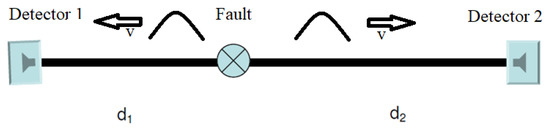
Figure 1.
Transmission line with a short and detectors.
If the unknown time at which the fault occurred is and the constant velocity of the signal propagation is v, the following relations follow:
in which and are the unknown distance from the fault to Detectors 1 and 2, respectively. The total distance between the two detectors is known as:
Defining the time difference , the distance from Detector 1 to the short may be written as follows:
Hence, if is a random variable of the standard deviation , the corresponding standard deviation of is:
provided we assume that the velocity v is known. Now, can be evaluated as:
in which the covariance is given in terms of the following expectation value:
If the uncertainty in is uncorrelated with the uncertainty in , the covariance is null, and we have a simplified expression:
If , this will result in:
Thus, we can rewrite in terms of as follows:
Now, suppose that the data are sampled at intervals of T; if the signal is detected initially at time , this means that the signal arrived at any time between and . Since we do not have any information about what time the signal really arrived, we assumed that is a random variable distributed uniformly in the interval . The probability density function of is depicted in Figure 2.
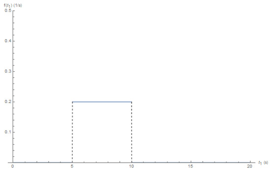
Figure 2.
Uniform distribution probability density function of ; in the illustration, we assumed and .
Since the moments of a uniform distribution function are known, we can easily evaluate the expectation and standard deviation of as follows:
Thus, the accuracy at which we need to know the location of the fault will determine the sampling rate according to the following formula:
As we shall show later, for a power line, the typical propagation of the signal is close to light’s velocity in a vacuum:
Thus, if the required distance precision is about 1 m, then the time measurement sampling rate should be:
This is much lower than the clock rate of current computer processors. We do not deal here with additional sources of uncertainty, such as the noise level of transmission lines, and leave that for future work.
3. Methodology: Signal Detection
What kind of signal should we measure for the fault location, and should it be the voltage or current? How should it be processed in order to avoid the accumulation of a large amount of unnecessary data due to the high sampling rate dictated by Equation (14)? We shall try to answer those question using a lumped circuit model, as described in Appendix A [26,27,28], in which we show that a fault signal can be obtained by measuring either the current or voltage.
The high sampling rate that is needed for accurate location as described in Equation (12) imposes a storage challenge as the amount of data accumulated may be prohibitive. However, taking the derivative of the signal, which may be the voltage or current, allowed us to overcome this obstacle (see Appendix A). By choosing a high detection threshold, one avoids false positives, and this allowed us to store a relatively small amount of data that was sufficient for the detection and location of the short. In some cases, a second derivative was required.
Generally, the first voltage derivative is enough (except for the load voltage), while in the case of current measurement, the second derivative is necessary.
We further noticed an additional restriction on the required resolution T, in order to avoid the case that the pulse goes undetected, that is between sampling points, we needed to have a resolution smaller than the pulse duration, which is the same duration as the time it takes the short to form; hence:
Now, if s, this means that:
This limitation is even more restrictive than the one appearing in Equation (14), leading to:
Obviously, a lumped model neglects the effect of spatial distances, and hence the effect of signal propagation. To describe the effect of signal propagation properly, a distributed model is needed, and with such a model we could study the short signal propagation and related phenomena including dispersion; this is discussed in the following section.
4. Methodology: Distributed Model
Until now, we have ignored the signal propagation in the circuit and assumed that the changes in the voltage and the current occur immediately and simultaneously everywhere. This assumption is not compatible with the theory of special relativity, which states that any signal must propagate with finite velocity, smaller than the speed of light in a vacuum [1]. To describe this behavior, we used the transmission line propagation model [29], a section of which is depicted in Figure 3.
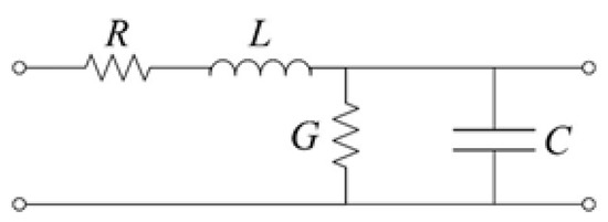
Figure 3.
Transmission line structure for a single unit length.
This approach leads to the telegraph equations. We describe this model in the time and frequency domains and draw the relevant conclusion from each presentation.
4.1. The Time Domain
The equations that describe the voltage and the current dependence in the time domain are the telegraph equations given below [29]:
where R is the resistance, L is the inductance, G is the conductance, and C is the capacitance, per unit length each (see Figure 3). This pattern is repeated indefinitely (see Figure 4).
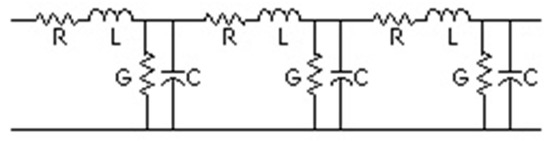
Figure 4.
Transmission line structure repeated.
The above equations can be solved for an infinite transmission line excited at by an excitation representing the effect of the short on the voltage. The solution for the voltage is:
The above solution describes a voltage signal propagating at a velocity:
and an exponential decay with a decay factor of:
Assuming the transmission line to be a two-wire cable as described in Appendix A, the following parameters are obtained [29]:
where each wire has a diameter d, and the distance between the wires is D. The material between the wires has a permittivity , permeability , and (a very small) conductivity . The wire resistance is calculated, as in Equation (A6), using the surface resistance given in Equation (A5). The short propagation velocity (20) can be now calculated using the parameters of Equation (22), to yield:
where n is the index of refraction around the transmission line. It should be noted that the electromagnetic wave is propagating in the region between the conductors and not in the conductors themselves, where the propagation is much slower and the decay is very strong. We noticed that if the two wires are surrounded by air , we would recover the velocity of Equation (13).
Notice that since according to Equations (A5) and (A6), the resistance is frequency dependent as dictated by the skin effect, the resistance term in Equation (18) is not a simple multiplication and should be replaced by a convolution. Thus, a frequency domain formalism is more adequate for this type of problem, as will be described next.
4.2. The Frequency Domain
In the frequency domain, the telegraph equation takes the form [29]:
Combining these two equations, we can separate the voltage and current variables, in terms of the following two equations:
where we define:
These equations have a solution of the form:
The functions are derived from the initial conditions. The impedance is defined as follows:
In the case where the resistivity and the leakage admittance are small enough, such that:
we can approximate the impedance:
and the real and imaginary parts of take the form:
As the frequency rises, the approximation becomes more accurate. Hence, for the higher-frequency Fourier components associated with the short formation, this approximation is more effective. Notice that while describes absorption and coincides with the same expression for absorption obtained in Equation (19), describes propagation.
4.3. Time-Dependent vs. Stationary Shorts
Steady-state shorts are easily analyzed in transmission line theory; here, we shall try to elucidate the connection between the transient phenomena of the short’s appearance and its asymptotic behavior as a steady- state phenomenon. Our model is depicted in Figure 5.
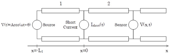
Figure 5.
Detailed short in the transmission line model.
We assumed that the short appears at some point () in the transmission line, in which the continuity of the voltage and current dictates:
We assumed that the short current does not exist at ; likewise, the short current after a long time can be calculated using the fact that the voltage on the short vanishes at . The second assumption can be formulated as:
To obtain the asymptotic short current, the following calculation was performed. First, we used the fact that after a considerable duration, the voltage on the short vanishes to obtain the following:
This leads to the result:
Inserting this result into Equation (27) and taking into account that is the source voltage lead to the following result:
Hence:
The asymptotic short current in the frequency domain can be calculated using Equation (27) at and taking into account Equations (35) and (37):
Taking into account given in Equation (A8) (which is equivalent to a sum of delta functions in the frequency domain), the asymptotic short current in the time domain is:
The second assumption was that the short current vanishes at :
In the current model, this requirement is fulfilled by multiplying the asymptotic expression with some reasonable function that vanishes at and approaches unity at , for example:
in which is a step function. The calculation results for the short current on the load side are as follows:
where , , and . v is the signal propagation velocity. The current at the load side is affected by three terms, each with unique retardation. The source voltage is retarded by a time , while the short current is retarded by a time for the direct signal and by for the same signal reflected by the circuit source. Each retardation time is proportional to the distance it needs to travel from its source and inversely proportional to the velocity of propagation. The model also shows that the signals suffer attenuation proportional to the distance they travel.
4.4. Signal Dispersion
We now consider the problem of dispersion. This problem is interesting since we would like to know in what ways does the line distort signals propagating on it and, in particular, how the signal produced by the short is effected. We start from the definition of given in Equation (26), and we assume that . Consequently, the propagation index is:
Now, let us investigate the condition:
The resistance is frequency dependent due to the skin effect and can be calculated from the surface resistance using Equations (A5) and (A6) as follows:
Thus, we obtain the ratio:
Thus, the approximation given in Equation (44) is even better for higher-frequency components. Introducing the inductance impedance:
we can cast Equation (46) in the form:
in which the numerical values for the parameters are taken from Table A1, Table A2, and Table A5. Equation (48) is depicted in Figure 6, which shows that the condition given in Equation (44) holds even better for a high frequency.
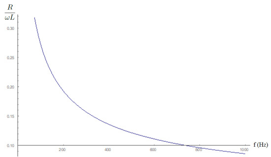
Figure 6.
The ratio of resistance to inductance impedance as a function of frequency according to Equation (48).
For a small parameter , we can write:
Hence, taking into account that , of Equation (43) has up to third order the form:
This expression can be separated into an imaginary and real parts as follows. The imaginary part of takes the form:
where we have taken into account Equation (46). As Equation (51) is linear in , we concluded that there is no dispersion during the signal propagation that requires non-linear phase terms. To appreciate the linearity of , we depict it as a function of the frequency in both Figure 7 for low frequencies and in Figure 8 for high frequencies without making an expansion approximation; the linearity and, hence, the lack of dispersion are apparent for a wide frequency range.
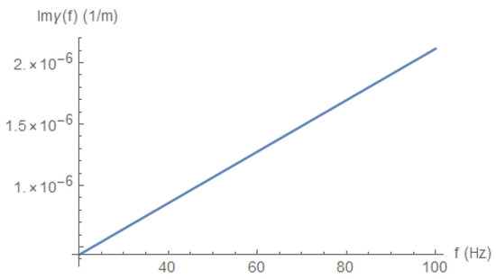
Figure 7.
low frequency dependence.
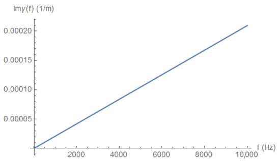
Figure 8.
high frequency dependence.
For the real part of , we obtain:
The real part depends on the frequency, but this part is relatively small, compared to the imaginary part. To appreciate the frequency dependence of , we depict its behavior for low frequencies (Figure 9), high frequencies (Figure 10), and extremely high frequencies (Figure 11).
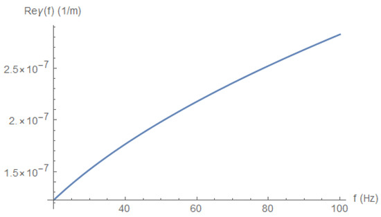
Figure 9.
for low frequencies.
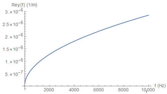
Figure 10.
for high frequencies.
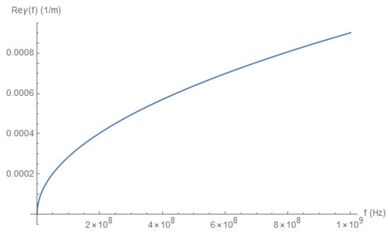
Figure 11.
for very high frequencies.
To appreciate how small is with respect to , we plot the ratio of those quantities in Figure 12.
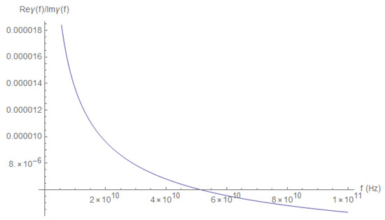
Figure 12.
The ratio of the real part to the imaginary part of .
Another indication of the dominance of over is the frequency dependence of , which follows quite closely the linear behavior of , as depicted in Figure 13.
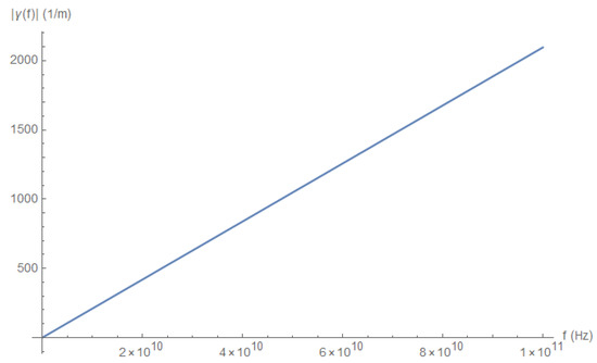
Figure 13.
as a function of frequency.
Finally, we remind ourselves that we assumed zero admittance in our calculations. Practically, this means that we neglected the air admittance with respect to the capacitive admittance:
To check if this assumption is justified, we calculated the ratio of the air admittance to capacitive admittance:
where we used the parameters of Table A3 for the air admittance and Equation (22) for the capacitance. The ratio, which is quite small, becomes even smaller for higher frequencies, as depicted in Figure 14, and thus justifies our initial assumption.
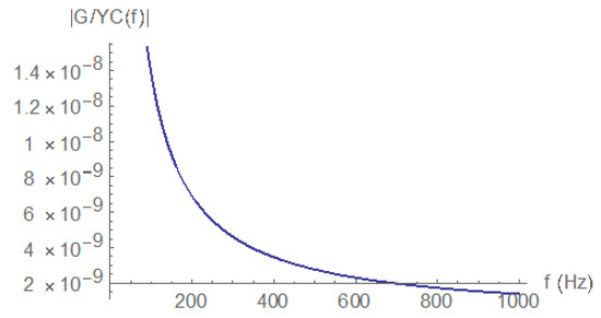
Figure 14.
The frequency dependence of .
The conclusion of this subsection is that dispersion is not significant in the media in which the pulse generated by the short propagates. This will be further elaborated in the next subsection, as we study the prorogation of a signal along the line.
4.5. Signal Propagation
We assumed that at the entrance to a transmission line, we inject a short signal of the form:
Thus, we assumed that the short generates a pulse signal, while the standard voltage is a periodic trigonometric function of frequency , which is modulated by the pulse. The pulse was assumed to be Gaussian with a width . The same signal in the frequency domain takes the form:
This signal is depicted in Figure 15.
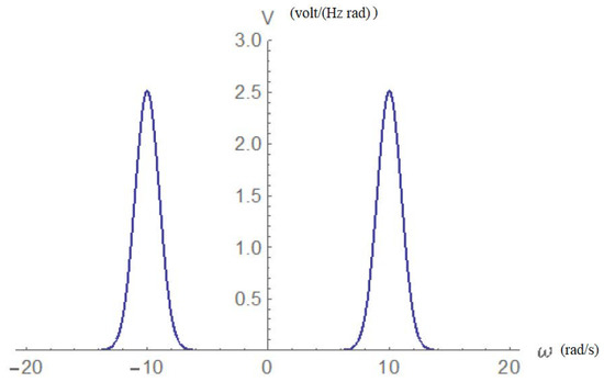
Figure 15.
The entrance voltage signal in the frequency domain.
Now, since that signal is injected at the entrance, it can propagate in only one direction; hence, Equation (27) takes the form:
We now expand around till the second order. This results in:
Taking into account Equations (56)–(58) and performing an inverse Fourier transform, we arrive at the following expression for a propagating signal:
where the delay time is:
hence, this is approximately the distance divided by the velocity, as expected. We noticed that the expression:
is the group velocity, which is the velocity of a wave packet. The width of the signal is:
where:
The term signifies the pulse broadening as it propagates along the line. Let us assume that s. For a frequency of 1 MHz and a distance of 1 km:
hence, the dispersion is negligible. However, for a frequency of 1 kHz and a distance of 10 km:
the widening is comparable to the initial width. Hence, despite the fact that dispersion seems small, it accumulates over long distances.
4.6. Bifurcations
A power transmission line often bifurcates, as depicted in Figure 16.
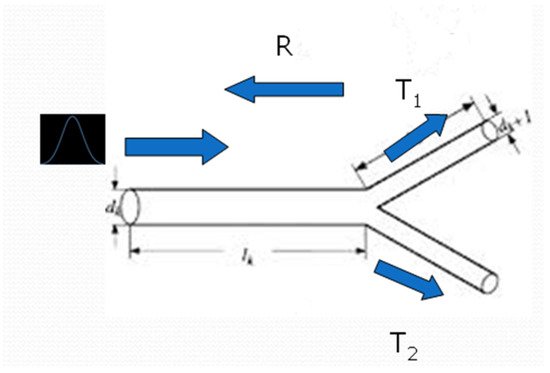
Figure 16.
Schematic bifurcation in a power line.
In the bifurcation junction, the signal is transmitted to the bifurcating channels and is also reflected to the original channel in which the short was originally formed. The amount of signal reflected or transmitted is quantified by the reflection R and transmission T coefficients. Those coefficients can in turn be calculated as follows:
in which is the impedance of the line before the bifurcation junction and is the impedance of the line after the bifurcation junction. In case the signal meets multiple bifurcation junctions along its path, multiple reflection occur, as depicted schematically in Figure 17.
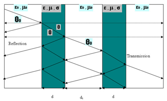
Figure 17.
Multiple reflections from a changing propagation media.
Multiple reflections will result in multiple signals arriving at the detector, as depicted schematically in Figure 18.
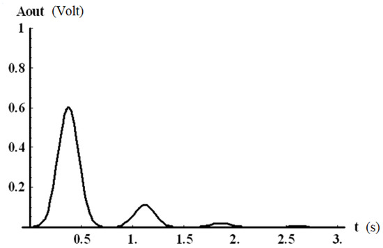
Figure 18.
Multiple reflections arriving at the detector.
We note that reflected signals arrive at the detector later and in reduced amplitude due to the longer path they need to travel and the additional attenuation the signal suffers during propagation (see Equation (59)) and reflection. We note that if a line bifurcates into multiple identical lines as in Figure 19, the total impedance at the channel after the bifurcation will be equal to the original impedance divided by the number of transmission lines N; hence:
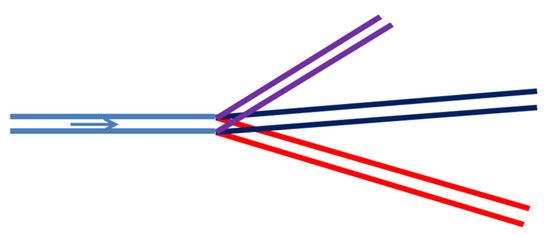
Figure 19.
A transmission line bifurcating into multiple channels.
This implies, according to Equation (66), a transmission coefficient of:
hence, for a bifurcation to a large number of channels, the reflection coefficient will tend to one, while for a continuation into a single identical channel, there will not be obviously a reflection.
We now examine the reflection effect and see if one can use the reflected signal instead of a second sensor, thus reducing the amount of hardware needed in order to implement the method described. First, let us look at Figure 20: The short occurs between the sensor and the bifurcation point. Thus, a signal is propagating from the short to the sensor, and an additional signal propagates to the bifurcation point where it is reflected. Provided that the short will not introduce an impenetrable obstacle, the signal will eventually reach the detector at a later time. The direct signal arrival time will be satisfied according to Equation (1):
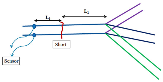
Figure 20.
A short occurs between the sensor and the bifurcation point.
The reflected signal will arrive at a later time such that:
Hence, the time difference between the direct and reflected signal allowed us to calculate the distance between the short and bifurcation point as:
Now, since the distance L between the sensor and the bifurcation point is known in advance, we may calculate the distance between the short and the bifurcation point as follows:
Thus, in this case, a single detector will suffice, and we will not need two detectors, as described in Section 2. This reduces the cost of the system and removes redundant issues such as sensor synchronization. The last advantageous scenario is depicted in Figure 21.
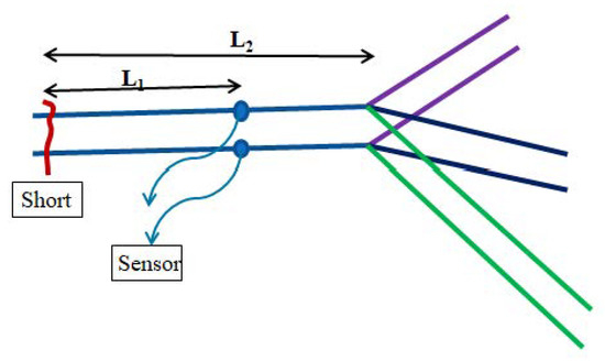
Figure 21.
The sensor is between the short and the bifurcation point.
The direct signal arrival time will be satisfied according to Equation (1):
The reflected signal will arrive at a later time such that:
The time difference in this case will yield:
which does not reveal any information about the short location, but rather, some trivial information about the distance between the sensor and the bifurcation point, which is already known. Of course, if there exist additional bifurcation points on the signal path (for example, left to the short), then we are in the previous case again, and one sensor will suffice. We may deduce that putting sensors on bifurcation points will reduce the amount of sensors needed. Finally, we looked at the case in which the signal arrives at a sensor located after the branching point of the net, as in Figure 22.
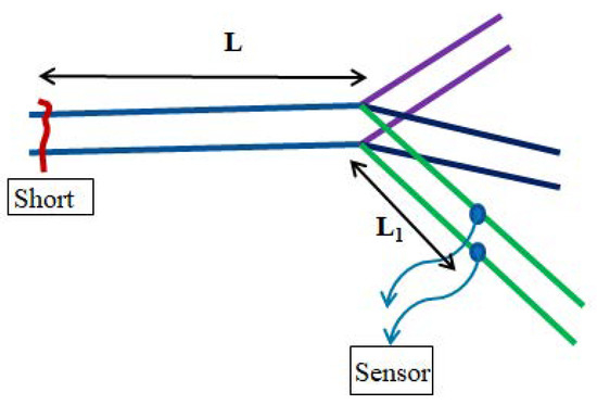
Figure 22.
The sensor is on a bifurcation of the transmission line.
The sensor will receive a signal at:
This will not suffice to locate the short unless a reflected signal is received from another point along the network. To conclude, we deduced that putting sensors on bifurcation points will reduce the amount of sensors needed along the network. Moreover, relying on reflections may solve the problem of sensor synchronization.
4.7. Laplace Analysis
We now address the transmission line pulse propagation problem using the technique of Laplace analysis [30]. The simplified power system of our interest is schematically presented in Figure 23.
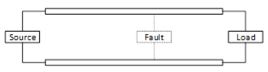
Figure 23.
Schematic of the fault scenario.
The fault produces two separate signals propagating towards the source and the load, where the sensors are located. In each section, as a result of the fault, the voltage perturbation is perceived as an input signal, propagating towards a sensor, as shown in Figure 24.
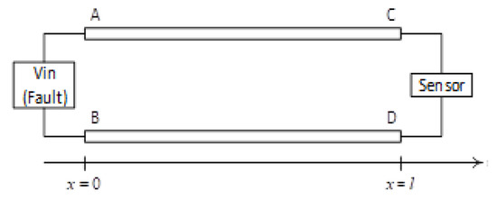
Figure 24.
Schematic of the fault modeling.
In the transmission line, we assumed the validity of the telegraph Equation (24) and replaced . The Laplace form of the telegraph equations admits the solution:
where,
It is realistic to presume that the conductance G of the separating dielectric material between the wires is insignificant. The series resistivity is calculated taking into account the skin effect:
where d is the conductor wire diameter and:
Consequently, the expression (82) can be written as follows:
The sensor impedance was designed to be infinite so as not to influence the measurement results. Substituting boundary conditions,
and:
which implies zero current at :
or:
The voltage signal at the sensor due to the fault is thus:
Identifying the last expression as the summation of a geometric series, it can be re-written as the sum:
This sum can be interpreted as the sum of multiple reflected waves each with its unique delay time. The system’s transfer function may be now calculated as follows:
This allows for obtaining the signal measured at the sensor, due to any fault waveform. For example, if the fault is a sudden short circuit at and , the voltage at the fault location is:
Using the superposition principle, may be expressed as the sum of a DC input and a step function input response.
Since the impedance at the edge is infinite, the voltage along the line due to the DC input is simply . Moreover, the Laplace transform of a step function satisfies:
hence:
Hence, using the transfer function definition, Equation (98), and performing an inverse transform back to the time domain, we obtain:
Taking a known inverse Laplace transform [22]:
The voltage at the sensor, as a result of the fault, is:
The above result will suffice if the rise time of the short is fast enough and can be ignored.
5. Methodology: Experimental Setup
5.1. Experiment Hardware
The experimental demonstration of the fault location technique involved the setup shown schematically in Figure 25, in which a 10V DC voltage was supplied from a TTi QL355TP power supply source, shown in Figure 26, to a 50 m two-wire cable and switches. The sensor was a MS09404A Mixed Signal Oscilloscope with a 4 GHz bandwidth, which has two channels, as shown in Figure 27.
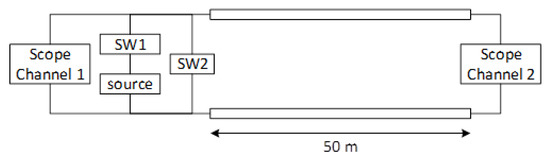
Figure 25.
Schematic of the experimental setup.
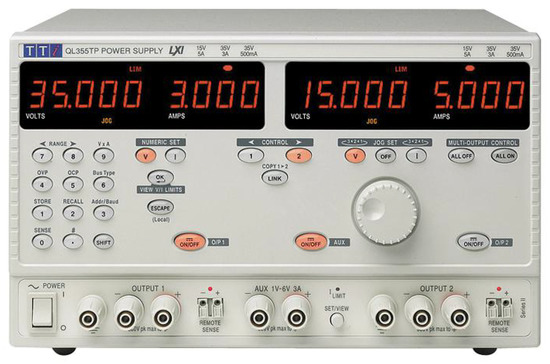
Figure 26.
TTi QL355TP power supply.
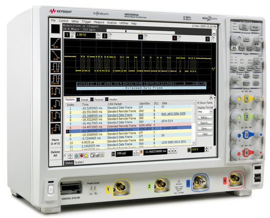
Figure 27.
MS09404A Mixed Signal Oscilloscope of a 4 GHz bandwidth having two channels.
Figure 28 illustrates the dimensions of the transmission line.
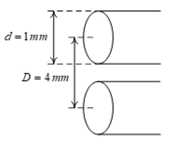
Figure 28.
Dimensions of the transmission line.
The transmission line was comprised of a two-wire power cord. Each wire was made of copper and had a mm diameter, while the distance between the wires was mm. These parameters allowed us to calculate the inductance L and capacitance C from the dielectric constant, magnetic permeability, and conductivity as follows (see Equation (22)):
5.2. Experimental Process
On one side of the transmission line, we connected the DC source, 2 switches, and the scope channel; another channel was connected to the other side. Closing the first switch when the second switch is open, we obtained a steady-state DC voltage along the line. The short circuit fault was achieved by closing the second switch.
6. Results: Data Processing
6.1. Location Accuracy
Measuring the voltage of both sides of the line, we can see clearly the delay in signal propagation along the line. Additional reflected waves (Figure 29 and Figure 30) are also seen. The scope channel data were exported and processed using the MATLAB software.
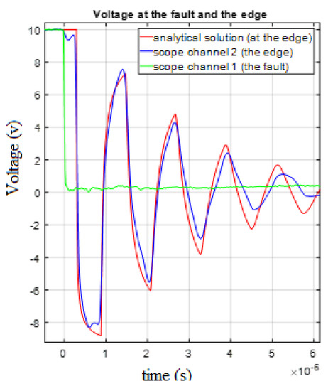
Figure 29.
Comparison of the experimental results and theoretical predictions of Equation (105) for the measured voltage.
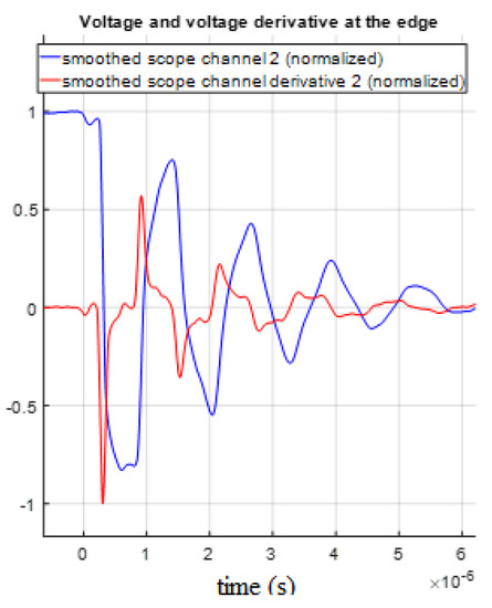
Figure 30.
Comparison of the sensor voltage and its derivative.
Our aim was of course to discover how long it takes the signal to arrive from the fault to the measuring point. Because the waves arriving at the edge are reflected in the opposite direction (towards the fault), where they are repeatedly reflected, one fault may supply several data points that we can process to our advantage, depending on how fast the transient signals decay. In this study, it was possible to measure five signals (peaks) each time, and so, we chose the optimal data processing technique.
To obtain the best accuracy, we performed numerous voltage smoothing and voltage derivative smoothing, changing the time window and thus the number of samples. Obviously, the wider the window, the less noise we had to distort our results. However, a wide window may distort the reflection signal as well, compromising our accuracy. We used five different averaging windows and thus obtained five different errors for each reflection. The data are given in the Appendix B; in the table, each line represents a different value of the voltage smoothing window and voltage derivative smoothing window and the errors that were deduced for each reflection and processing method.
Figure 30 shows that the voltage derivative peaks were much sharper; therefore, the short circuit fault location was calculated by finding the time intervals between the local extremum points in the voltage derivative at the transmission line edge. In addition, the smoothing filter window may slightly change the results, and the optimum configuration was 200 points in a window. In this situation, the accuracy in the short circuit fault location detection was 0.005% using the second peak.
This can be compared to the theoretical accuracy predicted by Equation (11). In the current case, the sampling rate was 4 GHz, and hence, the time between samples was s and the velocity m/s. Thus, the accuracy may be as high as 0.008 m, which is 0.008%, quite close to the best experimental result. This indicates that the theoretical limit is achievable provided the data are processed correctly.
6.2. Comparison with Theory
We now compare the results of the theory given in Equation (105) to the (smoothed) experimental results. The signal reflection scheme is shown in Figure 31. The results of the comparison are depicted in Figure 32.
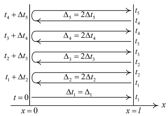
Figure 31.
The propagation times for the pulse reflections.
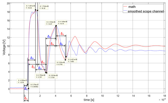
Figure 32.
Comparison results between Equation (105) and the smoothed scope channel.
The unprocessed timings of various peaks were correlated with signal reflections and are given in Table 1.

Table 1.
Distance calculations based on raw data without applying any processing technique.
The same results derived from the theoretical calculation are given in Table 2.
Table 2.
Distance calculations from the simulation results.
Obviously, the theoretical distance evaluation was better than the experimental one; however, processing dramatically improved the situation, as we saw in the previous section. The distances can be derived from the time differences since = m. In the above, we denote and for one-direction experimental and theoretical propagation times, respectively. As we can see, the propagation times were sufficiently stable and consistent with the theoretical model. Hence, the pulse location information can also be obtained from the voltage signal (without the signal derivative if precision is not required).
However, there was a difference between the theoretical and the experimental graphs. In the experimental data, there were additional peaks in the first reflected waves; after the third (main) peak, the “oscillation” frequency was twice as great as in the theoretical model. This was because of the reflected waves from the middle of the transmission line: in the experimental setup, the line was not homogeneous, as can be deduced from the additional peaks we received.
Finally, we present the comparison of the theoretical and empirical derivatives given in Table 3 and Figure 33. The timing of the peak derivatives seemed to fit much better the theoretical curve, and the location errors were much smaller. As noted previously, processing may improve the accuracy drastically.
Table 3.
Distance calculations from the signal derivatives and respective location errors.
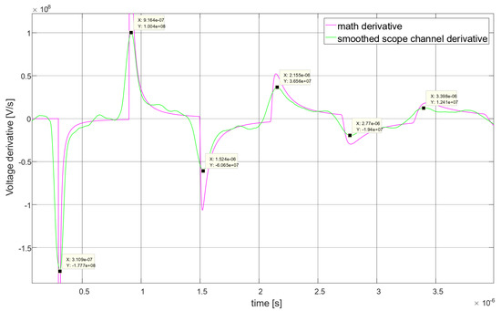
Figure 33.
Comparison between the theoretical derivative and smoothed scope channel derivative.
7. Synchronization between Sensors
In order to take full advantage of the accuracy of the current method (see Table 4 and [2,3,4,31,32,33]) proper synchronization between sensors is required. Indeed, before measuring a transient phenomenon [34], an accurate method for measuring it must be chosen [35]. According to a broad literary review of a shelf product that will be used in the final device for synchronization between the measurements of the sensors, it was found that the White Rabbit Precision Time Protocol (PTP) was suitable for robust sub-nanosecond synchronization [36]. For a description of the characteristics of this technology, see [37,38,39].
Table 4.
Comparison of fault location accuracy methods. DSE—distribution state estimation algorithm. SMT—synchronized measurement technology.
8. Conclusions and Summary
In the framework of the current research, a propagation of a short signal in a two-wire cable was investigated. It was shown that the short can be detected either by voltage or current measurements using the voltage/current first or second derivatives. The short can be detected either at the source or the load side. It was also shown that using bifurcations and reflection, the amount of detectors may be reduced. In order to achieve a high level of accuracy regarding the short’s location, the inter-sampling duration should be of the nanosecond order (GHz sampling frequency). Of course, if there is no significant slope over a predetermined number of samples (say 1000 samples), there is no need to save them. Hence, the samples may be written as a moving window to some buffer register and deleted if the gradient is not significant. We also studied the phenomena of the dispersion of the short signal and determined in what cases it was significant.
Our method was based on the idea that in any system information even in the form of an electromagnetic wave will advance from one side of the system to the other in a fast, but finite velocity v stratifying , where c is the speed of light in a vacuum. When considering a steady-state, we may neglect the propagation phenomena and employ lumped models; however, this is not applicable for short durations, as considered here.
The accuracy was significantly better in the retardation approach than in various methods mentioned in previous work. In Table 4, the accuracy of the different methods is compared.
It is expected that in the future, better wave sampling techniques and devices will be developed, as well as better processing methodologies, thus improving accuracy.
As the temporal difference between the fault signal arrivals and the width of the signal (see for example Figure A37) are much less by many orders of magnitude than the period of the AC voltage, one can assume that for all practical purposes, the AC signal is constant. Hence, we expect an AC experiment to yield similar results.
The above system description was derived for an electrical transmission line as the wave behavior is well known and there is considerable expertise in making the calculations; however, the same holds true for optical fibers and optical reflections, as well as for pipes, such as water, gas, or oil pipes, for which one can use acoustic echoes. The calculations for the fault’s location are the same, although the propagation rates are different in the acoustic case. In the optical case, the equation still holds true. In both cases, underground pipes and underground fiber optic cables can be damaged at hard-to-reach locations, and an accurate determination of the fault’s location is helpful in knowing where to start digging.
Author Contributions
Conceptualization, A.Y. and Y.P.; methodology, A.Y. and Y.P.; software, A.Y. and M.S.; validation, A.Y. and Y.P.; formal analysis, A.Y., Y.P. and M.S.; investigation, A.Y., Y.P. and M.S.; resources, A.Y. and Y.P.; data curation, M.S.; writing—original draft preparation, M.N.; writing—review and editing, A.Y.; visualization, A.Y., Y.P. and M.S.; supervision, A.Y. and Y.P.; project administration, A.Y. and Y.P. All authors have read and agreed to the published version of the manuscript.
Funding
This research received no external funding.
Institutional Review Board Statement
Not applicable.
Informed Consent Statement
Not applicable.
Data Availability Statement
Not applicable.
Conflicts of Interest
The authors declare no conflict of interest.
Appendix A. The Lumped Circuit Model
The schematic description of the short circuit is presented in Figure A1.
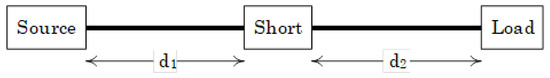
Figure A1.
Transmission line with a short.
This is modeled in Figure A2.
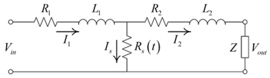
Figure A2.
Short circuit example.
The parts of the transmission line before and after the short circuit are considered as a resistor and inductor connected in series. In order to mathematically analyze this, we used the Kirchhoff voltage law and Ohm’s law:
in which is the source voltage, is the source current, is the short voltage, is the load current, and is the load voltage. and are the resistance and inductance before the short, and and are the resistance and inductance after the short, while Z is the load impedance.
Appendix A.1. The Case of Resistive Impedance
In the first step, we ignored the inductance for mathematical simplicity. We also noticed that by Ohm’s law:
where is the time-dependent short resistance and is the current flowing through the short. According to Kirchhoff’s current law:
Thus, the currents in this case can be calculated algebraically as follows:
In the current model, the transmission line was a two-wire copper cable; each wire has a diameter d, and the distance between them is D; the cable is depicted in Figure A3. The total cable length is l. The values used for the demonstration are given in Table A1.
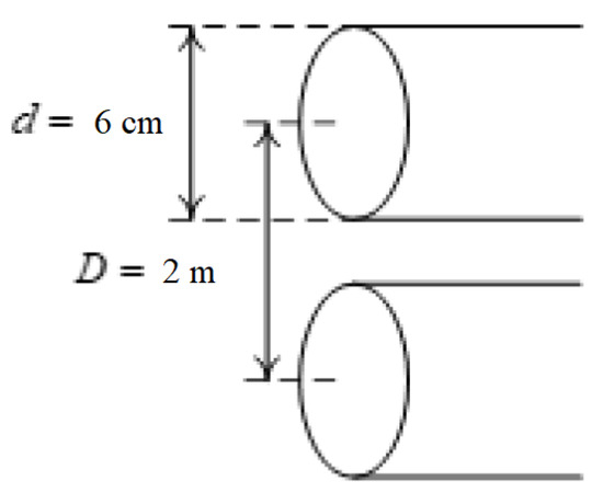
Figure A3.
Cable geometry for the demonstration.
Table A1.
Two-wire cable parameters.
Table A1.
Two-wire cable parameters.
| Parameter | Value | Unit |
|---|---|---|
| (Copper) | S/m | |
| d | 0.06 | m |
| D | 2 | m |
| l | 1000 | m |
The surface resistance in ohms () may be written as follows [29]:
In the above, is the angular frequency, f is the frequency, is the magnetic permeability of the material, and is the conductivity. Hence, the resistance per unit length can be written as:
The values used for the cable description appear in Table A2.
Table A2.
Two-wire cable resistance.
Table A2.
Two-wire cable resistance.
| Parameter | Value | Unit |
|---|---|---|
| H/m | ||
| f | 50 | Hz |
We noticed that the value of Hz used above is typical for many power lines. However, as the typical duration of the short is miniscule, the signal generated by the short will include a broad band of frequencies, each suffering a different impedance. This is dealt with in a later part of this paper. However, here, we assumed for simplicity that the resistance is constant.
The short circuit appears at distance from the input. The short-circuit resistance is shown in Figure A3. The short is described by a time-dependent resistance, which was assumed to behave exponentially:
The initial resistance was assumed to be very large and represents the region’s air resistance. However, at time , a short is initiated, causing an exponential decrease in the short resistance at a typical duration of = 10–100 ns, which depends on the conditions and geometry of the short-circuit region. The short-circuit parameters are concentrated in Table A3.
Table A3.
Short-circuit parameters.
Table A3.
Short-circuit parameters.
| Parameter | Value | Unit |
|---|---|---|
| 300 | m | |
| 700 | m | |
| 100 | ns | |
| (air) | Ωm | |
| 0.1 | m | |
| 0.0004 | ||
Thus, the current flows through the short instead of the load, causing a decrease in the load current. Moreover, since the overall impedance of the circuit decreases and is now dominated by the impedance of the short, the current at the source becomes much higher.
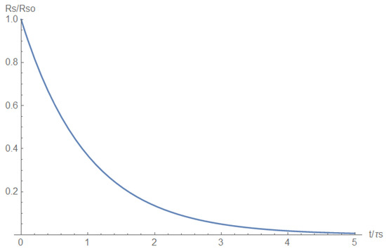
Figure A4.
Short-circuit resistance.
The transmission line resistances and the load impedance are described in Table A4.
Table A4.
Transmission line resistance and load impedance.
Table A4.
Transmission line resistance and load impedance.
| Parameter | Value | Unit |
|---|---|---|
| 0.00579 | ||
| 0.0135 | ||
| 0.0193095 | ||
| Z | 15.625 |
The input voltage was assumed to be of the form:
where = 220 [V], rad/s. We shall now present the calculation results.
Appendix A.1.1. Current
The source current just before the short is depicted in Figure A5 and after the short is depicted in Figure A6.
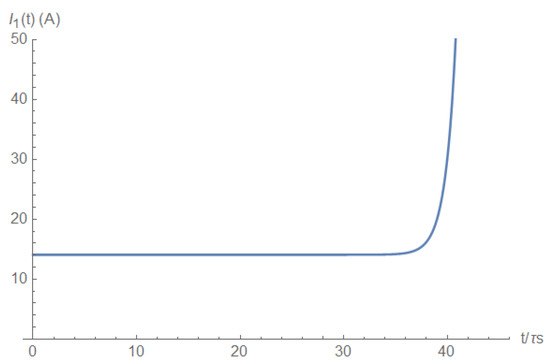
Figure A5.
Source current before the short.
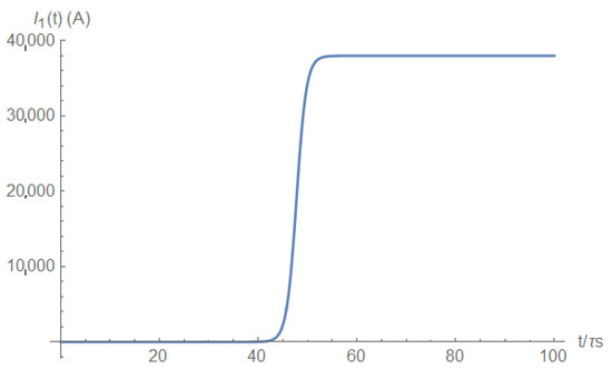
Figure A6.
Source current after the short.
Hence, the current at the source is a highly sensitive indicator of the occurrence of a short. To avoid storing unnecessary data and for precise timing of the short’s occurrence, one can look at the source current derivative (Figure A7); this has a distinctive pulse shape. Hence, by taking the derivative of the signal and by fixing a high detection threshold, one can avoid recording unnecessary data.
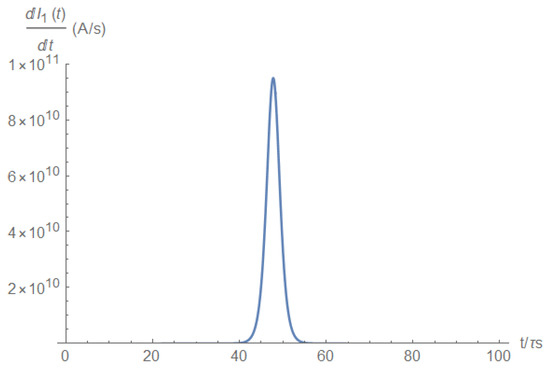
Figure A7.
Source current derivative.
On the load side, the current vanishes after the short occurs (Figure A8); hence, the load current is also an excellent indicator of the short’s occurrence.
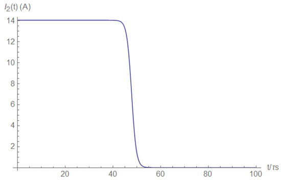
Figure A8.
Load current.
Again, we see that on the load side, the current behavior allows for identification of the short by taking the current derivative (Figure A9). This method allows precise timing with the need to store a small amount of data, as indicated above.
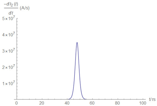
Figure A9.
Load current derivative.
Appendix A.1.2. Voltage
The short circuit pulse may also be detected by the voltage measurement. For example, the voltage measured at half the distance between the source and the short will yield a voltage as follows:
This voltage is depicted in Figure A10.
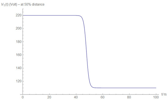
Figure A10.
Voltage at half the distance between the source and the short.
Again, the distinctive pulse shape of the voltage derivative (Figure A11) is apparent with the same advantage mentioned before.
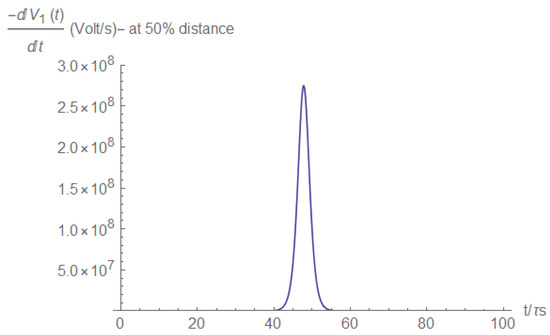
Figure A11.
Voltage derivative at half the distance between the source and the short.
The voltage at the short vanishes (Figure A12), since the resistance approaches zero during the short’s creation, providing the same behavior, which allows the pulse form in the voltage derivative (Figure A13).
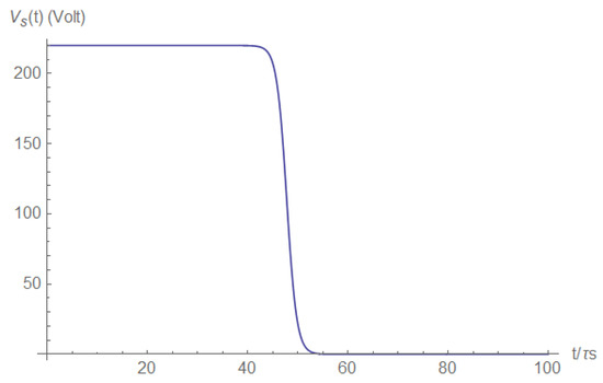
Figure A12.
Voltage at the short.
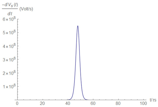
Figure A13.
Voltage derivative at the short.
Similarly, the voltage at half the distance between the short and the load may be measured (Figure A14), and the pulse may be detected using the voltage derivative (Figure A15).
Figure A14.
Voltage at half the distance between the short and the load.
Figure A15.
Voltage derivative at half the distance between the short and the load.
Summarizing the results of our first model, we saw that the current and voltage measurements enabled the short’s pulse detection, indicating the short’s occurrence. Likewise, it was shown that detection was possible both at the source and the load side. In order to detect the pulse, a resolution of the order is needed. In the current model, the inductance was neglected, leading to a simplified description; in the next section, we will look at the case were induction is taken into account, leading to a somewhat more complex mathematical analysis. Moreover, in a lumped model, there is no pulse propagation along the transmission line, and for this purpose, we introduce a distributed model later in this paper.
Appendix A.2. The Case of Resistive and Inductive Impedance
In this model, the transmission line inductance is no longer neglected as in the previous section. Therefore, the equations given in (A1) become coupled differential equations that can only be solved numerically. The two-wire cable induction can be calculated and is shown in Table A5.
Table A5.
Transmission line inductance.
Table A5.
Transmission line inductance.
| Parameter | Value | Unit |
|---|---|---|
| 0.000503938 | H | |
| 0.00117585 | H | |
| 0.00167979 | H |
The current in the circuit before the short occurs can be calculated analytically and is given as follows:
where: . This current is depicted in Figure A16.
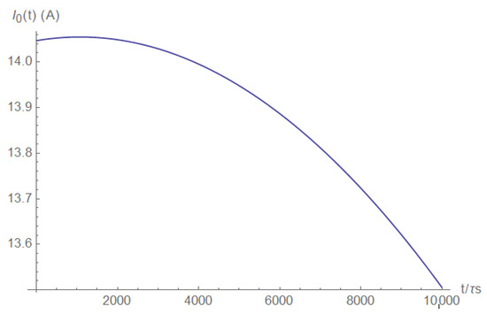
Figure A16.
The initial current.
We now study the numerical solutions of Equation (A1) given the above initial form.
Appendix A.2.1. The Current
The source current is demonstrated in Figure A17 (right after the short) and Figure A18 (a long time after the short).
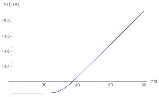
Figure A17.
Source current right after the short.
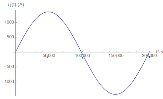
Figure A18.
Source current a long time after the short.
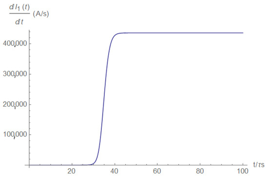
Figure A19.
The source current derivative.
In the previous model, the derivative had a pulse shape. In the current model, the first derivative did not exhibit a pulse shape (Figure A19); however, the second derivative (Figure A20) did exhibit a pulse shape with all the benefits mentioned previously.
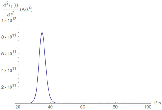
Figure A20.
The source current second derivative.
Current measurements on the load side also provide the short pulse detection ability. The load current is shown in Figure A21 (right after the short) and Figure A22 (a long time after the short). Here, the current decay is evident.
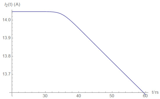
Figure A21.
Load current (right after the short).
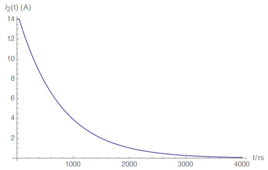
Figure A22.
Load current (after some time).
The current’s first and second derivatives are shown in Figure A23 and Figure A24, respectively.
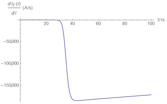
Figure A23.
The load current derivative.
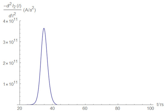
Figure A24.
The load current second derivative.
We see that the short may be detected and accurately timed by the current’s second derivative, measured at either the source or the load side. Next, we investigated the current at the short itself. It is obvious that it is zero before the short happens, after which it grows linearly (Figure A25). After some time, the short current reaches the characteristic source current values (Figure A26).
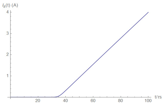
Figure A25.
Short current (right after the short).
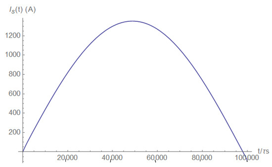
Figure A26.
Steady-state short current.
Appendix A.2.2. The Voltage
The short-circuit pulse may also be detected by the voltage measurement between the source and the short. If the voltage is measured at half a distance, due to a high short current, the voltage will be:
The voltage and its derivative are shown in Figure A27 and Figure A28, respectively. We deduced that for the voltage case, a first derivative will suffice for the short location even when inductance is not neglected.
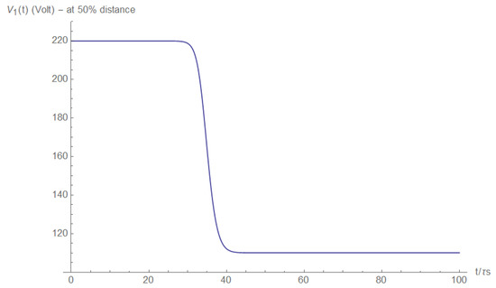
Figure A27.
Voltage at half the distance between the source and the short.
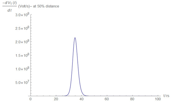
Figure A28.
Voltage derivative at half the distance between the source and the short.
Figure A29 and Figure A30 describe the voltage and its derivative at the short itself. We see that the voltage difference at the short when its resistivity goes to zero is also zero, and the pulse behavior of the voltage derivative is depicted.
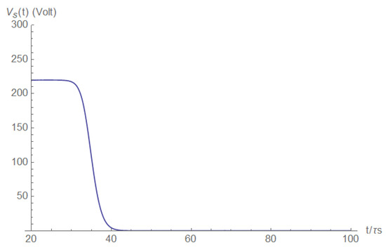
Figure A29.
The short voltage.
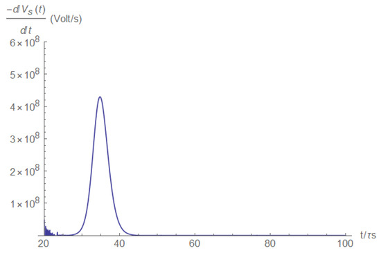
Figure A30.
The short voltage derivative.
Analogous results may be obtained if the voltage is measured at the load side, even if the measurement is not at the load itself. For example, for half the distance voltage measurement, one obtains:
Figure A31 and Figure A32 show the voltage at half the distance between the short and the load. The voltage a brief duration after the short has formed is depicted in Figure A31, and a longer duration of the same is depicted in Figure A32.
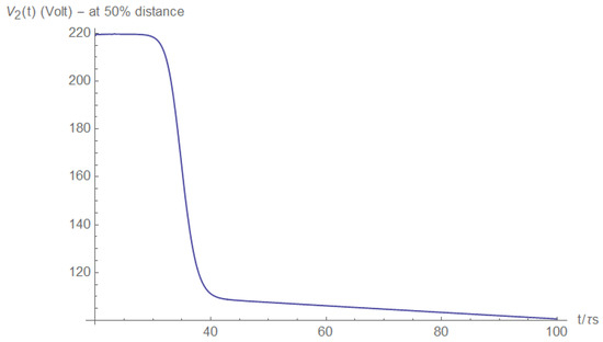
Figure A31.
Voltage at half the distance between the short and the load (right after).
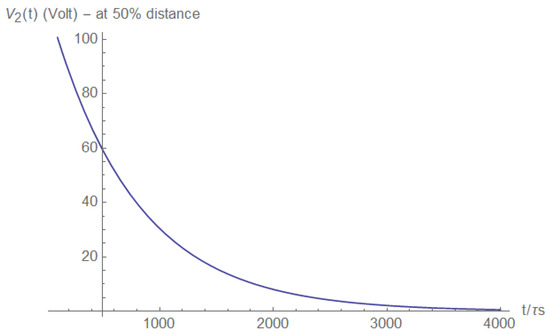
Figure A32.
Voltage at half the distance between the short and the load (after some time).
The voltage derivative displays a pulse behavior (Figure A33), and thus, in this case, a first derivative will suffice and a second derivative is not needed.
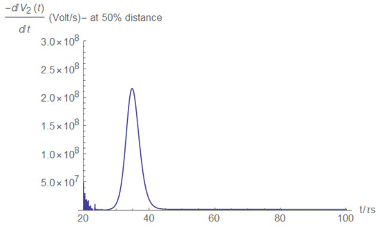
Figure A33.
Voltage derivative at half the distance between the short and the load.
Finally, the load voltage is described, which is proportional to the load current (see also Equation (A1)):
The load voltages, after a brief duration since the short’s occurrence and later, are shown in Figure A34 and Figure A35, respectively.
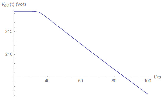
Figure A34.
Load voltage (right after the short).
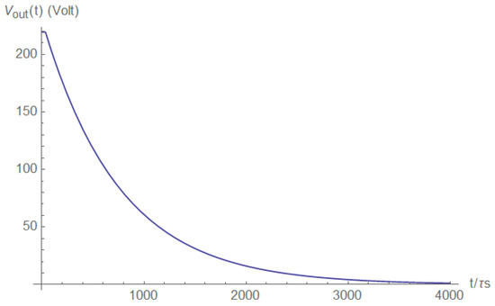
Figure A35.
Load voltage (after some time).
The first and the second load voltage derivatives are shown in Figure A36 and Figure A37. In this case, the desirable pulse shape was obtained for the second derivative.
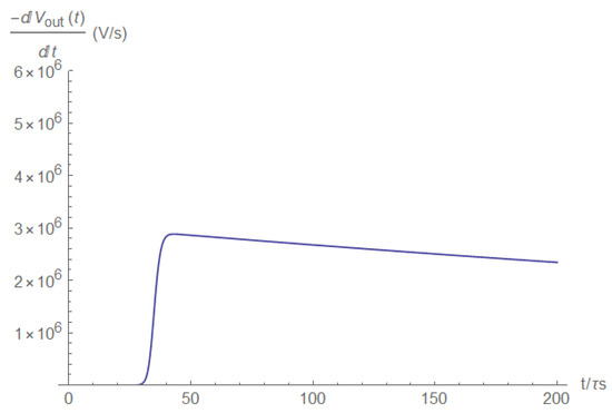
Figure A36.
Load voltage derivative.
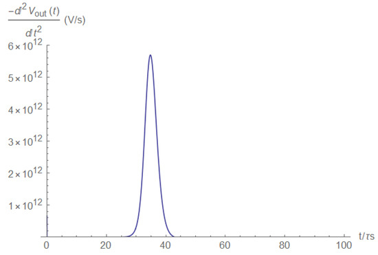
Figure A37.
Load voltage second derivative.
Appendix B. Errors Received from the Smoothing Voltage and Derivative Smoothing Voltage Window
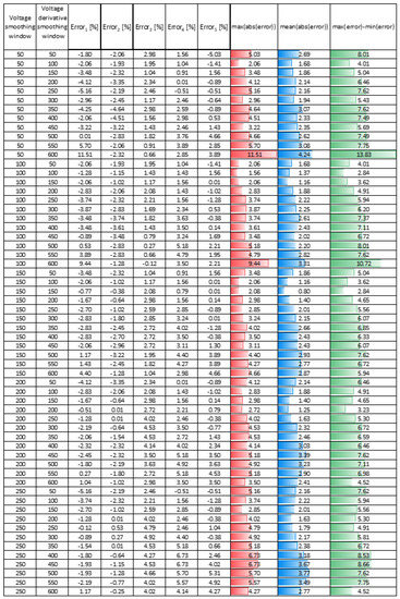
Figure A38.
Load voltage second derivative.
References
- Einstein, A. On the Electrodynamics of Moving Bodies. Ann. Der Phys. 1905, 17, 891–921. [Google Scholar] [CrossRef]
- Kulkarni, S.S. Fault Location and Characterization in AC and DC Power Systems. Ph.D. Thesis, University of Texas at Austin, Austin, TX, USA, 2012. [Google Scholar]
- Ghimire, S. Analysis of Fault Location Methods on Transmission Lines; University Of New Orelans: New Orelans, LA, USA, 2014. [Google Scholar]
- Xu, Z. Fault Location and Incipient Fault Detection in Distribution Cables; Western University: London, ON, Canada, 2011. [Google Scholar]
- Chen, K.; Huang, C.; He, J. Fault detection, classification and location for transmission lines and distribution systems: A review on the methods. High Voltage 2016, 1, 25–33. [Google Scholar] [CrossRef]
- Glik, K.; Rasolomampionona, D.D.; Kowalik, R. Detection, classification and fault location in HV lines using travelling waves. Prz. Elektrotechniczny (Electr. Rev.) 2012, 88, 269–275. [Google Scholar]
- Radojević, Z.M.; Kim, C.H.; Popov, M.; Preston, G.; Terzija, V. New approach for fault location on transmission lines not requiring line parameters. In Proceedings of the International Conference on Power System Transients Proceedings, Kyoto, Japan, 2–6 June 2009. [Google Scholar]
- Patel, M.; Patel, R.N. Fault analysis in transmission lines using neural network and wavelets. In Proceedings of the 2015 2nd International Conference on Signal Processing and Integrated Networks (SPIN), Noida, India, 19–20 February 2015; pp. 719–724. [Google Scholar] [CrossRef]
- Bunnoon, P. Fault detection approaches to power system: State-of-the-art article reviews for searching a new approach in the future. Int. J. Electr. Comput. Eng. 2013, 3, 553. [Google Scholar] [CrossRef]
- Dong, A.; Huo, L.; Liang, L.; Wang, Q. Research on the practical detection for a power cable fault point. In Proceedings of the 2010 International Conference on Computer and Communication Technologies in Agriculture Engineering, Chengdu, China, 12–13 June 2010; Volume 2, pp. 80–84. [Google Scholar] [CrossRef]
- Mustari, M.R.; Hashim, M.N.; Osman, M.K.; Ahmad, A.R.; Ahmad, F.; Ibrahim, M.N. Fault Location Estimation on Transmission Lines using Neuro-Fuzzy System. Procedia Comput. Sci. 2019, 163, 591–602. [Google Scholar] [CrossRef]
- de Morais Pereira, C.E.; Zanetta, L.C. Fault location in transmission lines using one-terminal postfault voltage data. IEEE Trans. Power Deliv. 2004, 19, 570–575. [Google Scholar] [CrossRef]
- Alam, M.N.; Bhuiyan, R.H.; Dougal, R.; Ali, M. Novel surface wave exciters for power line fault detection and communications. In Proceedings of the 2011 IEEE International Symposium on Antennas and Propagation (APSURSI), Pokane, WA, USA, 3–8 July 2011; pp. 1139–1142. [Google Scholar] [CrossRef]
- Srinivasarao, Y.; Pavani, S.; Sudharmi, G. Detection of Fault Location in Transmission Lines. Int. J. Appl. Eng. Res. 2017, 12, 1. [Google Scholar]
- Aldeen, M.; Crusca, F. IEE Proceedings-Generation, Transmission and Distribution. In Observer-Based Fault Detection and Identification Scheme for Power Systems; The Institution of Engineering and Technology: London, UK, 2016; Volume 153, pp. 71–79. ISSN 1350-2360. [Google Scholar] [CrossRef] [Green Version]
- Alsafasfeh, Q.; Abdel-Qader, I.; Harb, A. Symmetrical pattern and PCA based framework for fault detection and classification in power systems. In Proceedings of the 2010 IEEE International Conference on Electro/Information Technolgy, Normal, IL, USA, 20–22 May 2010; pp. 1–5. [Google Scholar] [CrossRef]
- Ashouri, A.; Jalilv, A.; Noroozian, R.; Bagheri, A. A new approach for fault detection in digital relays-based power system using Petri nets. In Proceedings of the 2010 Joint International Conference on Power Electronics, Drives and Energy Systems 2010 Power India, New Delhi, India, 20–23 December 2010; pp. 1–8. [Google Scholar] [CrossRef]
- Bhoomaiah, A.; Reddy, P.K.; Murthy, K.L.; Naidu, P.A.; Singh, B.P. Measurement of neutral currents in a power transformer and fault detection using wavelet techniques. In Proceedings of the 17th Annual Meeting of the IEEE Lasers and Electro-Optics Society, 2004, LEOS 2004, Boulder, CO, USA, 20 October 2004; pp. 170–173. [Google Scholar] [CrossRef]
- Dubey, R.; Samantaray, S.R.; Tripathy, A.; Babu, B.C.; Ehtesham, M. Wavelet based energy function for symmetrical fault detection during power swing. In Proceedings of the 2012 Students Conference on Engineering and Systems, Allahabad, India, 16–18 March 2012; pp. 1–6. [Google Scholar] [CrossRef]
- Shu, H.; Wang, X.; Tian, X.; Wu, Q.; Peng, S. On the use of S-transform for fault feeder detection based on two phase currents in distribution power systems. In Proceedings of the 2010 2nd International Conference on Industrial and Information Systems, Dalian, China, 10–11 July 2010; Volume 2, pp. 282–287. [Google Scholar] [CrossRef]
- Long, Z.; Younan, N.H.; Bialek, T.O. Underground power cable fault detection using complex wavelet analysis. In Proceedings of the 2012 International Conference on High Voltage Engineering and Application, Shanghai, China, 17–20 September 2012; pp. 59–62. [Google Scholar] [CrossRef]
- Magnusson, P.C.; Alexander, G.C.; Tripathi, V.K.; Weisshaar, A. Transmission Lines and Wave Propagation; CRC Press: Boca Raton, FL, USA, 2000. [Google Scholar]
- Farahmand, F. Introduction to Transmission Lines; A Primer on Electromagnetic Fields; International Publishers Association: Geneva, Switzerland, 2012. [Google Scholar]
- Hui, H.T. Transmission Lines–Basic Theories; (NUS/ECE Lecture Notes); WordPress.com: San Francisco, CA, USA, 2011. [Google Scholar]
- Matzner, H.; Levy, S. Experiment 3–Transmission Lines, Part 1; HIT: Holon, Israel, 2008. [Google Scholar]
- Nabwani, M.; Suleymanov, M.; Pinhasi, Y.; Yahalom, A. Retardation in the Service of Real Time Fault Detection and the Difference Between Distributed and Lumped Fault Models. In Proceedings of the Material Technologies and Modeling the Tenth International Conference, Ariel, Israel, 20–24 August 2018. [Google Scholar]
- Yosef, P.; Asher, Y. Fault Location in a Transmission Line. U.S. Patent US11079422B2, 3 August 2021. [Google Scholar]
- Yosef, P.; Asher, Y. Fault Location in a Transmission Line. IL Patent 261763, 1 February 2022. [Google Scholar]
- David, M. Pozar. In Microwave Engineering, 4th ed.; John Wiley & Sons: Hoboken, NJ, USA, 2012. [Google Scholar]
- Michael, S.; Asher, Y.; Yosef, P. Real Time Fault Location in High Voltage Network Power Lines. In Proceedings of the 2016 ICSEE International Conference on the Science of Electrical Engineering, Hilton Queen of Sheba, Eilat, Israel, 16–18 November 2016. [Google Scholar] [CrossRef]
- Ankamma, R.J.; Bizuayehu, B.; Jemal, M.A.; Tsegaye, N.G. Fault Location Calculation Based on Two Terminal Data High Voltage Transmission Line. Int. J. Res. Eng. Technol. 2016, 4, 1–18. [Google Scholar]
- Josef, T.; Jaroslav, D.; Jan, K.; Radek, H. Fault Location in Hv Systems; Research, Development and Innovation Information System: Prague, Czech Republic, 2022. [Google Scholar]
- Li, J.; Yang, Q.; Mu, H.; Le Blond, S.; He, H. A new fault detection and fault location method for multi-terminal high voltage direct current of offshore wind farm. Appl. Energy 2018, 220, 13–20. [Google Scholar] [CrossRef]
- Arieh, S. Transient Analysis of Electric Power Circuits Handbook; Springer: Heidelberg, Germany, 2005; p. 466. [Google Scholar]
- Guide for Measurement of Radio Frequency Interference From Hv And Mv Substations; Draft 6a, CIRED/CIGRÉ JWG C4.202; CIGRE: Paris, France, 2008.
- Lipiński, M.; Włostowski, T.; Serrano, J.; Alvarez, P. White Rabbit: A PTP application for robust sub-nanosecond synchronization. In Proceedings of the ISPCS2011, Munich, Germany, 12–16 September 2011. [Google Scholar]
- Moreira, P.; Alvarez, P.; Serrano, J.; Darwezeh, I.; Wlostowski, T. Digital Dual Mixer Time Difference for Sub-Nanosecond Time Synchronization in Ethernet. In Proceedings of the 2010 IEEE International Frequency Control Symposium, Newport Beach, CA, USA, 1–4 June 2010. [Google Scholar]
- Rizzi, M.; Lipinski, M.; Serrano, T.W.J.; Ferrari, S.; Rinaldi, S. White Rabbit clock characteristics. In Proceedings of the ISPCS2016, Stockholm, Sweden, 4–9 September 2016. [Google Scholar]
- Wlostowski, T. Precise Time and Frequency Transfer in a White Rabbit Network. Ph.D. Thesis, Warsaw University of Technology, Warsaw, Poland, 2010. [Google Scholar]
Publisher’s Note: MDPI stays neutral with regard to jurisdictional claims in published maps and institutional affiliations. |
© 2022 by the authors. Licensee MDPI, Basel, Switzerland. This article is an open access article distributed under the terms and conditions of the Creative Commons Attribution (CC BY) license (https://creativecommons.org/licenses/by/4.0/).