
Classification and Analysis of Pistachio Species with Pre-Trained Deep Learning Models

 ,
,  ,
,  ,
,  ,
,  ,
,  and
and 
Abstract
:1. Introduction
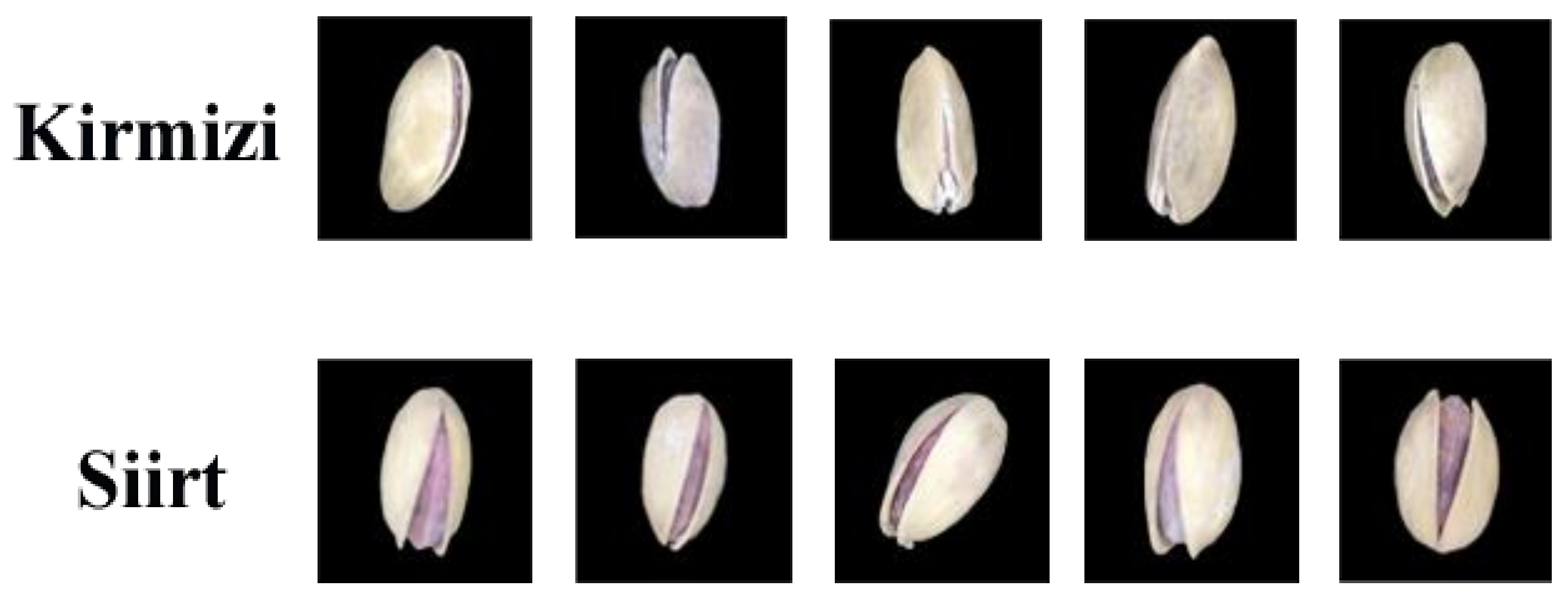
- Kirmizi and Siirt pistachio kernels were collected for this study. Each pistachio image was created by us for this study with a specially designed computer vision system.
- A dataset of 2148 images was obtained, with collected images of two pistachio types that are commonly grown.
- In order to determine the most suitable classification model, the most successful model was determined via classification performed by using different CNN architectures.
- A comprehensive analysis of CNN models was carried out and preliminary preparations were made for future studies.
2. Related Works
3. Materials and Methods
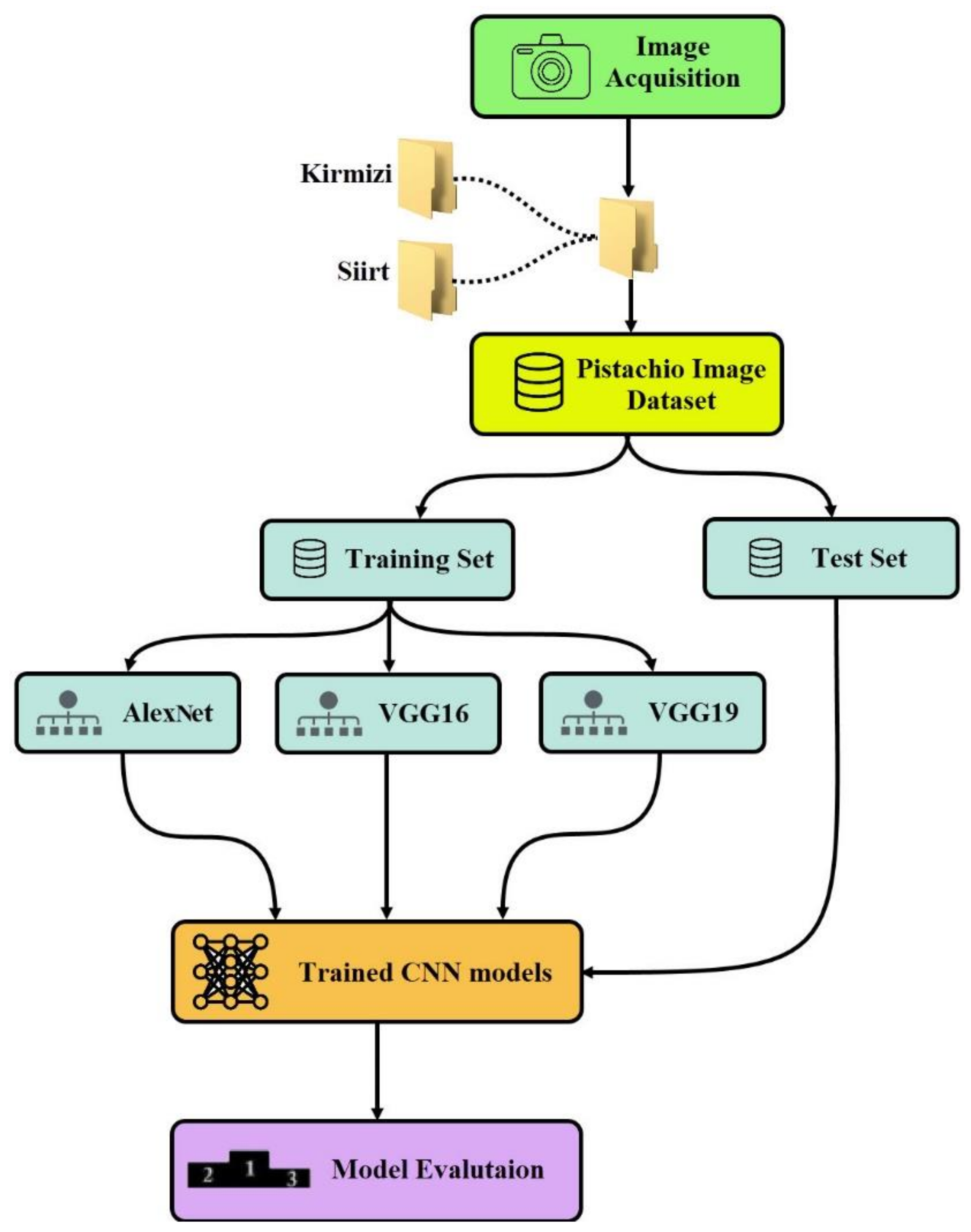
3.1. Image Acquisition
3.2. Pistachio Image Dataset
3.3. Convolutional Neural Network
3.4. Transfer Learning
3.5. Pre-Trained CNN Models
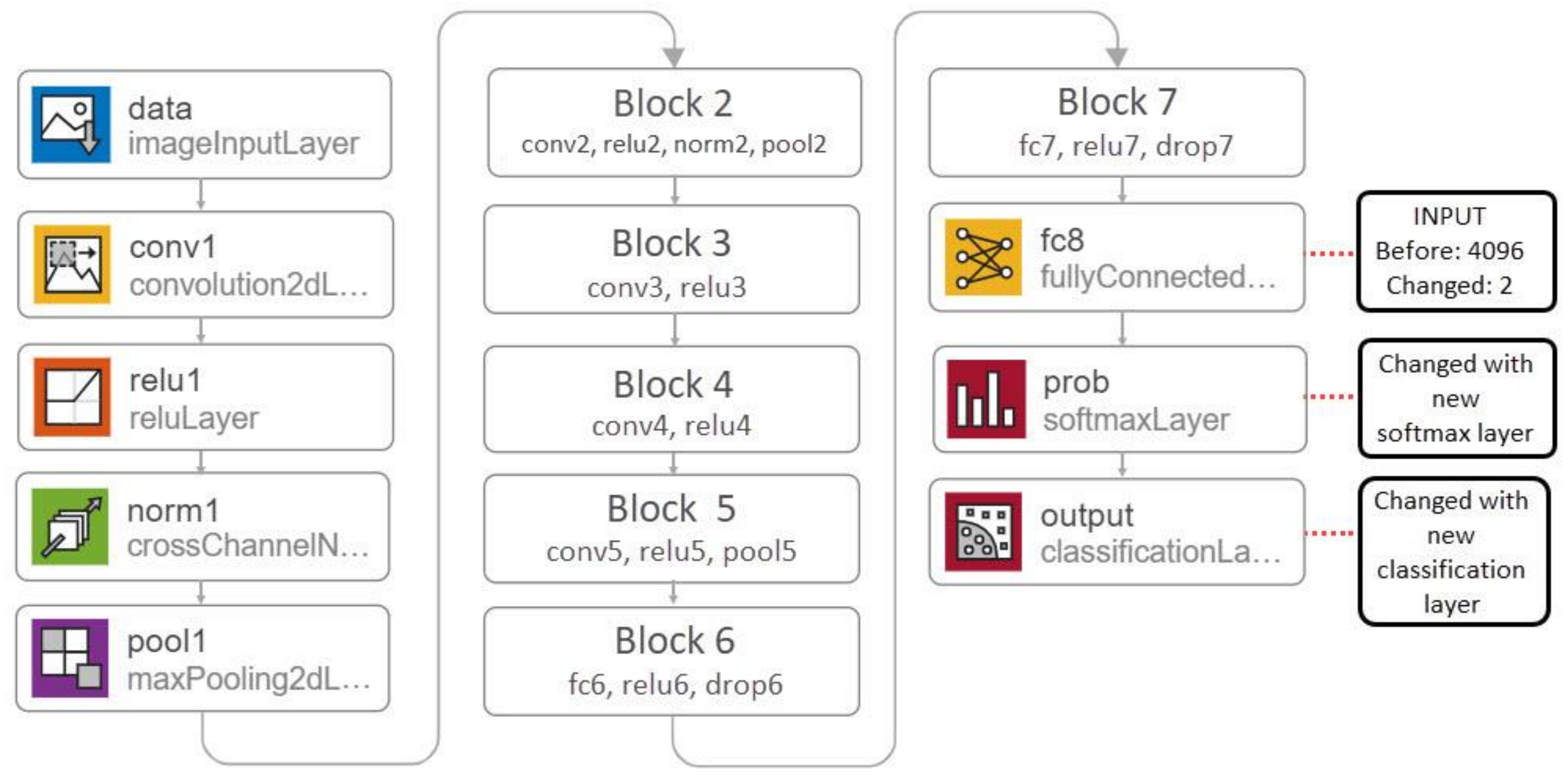
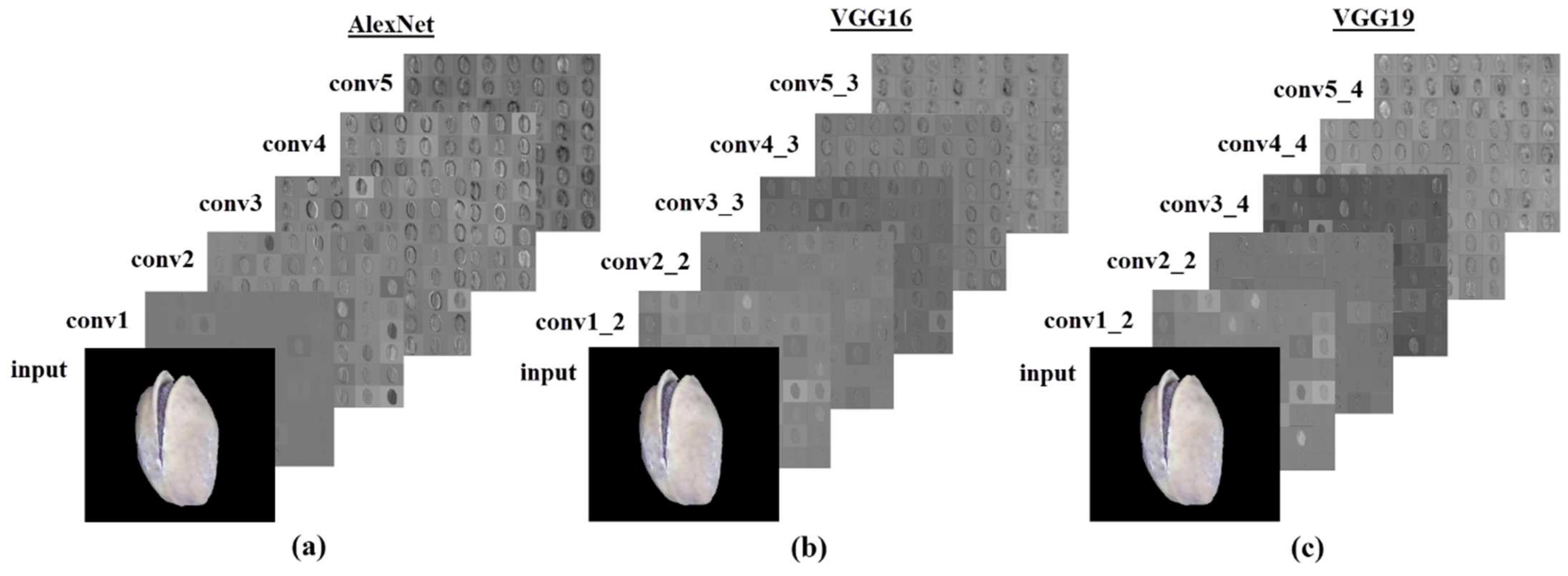
3.5.1. AlexNet
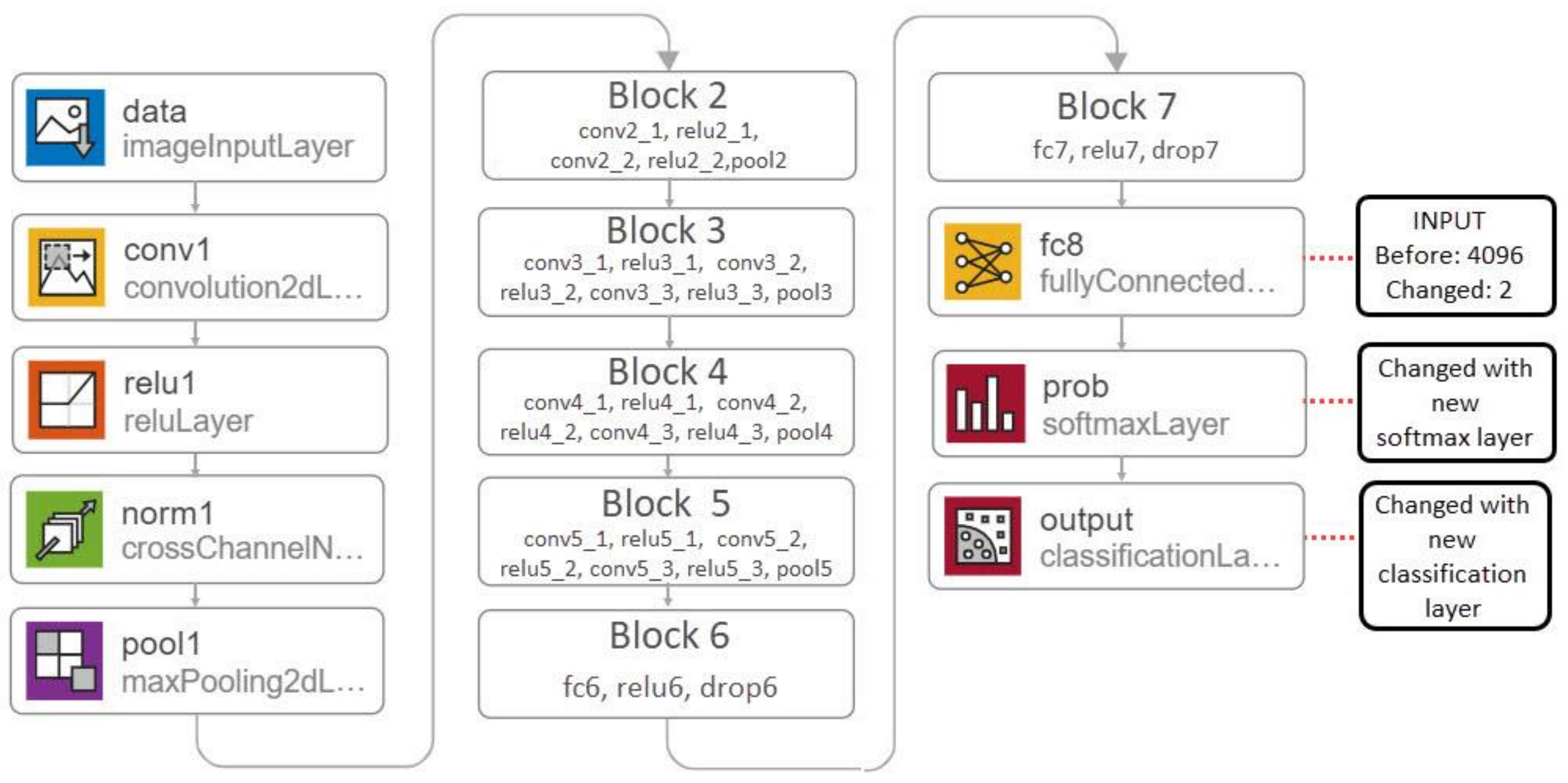
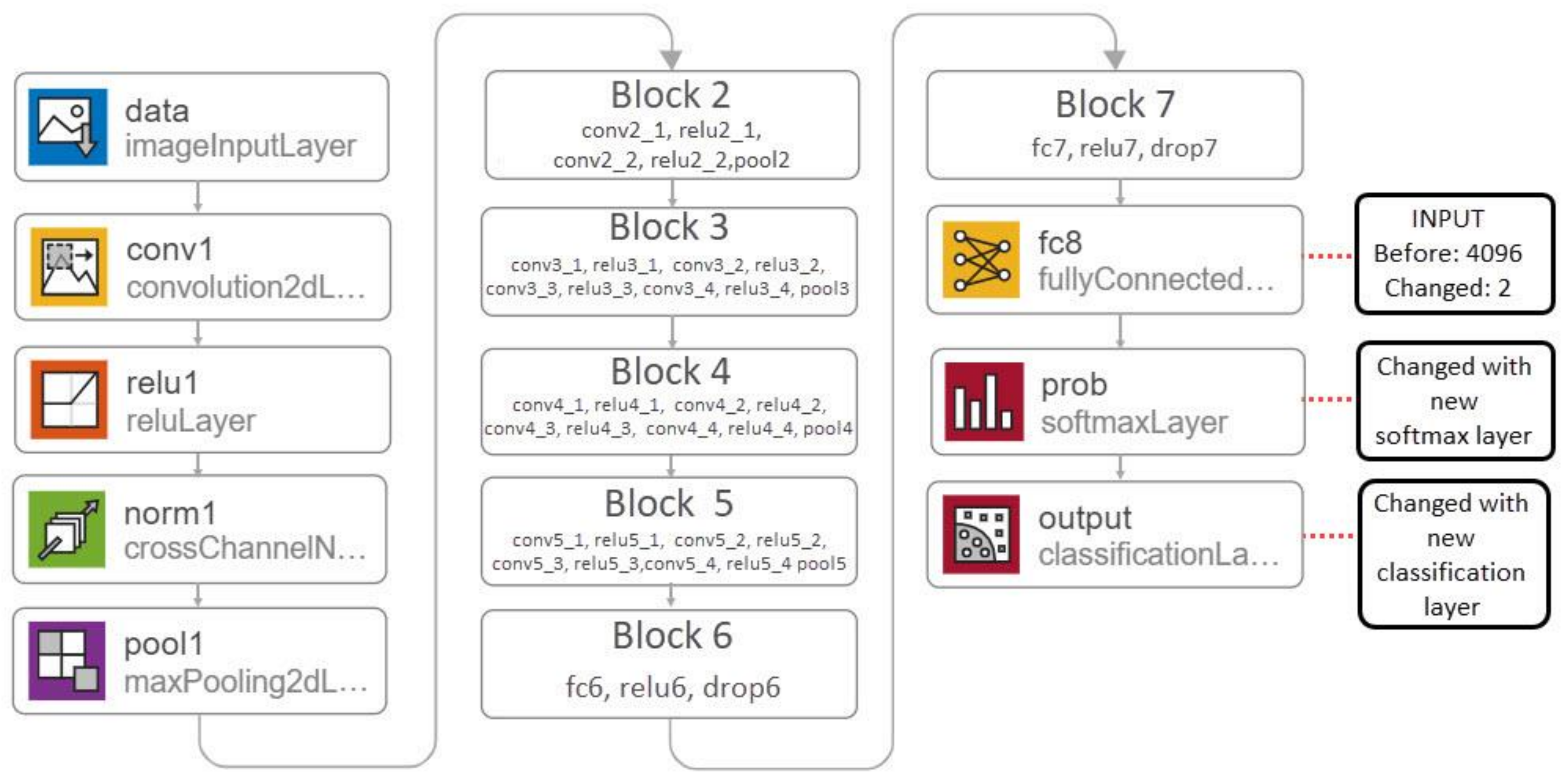
3.5.2. VGG16
3.5.3. VGG19
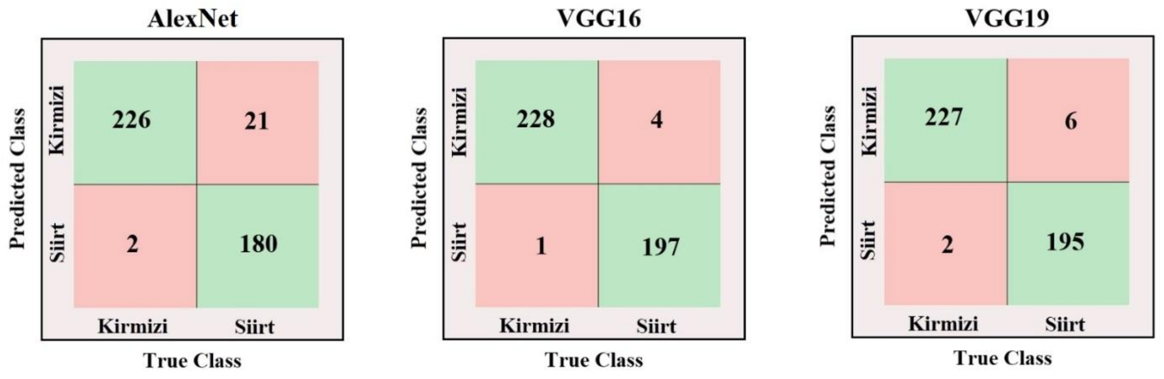
3.6. Confusion Matrix
- TP: True Positive. Examples where the true value of the model is 1 and the predicted value is 1.
- TN: True Negative. Examples where the true value of the model is 0 and the predicted value is 0.
- FP: False Positive. Examples where the true value of the model is 0 and the predicted value is 1.
- FN: False Negative. Examples where the true value of the model is 1 and the predicted value is 0.
3.7. Performance Metrics
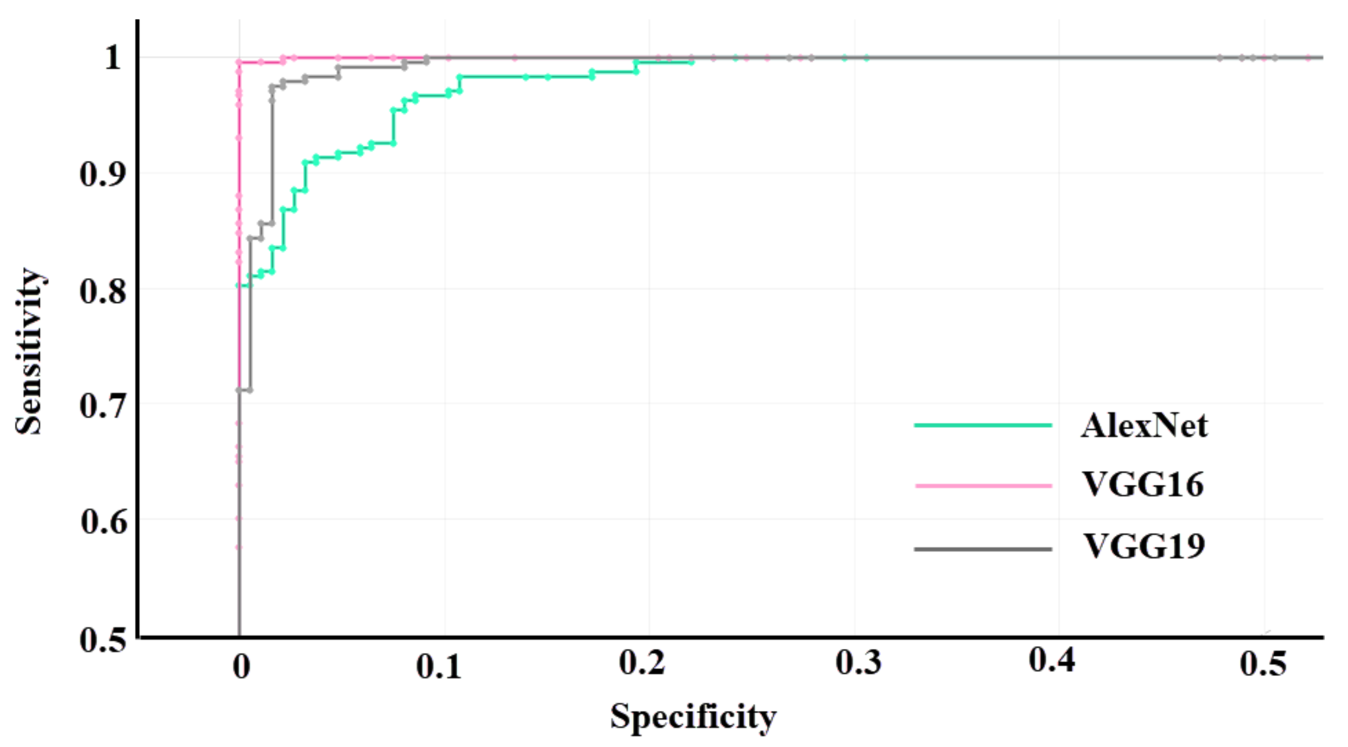
3.8. ROC and AUC
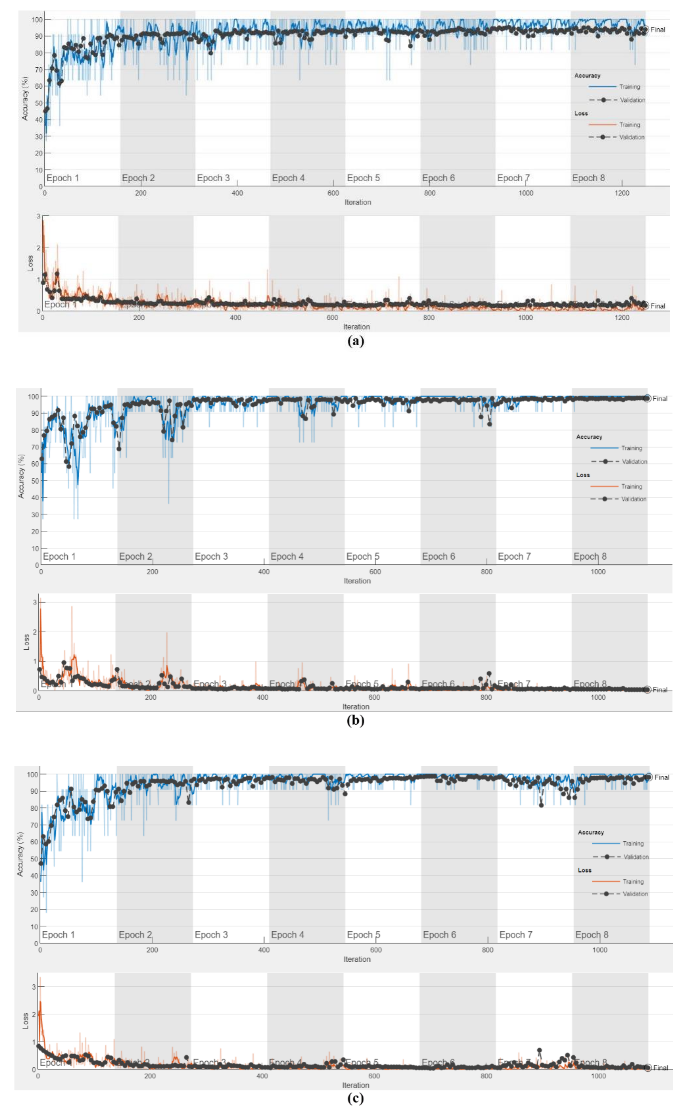
4. Experimental Results
5. Discussion and Conclusions
Author Contributions
Funding
Data Availability Statement
Conflicts of Interest
References
- Saglam, C.; Cetin, N. Prediction of Pistachio (Pistacia vera L.) Mass Based on Shape and Size Attributes by Using Machine Learning Algorithms. Food Anal. Methods 2022, 15, 739–750. [Google Scholar] [CrossRef]
- Parfitt, D.; Kafkas, S.; Batlle, I.; Vargas, F.J.; Kallsen, C.E. Pistachio. In Fruit Breeding; Springer: Berlin/Heidelberg, Germany, 2012; pp. 803–826. [Google Scholar] [CrossRef]
- Barghchi, M.; Alderson, P. Pistachio (Pistacia vera L.). In Trees II; Springer: Berlin/Heidelberg, Germany, 1989; pp. 68–98. [Google Scholar] [CrossRef]
- Kashaninejad, M.; Mortazavi, A.; Safekordi, A.; Tabil, L. Some physical properties of Pistachio (Pistacia vera L.) nut and its kernel. J. Food Eng. 2006, 72, 30–38. [Google Scholar] [CrossRef]
- Bonifazi, G.; Capobianco, G.; Gasbarrone, R.; Serranti, S. Contaminant detection in pistachio nuts by different classification methods applied to short-wave infrared hyperspectral images. Food Control 2021, 130, 108202. [Google Scholar] [CrossRef]
- Maskan, M.; Şükrü, K. Fatty acid oxidation of pistachio nuts stored under various atmospheric conditions and different temperatures. J. Sci. Food Agric. 1998, 77, 334–340. [Google Scholar] [CrossRef]
- Mahdavi-Jafari, S.; Salehinejad, H.; Talebi, S. A Pistachio Nuts Classification Technique: An ANN Based Signal Processing Scheme. In Proceedings of the 2008 International Conference on Computational Intelligence for Modelling Control & Automation, Vienna, Austria, 10–12 December 2008; IEEE: New York City, NY, USA, 2008. [Google Scholar] [CrossRef]
- Mahmoudi, A.; Omid, M.; Aghagolzadeh, A. Artificial neural network based separation system for classifying pistachio nuts varieties. In Proceedings of the International Conference on Innovations in Food and Bioprocess Technologies, Pathum Thani, Thailand, 12 December 2006. [Google Scholar]
- Khan, M.A.; Alqahtani, A.; Khan, A.; Alsubai, S.; Binbusayyis, A.; Ch, M.M.I.; Yong, H.-S.; Cha, J. Cucumber Leaf Diseases Recognition Using Multi Level Deep Entropy-ELM Feature Selection. Appl. Sci. 2022, 12, 593. [Google Scholar] [CrossRef]
- Yasmeen, U.; Khan, M.A.; Tariq, U.; Khan, J.A.; Yar, M.A.E.; Hanif, C.A.; Mey, S.; Nam, Y. Citrus Diseases Recognition Using Deep Improved Genetic Algorithm. Comput. Mater. Contin. 2021, 71, 3667–3684. [Google Scholar] [CrossRef]
- Shah, F.A.; Khan, M.A.; Sharif, M.; Tariq, U.; Khan, A.; Kadry, S.; Thinnukool, O. A Cascaded Design of Best Features Selection for Fruit Diseases Recognition. Comput. Mater. Contin. 2022, 70, 1491–1507. [Google Scholar] [CrossRef]
- Koklu, M.; Cinar, I.; Taspinar, Y.S. Classification of rice varieties with deep learning methods. Comput. Electron. Agric. 2021, 187, 106285. [Google Scholar] [CrossRef]
- Cinar, I.; Koklu, M. Classification of Rice Varieties Using Artificial Intelligence Methods. Int. J. Intell. Syst. Appl. Eng. 2019, 7, 188–194. [Google Scholar] [CrossRef] [Green Version]
- Farazi, M.; Abbas-Zadeh, M.J.; Moradi, H. A machine vision based pistachio sorting using transferred mid-level image representation of Convolutional Neural Network. In Proceedings of the 2017 10th Iranian Conference on Machine Vision and Image Processing (MVIP), Isfahan, Iran, 22–23 November 2017; IEEE: New York City, NY, USA, 2017. [Google Scholar] [CrossRef]
- Omid, M.; Firouz, M.S.; Nouri-Ahmadabadi, H.; Mohtasebi, S.S. Classification of peeled pistachio kernels using computer vision and color features. Eng. Agric. Environ. Food 2017, 10, 259–265. [Google Scholar] [CrossRef]
- Abbaszadeh, M.; Rahimifard, A.; Eftekhari, M.; Zadeh, H.G.; Fayazi, A.; Dini, A.; Danaeian, M. Deep Learning-Based Classification of the Defective Pistachios via Deep Autoencoder Neural Networks. arXiv 2019, arXiv:1906.11878. [Google Scholar]
- Dini, A.; Zadeh, H.G.; Rahimifard, A.; Fayazi, A.; Eftekhari, M.; Abbaszadeh, M. Designing a Hardware System to separate Defective Pistachios From Healthy Ones Using Deep Neural Networks. Iran. J. Biosyst. Eng. 2020, 51, 149–159. [Google Scholar] [CrossRef]
- Dheir, I.M.; Mettleq, A.S.A.; Elsharif, A.A. Nuts Types Classification Using Deep learning. Int. J. Acad. Inf. Syst. Res. 2020, 3, 12–17. [Google Scholar]
- Vidyarthi, S.K.; Tiwari, R.; Singh, S.K.; Xiao, H. Prediction of size and mass of pistachio kernels using random Forest machine learning. J. Food Process Eng. 2020, 43, e13473. [Google Scholar] [CrossRef]
- Rahimzadeh, M.; Attar, A. Detecting and counting pistachios based on deep learning. Iran J. Comput. Sci. 2021, 5, 69–81. [Google Scholar] [CrossRef]
- Ozkan, I.A.; Koklu, M.; Saraçoğlu, R. Classification of Pistachio Species Using Improved K-NN Classifier. Health 2021, 23, e2021044. [Google Scholar] [CrossRef]
- Krizhevsky, A.; Sutskever, I.; Hinton, G.E. ImageNet classification with deep convolutional neural networks. Commun. ACM 2017, 60, 84–90. [Google Scholar] [CrossRef]
- Dandıl, E.; Polattimur, R. Dog behavior recognition and tracking based on faster R-CNN. J. Fac. Eng. Archit. Gazi Univ. 2020, 35, 819–834. [Google Scholar] [CrossRef] [Green Version]
- Chen, H.; Chen, A.; Xu, L.; Xie, H.; Qiao, H.; Lin, Q.; Cai, K. A deep learning CNN architecture applied in smart near-infrared analysis of water pollution for agricultural irrigation resources. Agric. Water Manag. 2020, 240, 106303. [Google Scholar] [CrossRef]
- Arsa, D.M.S.; Susila, A.A.N.H. VGG16 in batik classification based on random forest. In Proceedings of the 2019 International Conference on Information Management and Technology (ICIMTech), Jakarta/Bali, Indonesia, 19–20 August 2019; IEEE: New York City, NY, USA, 2019. [Google Scholar] [CrossRef]
- Bayar, B.; Stamm, M.C. A deep learning approach to universal image manipulation detection using a new convolutional layer. In Proceedings of the 4th ACM Workshop on Information Hiding and Multimedia Security, Vigo, Spain, 20–22 June 2016. [Google Scholar]
- Glorot, X.; Bordes, A.; Bengio, Y. Deep sparse rectifier neural networks. In Proceedings of the Fourteenth International Conference on Artificial İntelligence and Statistics, Fort Lauderdale, FL, USA, 11–13 April 2011. [Google Scholar] [CrossRef]
- Akhtar, N.; Ragavendran, U. Interpretation of intelligence in CNN-pooling processes: A methodological survey. Neural Comput. Appl. 2020, 32, 879–898. [Google Scholar] [CrossRef]
- Habib, G.; Qureshi, S. Optimization and Acceleration of Convolutional Neural Networks: A Survey. J. King Saud Univ.-Comput. Inf. Sci. 2020. [Google Scholar] [CrossRef]
- Yosinski, J.; Clune, J.; Bengio, Y.; Lipson, H. How Transferable Are Features in Deep Neural Networks? arXiv 2014, arXiv:1411.1792. [Google Scholar]
- Kolar, Z.; Chen, H.; Luo, X. Transfer learning and deep convolutional neural networks for safety guardrail detection in 2D images. Autom. Constr. 2018, 89, 58–70. [Google Scholar] [CrossRef]
- Smirnov, E.A.; Timoshenko, D.M.; Andrianov, S.N. Comparison of regularization methods for imagenet classification with deep convolutional neural networks. Aasri Procedia 2014, 6, 89–94. [Google Scholar] [CrossRef]
- Sakib, S.; Ahmed, N.; Kabir, A.J.; Ahmed, H. An overview of convolutional neural network: Its architecture and applications. Preprints 2019, 2018110546. [Google Scholar] [CrossRef]
- Theckedath, D.; Sedamkar, R. Detecting affect states using VGG16, ResNet50 and SE-ResNet50 networks. SN Comput. Sci. 2020, 1, 1–7. [Google Scholar] [CrossRef] [Green Version]
- Koklu, M.; Cinar, I.; Taspinar, Y.S. CNN-based bi-directional and directional long-short term memory network for determination of face mask. Biomed. Signal Process. Control 2022, 71, 103216. [Google Scholar] [CrossRef]
- Carvalho, T.; de Rezende, E.R.S.; Alves, M.T.P.; Balieiro, F.K.C.; Sovat, R.B. Exposing Computer Generated Images by Eye’s Region Classification via Transfer Learning of VGG19 CNN. In Proceedings of the 2017 16th IEEE International Conference on Machine Learning and Applications (ICMLA), Cancun, Mexico, 18–21 December 2017; IEEE: New York City, NY, USA, 2017. [Google Scholar] [CrossRef]
- Simonyan, K.; Zisserman, A. Very deep convolutional networks for large-scale image recognition. arXiv 2014, arXiv:1409.1556. [Google Scholar]
- Tutuncu, K.; Cataltas, O.; Koklu, M. Occupancy detection through light, temperature, humidity and CO2 sensors using ANN. Int. J. Ind. Electron. Electr. Eng. 2016, 5, 63–67. [Google Scholar]
- Koklu, M.; Tutuncu, K. Classification of chronic kidney disease with most known data mining methods. Int. J. Adv. Sci. Eng. Technol. 2017, 5, 14–18. [Google Scholar]
- Acharya, U.R.; Fernandes, S.L.; WeiKoh, J.E.; Ciaccio, E.J.; Fabell, M.K.M.; Tanik, U.J.; Rajinikanth, V.; Yeong, C.H. Automated Detection of Alzheimer’s Disease Using Brain MRI Images—A Study with Various Feature Extraction Techniques. J. Med. Syst. 2019, 9, 302. [Google Scholar] [CrossRef] [PubMed]
- Rajinikanth, V.; Raj, A.N.J.; Thanaraj, K.P.; Naik, G.R. A Customized VGG19 Network with Concatenation of Deep and Handcrafted Features for Brain Tumor Detection. Appl. Sci. 2020, 10, 3429. [Google Scholar] [CrossRef]
- Koklu, M.; Kursun, R.; Taspinar, Y.S.; Cinar, I. Classification of Date Fruits into Genetic Varieties Using Image Analysis. Math. Probl. Eng. 2021, 2021, 4793293. [Google Scholar] [CrossRef]
- Taspinar, Y.S.; Cinar, I.; Koklu, M. Classification by a stacking model using CNN features for COVID-19 infection diagnosis. J. X-ray Sci. Technol. 2022, 30, 73–88. [Google Scholar] [CrossRef] [PubMed]

| No | Data Pieces | Class | Classifier | Accuracy (%) | References |
|---|---|---|---|---|---|
| 1 | 150 | 3 | ANN | 99.89 | Mahdavi-Jafari, Salehinejad, and Talebi (2008) |
| 2 | 1000 | 3 | AlexNet+SVM GoogleNet+SVM | 98 99 | Farazi, Abbas-Zadeh, and Moradi (2017) |
| 3 | 850 | 5 | ANN SVM | 99.40 99.80 | Omid et al. (2017) |
| 4 | 305 | 2 | Deep Auto-encoder Neural Networks | 80.30 | Abbaszadeh et al. (2019) |
| 5 | 958 | 2 | GoogleNet ResNet VGG16 | 95.80 97.20 95.83 | Dini et al. (2020) |
| 6 | 2868 | 5 | ConvNet | 98 | Dheir, Abu Mettleq, and Elsharif (2020) |
| 7 | 3927 | 2 | ResNet50 ResNet152 VGG16 | 85.28 85.19 83.32 | Rahimzadeh and Attar (2021) |
| 8 | 2148 | 2 | KNN | 94.18 | Ozkan, Koklu, and Saracoglu (2021) |
| True Class | |||
|---|---|---|---|
| Positive (P) | Negative (N) | ||
| Predicted Class | True (T) | TP | TN |
| False (F) | FP | FN | |
| Performance Metrics | Formulas |
|---|---|
| Accuracy | |
| F-1 Score | |
| Sensitivity | |
| Precision | |
| Specificity |
| AlexNet | VGG16 | VGG19 | |
|---|---|---|---|
| Elapsed Time | 17 min. 7 sec. | 90 min. 28 sec. | 99 min. 0 sec. |
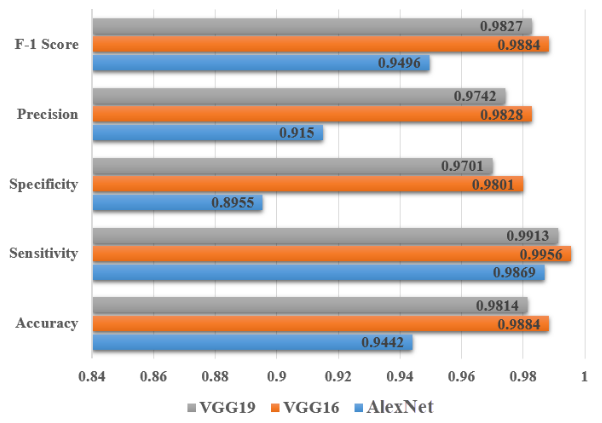
| AlexNet | VGG16 | VGG19 | |
|---|---|---|---|
| Accuracy | 0.9442 | 0.9884 | 0.9814 |
| Sensitivity | 0.9869 | 0.9956 | 0.9913 |
| Specificity | 0.8955 | 0.9801 | 0.9701 |
| Precision | 0.9150 | 0.9828 | 0.9742 |
| F-1 Score | 0.9496 | 0.9884 | 0.9827 |
| AlexNet | VGG16 | VGG19 | |
|---|---|---|---|
| Accuracy | 94.42 | 98.84 | 98.14 |
Publisher’s Note: MDPI stays neutral with regard to jurisdictional claims in published maps and institutional affiliations. |
© 2022 by the authors. Licensee MDPI, Basel, Switzerland. This article is an open access article distributed under the terms and conditions of the Creative Commons Attribution (CC BY) license (https://creativecommons.org/licenses/by/4.0/).
Share and Cite
Singh, D.; Taspinar, Y.S.; Kursun, R.; Cinar, I.; Koklu, M.; Ozkan, I.A.; Lee, H.-N. Classification and Analysis of Pistachio Species with Pre-Trained Deep Learning Models. Electronics 2022, 11, 981. https://doi.org/10.3390/electronics11070981
Singh D, Taspinar YS, Kursun R, Cinar I, Koklu M, Ozkan IA, Lee H-N. Classification and Analysis of Pistachio Species with Pre-Trained Deep Learning Models. Electronics. 2022; 11(7):981. https://doi.org/10.3390/electronics11070981
Chicago/Turabian StyleSingh, Dilbag, Yavuz Selim Taspinar, Ramazan Kursun, Ilkay Cinar, Murat Koklu, Ilker Ali Ozkan, and Heung-No Lee. 2022. "Classification and Analysis of Pistachio Species with Pre-Trained Deep Learning Models" Electronics 11, no. 7: 981. https://doi.org/10.3390/electronics11070981
APA StyleSingh, D., Taspinar, Y. S., Kursun, R., Cinar, I., Koklu, M., Ozkan, I. A., & Lee, H.-N. (2022). Classification and Analysis of Pistachio Species with Pre-Trained Deep Learning Models. Electronics, 11(7), 981. https://doi.org/10.3390/electronics11070981