Game-Theory-Based Multimode Routing Protocol for Internet of Things

Abstract

Various routing protocols have been proposed for ad hoc networks such as the Internet of Things (IoT). Most of the routing protocols introduced for IoT are specific to applications and networks. In the current literature, it is essential to configure all the network nodes with a single proposed protocol. Moreover, it is also possible for a single IoT network to consist of different kinds of nodes. Two or more IoT networks can also be connected to create a bigger heterogeneous network. Such networks may need various routing protocols with some gateway nodes installed. The role of gateway nodes should not be limited to the interconnection of different nodes. In this paper, a multi-mode hybrid routing mechanism is proposed that can be installed on all or a limited number of nodes in a heterogenous IoT network. The nodes configured with the proposed protocols are termed smart nodes. These nodes can be used to connect multiple IoT networks into one. Furthermore, a game-theory-based model is proposed that is used for intercommunication among the smart nodes to gain optimal efficiency. Various performance matrices are assessed under different network scenarios. The simulation results show that the proposed mechanism outperforms in broader heterogeneous IoT networks with diverse nodes.

1. Introduction

Various routing protocols for IoT have been proposed in the literature. Reactive, proactive, and hybrid methods are the most common [1]. In proactive routing, each node maintains an up-to-date routing table. To detect variations in the network, the nodes broadcast some control messages in the network. The reactive protocols are on demand: the source nodes generate some routing message whenever they need to send some data. Routing messages are flooded throughout the entire network. This mechanism is known as route discovery. When a path is determined, bandwidth is employed to communicate information [2]. Both protocols have advantages and disadvantages.

The type of network, features, and capabilities of nodes have a noteworthy effect on the efficiency or performance of various protocols. For example, nodes with higher mobility ratios outperform others when using the dynamic source routing (DSR) protocol [3]. According to this fact, we can assume that highly mobile nodes favor pure reactive protocols. Similarly, proactive protocols improve their packet delivery ratio (PDR) as the network size increases [4]. Additionally, proactive routing strategies result in fewer end-to-end delays. A hybrid of reactive and proactive protocols has been proposed by many researchers. Zone routing protocol (ZRP) [5] is the simplest basic hybrid protocol. The proactive routing is limited to the node’s immediate proximity in this routing protocol. The major goal is to reduce total network costs while taking into account the advantages and disadvantages of both types of reactive and proactive protocols.

Hybrid routing technologies combine reactive and proactive routing capabilities. The network is split into several sections in such protocols. The most typical option is to divide the network into zones or clusters [6]. If we partition a network into heterogeneous clusters or zones, there will be no use for the heterogeneity of member nodes within these segments. If we do not bind the nodes to a certain location, the heterogeneous routing protocols can be more efficient. Furthermore, the formation and frequent update of clusters, as well as the nomination of cluster heads (CHs), may result in additional node overhead [7]. Both clustered and non-clustered networks should be covered by the technique.

Multiple routing protocols can be used in the same network. In other words, by utilizing some gateway nodes, many different ad hoc networks can be merged into a single heterogeneous ad hoc network (HANETs). The basic goal of a larger network is to share and optimize resources [8]. Different nodes can use the help of other network nodes to get shorter pathways and transfer data to inaccessible nodes. The resourceful CHs are commonly regarded to be the gateway nodes [9]. Any programmable node should be assigned to the role of the gateway node. Furthermore, the role of gateway nodes in a heterogeneous network should not be confined to connecting distinct nodes. There should be a framework in place that allows gateway nodes to choose their own routing behavior. When choosing their routing behavior, nodes should take into account both their own parameters and the capabilities of the network. A node with proactive neighborhood, for instance, should adopt proactive routing. Similarly, in order to use less energy, nodes with lower remaining energies should switch to reactive routing. While communicating with other gateways and ordinary network nodes, gateway nodes should be able to intelligently choose a routing behavior.

Game theory (GT) is an economics and mathematics branch, but can be applied to any discipline to help people choose between several solutions. In the realm of networking, the GT technique is employed for a variety of objectives. Routing creation, application focus, network security, and network administration are the four fundamental factors that are used to model the relationship between wireless networks and GT [10]. The major goal of incorporating GT in wireless ad hoc networks is to construct a decision-making system in each node to enhance the performance of a network. To achieve improved throughputs, delays, energy consumption, and packet delivery ratios (PDR), GT is used to create routing algorithms for various types of ad hoc networks [9].

Smart nodes capable of understanding both reactive and proactive routing protocols are introduced in the proposed system. Such nodes will intelligently modify their routing behavior in response to network requirements and data traffic. These nodes serve as interfaces between nodes that have distinct routing protocols. By using such nodes, many heterogenous networks can be merged into a more efficient and larger network. The nodes in distinct networks with different routing protocols can be made to connect with each other to reduce delays in data transfer, boost dependability, and lessen energy usage. The routing protocol that will be used among the proposed smart nodes will also be studied and developed using a game-theoretic model. The smart nodes will be able to select the optimal routing protocol for their individual benefit and the benefit of the overall network.

The rest of the paper is organized as follows: The literature review is given in Section 2; Section 3 elaborates the proposed mechanism; the simulation results for different scenarios are given in Section 4; and lastly, in Section 5 the conclusion and future work are discussed.

2. Related Work

In ad hoc networks, GT can be used for a variety of purposes. GT has been used to create routing protocols for several types of ad hoc networks [10]. The major goal is to meet the QoS requirements. A ZRP-like GT-based protocol has been proposed by Selvi et al. [11]. In this mechanism, the node extinction rate is calculated to manage the network architecture. Moreover, to improve ad hoc QoS routing, a routing protocol based on the energy efficiency of zones is devised. This research describes a new way of enhancing the energy economy of ZRP-based protocols that control network topology by guessing node life expectancy. Furthermore, to increase QoS parameters, a game is paired with an efficient ZRP-based protocol. The authors state that the main objectives are to a) manage network topology according to the energy consumption rate; and b) improve QoS-aware techniques in terms of bandwidth, PDR, and some other parameters. Das and Tripathy [9] presented a technique that solely focuses HANETs. It focuses on cluster-based heterogeneous networks and comprises six phases. The GT model that is employed is a non-cooperative one. The basic goal is to construct clusters in a HANET as quickly as possible. The mixed strategies of several heterogeneous nodes are optimized using linear programming and GT.

A transmission power control-based strategy is described in the paper [12], which allows mobile nodes to balance transmission rate and power consumption to achieve a trade-off between transmission rate and power consumption. For each node, two tables define and update the average transmission rate as well as the amount of time the neighboring node is used for data transfer.

Some GT-based routing methods in ad hoc networks are primarily concerned with security. For device-to-device networks, Lv et al. [13] have suggested a secure GT-based routing algorithm. This proposed method operates in cluster-based networks. All data traffic is redirected through some secure routes that have been defined.

GT has been used by the authors to develop simple routing and load-balancing protocols. There is no mechanism in these strategies to handle diverse nodes in a wider network. The majority of GT-based routing methods place a premium on selfish node management. Zheng [14] proposes a reliable GT-based routing technique for a wireless sensor network (WSN) with certain selfish nodes. To balance resource consumption and reliability, a game model is applied. For resource-constrained network nodes, the network’s global information is not necessary. Furthermore, all nodes are free to act selfishly under this technique. Each player node’s four primary elements are taken into account in this proposed effort. This study takes into account transmission power, connectivity, dependability, and collision. Furthermore, network node heterogeneity is supported by the findings.

In recent years, a number of studies have been published proposing hybrid routing methods. The main focus of the majority of research projects has been on improving QoS parameters. The major goal is to improve targeted ad hoc networks by taking into account the following factors: latency, node energy, PDR, routing and processing overhead, and throughput [15]. ZRP [16] is a basic hybrid routing protocol that has been developed for many sorts of ad hoc networks. Various upgraded or modified variants of ZRP have been proposed in recent literature.

The “Dynamic Relationship-Zone Routing Protocol” (DRZRP) [17] is a ZRP-based protocol that focuses on relational zones rather than normal ZRP zones. The mechanism states that it is obvious for some nodes to communicate with non-zonal nodes on a regular basis. The zones, with a specified radius, are created based on the frequency of data transmission among the nodes. These zones are dynamically maintained, and the DRZRP algorithm decides proactive routing behavior inside these zones. This work is mainly concentrated on the delays and communication and processing overhead.

A sleep scheduling protocol based on ZRP has been proposed by Shanthy and Padma [18]. In this mechanism, the nodes are separated into zones and assigned to each zone with a zone leader. The selection of zone leader is based on residual energy, proximity, distance from the border, and link quality. To ensure load balancing, the zone leader detects many routes from border nodes to the target and distributes traffic along these channels. A sleep-duty cycling system that can be adjusted is also put in place. This is done so that energy is conserved at border nodes. The method is similar to other approaches that combine cluster-based processes with a sleep scheduling algorithm.

An enhanced ZRP protocol for vehicular ad hoc networks (VANETs) [19] has been proposed to efficiently meet diverse traffic circumstances. The zones are replaced with clusters in this technique, and some clustering mechanisms are used. The normal clustering mechanisms influence the majority of the work. Gasmi et al. [20] offer yet another modified ZRP. The writers of this study concentrate on the quality of service in the Internet of Vehicles (IoV). By utilizing the QoS function based on various parameters, a ZRP-based link-state mechanism is presented to improve IoV applications’ link stability.

For WSNs, the “State Aware Link Maintenance Approach” (SALMA) [15], a hybrid routing protocol, has been proposed. DSR and OLSR are used as the base protocols for the SALMA. There are three types of nodes: black, grey, and white. The classes are created based on the nodes’ activity status. During routing and data transfer, these various nodes use DSR, OLSR, or both protocols. This protocol was created specifically for WSNs and is therefore not useful in HANETs. In [21], several authors suggest that for MANETs, a dynamic cuckoo search (DCS) be combined with a hybrid zone-based hierarchical routing protocol (ZHRP). This mechanism focuses on improving interzone and intrazonal routing links.

Multimode routing protocols fall within the hybrid routing protocols category. These technologies make it simple for network nodes to switch between routing techniques. Different nodes in the same network may use different routing behaviors at the same time. Heo et al. [22] have suggested a hybrid routing system that allows nodes to vary their routing behavior. Each node in the network establishes its own routing protocol by examining several parameters at the start. The nodes do not change their routing protocols once they have been configured. Hoebeke and Demeester suggest another multimode routing scheme in their article [23]. Here, each node in the network has the ability to select a single routing mode and there are three primary modalities that are discussed: proactive, reactive, and flooding. The entireties in the routing table are also tagged with each node’s mode. A single routing database is used for all the network nodes. The base reactive and proactive protocols are AODV and WRP. This work does not address HANETs.

The authors in [24] propose a multipath heterogeneous ad hoc network “MHAR-OLSR” that combines MANET, FANET and VANET nodes. This multipath routing protocol uses a uniform communication language for heterogeneous ad hoc network components while taking into account their individual properties—transmission range, location, and speed. Four key components are the focus of this work: path classification, path computation, node identification and path selection. The TCMs are also modified in this work in order to achieve its objectives. Hauge et al. [25] outline an experiment with a depth first search (DFS) routing protocol that can be used as an inter-network routing protocol to establish a federated network that was conducted during the Coalition Warrior Interoperability eXercise (CWIX) 2019. The authors claim that their proposed work can be used in heterogeneous networks that have an interconnect overlay architecture. The authors also claim that this mechanism works very well with low-data-rate transmission technologies.

In [26], an autonomous cluster-based routing protocol is proposed. Some autonomous clusters are defined in heterogeneous MANETs. The proposed mechanism has the ability to efficiently route data in different domains. The gateways between different MANETs are designed to adaptively behave according to the nature of the data. Table 1 shows summary of relevant articles.

Table 1. Research papers focusing on game-theory-based routing.

Paper	Network and Focus	Summary
Das and Tripathy [9] (2019)	Heterogeneous Interconnectivity Clustering	▪ Non-cooperative game-theory-based routing protocol ▪ The clusters are made in six phases ▪ A single protocol is used throughout the heterogeneous network
Sharah et al. [12] (2021)	Homogeneous Transmission rate	▪ For network stability, a cooperative game is proposed ▪ The main objective is the load balancing among nodes ▪ For each neighbor, a single-hop transmission rate is used
Lv et al. [13] (2020)	Homogeneous Clustering Security	▪ Secure routing protocol based on clustering ▪ The packets are floated through some defined secure paths. ▪ No diversity of nodes or heterogeneity mentioned
Zheng [14] (2010)	Heterogeneous Selfish node	▪ Resource utilization based on a game-theory-based mechanism ▪ Each node independently acts as per its preferences ▪ The interconnectivity among heterogenous nodes is not discussed
Hu et al. [17] (2020)	Homogeneous Relational Zones	▪ Relationship-zones are proposed to replace the typical zones ▪ The nodes frequently communicating with each other are said to be part of a single zone. ▪ DRZRP protocol is used throughout the entire network
Shanthy and Padma [18] (2021)	Homogeneous Zones Work scheduling	▪ Similar to cluster-based mechanism ▪ A simple sleep scheduling mechanism is proposed ▪ Key parameters are energy level and degree of connectivity
Yang et al. [19] (2018)	Homogeneous Cluster	▪ Proposed for VANETs ▪ Clusters having similar functionalities to zones are proposed ▪ A cluster division and CH selection mechanism
Umar et al., 2016 [15]	Homogeneous Nodes’ states	▪ Uses OLSR and DSR as base protocols ▪ Nodes are classified according to their activity levels ▪ Each class of nodes has own routing procedure
Garmi et al. [20] (2020)	Homogeneous Link stability	▪ Mainly designed for Internet of Vehicles ▪ The foremost concern is the link stability ▪ A typical hybrid routing mechanism for homogeneous network
Gopalan [21] (2021)	Homogeneous Link stability	▪ Dynamic cuckoo search (DCS) () with hybrid zone hierarchical routing protocol (ZHRP)Interzonal and intrazonal link enhancement
Hoebeke et al. [23] (2012)	Homogeneous Multimode Routing	▪ Nodes can change from reactive to proactive or vice versa ▪ The nodes adapt their routing protocols in the beginning ▪ Three modes: reactive, proactive, and flooding are proposed
Benjbara et al. [24] (2022)	Heterogeneous Interconnectivity	▪ A modified version of OLSR is proposed ▪ The main objective is to combine MANETs, FANETs and VANETs ▪ The control messages of OLSR are modified to meet the diverse requirements of nodes
Hauge et al. [25]	Heterogeneous Interconnectivity	▪ A routing protocol based on depth first search ▪ Used to connect inter-networks during the Coalition Warrior Interoperability eXercise (CWIX) 2019 ▪ Also works well with low-data-rate transmission technologies
Okano et al. [26] 2015	Heterogeneous Interconnectivity	▪ An autonomous cluster-based routing protocol ▪ Capable of combining multiple MANETs ▪ The gateway nodes adaptively choose a routing behavior

3. Proposed Mechanism

The proposed study’s major goal is to design and create a network that uses many routing protocols to function together. In a single network, heterogeneity is measured in terms of distinct routing protocols. There may be nodes in a heterogeneous network with varying capabilities and parameters. Energy level, energy consumption ratio, mobility ratio, PDR, and so on are examples of these parameters. The nodes are meant to utilize a specific routing protocol based on the type of parameters.

Some intelligent nodes, known as smart nodes, are programmed to comprehend the routing behavior of various underlying heterogeneous nodes. By acting as gateways between the heterogeneous nodes, these nodes make it easier for them to communicate with one another. Furthermore, when these smart nodes communicate with one another, the most appropriate default routing behavior for them can be established to enhance the overall network’s performance. A game-theory based on the prisoner’s dilemma is used to change default routing behavior. This is an evolutionary process in which nodes evaluate the required parameters over time and adjust their routing behavior accordingly.

Two basic routing protocols are chosen to be employed to connect the nodes in the underlying ad hoc network. These protocols can be of any type. We generalize this by taking the two categories of reactive and proactive protocols. For communication, all the smart nodes can utilize one or both protocols. The preprogrammed nodes operate on a particular routing protocol and cannot be adapted. The smart nodes can include both routing characteristics. 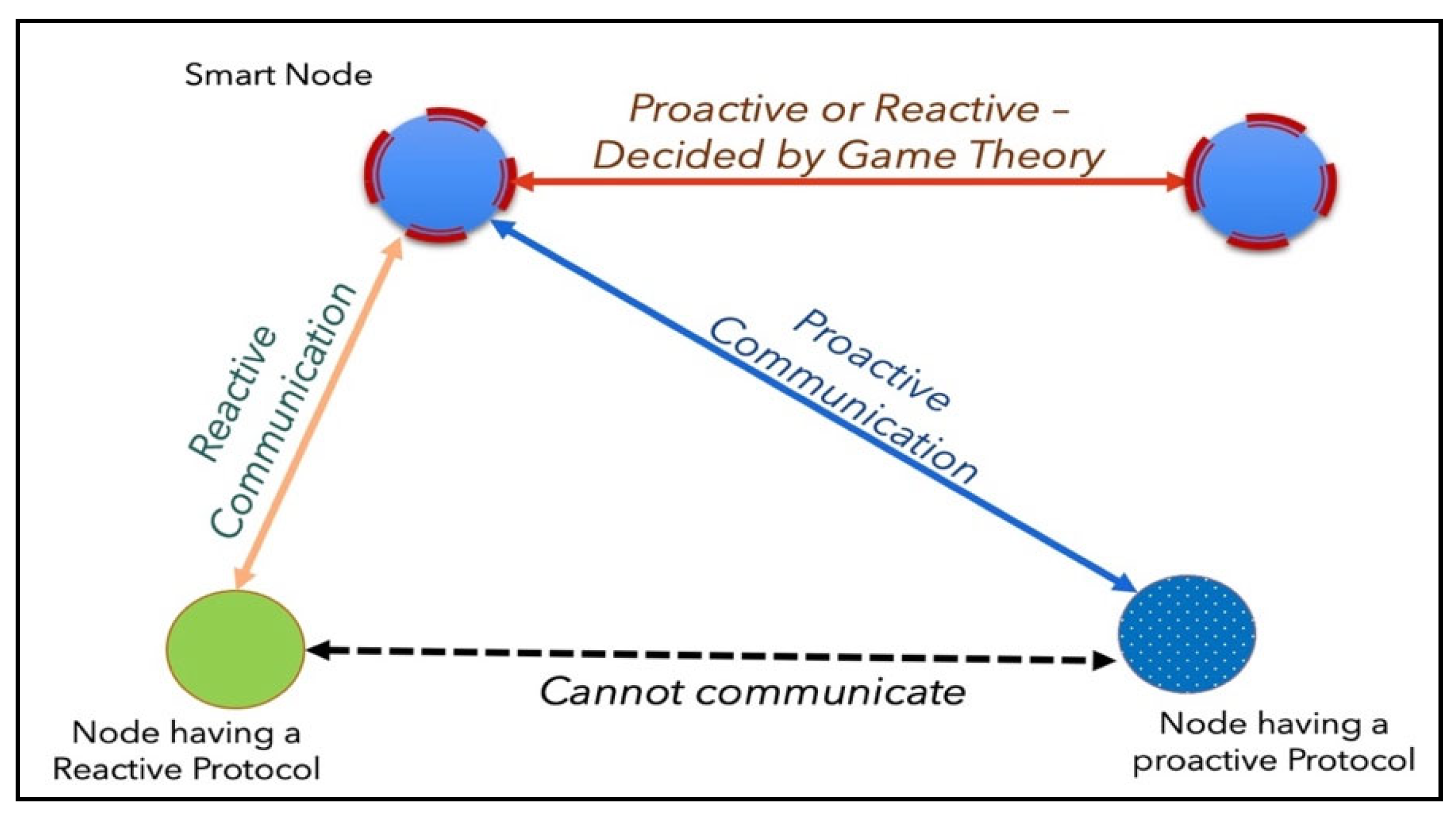Figure 1 depicts the three different classes of nodes. The nodes are classified based on their behavior. A HANET can be created by joining two or more networks that each have proactive and reactive nodes.

Figure 1. Proposed types of nodes and the in-between communication modes.

With the help of Figure 1, the routing capacity of smart nodes can be explained. In this diagram, a smart node communicates proactively with a proactive node while also being perceived as a member of its own family by a reactive node. Depending on their preferences and the GT, smart nodes adjust their routing behavior towards other smart nodes. A smart node can also operate as a connector between two separate nodes.

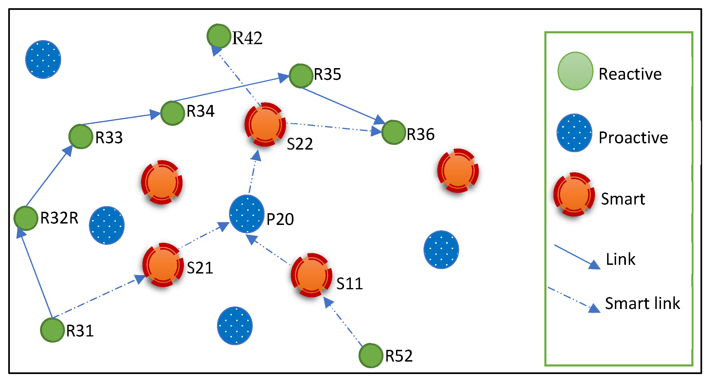
Figure 2 depicts a small network with heterogeneous nodes using three different routing strategies: proactive, reactive, and smart routing. There are five proactive and eight reactive nodes. This network could alternatively be thought of as a hybrid of two networks combined with the help of some smart nodes. Nodes with similar routing protocols may usually communicate with one another. The proposed smart routing technique, on the other hand, allows nodes with various routing protocols to communicate more effectively. The image depicts two sample scenarios, which are further detailed in Table 2:

Figure 2. Smart links interconnecting heterogeneous nodes.

Table 2. Two cases depicted in Figure 2.

Case #	Source	Destination	Intermediate Nodes
			With Smart Nodes	Without Smart Nodes
1	R31	R36	S21, P20, S22	R32, R33, R34, R35
2	R52	R42	S11, P20, S22	Not Accessible

We have two noteworthy cases, as shown in Figure 2 and Table 2. Both the source and destination nodes (R31 and R36) in the first scenario use a reactive routing protocol. A shorter route can be established by involving nodes from different classes when employing the proposed smart nodes. In case 2, two reactive nodes (R52 and R42) cannot connect to each other. These reactive nodes can be linked by enlisting the help of a proactive node and the proposed smart nodes.

This section is further broken into the following subsections: in Section 3.1, several sample network scenarios are given. Section 3.2 discusses the network’s key assumptions and characteristics. The game model is explained in Section 3.3, and the structure and actions of smart nodes are explained in Section 3.4.

3.1. Case Scenarios

While discussing the proposed mechanism, various possibilities might be considered. Figure 3, Figure 4, Figure 5 and Figure 6 depict several case scenarios.

Figure 3. Different nodes are positioned in distinct yet interconnected locations.

Figure 4. Dissimilar nodes are randomly deployed in the same area.

Figure 5. Nodes from the same class are deployed in an L form.

Figure 6. Most of the network nodes are smart nodes.

As demonstrated in Figure 3, two separate networks can be combined to form a larger heterogeneous network. The smart nodes allow the reactive and proactive nodes to connect with each other. Two kinds of communications in such types of heterogeneous networks are possible: common and unusual. In most cases, nodes send and receive data from other nodes that are comparable to them. Heterogeneous nodes communicate with each other in the situation of unusual communication. In this case, the proposed protocol’s performance for common type of communication may be inadequate. However, the suggested protocol outperforms when acting as a gateway between two different types of nodes for an unusual type of communication.

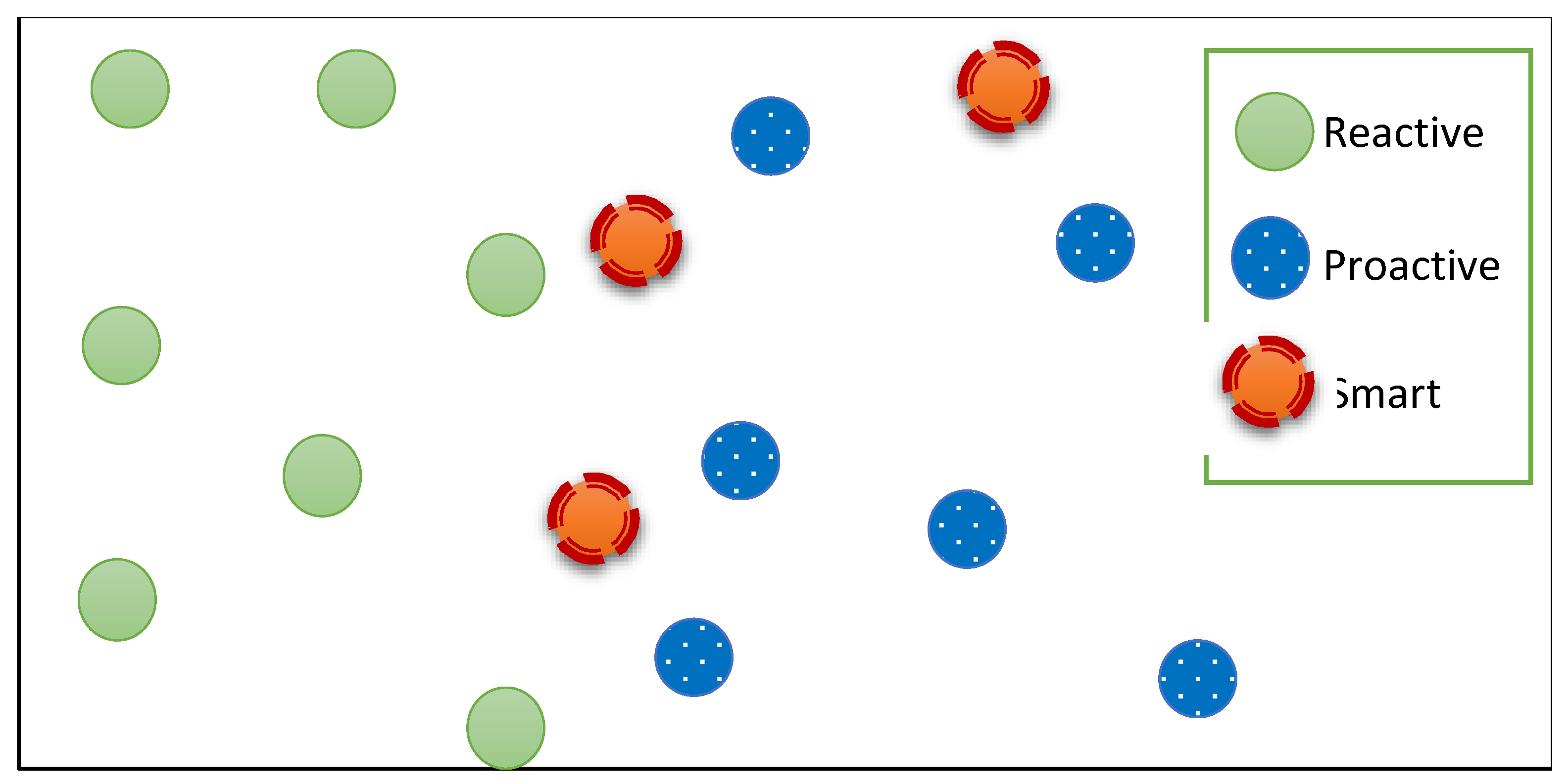
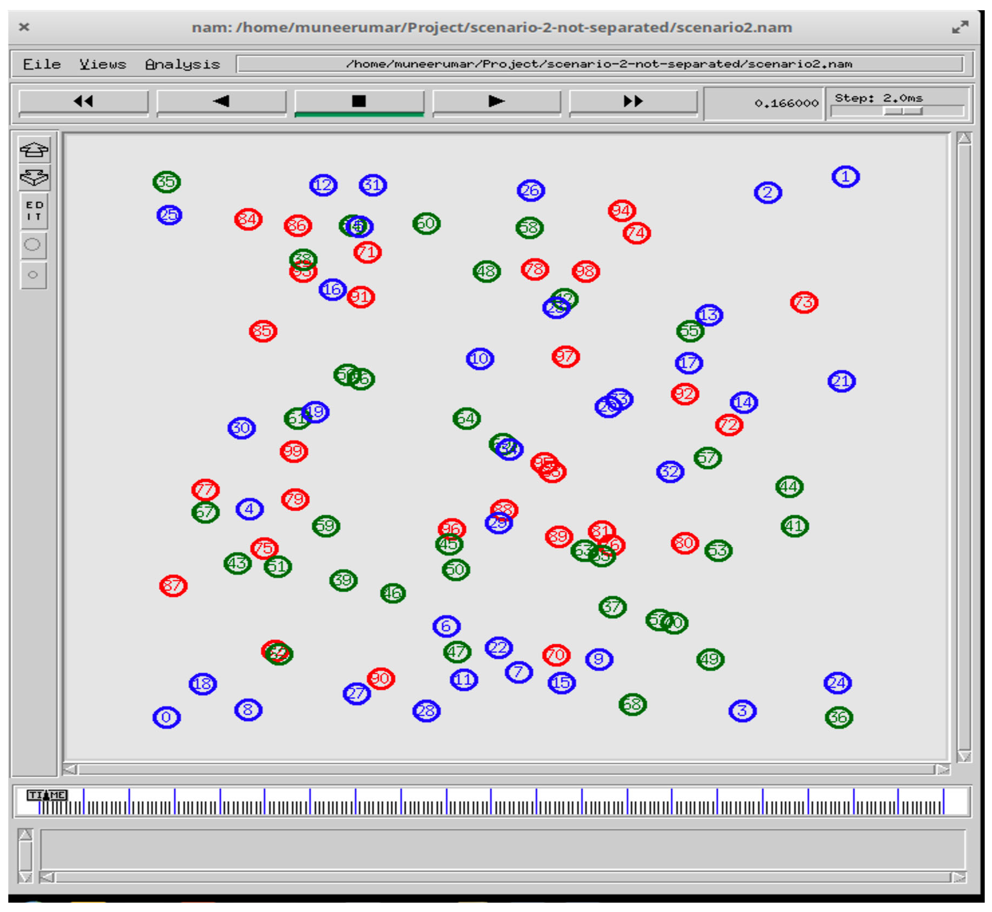
The different nodes in Figure 4 are distributed randomly in the same area. Both reactive and proactive nodes benefit from smart nodes, which allow them to more efficiently send and receive data.

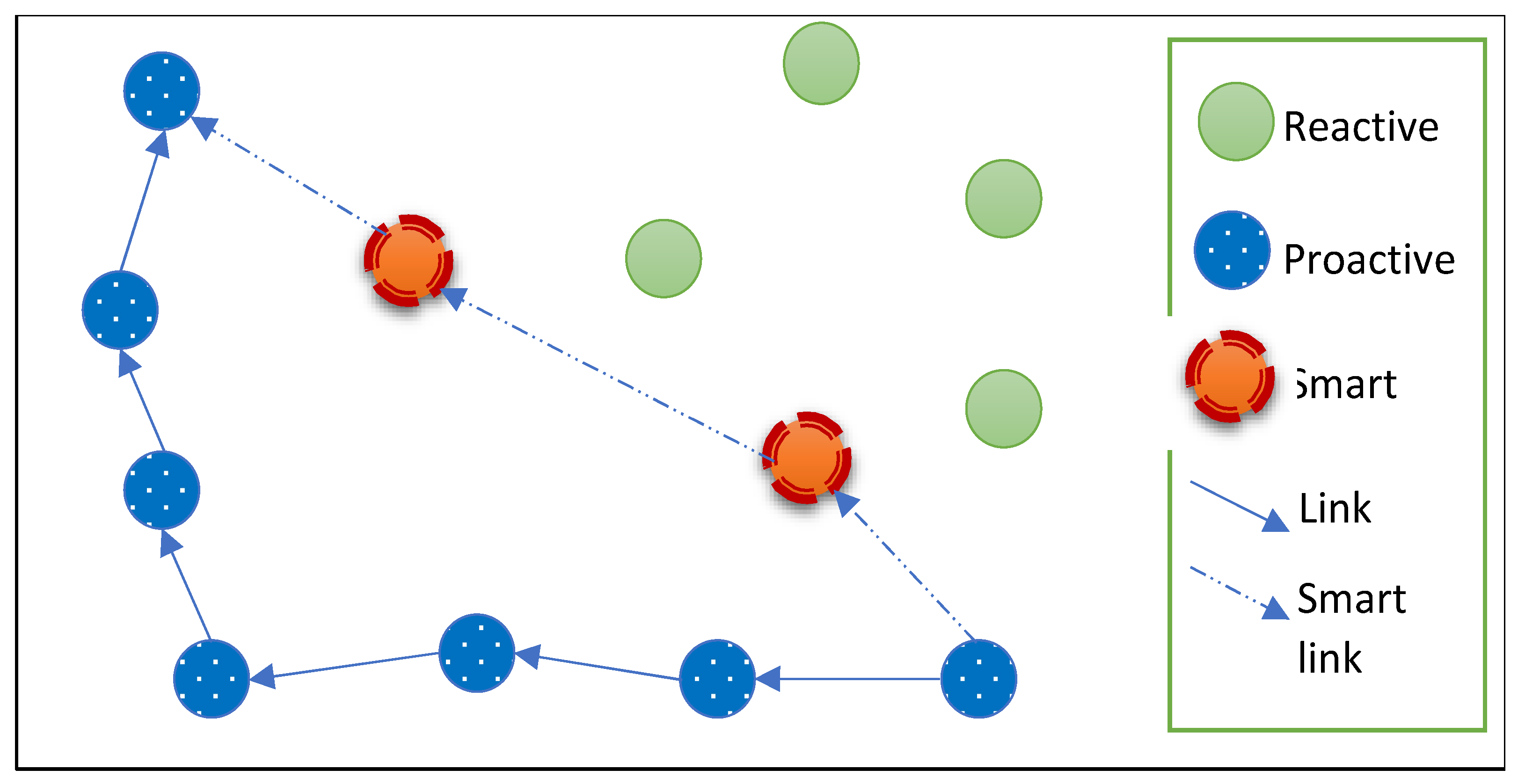
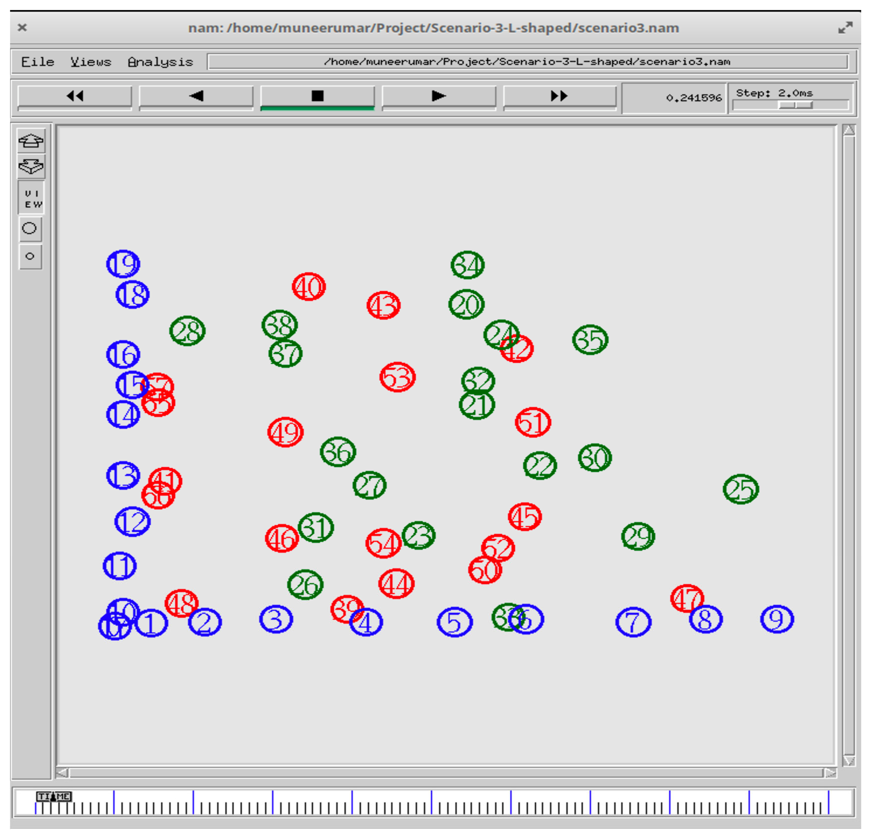
A case scenario is given in Figure 5, in which a class of nodes is arranged in an L form. If the top-most and the right-most nodes, from this class, want to communicate, they should follow the whole route through all the nodes of their class. Using smart nodes, a new diagonal route which is significantly shorter, can be created by involving nodes of another class. The smart link refers to a path that the smart nodes are involved in.

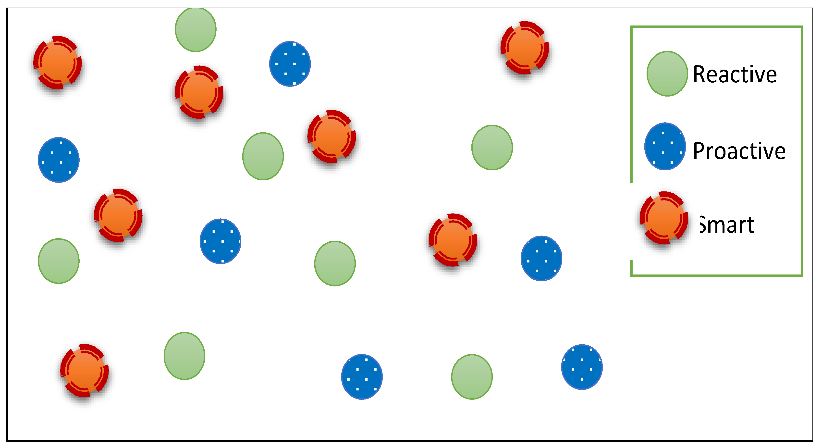
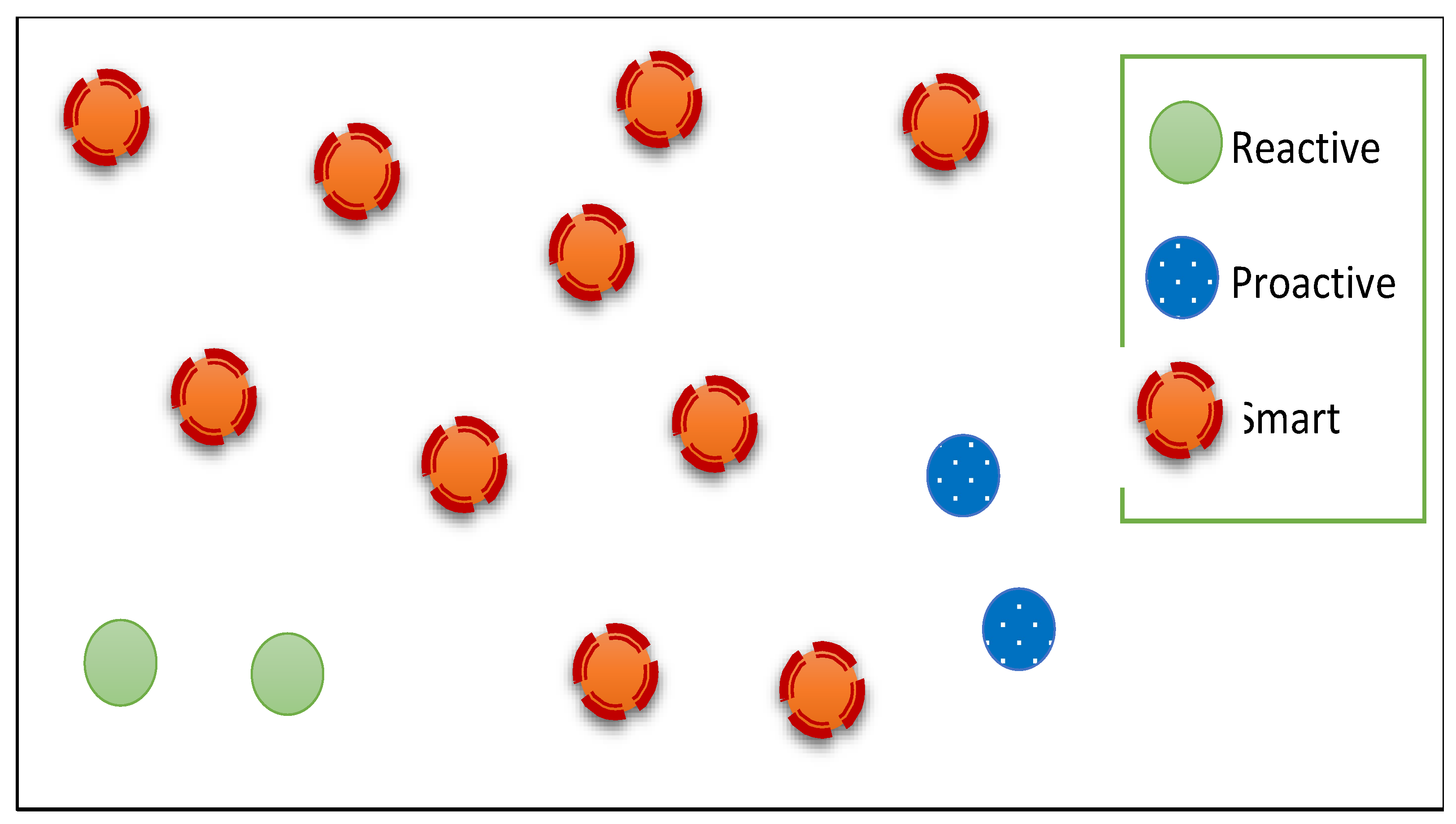
With the proposed smart nodes, a variety of options are available. As shown in Figure 6, a network made up of practically all of the smart nodes is achievable. In such a type of network, the nodes rationally adjust their routing behavior to be proactive or reactive. The adaptation relies on the node’s parameters first, then on the preferences of all known nodes.

3.2. Assumptions and Features

The following are the essential assumptions and aspects of the proposed mechanism:

3.2.1. Network Model

The network is assumed to have a variety of nodes. The network can be compared to a game denoted by G as shown in Equation (1). Where $N$ represents the set of all the nodes of heterogeneous connected networks, $S$ denotes the strategies, and $U$ and $I$ are used for utility and improvement functions, respectively.

$$G=\left[ N, S,U, I \right]$$

(1)

3.2.2. Network Layer

At the physical layer, all nodes are believed to have the same attributes. Only at the network layer do the heterogeneous nodes use distinct routing behaviors. If we suppose that there is also heterogeneity at the physical layer, then the proposed smart nodes should be able to decode the various signals sent by heterogeneous nodes. The smart nodes could use a variety of physical interfaces to understand different signals. However, this work focuses mainly on the network layer.

3.2.3. Base Protocols

The network uses two base protocols: AODV and DSDV. AODV is a reactive protocol, whereas the latter is proactive. Any of these protocols can be used by any of the network nodes. The smart nodes can understand both protocols, but only one of them is used for communication at a time. Other protocols instead of AODV and DSDV can also be used in the proposed mechanism. However, our main focus is on these two protocols during the design and implementation.

3.2.4. Classifications of Nodes

Two groups of nodes can be made based on two classes: type of nodes and protocol-based nodes. There are four types of nodes in the node-type category: (a) source, (b) destination, (c) relay, and (d) neighbor nodes. Equations (2)–(5) are used to define these four types.

$$Sn\in N : \left\{n_i\in N_{alive}\wedge n_i\in N_{adi}\right\}$$

(2)

The source node is denoted by $Sn$ that is the node $n_i$ member of network N. $Sn$ is a member of alive nodes $N_{alive}$ and active data initiating nodes $N_{adi}$.

$$Dn\in N : ni\in Nalive\wedge ni\in Nadr Dn\in N : \left\{n_i\in N_{alive}\wedge n_i\in N_{adr}\right\}$$

(3)

In Equation (3), $Dn$ denotes the destination nodes that are members of sets of alive and active data receiver nodes $N_{adr}$.

$$NEn\in N : \left\{n_j\in RtTbl{e}_{\mathrm{i}}\wedge n_j is NextHop\right\}$$

(4)

The set of neighbor nodes of node $n_i$ can be represented by $NEn$. $NE{n}_j$ is a neighbor node of $n_i$ that is present in the routing table $RtTble$ of node $n_i$, and is marked as $NextHop$.

$$REn\in N : \left\{n_i\in N_{alive}\wedge n_i\in N_{adf}\wedge n_i\in RtTbl{e}_{Sn}\right\}$$

(5)

In Equation (5), a relay node $RE{n}_i$ is the node that is present in the routing table of source node $Sn$.

Different classes of routing protocols can be used for network nodes. Each node must belong to at least one class as shown in Equation (6). The entire heterogeneous network is composed of the nodes belonging to these classes.

$$N=\left\{n_{i }\in ClassA \vee n_{i }\in ClassB \vee n_{i }\in ClassC\dots \right\}$$

(6)

In our case, we are using three classes: $ClassA$ for proactive nodes, $ClassB$ for reactive nodes, and $ClassC$ for smart nodes. In the proposed mechanism the three classes can be further defined by Equations (7)–(9).

$$ProN\in N:\left\{n_{i }\in ClassB | Generates TCM \cup Responds to TCM\right\}$$

(7)

The proactive nodes, $ProN$ belonging to $ClassB$, periodically generate topological control messages (TCM) also known as HELLO messages. These nodes also respond to relevant TCM.

$$ReaN\in N:\left\{n_{i }\in Class\mathrm{B} | Generates RPkt \cup Responds to RPkt\right\}$$

(8)

$ReaN$ denote the reactive nodes. These nodes belong to $ClassB$. These nodes generate and receive routing packets i.e., route request (RREQ), route replies (RREP), and route errors (RERR).

$$SmrtN\in N:\left\{n_{i }\in ClassC | ClassC=ClassA \cap ClassB\right\}$$

(9)

Both reactive and proactive features are present in smart nodes $SmrtN$. These nodes represent the coming together of reactive and proactive activities.

3.2.5. Neighborhood and Routing Tables

Routing tables are available in two different formats. The routing table used by $ClassA$ nodes is shown in Table 3.

Table 3. Routing table for ClassA (Proactive).

Destination IP

Next Hop

Metric

Dest. Seq. Number

$ClassB$ nodes retain routing information in their routing tables in the following format shown in Table 4.

Table 4. Routing Table for ClassB (Reactive).

Destination IP

Seq. #

Hop-Count

Next Hop

Validity Time

For the storage of routing information, a $SmrtN$ uses both $ClassA$ and $ClassB$ routing tables. A translator is kept in such nodes to change the values between both the routing tables. Furthermore, each smart node maintains an additional table in which it stores information about its neighbors. These data are gathered after a certain amount of time has passed in order to compute the data about neighbor nodes. The table primarily comprises energy and consumption ratios, and neighbors’ mobility ratios as shown in Table 5.

Table 5. Information about Neighbors.

Neighbor-ID

Remaining-Energy

Energy-Consump.-Ratio

Mobility-Ratio

3.2.6. Nodes’ Energy Level

Each node has a finite amount of energy. Due to their heterogeneous nature, nodes’ energy levels may differ from one another. If a node has enough energy to be spent on data packet transmission, processing, and reception, it is said to be alive. The dead nodes cannot be considered as part of the network. At any point in time if a node fails due to any reason—such as breakage or battery failure—then the node can be considered a dead node.

$E\left(n_i\right)$ and $E_{Initial}\left(n_i\right)$ are the current and initial energies of a node $n_i$, respectively. The ratio of a node’s energy consumption over time $t$ is defined as, $\Delta E^t\left(n_{i }\right)=E^{T-t}\left(n_{i }\right)-E^T\left(n_{i }\right)$. After a certain amount of time, the energy fluctuation must fulfill the equation $E\left(n_i\right)>\Delta E\left(n_i\right)$. The value $\Delta E$ may differ for each node due to the heterogeneous environment. $E_{Rmn}^t\left(n_i\right)$ is the remaining energy ratio of a node, $n_i$ at time $t$, as computed in Equation (10).

$$E_{Rmn}^t\left(n_i\right)=\frac{E^t\left(n_i\right)}{E_{Initial}\left(n_i\right)}$$

(10)

In Equation (11), $\lambda E^t\left(n_{i }\right)$ represents the current energy to energy consumption ratio at time $t$ of a node $n_i$.

$$\lambda E^t\left(n_i\right)=\frac{E^t\left(n_i\right)}{\Delta E^t\left(n_i\right)}$$

(11)

The median of the known nodes’ $\lambda E^t\left(n_j\right)$ can be used to calculate the energy threshold value, $ThE$, as shown in Equation (11). Each smart node can send a request to its known nodes to get these values.

$$ThE=Med\left(\lambda E^t\left(n_j\right)\right)$$

(12)

3.2.7. Nodes’ Mobility Ratio

The network’s nodes are mobile and have variable mobility ratios. The kth location of a node $n_i$ is $Lo{c}_k\left(n_i\right)=\left(x_k,y_k\right)$ where $x$ and $y$ are the coordinates. If a node $n_i$ moves from location k to location l in a time period t, then it can be denoted as $\Delta Lo{c}_{k,l}^t\left(n_i\right)$ and computed as in Equation (12).

$$\Delta Lo{c}_{k,l}^t\left(n_i\right)=\frac{\sqrt{{\left(x_k-x_l\right)}^2+{\left(y_k-y_l\right)}^2}}{t}$$

(13)

The same can be said for the $n_i$ node’s mobility ratio, which is indicated by $MobRatio(n_i)$. A smart node requires a threshold value for mobility ratio, $ThM$, during default protocol selection, which can be calculated using Equation (13).

$$ThM=Med\left(MobRatio\left(n_j\right)\right)$$

(14)

3.3. Game Modeling

As previously stated, the network can be viewed as a game. The strategies and utility functions of player nodes as well as the game matrix and improvement functions are addressed in this subsection.

3.3.1. Nodes’ Strategies and Utility Function

S denotes the strategy of nodes towards routing protocol selection in the game. The routing behavior of a node is determined by three major characteristics. The energy level, consumption ratio, and mobility ratio of the nodes are these metrics. A proactive routing technique is preferred by nodes with a higher degree of energy while highly mobile nodes, on the other hand, require reactive routing for best results.

The nodes first examine their mobility ratio. For a higher value of mobility, the nodes adjust their default routing protocol to reactive. If the mobility level is higher, then the energy consumption ratio and current level are examined. With the reduced energy consumption ratio, nodes with a higher energy level adapt to proactive routing behaviour. A node’s power is tested afterward. For a smart node $n_i$, i.e., $SmrtN\in$ N, two strategies are defined: $S_i=\left\{s_r,s_p\right\}$, where $s_r$ represents the strategy with a reactive protocol ($ReaN$) and $S_i=s_p$ denotes a member of the $ProN$ class, i.e., proactive node. If two smart nodes with different routing protocols are communicating with each other, then an adequate level of energy and time is wasted on unwanted routing and topology control packets. This wastage can be considered the transmission cost on routing. The payoff functions are determined by node strategies. Equation (14) can be used to define the payoff function for two smart nodes.

$$U\left(n_i,n_j\right)=\left\{\begin{array}{c}\frac{1}{C_{ProN,i}},\frac{1}{C_{ReaN,j}} where RP\left(n_i\right)\ne RP\left(n_j\right)\\ \left(1,1\right) where RP\left(n_i\right)=RP\left(n_j\right)\end{array}\right.$$

(15)

where $C_{ProN,i}$ is the cost of routing for the class of proactive nodes due to the smart node $n_i$. Between two smart nodes, the following game matrix can be formed:

There is no need to change the routing protocol of $n_{i }$ and $n_j$, if both are using the same routing protocol. If two nodes have distinct routing behaviors, their routing performance will be impaired, as shown in the Table 6. The situation where both the smart nodes operate on different protocols is referred to as the degraded protocols and denoted by Δ R and Δ P. It is clear from Lemma 1 that the game strageies form a pure Nash Equilibrium.

Table 6. Game matrix.

		Node j
		Proactive (S = s2)	Reactive (S = s1)
Node i	Proactive $(S=s_p$)	$\left(1, 1\right)$	$\frac{1}{C_{ReaN,i}},\frac{1}{C_{ProN,j}}$
	Reactive $(S=s_r$)	$\frac{1}{C_{ProN,i}},\frac{1}{C_{ReaN,j}}$	$\left(1, 1\right)$

Lemma1. 

In the proposed game, the strategy pairs$\left(s_r,s_p\right)$and$(s_p,s_r$) form a pure Nash Equilibrium.

Proof. 

There are two major classes of nodes in the network. These are reactive and proactive classes. Each smart node is allowed to choose either of these two routing protocols. In Table 5 the strategies are given along with the payoffs. In case both the interacting nodes use the same routing protocol then there will be an optimal situation denoted by $\left(1, 1\right)$. It is clear that the payoff should be less than 1 for the cases $\left(s_r,s_p\right)$ and $(s_p,s_r$). The distinct nodes should change their strategies to gain an optimal payoff. Therefore, according to the definition, the situation is a pure Nash Equilibrium for this game. □

To switch the routing from a costly routing protocol, an evolutionary technique, referred to as the improvement function $I$, is used.

3.3.2. Improvement Function

Each node in the network establishes its default routing protocol at the outset and refreshes it after a certain amount of time has passed. With the passage of time, the default behavior changes based on the parameters considered. If a node in the game matrix receives Δ R or Δ P. It kicks off the game’s second phase. Both of its routing tables are scanned. The NextHop fields are checked in both tables. Using the following Equation (15), to obtain the most common routing protocol in the neighborhood, the entries are counted and compared.

$$Count Distinct\left(Pr{o}_{RtTbl{e}_{NextHop}}\right)>Count Distant\left(Re{a}_{RtTbl{e}_{NextHop}}\right)$$

(16)

If the criterion is met, the node $n_i$ adjusts to proactive as its default routing protocol; otherwise, it switches to reactive protocol. If the node receives Δ R or Δ P again, it evaluates all of the stored nodes in its routing tables, and accordingly modifies its routing protocol, following the same approach as with Equations (16)–(18).

$$Tota{l}_{Pro}=Distinct\left(Pr{o}_{RtTbl{e}_{All nodes}}\right)$$

(17)

$$Tota{l}_{Rea}=Distinct\left(Re{a}_{RtTbl{e}_{All nodes}}\right)$$

(18)

$$SizeOf\left(Tota{l}_{Rea}\right)>SizeOf\left(Tota{l}_{Pro}\right)$$

(19)

Two sets, $Tota{l}_{Rea}$ and $Tota{l}_{Pro}$, are used in these equations and are known to node $n_{i }$. The node $n_{i }$ switches its routing behavior according to the largest known routing protocol in the network.

3.4. Architecture and Functions of Smart Nodes

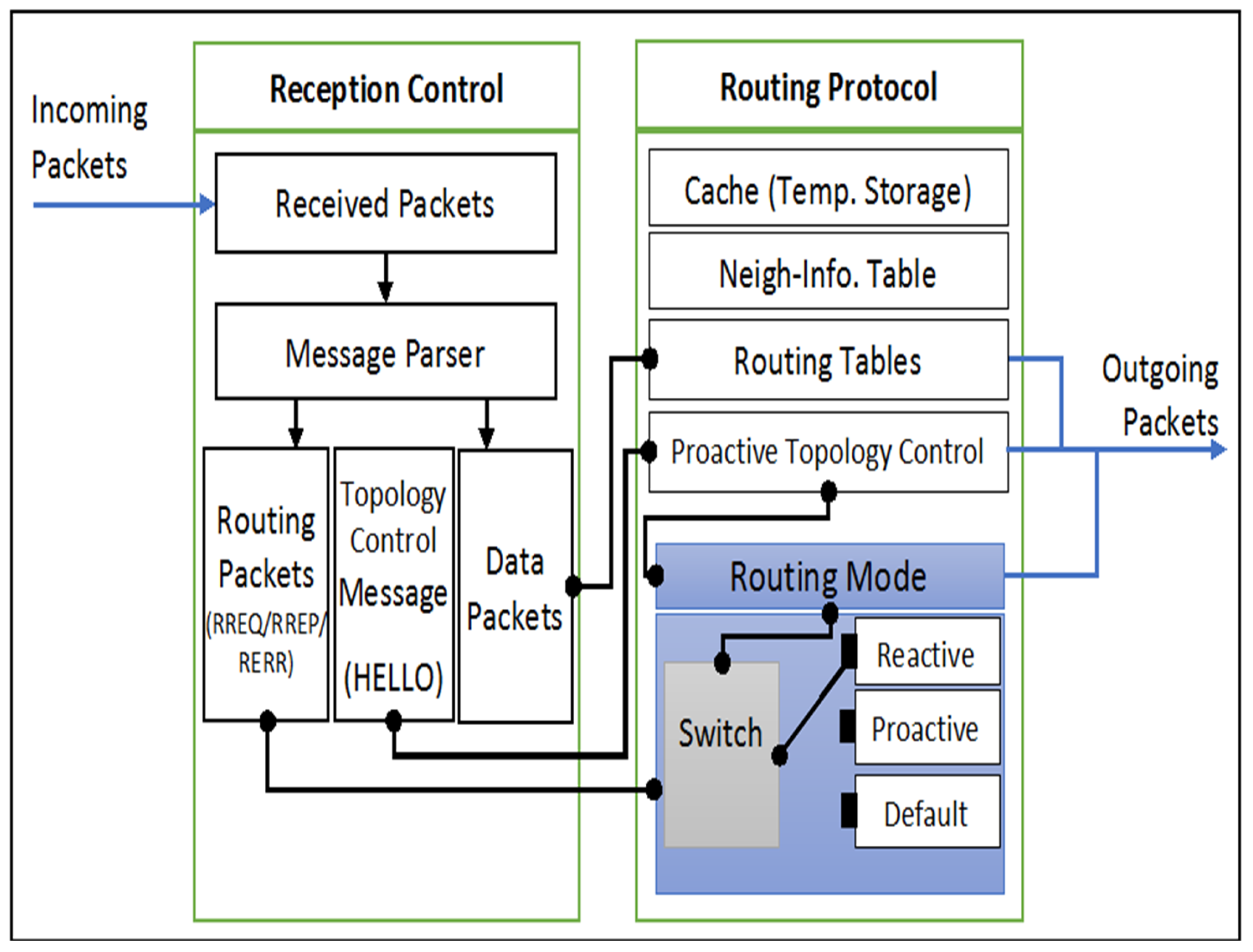
The design of smart nodes, their functions, and the algorithms employed in the mechanism are detailed in this subsection. Various scenarios are presented, along with smart node responses. As previously stated, smart nodes act rationally, allowing different types of communication and data packets to be received and intelligent case-based decisions to be made.

3.4.1. Diagram for Smart Nodes

The architecture of proposed smart nodes is divided into two sections: the first is reception control, which deals with packet recognition and the latter is routing protocol selection. The packet analysis is the subject of the first module. The received packets are classified as (a) data, (b) routing, and (c) TCM packets using a message parser. A different set of instructions is followed for each type of packet. The routing protocol module receives the set of instructions. The routing tables are kept in the routing protocol module. This module additionally adjusts the routing mode based on the previous module’s instructions. This module also keeps track of the neighbors’ information as well as a temporary storage cache. This architecture is presented in Figure 7 and is further explained in Table 7.

Figure 7. Smart node’s architecture.

Table 7. Smart nodes’ operational steps.

S#	Nature of Received Packet	Instructions to Be Followed
1	Received packet (Any type/Protocol)	Verify the message’s type before sending it to the module of routing protocol. Transfer a copy to Cache.
2	Routing Packet (RREQ/RREP/RERR) Protocol: Reactive	Switch to reactive routing mode. Reply/Forward and update/make entries in the Rea-Routing-Table.
3	TC Messages Protocol: Proactive	Send it to TC, switch to Proactive mode, and respond to the sender. In the future, treat the sender as a proactive node. Update the Pro-Routing-Table
4	Data packet Protocol: Any	ACK in case of destination node otherwise forward using the routing table. If there is no appropriate record in the routing tables, do not react. Update/new entry in the routing tables.

3.4.2. Algorithms

This section goes through three major algorithms. Algorithm 1 describes the technique for smart nodes to choose an initial default routing protocol. The selected routing protocol may update with the passage of time, according to the GT process. Algorithm 2 describes how to update the routing protocol. Smart nodes accept packets and conduct different tasks depending on the nature of packets received. Algorithm 3 explains this procedure.

Algorithm 1: Selection of Default Routing Protocol

Input: $n_i$ Output: DefaultRoutingProtocol Begin: $With{ \mathrm{Neigh}}_{\mathrm{Table}}$ $Update \mathrm{Records}$ $Calculate$ $\mathrm{ThE}=\mathrm{Med}\left(\mathsf{\lambda }\mathrm{E}\left({\mathrm{n}}_{\mathrm{j}}\right)\right)$ $\mathrm{ThM}=\mathrm{Med}\left(\mathrm{MobRatio}\right)$ $End With$ $If \mathrm{MobRatio}({\mathrm{n}}_{\mathrm{i}})>\mathrm{ThM}$ $\mathrm{Return} \mathrm{Reactive}$ $Else If \mathsf{\lambda }\mathrm{E}\left({\mathrm{n}}_{\mathrm{i}}\right)>\mathrm{ThE}$ OR $\mathrm{ER}\left({\mathrm{n}}_{\mathrm{i}}\right)>\mathsf{\beta }$ $\mathrm{Return} \mathrm{Proactive}$ $Else \mathrm{Return} \mathrm{Reactive}$ $Else If$

The neighbors’ table is taken first, according to Algorithm 1. By obtaining new information from its known nodes, the smart node updates the entries. The threshold values for energy to consumption ratios and mobility ratios are calculated in stages 4 and 5. The routing mode is determined from step 7 by comparing the node’s data to the estimated threshold values. If the node’s $\mathsf{\lambda }\mathrm{E}$ is larger than or if its remaining energy ratio is greater than $\mathsf{\beta }$ in step 9, the $0<\mathsf{\beta }<100$ represents a coefficient value obtained during simulations.

Algorithm 2: Evolution Process for Default Routing Protocol

Input: $n_i$ Output: DefaultRoutingProtocol Begin: $If \mathrm{CurrentTime} – \mathrm{LastReadTime} > \mathrm{ExpiryInterval}$ $round=0$ $End if$ $if {\mathrm{G}}_{\mathrm{matrix}}=\Delta \mathrm{R}$ $OR {\mathrm{G}}_{\mathrm{matrix}}=\Delta \mathrm{P}$ $if round=0$ $\mathrm{PP}=\mathrm{Count} \mathrm{Distinct}\left(\mathrm{ProRtTable}.\mathrm{NextHop}\right)$ $\mathrm{RP}=\mathrm{Count} \mathrm{Distinct}\left(\mathrm{ReaRtTable}.\mathrm{NextHop}\right)$ $If (\mathrm{PP}>\mathrm{RP})$ $\mathrm{Return} \mathrm{Proactive}$ $Else$ $\mathrm{Return} \mathrm{Reactive}$ $round=1$ $End If$ $Else$ $\mathrm{PP}=\mathrm{Count} \mathrm{Distinct}\left(\mathrm{ProRtTable}.\mathrm{DestIP}\right)$ $\mathrm{PP}=\mathrm{PP}+\mathrm{Count} \mathrm{Distinct}\left(\mathrm{ProRtTable}.\mathrm{NextHop}\right)$ $\mathrm{RP}=\mathrm{Count} \mathrm{Distinct}\left(\mathrm{ReaRtTable}.\mathrm{DestIP}\right)$ $\mathrm{RP}=\mathrm{RP}+\mathrm{Count} \mathrm{Distinct}\left(\mathrm{ReaRtTable}.\mathrm{NextHop}\right)$ If$\left(\mathrm{PP}>\mathrm{RP}\right)$ $\mathrm{Return} \mathrm{Proactive}$ $Else$ $\mathrm{Return} \mathrm{Reactive}$ $round=1$ $End If$ $End If$ $Else$ $\mathrm{Return} {\mathrm{n}}_{\mathrm{i}}.\mathrm{DefltRtProc}$ $\mathrm{LastReadTime}=\mathrm{CurrentTime}$ $End If$

In Algorithm 2, the round variable is utilized to change the evolutionary rounds for parameter consideration. This round gets reset to its original value when a certain amount of time has passed. The time is verified for expiry in step one. If the round has expired, step 2 sets the first round. In step 4, the game matrix is examined for the chances of a degraded routing protocol. If there is a degraded protocol, steps 6 to 12 are carried out for the case of first round, and steps 15 to 23 are carried out for the cases of the next rounds. At first, the node examines the neighbors’ parameters, but in subsequent cases, the node considers all the known nodes in its routing tables.

Algorithm 3: Operational Tasks of Smart Nodes

Input: Packet Output: Begin: $Upon Reception of \mathrm{Packet}$ $Parse \mathrm{Packet}$ $\mathrm{Cache}=\mathrm{Packet}$ $If \mathrm{Packet}.\mathrm{Protocol}=\mathrm{Reactive}$ $\mathrm{R}T=\mathrm{R}eaRtTable$ $Else$ $\mathrm{R}T=ProRtTable$ $End If$ $If \mathrm{Packet}.\mathrm{T}ype=\mathrm{R}outing$ $R{t}_{Pro}.Mode=\mathrm{Reactive}$ $If \mathrm{P}acket.Dest={\mathrm{n}}_{\mathrm{i}}.Address$ $\mathrm{REPLY} Packet.Source$ $Else If Packet.Dest exists in RT.Dest$ $\mathrm{Forward} RT.NextHop$ $Else$ $\mathrm{Broadcast} \mathrm{Packet}$ $Else If$ $\mathrm{Update} ReaRtTable$ $End If$ $If \mathrm{Packet}.\mathrm{T}ype=\mathrm{T}C$ $R{t}_{Pro}.Mode=Pro\mathrm{active}$ $\mathrm{REPLY} Packet.Source$ $\mathrm{Update} ProRtTable$ $End If$ $If \mathrm{Packet}.\mathrm{T}ype=\mathrm{D}ATA$ $if Packet.Dest={\mathrm{n}}_{\mathrm{i}}.Address$ $\mathrm{REPLY} ACK$ $Else If \mathrm{P}acket.Dest \mathrm{e}xists \mathrm{i}n RT.DestIP$ $\mathrm{FORWARD} to RT.NextHop$ $Else$ $\mathrm{REPLY} ERROR$ $End If$ $Enf If$

Algorithm 3 deals with packet arrival and node’s operations regarding the kind of packet. Initially, a temporary variable RT is allocated to one of the routing tables. Step 9 determines whether the packet is of routing type. For a route packet arrival, actions are conducted from steps 10 to 18. The node either acknowledges the source, or broadcasts or forwards the packet during these steps. Step 20 determines whether or not the packet is a proactive TCM. The routing table is modified after the TC message is acknowledged. At step 25, the packet is checked to see if it contains data. Respective operations (steps 26–31) are performed according to the nature of the data packet.

4. Simulation Results

The proposed work is simulated in NS2.35. AWK scripts were used to extract the results from the created trace files, and then MS Excel was used to create the graphs. The performance metrics accessed were remaining energy, throughput, PDR, and end-to-end delays. Some scenarios were created and the results with and without smart nodes were assessed. A heterogeneous network made up of AODV and DSDV nodes was used in these scenarios. The findings are compared with and without the smart nodes. In each example the network is first examined with the absence of nodes that have the proposed mechanism. After that, the proposed mechanism’s smart nodes are added to the network, and outcomes are analyzed. The duration of the simulation was 100 seconds. Table 8 lists the main simulation parameters. In four time pauses, the resultant values were recorded.

Table 8. Common parameters for all the simulations.

Simulation Parameters
Size of Network	1000 m × 1000 m
Type of Channel	WirelessChannel
Ifq Max packets	50
Type of Network interface	WirelessPhy/Phy
Type of MAC	Mac/802_11
Max energy	100 J
Power—Tx	0.9 W
Power—Rx	0.7 W
Power—Idle	0.6 W
Power—Sleep	0.1 W
Type of traffic	CBR
Size of packets	500
Duration of simulation	100 s
Reading times	10, 20, 40, 100

4.1. Case 1: Nodes from Different Classes Are Deployed in Separate but Nearby Fields

Figure 8 shows a screenshot of the NetAnim animator in this scenario. The AODV nodes are green, the DSDV nodes are blue, and the proposed smart nodes are red.

Figure 8. Case scenario 1: NS2 NetAnim Screenshot.

In Table 9, the parameters for heterogeneous nodes are listed. There are three classes of nodes, each with its own set of values. The common and uncommon communication types are considered in this example situation. In the previous section, these types were discussed.

Table 9. Case 1: Parameters for classes of nodes.

Parameters of Nodes
Nodes Type	DSDV	AODV	Smart
Color of nodes	Blue	Green	Red
Number of Nodes	49 (0–48)	49 (49–97)	02 (98,99)
Common-Case Source nodes	0, 1	49, 50	-
Common-Case Destination node	48	97	-
Unusual-Case Source nodes	0, 1	-	-
Unusual-Case Destination Node	-	96, 97	-
Locations	Random with x-axis < 500	Random with 500 < x-axis < 1000	97 at 500, 350 98 at 500, 700

In scenario 1, where there are two classes of nodes coupled together but not overlapped in the area, Figure 9 displays the simulation results for frequent communication instances. Only DSDV nodes can communicate with each other. AODV nodes, on the other hand, only communicate with AODV. Values with and without smart nodes are shown in the graph. When it comes to common communication, smart nodes have a much smaller part in the network. The smart nodes would have formed part of either DSDV or AODV classes of nodes because there is no cross connectivity. If a smart node has the same number of DSDV and AODV neighbors, the reactive protocol will be used until the threshold energy level i.e., β is reached. The results reveal that the performance of such a network is almost unaffected by the presence of smart nodes.

Figure 9. Case 1: Type of common communication.

In the next experiment, the network was assumed to have two source nodes from DSDV class and two destination nodes from AODV destinations nodes for unusual communication. The routing protocols used by the sources and destinations were different. Because such communication is impossible without the smart nodes, the results for “Without Smart Nodes” cannot be calculated because there are no outputs. Only the energies of nodes are reported. Without the usage of smart nodes, the results show that this form of communication is not possible in general. The values for all QoS measures were recorded when the proposed smart nodes were used, as shown in Figure 10. It is worth noting, however, that the amount of remaining energy in the absence of smart nodes is significantly higher. This is because the network nodes cannot establish paths, thus there is no energy spent on routing and data communication.

Figure 10. Case 1: Uncommon communication type.

4.2. Case 2: Heterogeneous Nodes Are Not Placed Distinctly

In the previous section, we discussed this case. In this scenario, we have a network with three classes of nodes: DSDV, AODV, and smart nodes. All these nodes were randomly deployed in the same area. These nodes have positions that overlap in a certain area. The simulation’s NS2 screenshot is shown in Figure 11. The scenario includes 35 DSDV, 35 AODV, and 30 smart nodes.

Figure 11. Case scenario 2: NS2 NetAnim Screenshot.

The simulation parameters for this experiment are given in Table 10.

Table 10. Case 2: Parameters for classes of nodes.

Parameters of Nodes
Type of Nodes	DSDV	AODV	Smart
Color of Nodes	Blue	Green	Red
Number of Nodes	35 (0–34)	35 (35–69)	30 (70–99)
Source nodes	0, 1	35, 36	-
Destination node	34	69	-
Locations	Random	Random	Random

Figure 12 shows the simulation results for Case Scenario 2. Except for energy usage, the network with smart nodes produces significantly better results in all performance parameters. For the smart node-based network, the results for residual energy at various time pauses are virtually identical or slightly better. In the absence of a smart node network, we kept the smart nodes dormant for the simulation. As a result, smart nodes experience minimal energy loss, resulting in superior average remaining energy values.

Figure 12. Case scenario 2: Random placement of heterogeneous nodes.

4.3. Case 3: Proactive Nodes Are Deployed in an L Pattern

In this example, we assume that all of the nodes of a particular class are clustered together in an L shape. The DSDV nodes are considered in this case. A similar instance was described in the previous section. If we do not use the smart nodes, the route entails all of the nodes of DSDV class, which is a lengthier route. The reactive AODV nodes can also be used by incorporating the smart nodes, and a diagonal route can be constructed, minimizing the number of intermediate nodes. Figure 13 depicts the screenshot for case 3. Table 11 shows the parameters used in this case scenario.

Figure 13. Case scenario 3: NS2 NetAnim Screenshot.

Table 11. Case 3: Parameters for classes of nodes.

Parameters of Nodes
Type of Nodes	DSDV	AODV	Smart
Color of Nodes	Blue	Green	Red
Number of Nodes	20 (0–19)	20 (20–39)	20 (40–59)
Source node	9	-	-
Destination node	19	-	-
Locations	Fixed (L Form)	Random	Random

The results for case 3 are shown in Figure 14. With a smart node-based network, the results for PDR, delays, and throughput are better. This is because of the establishment of a shorter route. However, the remaining energy is quite comparable. Because the non-proactive nodes are not employing their energies, less energy is spent without smart nodes. If we simply consider the values of DSDV nodes, the ratio of remaining energy in the absence of smart nodes will be significantly greater. Because the AODV routing burden is taken into account, the throughput of the smart node-based network is high. The AODV nodes were not involved in routing in the absence of smart nodes and so there was minimal routing overhead.

Figure 14. Case scenario 3: Proactive nodes are deployed in an L pattern.

The proposed protocol, identified as GMRP in the simulation results, has been compared with AODV and ZRP for further evaluation. A network of 100 nodes with an area of 1500 ms² was taken. The nodes were programmed with AODV, ZRP and GMRP respectively and results were recorded for 200 pause times. The performance of the protocols in terms of PDR, average energy consumption, and end-to-end latency were accessed. Figure 15, Figure 16 and Figure 17 show the results. We can infer from the results that GMRP is a highly adaptive protocol that reacts to time. The nodes tend to alter their routing behavior as time progresses. This is because the nodes consume their energy with the passage of time. The performance of GMRP is comparable to AODV in terms of energy consumption and PDR. The smart nodes choose to adopt the reactive routing behavior since they initially have greater energies. The performance steadily declines after pause time 100 as a result of the change to proactive routing behavior. In case of end-to-end delays, the protocol performance is similar to AODV in the beginning but improves later. This is also due to the change of routing behavior from reactive to proactive. The nodes gradually start changing their routing protocol with the passage of time by looking into their remaining energies.

Figure 15. Packet delivery ratio (No. of packets received/No. of packets sent).

Figure 16. End-to-end delays (milliseconds).

Figure 17. Average energy consumption (Joules).

5. Conclusions and Future Work

Depending on their capabilities and the nature of their usage, ad hoc networks can take on a variety of configurations. Various ad hoc networks can be linked together for the creation of an efficient and more powerful network. A multimode hybrid routing protocol is proposed in this paper that can be utilized to create a HANET including nodes from diverse ad hoc networks. Moreover, the proposed routing protocol can be implemented in the entire network or a subset of the network nodes. The smart nodes are those nodes that use the proposed routing protocol to communicate. At the same time, the smart nodes preserve the routing tables for both reactive and proactive neighbors. These nodes can adjust their routing behavior adaptively as needed. Furthermore, its default routing protocol is adjusted using a game-theoretic technique. The smart nodes progress through many steps to find the best routing protocol for themselves and the entire network. The energy level and consumption and mobility ratios are the parameters used to establish the default routing protocol for these smart nodes.

We employed AODV and DSDV as base protocols in this work. Instead of these two, any type and number of protocols can be selected. With a set of finite parameters for the network nodes, linear programming can be used to implement numerous protocols by improving normalization and achieving the best solution. The consideration of multiple routing protocols could cause an uncertainty problem. A technique for making decisions under uncertainty can be created by combining game theory and linear programming.