Exploiting Features with Split-and-Share Module

Abstract

Deep convolutional neural networks (CNNs) have shown state-of-the-art performances in various computer vision tasks. Advances on CNN architectures have focused mainly on designing convolutional blocks of the feature extractors, but less on the classifiers that exploit extracted features. In this work, we propose Split-and-Share Module (SSM), a classifier that splits a given feature into parts, which are partially shared by multiple sub-classifiers. Our intuition is that the more the features are shared, the more common they will become, and SSM can encourage such structural characteristics in the split features. SSM can be easily integrated into any architecture without bells and whistles. We have extensively validated the efficacy of SSM on ImageNet-1K classification task, and SSM has shown consistent and significant improvements over baseline architectures. In addition, we analyze the effect of SSM using the Grad-CAM visualization.

1. Introduction

Deep convolutional neural networks (CNNs) achieve high performance in various computer vision tasks [1,2,3,4,5,6,7,8]. A general anatomy of CNN splits the architecture into two parts: a feature extractor and a classifier [9,10,11,12]. A feature extractor consists of conv-blocks which are made of normalization layers, convolutional layers, non-linear activations [13], and pooling layers. To design CNN architecture is to find a good conv-block and stack it repetitively. ResNet [14] added identity-based skip connections to the Conv-block to enable stable training even when the Conv-block is repeatedly stacked deeply. In addition, the Xception [15] structure is a network structure developed from the Inception [16] structure. Xception utilizes Depth-wise-separable convolution using 1x1Conv to significantly lower the computation of the network and even improve its performance. Accordingly, the recent trend on neural architecture search [17,18,19] focuses on designing better conv-blocks in a data-driven way, while the classifier is also a crucial part of a CNN, less attention has been paid on designing better classifiers. In this work, we propose a novel classifier, named Split-and-Share Module (SSM). SSM divides the given feature into several groups of channels, and the groups are partially shared among sub-classifiers. Each group of channels has different degree of sharing and our intuition is that the mostly shared group will contain general features, and vice versa. This feature split-and-share method can encourage the diversity of the features by structure, and thus the diversity of the sub-classifiers, leading to higher performances when ensembled.

Figure 1 shows the structure of the proposed SSM. Given a feature vector extracted from the backbone network (feature extractor), SSM splits the feature into four groups and each group is fed into the designated sub-classifier. The final output is the sum of outputs from each sub-classifier.

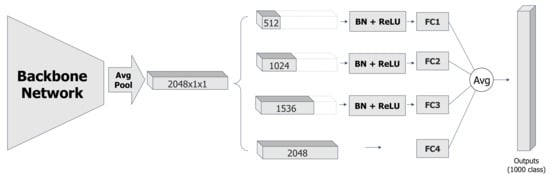
Figure 1. The illustrated example has 2048 channels in the final feature vector, and the output is 1000-class classification (An overview of SSM).

The smallest group, illustrated as the bottom group in Figure 2, is shared by all other sub-classifiers, and should contribute to the final prediction alone. It is encouraged to learn more common and general features in the limited number of channels. On the other hand, the least shared channels, illustrated as the top group in Figure 2, will learn additional features such as contextual information.

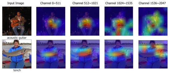
Figure 2. Grad-CAM visualization of channels with respect to sub-classifiers.

The Grad-CAM [20] visualization in Figure 2 qualitatively supports our intuition. As shown in Figure 2, the first column shows the acoustic guitar taken by Grad-CAM for each channel group. We can see that going down from the first row to the bottom row, starting with the additional characteristics of the acoustic guitar and gradually visualizing it as the core characteristic of the acoustic guitar. SSM shows stable performance improvement in architectures such as ResNet [14] and ResNeXt [21], and is a simple structure consisting of BatchNorm [22] and ReLU, easy to attach to any CNN architecture.

While the sub-classifiers may resemble the ensemble technique, which may lead to concerns on less improvements with ensemble. In our experiments, we show that a SSM-augmented network can further be improved with ensemble without any compromises. In this study, we focus on designing a classifier that further exploits a given feature vector. To the best of our knowledge, most of the CNN architectures simply adopt single or multiple linear combinations as the classifier. Our SSM assigns an explicit role to each group by limiting the number of back-propagation between channel groups of the extracted feature. Extensive experiments show that the proposed SSM can induce a significant performance improvement of the model.

2. Related Works

2.1. Deeper Architectures

Starting with AlexNet [23], many CNN structures have been proposed. VGGNet [24] showed significant CNN performance improvement by increasing network depth. Another study made network learning stable by normalizing the input to each layer in batch units. Based on these developments, ResNet was proposed. ResNet proposed identity-based skip connections to deepen the network, greatly improving the performance of CNN. Since then, studies have been proposed to discover CNN structures through architecture search such as NASNet [17] and EfficientNet [19]. Furthermore, architecture search methods based on Evolutionary Algorithms such as AmoebaNet [18] have been proposed. Studies of these CNN structures have been continuously proposed and attracted great attention. However, in the progress of the structure of these CNN classifier has been excluded. We conducted a study using features that were already well extracted from the feature extractor, and can be used in the architecture search later.

2.2. Feature Analysis

Various analyses of features have been proposed [25,26]. Ilyas et al. [27] was experimental in that it exists as robust and non-robust features and can be classified, rather than simply dividing features into useful and useless features. From the perspective of Ilyas et al. [27], there are robust features and non-features among features used for prediction, both of which are useful for prediction but have different meanings and have room to utilize these characteristics.

Afalo et al. [28] showed that using all the features that enter the classifier does not improve the accuracy of the CNN, but removing unnecessary features through pruning can improve the performance and the computational speed of the CNN.

In this respect, our SSM is also a new analysis and utilization of features. Our SSM forcibly assigns the role of features used for prediction through backprop, and qualitatively and quantitatively analyzes the effect on the network according to the location and number of such features.

2.3. Sequential Feature Filtering Classifier

FFC [26] is a study that increases the efficiency of feature maps. The FFC performs channel-wise feature filtering using Layer Normalization and ReLU in Feature-level. Through this process, it can be seen that features of various levels are reproduced and performance is significantly improved in various tasks. In this study, SSM also reprocesses the previously extracted feature map from this point of view and uses it for inference. SSM, which is this study, also reprocesses the previously extracted feature map from this point of view and uses it for inference. The difference from FFC is that SSM forcibly limits the degree of backprop of each feature group, giving the role of each group.

3. Split-and-Share Module

In this section, we describe how SSM is formulated. SSM is a simple classifier that splits and share features with multiple sub-classifiers. The overall architecture of SSM is illustrated in Figure 1, and the pseudo code algorithm is described in Algorithm 1.

First, SSM equally divides the input feature in four splits, and sequentially append the splits one-by-one to formulate four features with different numbers of channels. For example, given the feature $F\in R^{2048}$, the first feature $F_1$ contains the first 1/4 channels, i.e., $F_1=F[0:512]$. Accordingly, $F_2$ contains the first 1/2 channels, and so on. In order to diversify the four features while keeping the feature domain with minimum overheads, we apply BatchNorm with ReLU to the first three features for simple scaling and non-linear activation. The resulting four features will have the same semantic meaning with different scales for the shared channels. Channels in the four features can be zeroed out by ReLU. BatchNorm and ReLU are essential in SSM, as they add extra non-linearity to the overall process. Without BatchNorm and ReLU, SSM can be reduced to a simple linear combination (fully-connected) layer. After splitting, recombining and re-scaling, the four features are feed-forwarded to four sub-classifiers. Each sub-classifier is a simple fully-connected layer, where the output dimension is the number of classes. The final output of SSM is the average of the four outputs from the sub-classifiers.

The key intuition of our design is to partially share the given feature. The first 1/4 channels are shared among all sub-classifiers. These channels are forwarded four times and back-propagated four times. As they are most frequently used channels, we expect these channels are trained to be the most important key features. In contrast, the last 1/4 channels are used only by the last sub-classifier, so they are expected to contain some additional features, such as context information on the surrounding environments. We visualized the four splits of channels with the Grad-CAM visualization technique in Figure 2 and Figure 3, and more analysis will be discussed in Section 5.

Algorithm 1 Split-and-Share Module

1: procedure SSM($features,num\_channels$=2048, $num\_heads$=4) 2:      $n\leftarrow$INT$(num\_channels$ / $num\_heads$) 3:      $v\leftarrow \left[\right(empty\_list)$] 4:      for i=1 to $num\_heads$ do 5:           $out\leftarrow features[:i\ast n]$ 6:           $out\leftarrow$BatchNorm$\left(out\right)$ 7:           $out\leftarrow$ReLU$\left(out\right)$ 8:           $out\leftarrow$FC$\left(out\right)$ 9:           v.append($out$) 10:     end for 11:     $result\leftarrow v$.sum() / $num\_heads$ 12:     return $result$ 13: end procedure

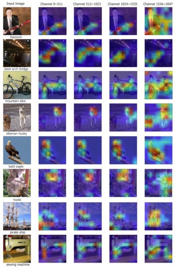
Figure 3. Additional Grad-CAM visualization results.

4. Experiments

In this section, we validate the efficacy of the proposed SSM on various architectures, and analyze the effect of SSM in several aspects. First, we use SSM upon ResNet and ResNeXt architectures in ImageNet-1K classification dataset [1]. SSM has shown performance improvements in most cases, and details will be described in Section 4.1. In Section 4.2, we describe the ablation studies of SSM.

4.1. ImageNet-1K Classification

The ImageNet-1K dataset [1] consists of 1.28 million training images and 50 k validation datasets. During training, the images are resized to 256 × 256 shape, and randomly cropped to 224 × 224 patches with random horizontal flipping. During testing, the images are also resized to 256 × 256 shape, and a single 224 × 224 patch is cropped at the center. For both training and testing, images are normalized with the mean and standard deviation of all pixels in the dataset. We adopt He’s method [29] for network random initialization. We use SGD optimizer with base learning rate 0.1 and batch size of 256. The running rate is reduced by one-tenth at epoch 30 and 60, and the total number of epochs is 90. The weight decay value is set to 0.0001 and the momentum value is set to 0.9.

The experiment result is summarized in Table 1. SSM has consistently improved performance in all the architectures, except ResNet-18 that does not improve. The distinctive difference between ResNet-18 and other architectures is that the final feature of ResNet-18 has 512 channels, while others have 2048 channels. Therefore, we assume that the number of channels in the final feature should be large enough for SSM to be effective.

Table 1. Classification results on ImageNet-1K. Single-crop validation errors are reported.

Architecture	Dataset	Epoch	Top-1 Acc
ResNet-18 [14]	ImageNet-1K	90	70.04%
ResNet-18 [14] + SSM	ImageNet-1K	90	70.05% (+0.01%)
ResNet-50 [14]	ImageNet-1K	90	75.65%
ResNet-50 [14] + SSM	ImageNet-1K	90	76.68% (+1.03%)
ResNet-101 [14]	ImageNet-1K	90	76.62%
ResNet-101 [14] + SSM	ImageNet-1K	90	77.93% (+1.31%)
ResNeXt50 [21]	ImageNet-1K	90	77.19%
ResNeXt50 [21] + SSM	ImageNet-1K	90	77.96% (+0.77%)
ResNeXt101 [21]	ImageNet-1K	90	78.46%
ResNeXt101 [21] + SSM	ImageNet-1K	90	79.68% (+1.22%)

In all architectures except ResNet-18, the performance improvement is significant. Furthermore, the absolute improvements in larger architectures are greater than the smaller ones. ResNet-101 improves 1.31% in the top-1 accuracy, while ResNet-50 improves 1.03%; ResNeXt-101 improves 1.22%, while ResNeXt-50 improves 0.77%.

4.2. Ablation Studies and Analysis

4.2.1. Training Scheme for Sub-Classifiers

There are two simple ways to train the four sub-classifiers: apply the classification loss to individual sub-classifier outputs, or apply the loss to the average of the outputs. The former one requires each sub-classifier to independently learn to classify, and then ensemble the four sub-classifiers; the latter one allows the sub-classifiers to jointly learn to classify. The results are summarized in Table 2. SSM is the result of training with the loss given to the averaged output, SSM-individual is the result of training each output independently. When individually trained, the sub-classifiers’ performances are much higher than the jointly trained ones. Interestingly, the final ensemble performance is significantly higher in the jointly trained one. The result indicates that jointly training the sub-classifiers will encourage the sub-classifiers to have different roles to create synergy, and thus the final ensemble performance is higher than the independently trained one.

Table 2. Results of ImageNet-1K classification according to two different training schemes.

Architecture	Dataset	FC1 Acc	FC2 Acc	FC3 Acc	FC4 Acc	Averaging Acc
ResNet-50 [14] + SSM	ImageNet-1K	65.24%	73.24%	75.09%	1.02%	76.68%
ResNet-50 [14] + SSM-individual	ImageNet-1K	75.60%	75.11%	76.18%	74.77%	75.38%

4.2.2. Is SSM a New Way of Ensemble?

Ensemble is a simple technique to further boost performance by combining multiple models that have different random initializations. The sub-classifiers of SSM may resemble the ensemble technique, and there may be concerns that SSM benefits from the ensemble-like effect and thus may not benefit from ensemble. However, we argue that SSM is not simply an ensemble method, and we validate that SSM-augmented models can further benefit from ensemble.

We train two ResNet-50 models and two ResNet-50 + SSM models with different initializations, and test if SSM can further benefit from ensembles. The results are summarized in Table 3. In the same environment, We separately train the two models for two times each. The two ResNet-50 + SSM models accuracies are 76.37% and 76.68%, and the ensembled accuracy is 78.04%, which is 1.35% higher. The improvement is a little less than the ResNet-50 ensemble, but it may be simply due to the performance saturation, and the 1.35% is still a significant improvement by ensemble. Therefore, through this experiment we show that SSM-augmented models can further benefit from ensemble.

Table 3. Results of ensemble classification in ImageNet-1K.

Architecture	Dataset	Epoch	Top-1 Accs	Ensembled Acc
ResNet-50 [14]	ImageNet-1K	90	75.60%, 75.65%	77.25% (+1.60%)
ResNet-50 [14] + SSM	ImageNet-1K	90	76.37%, 76.68%	78.04% (+1.35%)

4.2.3. Is the Improvement Simply Due to Parameter Increases?

Finally, we show that the efficacy of SSM is not simply due to parameter increase. To verify this, we further train two models with more parameters by adding more parallel classifiers. As shown in Table 4, the base ResNet-50 has 25.55 M parameters, and ResNet-50 + SSM has 28.58 M parameter, so the parameter overhead is 3.03 M. One fully connected layer has 2.05 M parameters, so we add one or two parallel fully connected layers to the baseline ResNet-50. ResNet-50 (2FC) and ResNet-50 (3FC) are the new comparison methods that brings additional parameters in the classifier part, like SSM. The result is summarized in Table 4. A simple increase in parameters, like ResNet-50 (2FC) and (3FC), does not improves the performance much, but SSM does bring a significant improvement. Therefore, we argue that the performance improvement is not simply due to parameter increase, but due to the feature exploiting characteristics of SSM.

Table 4. The result of the parameter increase in ImageNet-1K. In all experiments, FC was added vertically, and all were ensembled using the averaging method.

Architecture	Dataset	Epoch	Top-1 Acc	Parameters
ResNet-50 [14]	ImageNet-1K	90	75.65%	25.55 M
ResNet-50 [14] (2FC)	ImageNet-1K	90	75.91%	27.60 M
ResNet-50 [14] (3FC)	ImageNet-1K	90	75.67%	29.65 M
ResNet-50 [14] + SSM	ImageNet-1K	90	76.68%	28.63 M

5. Qualitative Analysis

The key intuition of SSM is to partially share the features among different sub-classifiers. As described in Section 3, the first 1/4 channels are shared among all sub-classifiers, and the last 1/4 channels are used only by the last sub-classifier. The first 1/4 channels are the most frequently feed-forwarded and back-propagated, and are expected to contributes mostly to the final prediction of SSM. In short, our hypothesis is that the degree of sharing is positively correlated with the importance of the feature. Therefore, the first 1/4 channels are expected to contain the key features to classify among the target classes, and the last 1/4 channels are expected to contain additional features such as contextual information.

We qualitatively analyze the channels with the Grad-CAM visualization. Figure 2 and Figure 3 shows input images from the validation set and the overlaid Grad-CAM heatmaps with respect to the ground-truth labels. ResNet-50+SSM is the visualization target. To analyze whether the feature splits have learned differently, the visualizations are generated for each 1/4 split of channels, instead of the full feature. The column ‘Channel 0~511’ denotes the Grad-CAM of the first 1/4 channels with respect to the first sub-classifier. The column ‘Channel 512~1023’ denotes the visualization of the second 1/4 channels w.r.t. the second sub-classifier, and so on, while the input to the second sub-classifier is the first 1/2 channels, we visualized the second 1/4 to explicitly compare the semantics learned in each 1/4 channels.

The samples in Figure 2 and Figure 3 supports our intuition. The Grad-CAMs for the first sample in Figure 2 demonstrate that the first 1/4 channels focus on the ground-truth ‘guitar’ location, and the last 1/4 channels focus on the corresponding context, which in this case is the guitar player. The two intermediate Grad-CAMs gradually changes from the key feature of the guitar to the corresponding context of the guitar player. The Grad-CAMs of the second sample in Figure 2 also show that the first 1/4 channels focus on the fish, and the last 1/4 channels focus on the corresponding context of the river. We demonstrate more samples in Figure 3. In summary, the Grad-CAM visualizations for each split channels show that the most shared channels focus on the target object, and the least shared channels focus on the corresponding context information.

6. Discussion

We experimented with how much performance improvement would be achieved by selecting the best inferred output of each output and using it for prediction in the ResNet-50+SSM structure learned from the training set of ImageNet-1K. We have not yet developed an algorithm to select the optimal FC, so we have selected the optimal FC by ourselves, utilizing the label data of ImageNet-1K. The result was that if FC could be ideally chosen, an additional 6% performance improvement could be seen with up to 82.9% performance. Further research on this part is believed to be possible. By developing the methodology of SSM, it can be actively used in fields that actively utilize the characteristics of features, such as semantic segmentation or action recognition.

7. Conclusions

We propose Split-and-Share Module (SSM). SSM is a classifier that improves the performance of CNN networks. We apply the BatchNorm and ReLU to the shared features extracted from the feature extractor, limiting the number of commonly used and non-featured backprops, and have an effect of learning by placing weights on important features. Through this process, features learned according to importance have a classifier suitable for their capacity, and averaging multiple outputs from the classifier for use in training and testing. We verified SSM by applying CNNs of various structures in ImageNet-1K, and showed significant performance improvement in all the experiments. We also adopted Grad-CAM for qualitative analysis of SSM. Grad-CAM results showed qualitatively that our SSM could learn according to the importance of features as we intended. In addition, SSM divides the features into four groups and learns common and non-specific features, which are considered to be available in many research fields that actively utilize the features map with these characteristics of SSM’s unique characteristics.

References

- Deng, J.; Dong, W.; Socher, R.; Li, L.J.; Li, K.; Fei-Fei, L. Imagenet: A large-scale hierarchical image database. In Proceedings of the 2009 IEEE Conference on Computer Vision and Pattern Recognition, Miami, FL, USA, 20–25 June 2009; pp. 248–255. [Google Scholar]
- Lin, T.Y.; Maire, M.; Belongie, S.; Hays, J.; Perona, P.; Ramanan, D.; Dollár, P.; Zitnick, C.L. Microsoft coco: Common objects in context. In European Conference on Computer Vision; Springer: Berlin/Heidelberg, Germany, 2014; pp. 740–755. [Google Scholar]
- Cordts, M.; Omran, M.; Ramos, S.; Rehfeld, T.; Enzweiler, M.; Benenson, R.; Franke, U.; Roth, S.; Schiele, B. The cityscapes dataset for semantic urban scene understanding. In Proceedings of the IEEE Conference on Computer Vision and Pattern Recognition, Las Vegas, NV, USA, 27–30 June 2016; pp. 3213–3223. [Google Scholar]
- Kuehne, H.; Jhuang, H.; Garrote, E.; Poggio, T.; Serre, T. HMDB: A large video database for human motion recognition. In Proceedings of the 2011 International Conference on Computer Vision, Barcelona, Spain, 6–13 November 2011; pp. 2556–2563. [Google Scholar]
- Bocu, R.; Bocu, D.; Iavich, M. Objects Detection Using Sensors Data Fusion in Autonomous Driving Scenarios. Electronics 2021, 10, 2903. [Google Scholar] [CrossRef]
- Hwang, D.Y.; Choi, S.H.; Shin, J.; Kim, M.; Choi, Y.H. GAN-Based ROI Image Translation Method for Predicting Image after Hair Transplant Surgery. Electronics 2021, 10, 3066. [Google Scholar] [CrossRef]
- Ciborowski, T.; Reginis, S.; Weber, D.; Kurowski, A.; Kostek, B. Classifying Emotions in Film Music—A Deep Learning Approach. Electronics 2021, 10, 2955. [Google Scholar] [CrossRef]
- Peng, Z.; Gong, X.; Wei, B.; Xu, X.; Meng, S. Automatic Unsupervised Fabric Defect Detection Based on Self-Feature Comparison. Electronics 2021, 10, 2652. [Google Scholar] [CrossRef]
- Bengio, Y.; Courville, A.; Vincent, P. Representation learning: A review and new perspectives. IEEE Trans. Pattern Anal. Mach. Intell. 2013, 35, 1798–1828. [Google Scholar] [CrossRef]
- Sengan, S.; Kotecha, K.; Vairavasundaram, I.; Velayutham, P.; Varadarajan, V.; Ravi, L.; Vairavasundaram, S. Real-Time Automatic Investigation of Indian Roadway Animals by 3D Reconstruction Detection Using Deep Learning for R-3D-YOLOV3 Image Classification and Filtering. Electronics 2021, 10, 3079. [Google Scholar] [CrossRef]
- Mai, D.T.; Ishibashi, K. Small-Scale Depthwise Separable Convolutional Neural Networks for Bacteria Classification. Electronics 2021, 10, 3005. [Google Scholar] [CrossRef]
- Alsharif, R.; Al-Issa, Y.; Alqudah, A.M.; Qasmieh, I.A.; Mustafa, W.A.; Alquran, H. PneumoniaNet: Automated Detection and Classification of Pediatric Pneumonia Using Chest X-ray Images and CNN Approach. Electronics 2021, 10, 2949. [Google Scholar] [CrossRef]
- Nair, V.; Hinton, G.E. Rectified linear units improve restricted boltzmann machines. In Proceedings of the 27th International Conference on Machine Learning (ICML-10), Haifa, Israel, 21–24 June 2010; pp. 807–814. [Google Scholar]
- He, K.; Zhang, X.; Ren, S.; Sun, J. Deep residual learning for image recognition. In Proceedings of the IEEE Conference on Computer Vision and Pattern Recognition, Las Vegas, NV, USA, 27–30 June 2016; pp. 770–778. [Google Scholar]
- Chollet, F. Xception: Deep learning with depthwise separable convolutions. In Proceedings of the IEEE Conference on Computer Vision and Pattern Recognition, Honolulu, HI, USA, 21–26 July 2017; pp. 1251–1258. [Google Scholar]
- Szegedy, C.; Liu, W.; Jia, Y.; Sermanet, P.; Reed, S.; Anguelov, D.; Erhan, D.; Vanhoucke, V.; Rabinovich, A. Going deeper with convolutions. In Proceedings of the IEEE Conference on Computer Vision and Pattern Recognition, Boston, MA, USA, 7–12 June 2015; pp. 1–9. [Google Scholar]
- Zoph, B.; Vasudevan, V.; Shlens, J.; Le, Q.V. Learning transferable architectures for scalable image recognition. In Proceedings of the IEEE Conference on Computer Vision and Pattern Recognition, Salt Lake City, UT, USA, 18–23 June 2018; pp. 8697–8710. [Google Scholar]
- Real, E.; Aggarwal, A.; Huang, Y.; Le, Q.V. Regularized evolution for image classifier architecture search. In Proceedings of the AAAI Conference on Artificial Intelligence, Honolulu, HI, USA, 27 January–1 February 2019; Volume 33, pp. 4780–4789. [Google Scholar]
- Tan, M.; Le, Q.V. Efficientnet: Rethinking model scaling for convolutional neural networks. arXiv 2019, arXiv:1905.11946. [Google Scholar]
- Selvaraju, R.R.; Cogswell, M.; Das, A.; Vedantam, R.; Parikh, D.; Batra, D. Grad-cam: Visual explanations from deep networks via gradient-based localization. In Proceedings of the IEEE International Conference on Computer Vision, Venice, Italy, 22–29 October 2017; pp. 618–626. [Google Scholar]
- Xie, S.; Girshick, R.; Dollár, P.; Tu, Z.; He, K. Aggregated residual transformations for deep neural networks. In Proceedings of the IEEE Conference on Computer Vision and Pattern Recognition, Honolulu, HI, USA, 21–26 July 2017; pp. 1492–1500. [Google Scholar]
- Ioffe, S.; Szegedy, C. Batch normalization: Accelerating deep network training by reducing internal covariate shift. arXiv 2015, arXiv:1502.03167. [Google Scholar]
- Krizhevsky, A.; Sutskever, I.; Hinton, G.E. Imagenet classification with deep convolutional neural networks. Adv. Neural Inf. Process. Syst. 2012, 25, 1097–1105. [Google Scholar] [CrossRef]
- Simonyan, K.; Zisserman, A. Very deep convolutional networks for large-scale image recognition. arXiv 2014, arXiv:1409.1556. [Google Scholar]
- Lee, S.W.; Lee, R.; Seo, M.S.; Park, J.C.; Noh, H.C.; Ju, J.G.; Jang, R.Y.; Lee, G.W.; Choi, M.S.; Choi, D.G. Multi-Task Learning with Task-Specific Feature Filtering in Low-Data Condition. Electronics 2021, 10, 2691. [Google Scholar] [CrossRef]
- Seo, M.; Lee, J.; Park, J.; Kim, D.; Choi, D.G. Sequential Feature Filtering Classifier. IEEE Access 2021, 9, 97068–97078. [Google Scholar] [CrossRef]
- Ilyas, A.; Santurkar, S.; Tsipras, D.; Engstrom, L.; Tran, B.; Madry, A. Adversarial examples are not bugs, they are features. arXiv 2019, arXiv:1905.02175. [Google Scholar]
- Aflalo, Y.; Noy, A.; Lin, M.; Friedman, I.; Zelnik, L. Knapsack Pruning with Inner Distillation. arXiv 2020, arXiv:2002.08258. [Google Scholar]
- He, K.; Zhang, X.; Ren, S.; Sun, J. Delving deep into rectifiers: Surpassing human-level performance on imagenet classification. In Proceedings of the IEEE International Conference on Computer Vision, Santiago, Chile, 7–13 December 2015; pp. 1026–1034. [Google Scholar]
Publisher’s Note: MDPI stays neutral with regard to jurisdictional claims in published maps and institutional affiliations. |
© 2022 by the authors. Licensee MDPI, Basel, Switzerland. This article is an open access article distributed under the terms and conditions of the Creative Commons Attribution (CC BY) license (https://creativecommons.org/licenses/by/4.0/).