Multilevel Pyramid Network for Monocular Depth Estimation Based on Feature Refinement and Adaptive Fusion

Abstract

As a traditional computer vision task, monocular depth estimation plays an essential role in novel view 3D reconstruction and augmented reality. Convolutional neural network (CNN)-based models have achieved good performance for this task. However, in the depth map recovered by some existing deep learning-based methods, local details are still lost. To generate convincing depth maps with rich local details, this study proposes an efficient multilevel pyramid network for monocular depth estimation based on feature refinement and adaptive fusion. Specifically, a multilevel spatial feature generation scheme is developed to extract rich features from the spatial branch. Then, a feature refinement module that combines and enhances these multilevel contextual and spatial information is designed to derive detailed information. In addition, we design an adaptive fusion block for improving the capability of fully connected features. The performance evaluation results on public RGBD datasets indicate that the proposed approach can recover reasonable depth outputs with better details and outperform several depth recovery algorithms from a qualitative and quantitative perspective.

1. Introduction

Recovering scene depth information from monocular images/videos has always been an essential issue in the field of 3D vision. The purpose is to measure the distance from each pixel in the scene to the camera. In recent years, monocular depth estimation (MDE) has attracted substantial attention because it occupies an essential role in 3D scene understanding and many vision applications, such as robotics [1], augmented reality [2], and stereo conversion [3]. However, as an ill-posed issue, MDE requires additional information such as shadows, color changes, layout, and texture information in the image to help us predict pixel-level depth information. This additional prior knowledge can disambiguate different 3D scales through learning-based methods. However, such methods are not suitable for all scenarios due to the impracticality of requiring prior knowledge. Currently, compared with traditional learning-based methods in MDE, several approaches utilizing convolutional neural networks (CNNs) [4,5,6,7,8,9,10] have shown overwhelming advantages. However, due to a series of downsampling operations performed during feature extraction at the encoding part, the estimated depth maps lack local details, especially for distant objects. Many researchers have observed this issue and have explored solutions for enhancing depth details. Some researchers use dilated convolutions [11,12] to increase the receptive field. Another way is to connect low-level features at the encoder part with high-level features at the decoder part through skip connections [13]. In addition, some scholars try to solve this problem by extracting multiscale context features [14,15,16]. These end-to-end frameworks can achieve reasonable results, but there are some limitations. For example, in feature extraction processes at the encoder part, some methods ignore the spatial features of RGB images while only considering extraction of contextual features. Some methods directly connect features via skip connections. However, low-level features at the encoder part need further enhancement and refinement, as they cannot reflect details of object edges and small structures well.

Recently, the attention mechanism has been widely utilized for feature enhancement and refinement in MDE [17,18,19,20]. Inspired by this, we design an efficient multilevel attention pyramid network for MDE on the basis of feature refinement and adaptive fusion. Unlike most depth estimation algorithms that only acquire contextual features, this study also considers the extraction of spatial features. Specifically, we design a spatial feature extraction scheme that feeds a series of downsampled versions of color images into a spatial feature extraction block to obtain multi-scale information with better edge details. In addition, a spatial attention-based feature refinement module that combines and enhances this multilevel information is designed to derive detailed information. Recent studies have shown that full connection and fusion of multilevel features can greatly recover local details. Therefore, fully connected fusion is used to enrich the representation of each level feature. Since the contributions of different levels of fully connected features are different, we also design an adaptive fusion block to fuse different levels of features.

The contributions of the present network are:

• In addition to extracting contextual features, we also developed a multilevel spatial feature generation module to extract rich spatial features containing better details.
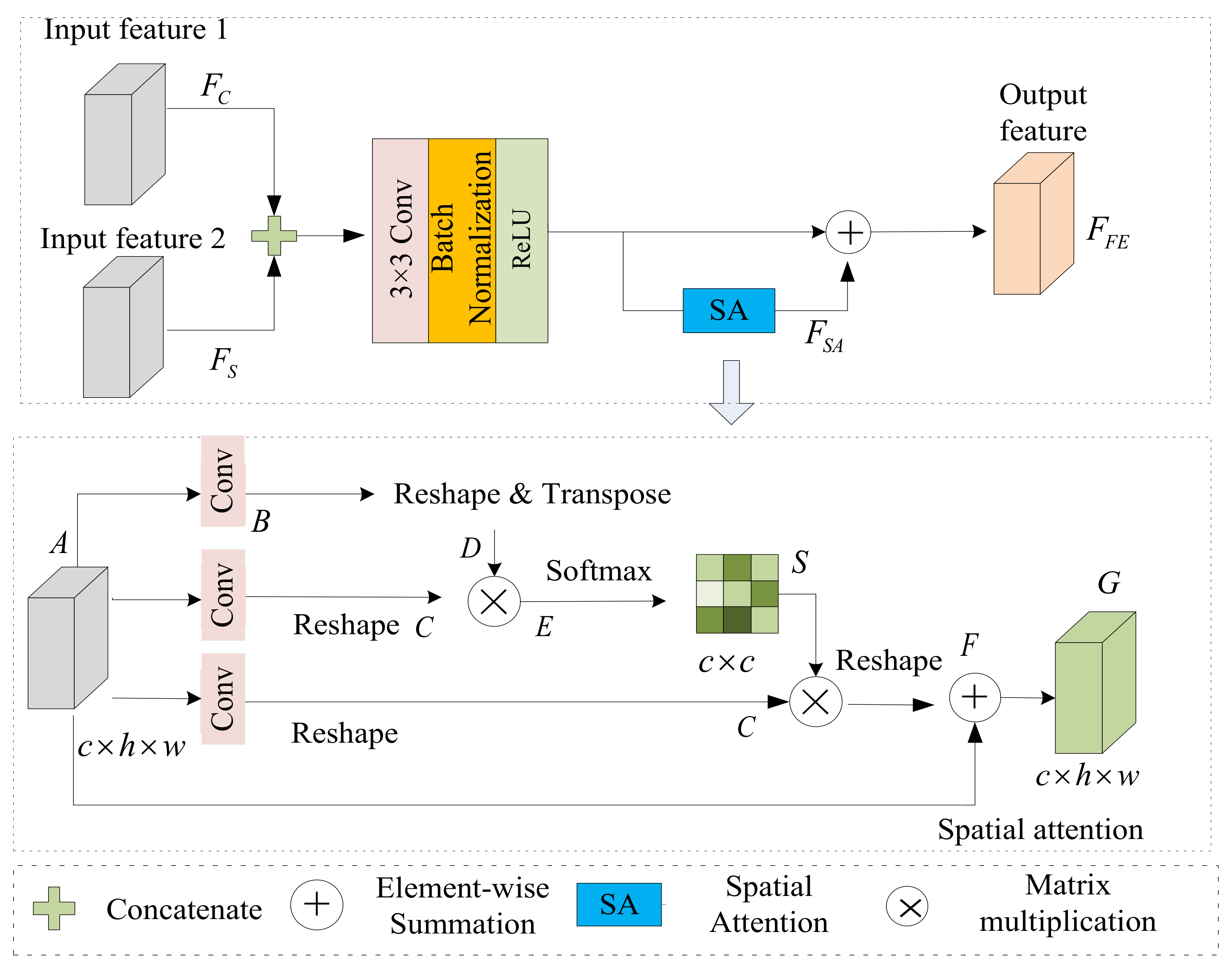
• We designed a spatial attention-based feature refinement module that enhances multilevel information to derive detailed information.
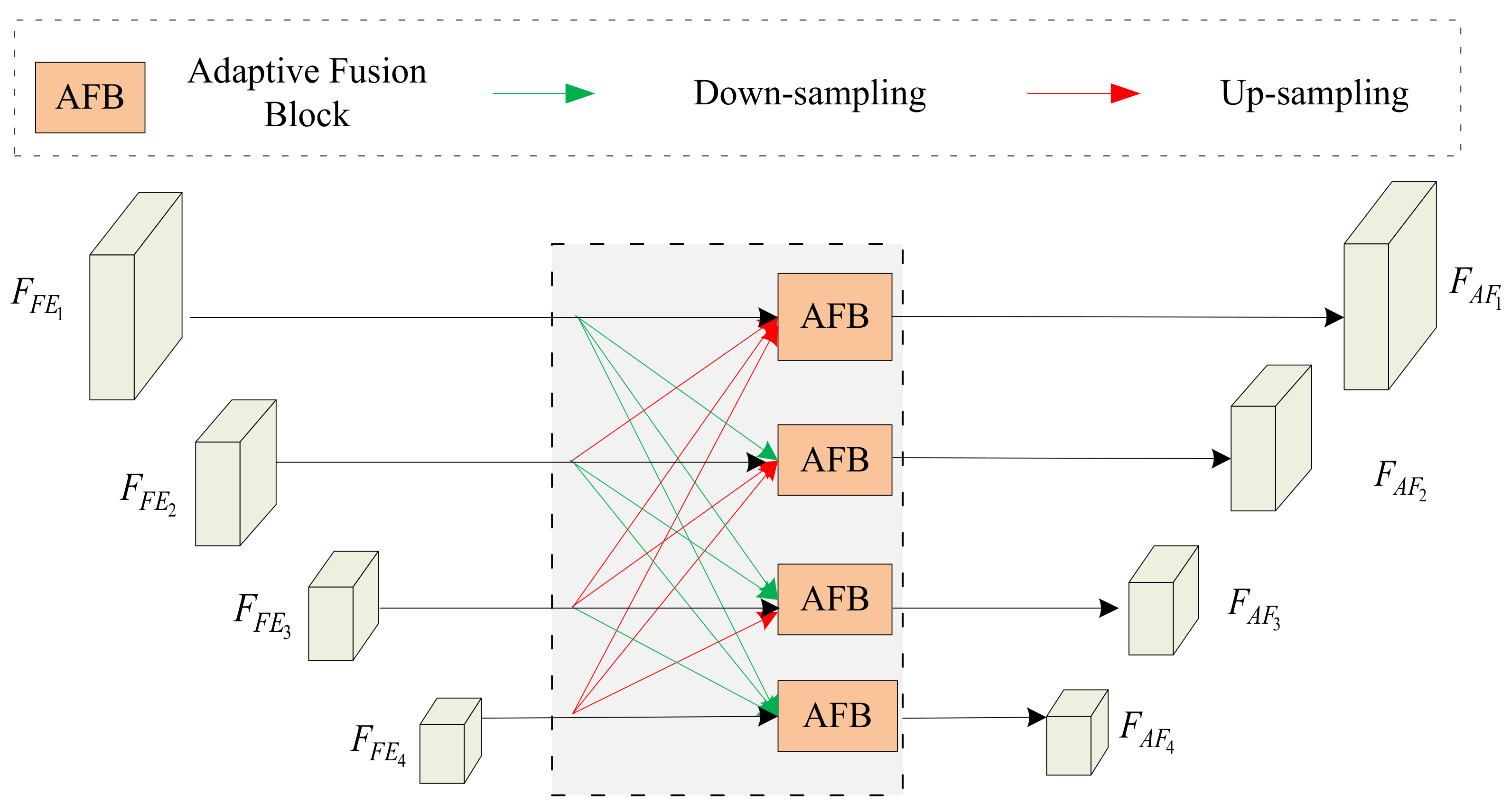
• We utilized fully connected fusion to enrich the representation of each level feature. Moreover, an adaptive fusion block is designed to fuse fully connected features according to the reliability of features.
• An efficient hybrid loss function and loss terms reweighted scheme are explored for multilevel outputs to provide depth details.

The rest of this study is organized as follows. The related works are described in Section 2. Section 3 introduces our framework. Section 4 analyses the experimental results. Finally, conclusions and future research are presented in Section 5.

2. Related Work

2.1. Supervised Learning

We categorize current MDE methods into supervised and self-supervised learning methods according to whether ground truth depths are leveraged during training. For supervised learning-based depth recovery methods, the purpose is to determine the mapping relationship between color images and depth maps by training on an RGB-D dataset. In recent years, with the promotion of convolutional neural networks (CNNs) in vision tasks, an increasing number of researchers have devoted themselves to the development of depth prediction models premised on deep learning. Initiating this line of research, Eigen et al. [4] presented a coarse-to-fine network architecture based on a CNN to obtain reasonable depth maps. To improve the performance of predicted depths, some methods integrate conditional random field (CRF) models into deep structures. For instance, Liu et al. [21] developed an efficient depth prediction model that combines deep CNNs and continuous conditional random fields (CRFs) and obtained reasonable results. Moreover, some methods leverage auxiliary information to refine the details of depth outputs. In parallel, some researchers have devoted themselves to multiscale information extraction for enhancing the ability of feature representations and obtaining depths with more details. Authors in Ref. [22] proposed a deep ordinal regression network (DORN) based on atrous convolution and designed an efficient depth encoder for attaining depth maps with high resolution. To address the problem of spatial information loss, Ye et al. [17] presented a detail-preserving depth recovery network that can preserve spatial and contextual depth details. They designed a nonlocal attention module and combined it with multiscale atrous convolution. Pei et al. [18] presented a multiscale feature network (MSFNet) for MDE. They designed an enhanced diverse attention module and an upsampling stage fusion module that can provide more detailed information. Chen et al. [19] presented an efficient context aggregation network (ACAN), which can learn pixel-level attention maps for long-range contextual information. Song et al. [23] developed an efficient method that decomposes decoding process by exploiting a Laplacian pyramid. To generate clearer depth maps and integrate spatial cues robustly, Wu et al. [24] introduced a side-predictive aggregation method to efficiently embed scene structure information from low-level to high-level. To improve depth prediction accuracy, they also introduced a continuous spatial refinement loss at multiple resolutions. Since information exchange between different tasks has great advantages, many researchers have begun to explore multitask learning. For instance, Gao et al. [25] designed an efficient framework to jointly learn depth prediction and semantic labeling tasks. In their study, they developed a feature-sharing module to integrate discriminative features from different tasks. Zhao et al. [26] presented a multitask scheme that contains contour recovery, salient detection, and depth reconstruction tasks to detect salient objects. They developed a multimodal filtered transformer block for enhancing features from each modality. Moreover, there are also several other methods. To solve the problem of algorithm generalization, Wang et al. [27] proposed a CNNapsule network for monocular depth estimation. They extracted CNN and Matrix Capsule features and designed a fusion block to fuse the two. The authors design a loss function that combines long-tailed distributions, gradients, and structural similarity. For the problem of sacrificing computational complexity and efficiency for high accuracy, Liu et al. [28] proposed a fast encoder-decoder network (EdgeNet) for edge devices. They also designed a low-complexity upsampling module to aggregate global depth information. On the basis of ensuring accuracy, they also developed a channel pruning method to further reduce computational complexity.

2.2. Self-Supervised Learning

Since ground truth depth labels are not required in their training processes, self-supervised learning methods have become a popular topic in the MDE field. In 2019, Godard et al. [29] designed a versatile model for self-supervised monocular depth recovery. To solve the occlusion and dynamic object issues in self-supervised learning, they designed a minimum reprojection loss and an automatic mask loss, respectively. Reasonable outputs can be generated by this method. However, ambiguous reprojection still exists in this method. To address this problem, Watson et al. [30] introduced depth hints method, which improves an existing photometric loss term. Wong et al. [31] presented residual-based adaptive weight and bilateral loop consistency constraints to enhance the performance of depth recovery in the edge region to handle the problems of large pixel changes and discontinuous gradients in the edge region. The authors in Ref. [32] proposed a multiscale feature extractor to extract monocular image features and fine-tune the errors of the prediction results using proxy labels. Ling et al. [33] developed an efficient framework for unsupervised depth reconstruction on the basis of attention mechanism. They also designed an efficient multi-distribution reconstruction loss, which enhances the capability of the network by amplifying the error during view synthesis. Ye et al. [34] designed a dual-network framework that contains a monocular branch and a stereo branch. The monocular network predicts the coarse depths of monocular images. Taking coarse depths and stereo image pairs as input, the stereo network further mines the stereo information. Sun et al. [35] jointly estimated depth and visual odometry in the framework of unsupervised learning and designed a depth pose consistency loss term to study geometric constraints between different training samples. In parallel, a new dynamic receptive field network based on residual networks was designed by Chiu et al. [36], which can assign suitable receptive fields for images with different resolutions to estimate high-quality depths. Recently, transformers have also started to be generally utilized in self-supervised MDE. Varma et al. [37] developed a self-supervised depth prediction approach from monocular images on the basis of transformers and compared the performance of transformer and CNN-based methods on KITTI dataset. Yang et al. [38] proposed a simplified transformer for self-supervised depth estimation. The designed simplification strategy, joint attention mechanism, and connection mechanism can reduce model complexity. This model can be directly generalized to other dense image prediction tasks such as semantic segmentation. Some methods utilize information about the target model itself to improve its performance. For instance, Mendoza et al. [39] used a self-distillation method to build a self-supervised monocular depth estimation model. To strengthen the consistency between predictions, they studied consistency enforcement strategy and employ auxiliary strategies to filter out unreliable predictions.

3. Proposed Method

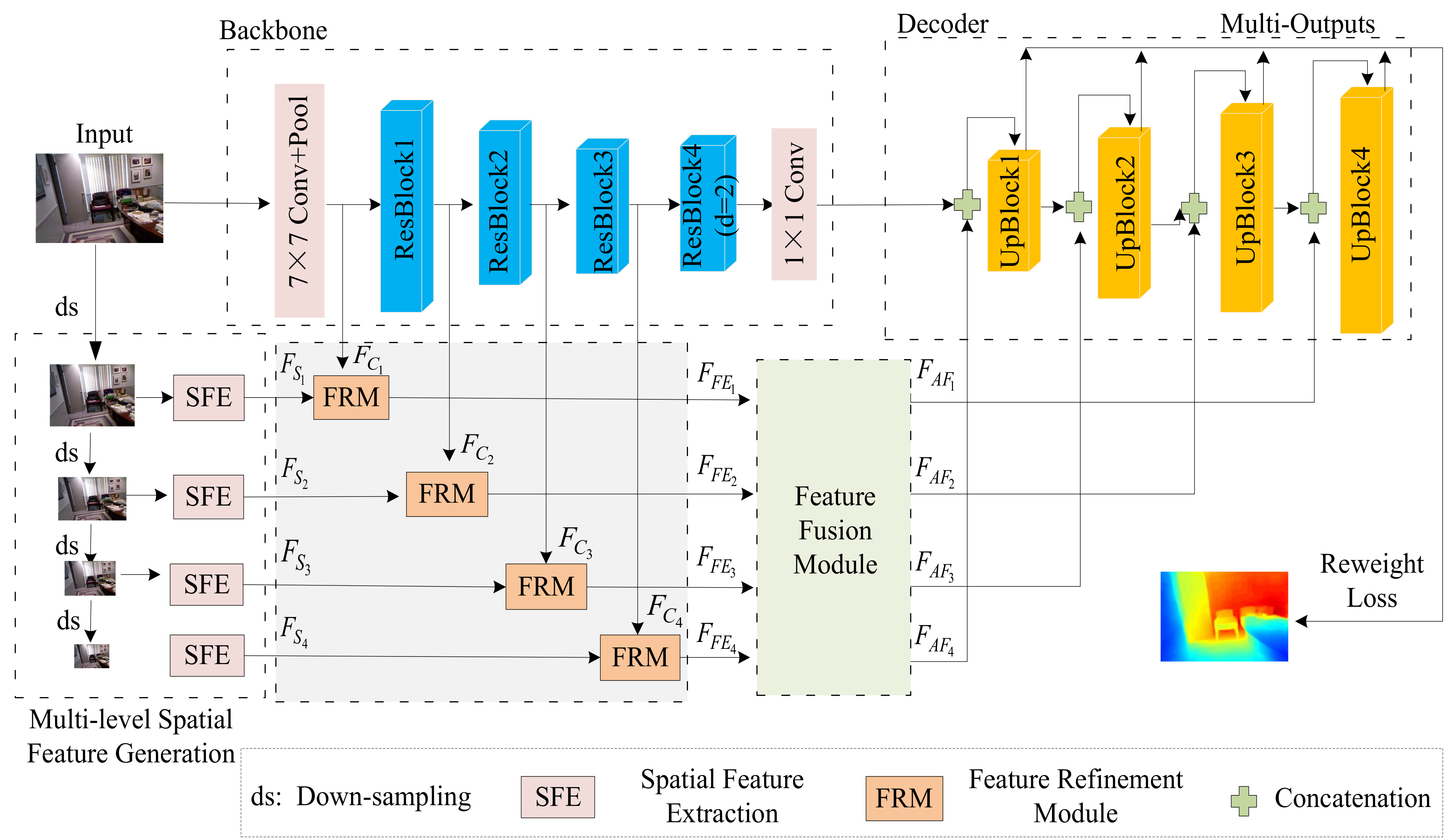
3.1. Network Architecture

To predict precise depth outputs with better details, we present an efficient multilevel pyramid network for MDE on the basis of feature refinement and adaptive fusion. Figure 1 presents the overall architecture of the framework. The network includes five parts: a backbone network, a multilevel spatial feature generation module (MSFGM), a feature refinement module (FRM), a feature fusion module (FFM), and a decoder. In the first part, a multilevel feature extraction module is designed for receiving multilevel depth feature maps. It contains a contextual branch and a spatial branch. In the contextual branch, ResNet-101 is utilized as our backbone network. We then send the feature map output from the backbone network into a convolution block to generate the contextual features of the encoder part. In the spatial branch, the downsampled color images are sent into a spatial feature extraction module to generate a set of features with different resolutions. The features of each level from two branches are fed into a feature refinement module. In addition, a feature refinement module is developed on the basis of spatial attention to combine and enhance multilevel information to derive detailed information. Recent studies have shown that full connection and fusion of multilevel features can greatly combine local details. Therefore, we apply fully connected fusion to enrich the representation of each level feature. Since the contributions of different levels of fully connected features are different, we also develop an adaptive fusion block to fuse different levels of features. Then, the adaptively fused multilevel features are fed into the decoder part, which can increase the resolution of low-resolution depth maps. We fed these outputs into consecutive upsampling blocks to generate multilevel outputs and integrate these multilevel outputs via the loss reweighting method to generate the final depths.

Figure 1. The overall architecture of our framework. It contains five parts: backbone network, multilevel spatial feature generation module (MSFGM), feature refinement module (FRM), feature fusion module (FFM), and decoder. We use ResNet-101 as our backbone. MSFGM is designed for receiving abundant spatial feature maps. FRM can effectively integrate and enhance contextual and spatial features, whereas FFM adaptively fuses fully connected multiscale features. Then, multilevel features obtained from FFM are fed into the decoder to recover precise outputs with high resolution.

3.2. Multi-Level Spatial Feature Generation Module (MSFGM)

To address the problem of local depth detail loss, a multilevel framework is designed to generate more meaningful spatial and contextual information. Our present scheme generates multiscale features $F_{C_i}=\left\{F_{C_1},F_{C_2},F_{C_3},F_{C_4}\right\}$ from the contextual branch network and obtains multiscale features $F_{S_i}=\left\{F_{S_1},F_{S_2},F_{S_3},F_{S_4}\right\}$ from the spatial branch network for an input color image. For the contextual branch, the original ResNet-101 is used as our backbone network. Different from the original network, we replace downsampling operators in ResBlock4 with dilated convolution (the dilation rate is set to 2) to maintain the resolution of the depth at a larger size. Then, we feed the feature outputs obtained from the backbone network into convolution layer. The final features $F_{C_i}$ can be generated from the backbone network for a single color image $I$. Features $F_{S_i}$ can be obtained from the spatial branch network for an input color image $I$. The spatial branch collects features from the downsampled color images by utilizing the spatial feature extraction scheme. We first send the downsampled color images into a spatial feature block to generate spatial outputs. The flow chart of spatial feature extraction is shown in Figure 2. We generate the final $F_S$ by combining downsampling process and spatial feature extraction process as follows:

$${\theta }_i=d{s}^{\downarrow i}\left(I\right),$$

(1)

$${\mu }_i=Hf\left({\theta }_i\right),$$

(2)

$$f_{CBR1i}=Relu\left(BatchNorm\left(Con{v}_{3\times 3}\left({\mu }_i\right)\right)\right),$$

(3)

$$f_{CBR2i}=Relu\left(BatchNorm\left(Con{v}_{3\times 3}\left(f_{CBR1i}\right)\right)\right),$$

(4)

$$F_{S_i}=Con{v}_{3\times 3}\left(f_{CBR2i}\right),$$

(5)

where $d{s}^{\downarrow i},i=1,2,3,4$ represents the downsampling operation. The resolution of the original image is decreased to $1/2$, $1/4$, $1/8$, and $1/16$ through downsampling. $Con{v}_{3\times 3}$ denotes a convolution with a $3\times 3$ kernel. Here, $Hf$ denotes a filtering operation, where an ideal high-pass filter with a cutoff frequency radius of 80 is used; $BatchNorm$ and $Relu$ refer to the processes of batch normalization and ReLU, respectively; and $Con{v}_{3\times 3}$ indicates a convolution operation with $3\times 3$ kernels. $f_{CBR{1}_i}$ and $f_{CBR{2}_i}$ denote the output features from two CBR layers.

Figure 2. Spatial feature extraction block.

3.3. Feature Refinement Module (FRM)

The attention mechanism has been leveraged in many visual tasks and has proven to enhance the performance of depth prediction tasks. Motivated by these efforts, we design an attention-based feature refinement module that uses a spatial attention block to extract meaningful features. Figure 3 shows a flowchart of feature refinement module. For a color input image, two types of features can be obtained through a multilevel feature generation module. We intensify features $F_C$ and $F_S$ globally to obtain more effective information via the feature refinement process. Figure 2 shows a flowchart of the feature refinement module. Input features 1 and 2 represent features $F_C$ and $F_S$ obtained from the contextual branch network and spatial branch network, respectively. We concatenate these input features and then send them into a CBR network layer ($3\times 3$ convolution, batch normalization, and ReLU) to reduce feature dimensions. Finally, the connected feature and attention feature obtained from the spatial attention (SA) [40] block are summed to obtain the final global feature. These procedures are described as follows:

$$f=Relu\left(BatchNorm\left(Con{v}_{1\times 1}\left(Concat\left(F_S,F_C\right)\right)\right)\right),$$

(6)

$$F_{FE}=f\oplus F_{SA}\left(f\right),$$

(7)

where $F_{FE}$ is the final feature map; $f$ is the feature map operated by concatenation, convolution, batch normalization, and ReLU; $Con{v}_{1\times 1}$ indicates a convolution operation with $1\times 1$ kernels; $\oplus$ represents the element-wise summation; $concat$ is concatenation operation, and $F_{SA}$ represents attention feature map obtained by spatial attention block. To improve the expressive capability of local features, spatial attention is introduced to encode richer contextual and spatial information into local features. We obtain three identical feature maps $B$ by feeding input features $A\left(c\times h\times w\right)$ into a $1\times 1$ convolution layer. Then, two of these feature maps are reshaped to $C\left(hw\times c\right)$, and another feature map is reshaped and transposed to $D\left(c\times hw\right)$. Next, we apply matrix multiply $C$ and $D$ and feed the result $E$ into a softmax layer to generate the features $S\left(c\times c\right)$. Then, operation of matrix multiplication between $S$ and $C$ is performed. Finally, the multiplied feature map is reshaped and summed with the input feature $A$ to generate the enhanced feature. The feature refinement process is as follows:

$$\begin{array}{l}{F}_{FE}=A\oplus F\\ =A\oplus Reshape\left(S\otimes C\right)\\ =A\oplus Reshape\left(softmax\left(C\otimes D\right)\otimes C\right)\\ =A\oplus Reshape\left(\begin{array}{l}softmax\left(\left(Reshape \left(Con{v}_{1\times 1}\left(X\right)\right)\right){\left(Reshape\left(Con{v}_{1\times 1}\left(X\right)\right)\right)}^T\right)\\ \otimes \left(Reshape\left(Con{v}_{1\times 1}\left(X\right)\right)\right)\end{array}\right)\end{array},$$

(8)

where $Conv{ }_{1\times 1}$ indicates $1\times 1$ convolution layer; $Reshape$ and $Softmax$ are reshape operation and softmax operations, respectively.

Figure 3. Feature refinement module.

3.4. Feature Fusion Module (FFM)

Here, we design a fully connected scheme and an adaptive fusion scheme to fuse these enhanced deep features. We obtain meaningful information from deep features at other levels to enrich the feature representation at the current level via the fully connected scheme. Since the contributions of different levels of fully connected features are different, we also develop an adaptive fusion block to fuse different levels of features efficiently. The feature fusion process is shown in Figure 4. Specifically, four feature representations with the same resolution are generated by a series of upsampling or downsampling interpolations for each level feature. These four feature maps can be described as follows:

$${\widehat{F}}_{Inpu{t}_1}=\left\{F_{F{E}_1}, u{p}^{\uparrow 2}\left(F_{F{E}_2}\right), u{p}^{\uparrow 4}\left(F_{F{E}_3}\right), u{p}^{\uparrow 8}\left(F_{F{E}_4}\right)\right\},$$

(9)

$${\widehat{F}}_{Inpu{t}_2}=\left\{d{s}^{\downarrow 2}\left(F_{F{E}_1}\right), F_{F{E}_2}, u{p}^{\uparrow 2}\left(F_{F{E}_3}\right), u{p}^{\uparrow 4}\left(F_{F{E}_4}\right)\right\},$$

(10)

$${\widehat{F}}_{Inpu{t}_3}=\left\{d{s}^{\downarrow 4}\left(F_{F{E}_1}\right), d{s}^{\downarrow 2}\left(F_{F{E}_2}\right), F_{F{E}_3}, u{p}^{\uparrow 2}\left(F_{F{E}_4}\right)\right\},$$

(11)

$${\widehat{F}}_{Inpu{t}_3}=\left\{d{s}^{\downarrow 8}\left(F_{F{E}_1}\right), d{s}^{\downarrow 4}\left(F_{F{E}_2}\right), d{s}^{\downarrow 2}\left(F_{F{E}_3}\right),F_{F{E}_4}\right\},$$

(12)

where ${\widehat{F}}_{inpu{t}_i}$ denotes the concatenated features at the $i_{th}$ level; $u{p}^{\downarrow }$ represents upsampling operation; $d{s}^{\downarrow }$ represents downsampling operation; and $concat$ is the concatenation operation.

Figure 4. Feature fusion module.

The multilevel feature representations mentioned above are passed to the adaptive fusion block for obtaining a more reasonable combination. We take the multilevel features of the second level as input to illustrate the adaptive fusion process. The adaptive fusion process at the second level is shown in Figure 5. In AFB, these four feature maps are first concatenated as follows:

$${\widehat{F}}_{F{E}_2}=concat\left(d{s}^{\downarrow 2}\left(F_{E{F}_1}\right), F_{E{F}_2}, u{p}^{\uparrow 2}\left(F_{E{F}_3}\right), u{p}^{\uparrow 4}\left(F_{E{F}_4}\right)\right)=concat\left(F_{F{E}_{21}},F_{F{E}_{22}},F_{F{E}_{23}},F_{F{E}_{24}}\right),$$

(13)

Figure 5. Adaptive fusion block.

Then, we perform an average pooling operation for compressing the concatenated features and compute channel statistics. The compressed features pass through a convolution block (CB), which includes a $3\times 3$ convolution, a ReLU activation operation and a $3\times 3$ convolution. Next, we apply sigmoid function to generate the fusion coefficients for features at different levels. Finally, we aggregate weighted multilevel features to generate the final output of the second level. The calculation process is as follows:

$$W_2=S\left(Con{v}_{3\times 3}\left(ReLU\left(Con{v}_{3\times 3}\left(AP\left({\widehat{F}}_{F{E}_2}\right)\right)\right)\right)\right),$$

(14)

$$F_{A{F}_2}={\displaystyle \sum _{j=1}^4{W}_{2j}\cdot }{F}_{A{F}_{2j}},$$

(15)

where $F_{A{F}_2}$ denotes the combined feature and $W_{2j}$ denotes four fusion coefficients for different features at the second level. Since the fusion coefficient depends on the interdependence between features at the same level, the adaptively fused features are more reasonable than direct concatenation or elementwise summation.

3.5. Loss Function

Another key to improving the depth prediction method is the design of the loss function to be used during training. At present, there are some commonly used loss functions, such as ${\ell }_1$, ${\ell }_2$, and the BerHu loss, but they are very sensitive to errors that occur at the edge of the step. To overcome this problem and predict a more reasonable depth output with better local details, a hybrid loss function that contains the BerHu loss, gradient loss, and relative loss is designed. We adopt the BerHu loss as the first loss term, as it combines advantages of the regularly utilized ${\ell }_1$ loss and ${\ell }_2$ loss. The BerHu loss is as shown in Equation (16):

$$L_{berhu}\left(d,d^{*}\right)=\frac{1}{N}{\displaystyle \sum _{p=1}^N{\rm B}\left(e_p\right),}{\rm B}\left(e_p\right)=\left\{\begin{array}{cc}\left|e_p\right|& \left|e_p\right|\le \mathrm{c}\\ \frac{e_p^2+c^2}{2c}& \left|e_p\right|>\mathrm{c}\end{array}\right.,e_p=\left|d-d_p^{\ast }\right|,$$

(16)

where $e_p$ indicates absolute error; we set threshold $c$ as 1/5 of the maximum per-batch error for all pixels. The recovered depths and ground truth depths can be represented by $d$ and $d_{}^{\ast }$, respectively. The second loss term $L_{\mathrm{gra}}$ is utilized to penalize the edge structure changes in both $x$ and $y$ directions, which can be determined as follows:

$$L_{gra}\left(d,d_{}^{*}\right)=\frac{1}{N}{\displaystyle \sum _{p=1}^N\left(\ln \left(\left({\Delta }_x\left(\left|d_p-d_p^{*}\right|\right)\right)+{\alpha }_1\right)+\ln \left(\left({\Delta }_y\left(\left|d_p-d_p^{*}\right|\right)\right)+{\alpha }_2\right)\right)},$$

(17)

where ${\Delta }_x$ and ${\Delta }_y$ indicate the gradient of difference with respect to $x$ and $y$, respectively. Inspired by the feature similarity defined by Zhang et al. [41], a new FSIM loss term $L_{FSIM}$ was designed in this study to measure the feature similarity between two depth maps. The upper bound of FSIM metric is 1; thus, FSIM loss is indicated as below:

$$L_{FSIM}\left(d,d_{}^{*}\right)=\frac{1}{N}{\displaystyle \sum _{p=1}^N\frac{1-FSIM\left(d_p,d_p^{*}\right)}{2}},$$

(18)

The relative loss is used to define the ordinal relationship of sampled pairs between two depth maps. On the basis of the work in Ref. [42], we propose a new relative loss that assigns weights according to the correctness of ordinal relationship. The loss term can be described as follows:

$$L_{\mathrm{rel}}={\displaystyle \sum _{p=1}^N{L}_{r,p}}=\left\{\begin{array}{cc}{\displaystyle \sum _{p=1}^N{w}_p^{\gamma }\log \left(1+\exp \left(-r_p\left(d_p-d_p^{\ast }\right)\right)\right)}& r_p\ne 0\\ {\displaystyle \sum _{p=1}^N{\left(d_p-d_p^{\ast }\right)}^2}& r_p=0\end{array}\right.,$$

(19)

$$w_p^{}=1-1/\left(1+\exp \left(-r_p\left(d_p-d_p^{\ast }\right)\right)\right),$$

(20)

where $r_p$ denotes the ground–truth ordinal relationship. For a particular pixel, this value is set to −1 if the predicted depth value is less than the ground truth depth value, 0 if the predicted depth value is equal to the ground truth depth value, and 1 otherwise. $w_p$ is the weight assigned to sample pairs. We perform a weighted summation of these three loss terms to obtain loss function $L$ as follows:

$$L\left(d,d^{*}\right)={\lambda }_b{L}_{berhu}\left(d,d^{*}\right)+{\lambda }_g{L}_{gra}\left(d,d^{*}\right)+{\lambda }_r{L}_{rel}\left(d,d^{*}\right),$$

(21)

where ${\lambda }_b,{\lambda }_g,{\lambda }_r$ are weights of the Berhu loss, gradient loss, and relative loss, respectively. As mentioned in Section 3.1, we can generate multilevel depth outputs $d=\left\{d_1,d_2,\dots ,d_n\right\}$ with different resolutions from the decoder part. These estimated depth maps are then evaluated according to the loss function. Unlike several previous algorithms that directly give weights, our model focuses more on depth maps with larger sizes and assigns more weight to depth maps with larger resolutions. The final loss function can be calculated as Equation (22):

$$\widehat{L}=\frac{1}{n}{\displaystyle \sum _{i=1}^n\frac{1}{2^i}}{L}_i\left(d_i-d_i^{*}\right),$$

(22)

where $n$ is the number of multistage outputs; $L_i$ is the depth loss of the $i_{th}$ level. $d_i$ and $d_i^{\ast }$ indicate the predicted depth and the ground truth depth of the $i_{th}$ level.

4. Experimental Results

Implementation and training details: We carried out the experiments on a PC platform with an i7-10710, 1.10 GHz CPU, 16 GB RAM, and an RTX2080 GPU. The PyTorch framework was used for model training, and the parameters of ResNet-101 layers trained on the ImageNet dataset were utilized for model initialization. In our study, the momentum of the Adam optimizer was set as 0.99. The base learning rate is initially set to 0.0003, and the learning rate decay is set to 0.1. The weight decay has a value of 0.00004.

Datasets and Metrics: The proposed method was evaluated for outdoor and indoor scenarios. Specifically, we used two RGBD datasets for evaluation: the NYU Kinect V2 dataset [43] and the KITTI dataset [44]. We calculated errors and accuracies from the perspective of the following four evaluation metrics:

(1)

Root-mean-squared error (RMSE(lin)): $\sqrt{\frac{1}{S}{\displaystyle \sum _{p=1}^S{\left(d_p-d_p^{\ast }\right)}^2}}$;

(2)

Root-mean-squared error (RMSE(log)): $\sqrt{\frac{1}{S}{\displaystyle \sum _{p=1}^S{\left(log\left(d_p\right)-log\left(d_p^{\ast }\right)\right)}^2}}$;

(3)

Mean log10 error (log10): $\frac{1}{S}{\displaystyle \sum _{p=1}^S{‖{\log }_{10}{d}_p-{\log }_{10}{d}_p^{\ast }‖}_1}$;

(4)

Mean relative error (Rel): $\frac{1}{S}{\displaystyle \sum _{p=1}^S\frac{{‖d_p-d_p^{\ast }‖}_1}{d^{\ast }}}$;

(5)

Threshold ($th$): percentage of $d_p$, i.e., $\max \left(\frac{d_p^{\ast }}{d_p},\frac{d_p}{d_p^{\ast }{}_P}\right)=\delta <th$.

where $d_p$ denotes the recovered depths and $d_p^{\ast }$ is the ground-truth depths of pixel $p$; $S$ indicates the number of pixels in measured depth maps.

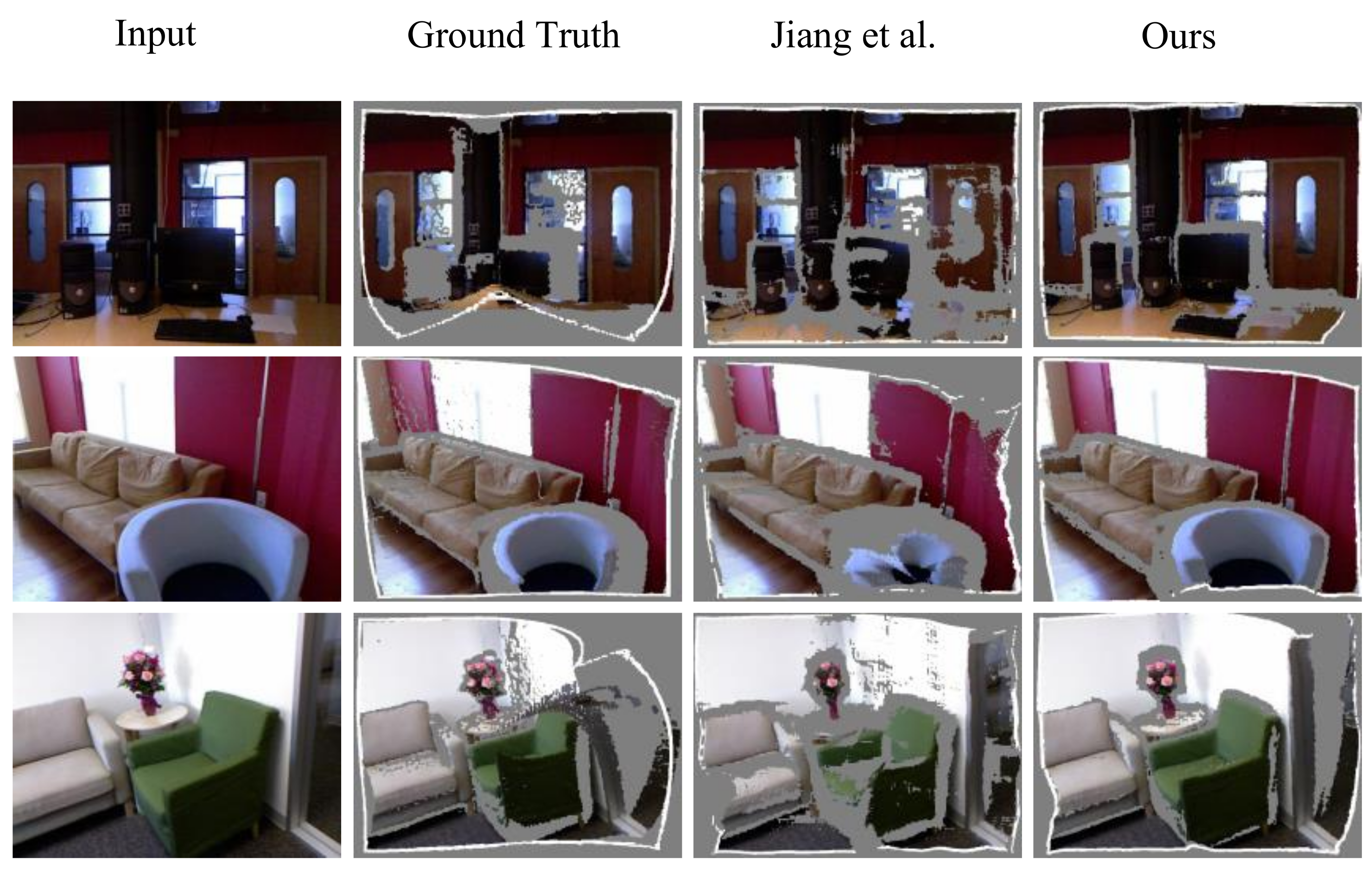
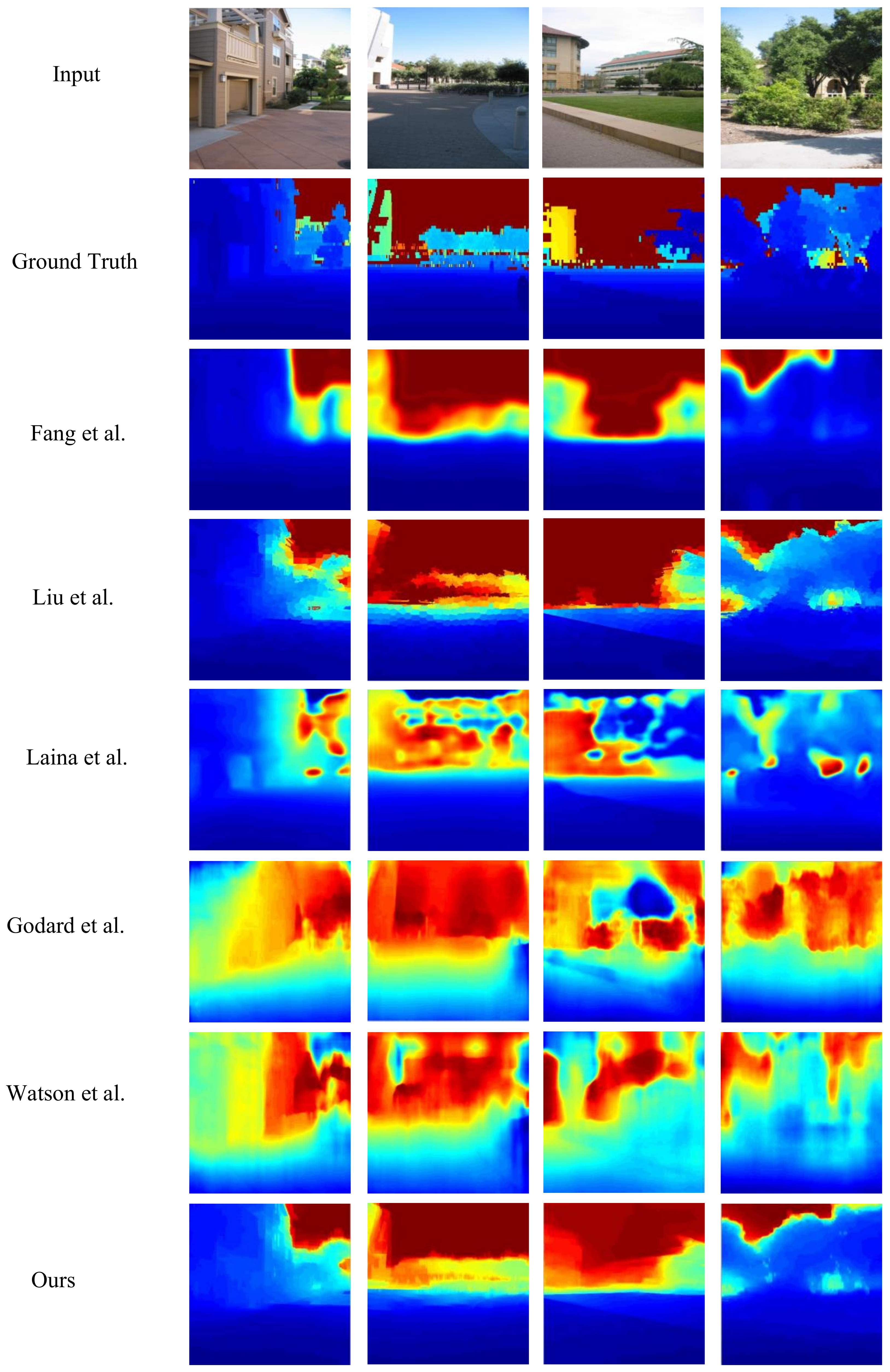
4.1. Qualitative Comparison

The results of the experiments on the NYUv2 dataset are reported in Table 1, in which our method is compared with other depth recovery approaches [4,5,17,18,21,22,45,46,47,48,49,50,51,52]. By analyzing Table 1, Lee et al. [50] explored relative depth and achieved optimal values for metrics and δ < 1.253. By utilizing attention mechanisms and multi-scale convolutions with adaptive weight adjustment for predicting depths, Liu et al. [52] obtained the best log10 and Rel scores. Thanks to our designed spatial feature extraction scheme, feature refinement module, adaptive fusion module, effective loss function, and loss terms reweighting scheme, the presented framework obtained the lowest RMSE(lin), Rel, and δ < 1.25² values and achieved better log10 and δ < 1.25³ values of 0.049 and 0.993, respectively. Our method improved the performance by approximately 0.001 compared to the second-place method under RMSE(lin) criterion. Here, RMSE(lin) represents the deviation between the estimated values and the ground truth values and is often utilized to measure the prediction results of machine learning models. A lower RMSE(lin) value indicates that the presented method has reasonable validity. Additionally, Pei et al. [18] designed an enhanced diverse attention module and upsampling stage fusion module which can provide more detailed information whereas Fu et al. [22] designed an efficient depth encoder for attaining depth maps with high resolution. Both methods perform well.

Table 1. Quantitative comparison results on NYU dataset.

Methods	RMSE(lin)	log10	Rel	δ < 1.25	δ < 1.252	δ < 1.253
Eigen et al. [4]	0.907	NR	0.215	0.611	0.887	0.971
Carvalho et al. [45]	0.600	0.059	0.135	0.819	0.957	0.987
Moukari et al. [46]	0.569	0.057	0.133	0.830	0.966	0.993
Xu et al. [47]	0.586	0.052	0.121	0.811	0.954	0.987
Liu et al. [21]	0.824	0.095	0.230	0.614	0.883	0.971
Laina et al. [5]	0.573	0.055	0.127	0.811	0.953	0.988
Jiang et al. [48]	0.468	0.054	0.127	0.841	0.966	0.993
Wang et al. [49]	0.497	NR	0.128	0.845	0.966	0.990
Lee et al. [50]	0.538	NR	NR	0.837	0.971	0.994
Fu et al. [22]	0.509	0.051	0.115	0.828	0.965	0.992
Ye et al. [17]	0.474	0.063	NR	0.784	0.948	0.986
Pei et al. [18]	0.531	0.051	0.118	0.865	0.975	0.993
SharpNet [51]	0.502	NR	0.139	0.836	0.966	0.990
Liu et al. [52]	0.523	0.049	0.113	0.872	0.975	0.993
Our method	0.463	0.049	0.115	0.868	0.977	0.993

The assessment results for the KITTI dataset from a qualitative perspective are displayed in Table 2. In the table, “Stereo” denotes self-supervised learning by using stereo supervision, whereas “Depth” indicates the supervised learning-based methods by using depth supervision. We compared our method with other competing methods [5,17,18,29,30,31,32,33,34,53,54,55,56,57]. Notably, Liu et al. [53] employed dense depth data, whereas our network used ground truth sparse data for training. By directly using the sparse depth information obtained by lidar, the image preprocessing steps can be omitted. Due to the multilevel spatial feature extraction scheme, feature refinement strategy, and feature fusion scheme, our method obtained the lowest values on the Rel metric and achieved 0.895, 0.974, and 0.990 for δ < 1.25, δ < 1.25² and δ < 1.25³ metrics, respectively. From data in the table, Chen et al. [56] generated the best RMSE(lin) score and has the best performance for RMSE(log). Although RMSE(lin) and RMSE(log) values of our method were not the best, they also reached 3.842 and 0.185, respectively. Table 3 represents the quantitative evaluation outputs of our approach and other methods [5,17,21,29,33,47,52,58,59,60] on the Make3D dataset. Liu et al. [21] developed an efficient depth prediction model that combines deep CNNs and continuous conditional random fields (CRFs), whereas Laina et al. [5] designed fully convolutional residual networks. Kim et al. [59] designed a deep prediction network and a deep gradient recovery network and effectively fused depth information and gradient information. On the whole, the methods of Liu et al. [21] and Laina et al. [5] obtained reasonable results but presented unsatisfactory performance for RMSE(lin), log10, and Rel metrics. Kim et al. [59] obtained the lowest Rel score, whereas our method achieved the best performance for RMSE(lin) and log10. In addition, we achieved significantly better performance on the Rel index.

Table 2. Quantitative comparison results on KITTI dataset.

Methods	Type	RMSE(lin)	Rel	RMSE(log)	δ < 1.25	δ < 1.252	δ < 1.253
Godard et al. [29]	Stereo	4.863	0.115	0.193	0.877	0.959	0.981
Watson et al. [30]	Stereo	4.695	0.106	0.193	0.875	0.958	0.980
Wong et al. [31]	Stereo	4.172	0.126	0.217	0.840	0.941	0.973
Tosi et al. [32]	Stereo	4.714	0.111	0.199	0.864	0.954	0.979
Ling et al. [33]	Stereo	5.206	0.121	0.214	0.843	0.944	0.975
Ye et al. [34]	Stereo	4.810	0.105	0.196	0.861	0.947	0.978
Eigen et al. [5]	Depth	7.156	0.190	0.246	0.692	0.899	0.967
Liu et al. [53]	Depth	4.977	0.127	NR	0.838	0.948	0.980
Fang et al. [54]	Depth	4.075	0.098	0.174	0.889	0.963	0.985
Ye et al. [17]	Depth	4.978	0.112	0.210	0.842	0.947	0.973
Pei et al. [18]	Depth	4.054	0.098	NR	0.893	0.968	0.987
Alhashim et al. [55]	Depth	4.170	0.093	NR	0.886	0.963	0.986
Chen et al. [56]	Depth	3.597	0.095	0.159	0.893	0.970	0.989
Gan et al. [57]	Depth	3.933	0.098	0.173	0.890	0.964	0.985
Our method	Depth	3.842	0.092	0.185	0.895	0.974	0.990

Table 3. Quantitative comparison results on Make3Ddataset.

Methods	RMSE(lin)	log10	Rel
Fang et al. [58]	7.39	0.117	0.334
Liu et al. [21]	8.6	0.119	0.314
Laina et al. [5]	4.46	0.072	0.176
Liu et al. [52]	13.8	0.138	0.346
Xu et al. [47]	4.38	0.065	0.184
Kim et al. [59]	4.85	0.058	0.141
Ye et al. [17]	4.17	0.062	0.171
Godard et al. [29]	7.417	0.163	0.322
Ling et al. [33]	7.745	NR	0.352
Kuznietsov et al. [60]	NR	0.190	0.421
Our method	4.10	0.056	0.162

4.2. Quantitative Comparison

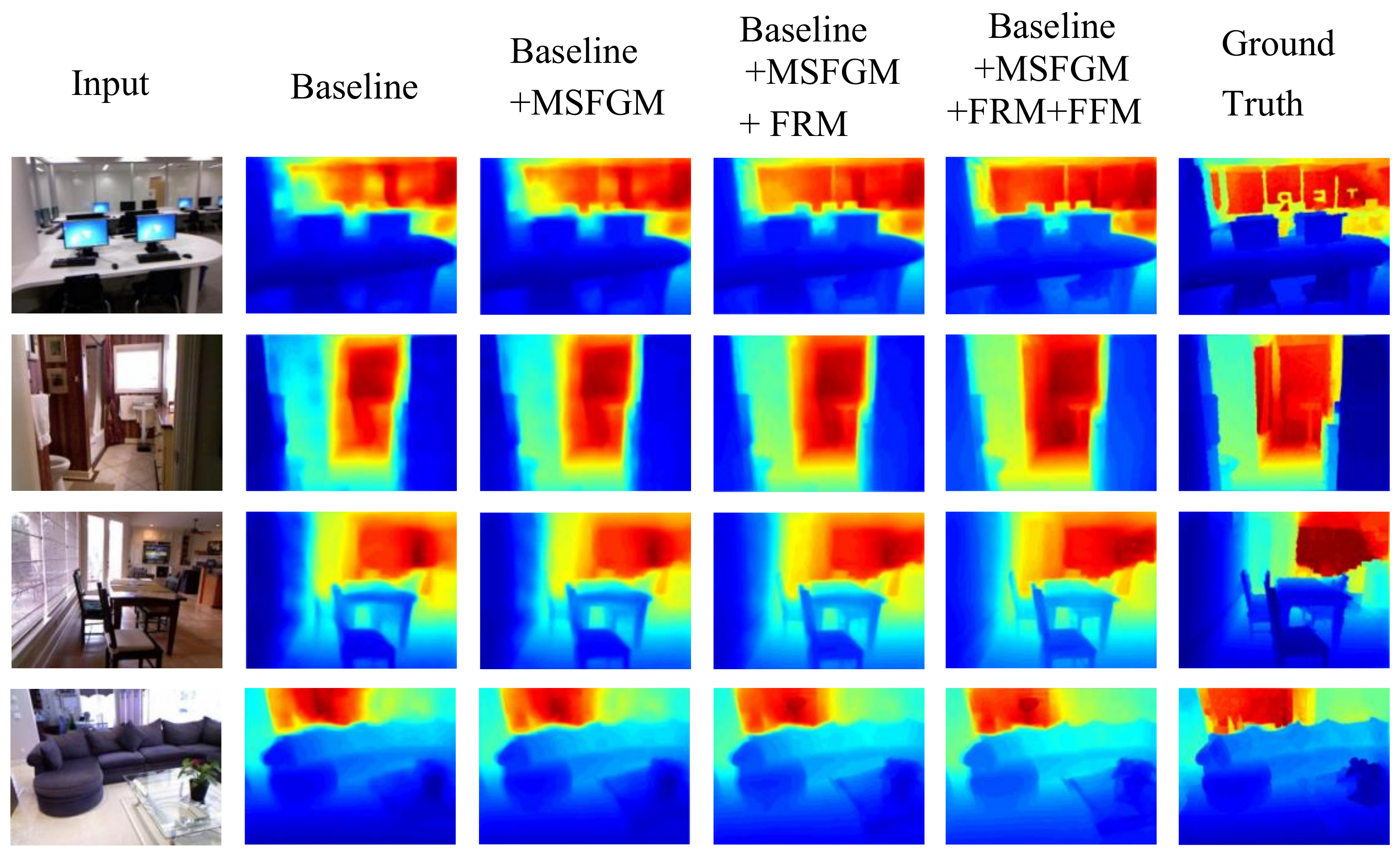
A qualitative evaluation was also performed to compare our approach and other depth reconstruction methods. Figure 6 demonstrates the qualitative comparison results for the NYUv2 dataset, which further verifies the efficiency of our model. The approaches outlined in Refs. [5,21,22,48,50] can obtain precise depth results but have relatively fuzzy edge details. Many fine structures and object edge information are lost, and the depth predictions in some regions have incorrect values. Compared with the results in Ref. [5], the results from Lee et al. [50] provide a relatively accurate 3D structure. However, observing the eighth row and last row in Figure 6, we can see that the results are significantly blurrier than ours and cannot accurately maintain fine details of the scene. As seen from the last row in Figure 6, our method can recover convincing depth maps with clearer edges.

Figure 6. Assessment results for NYUv2 dataset from a qualitative perspective. First row: input, second row: ground truth, third row to last row: depths recovered by Liu et al. [21], Laina et al. [5], Fu et al. [22], Jiang et al. [48], Lee et al. [50] and our method.

For the KITTI dataset, the qualitative results generated from the present work were compared with those of other competitive methods [4,22,55], which are demonstrated in Figure 7. Among them, Eigen et al. [4] is the earliest coarse-to-fine method using convolutional neural networks, whereas Fu et al. [22] applied a depth ordinal regression idea. Alhashim et al. [55] used transfer learning whereas our method designed efficient feature extraction, feature enhancement, and fusion schemes to predict high-quality depths. It can be seen from the results that objects in depth maps recovered by our approach have sharper contours, such as the trees in the second column and the car lights in the first and third columns. Furthermore, our model can obtain more reasonable depth information for distant objects, such as the distant street lights in the second row. Overall, our outputs are closest to the ground-truth depths and achieve attractive performance in both objective and visual comparisons. We also performed a qualitative evaluation between our approach and other depth recovery algorithms, as outlined in this section.

Figure 7. Assessment results for the KITTI dataset from a qualitative perspective. First row: input, second row: sparse ground truth, third row: dense ground truth, fourth row to last row: depths recovered by Eigen et al. [4], Fu et al. [22], Alhashim et al. [55] and our method.

Figure 8 provides the comparison results on the Make3D dataset for methods proposed by Fang et al. [46], Liu et al. [21], Laina et al. [5], Godard et al. [29], Watson et al. [30], and our method. The methods of Godard et al. [29] and Watson et al. [30] belongs to self-supervised learning, whereas other methods are supervised learning. The overall result for Fang et al. [46] is relatively fuzzy and cannot be used to recover accurate depth values for objects at far distances. Here, Liu et al.’s [21] approach and Laina et al’s. [5] approaches outperform Fang et al.’s [46] approach. However, the depth details at the edges are not sufficiently clear. Overall, the structures of the depth results estimated by our method are very similar to those of the real scene since we make full use of spatial features, feature enhancement, and fusion schemes.

Figure 8. Assessment results on the Make3D dataset. First row: input, second row: ground-truth, third row to last row: depths recovered by Fang et al. [58], Liu et al. [21], Laina et al. [5], Godard et al. [29], Watson et al. [30], and our method.

4.3. Ablation Study

We used the NYU v2 dataset to perform ablation experiments to demonstrate the effectiveness of our framework. There are three innovative modules contained in our framework: the multilevel spatial feature generation module (MSFGM), feature refinement module (FRM), and feature fusion module (FFM). The MSFGM is designed for receiving multilevel depth feature maps from the spatial branch. FRM can effectively integrate and enhance the contextual and spatial features, whereas FFM adaptively fuses the fully connected multiscale features. The baseline network contains a backbone network and a decoder (i.e., consecutive upsampling blocks). We gradually added new modules to the baseline network and checked the effectiveness of the added modules according to the evaluation criteria. As reported in Table 4 and Figure 9, the performance of the baseline network is not ideal since it only considers the contextual features of an input color image. After adding MSFGM, the results were slightly better than the baseline. The performance of the model is further improved when FRM is added, which indicates that the feature refinement operation can preserve more depth details. As can be seen from the table, the presented framework realizes the optimal performance when MSFGM, FRM, and FFM are introduced. This demonstrates the effectiveness of methods such as spatial feature extraction, feature refinement, full feature connection, and adaptive fusion. When all modules are combined, we obtain the best depth recovery outputs.

Table 4. Quantitative comparison of MSFGM, FRM, and FFM.

Methods	RMSE(lin)	log10	Rel	δ < 1.25	δ < 1.252	δ < 1.253
Baseline	0.561	0.073	0.163	0.737	0.928	0.990
Baseline + MSFGM	0.552	0.069	0.138	0.743	0.933	0.991
Baseline + MSFGM + FRM	0.498	0.059	0.125	0.806	0.953	0.992
Baseline + MSFGM + FRM + FFM	0.463	0.049	0.115	0.868	0.977	0.993

Figure 9. Depth prediction results for different components.

The definition of the loss function plays an essential role in MDE. To measure the ordinal relationship of the sampled pairs between two depth maps, a new relative loss term was added to the traditional loss function. We then reweighted all the loss terms for multilevel outputs from the decoder part to provide depth details. Table 5 reports the quantitative evaluation results with or without using the relative loss term and the reweight method. The ‘L_berhu + L_gra’ model means our network does not use the relative loss term and the reweight method. ‘L_berhu + L_gra + L_rel’ indicates our network using the Berhu loss, gradient loss, and relative loss terms, whereas ‘L_berhu + L_gra + L_rel + RW’ denotes our network uses the relative loss term and the reweight scheme. When new loss items are added, the RMSE(lin) reaches 0.463, and δ < 1.25 is improved by approximately 0.015. It can be seen that the reweighing strategy contributes to improving the performance of our method. We simultaneously compare the proposed backbone network with two other commonly used backbone networks: VGG19 and ResNet50. To ensure the fairness of the experiments, other modules used in the experiments are the same. The performance comparison of different backbone networks is shown in Table 6. The studied backbone network is designed with ResNet101 on the basis of dilated convolution. The measure values show the effectiveness of the studied backbone network. Compared with VGG19 and ResNet50, the studied backbone network is deeper, and the overall structure and local details of the deep results are better preserved. The running time comparison of different methods on the NYU dataset is shown in Table 7. Since the backbone network of the depth estimation method proposed by Laina et al. [5] is ResNet50, we also replace the backbone network in this study with ResNet50 and give the running time. Due to our designed high-performance encoder and a lightweight decoder with only four up-projection blocks, our method takes less inference time than other methods.

Table 5. Quantitative evaluation results of different loss terms.

Loss Terms	RMSE(lin)	log10	Rel	δ < 1.25	δ < 1.252	δ < 1.253
Lberhu + Lgra	0.483	0.060	0.115	0.853	0.969	0.992
Lberhu + Lgra + Lrel	0.480	0.060	0.116	0.856	0.970	0.993
Lberhu + Lgra + Lrel + RW	0.463	0.049	0.115	0.868	0.977	0.993

Table 6. Quantitative comparison results of different backbone networks.

Backbone	RMSE(lin)	log10	Rel	δ < 1.25	δ < 1.252	δ < 1.253
VGG19	0.615	0.073	0.756	0.936	0.980	VGG19
ResNet50	0.556	0.064	0.809	0.954	0.983	ResNet50
Ours	0.463	0.049	0.868	0.977	0.993	Ours

Table 7. Runtime comparison for different methods on NYU dataset.

Methods	Time (ms)
Eigen [4]	201.3
Liu et al. [21]	175.2
Laina et al. [5]	72.4
Chakrabarti et al. [61]	150.3
Ours (Resnet50)	70.5
Ours	81.3

4.4. Generalization

We used the scene dataset V1 [62] to verify the generalization ability of the method. The images and depths in scene dataset V1 were captured using a Kinect camera. We randomly selected 569 images from the scene V1 database for testing and used the NYU Depth V2 model without fine-tuning as the training model. Figure 10 illustrates the comparison results of depth prediction on scene dataset V1. The first and second columns of Figure 10 present RGB images and the corresponding depths, respectively. The third to last columns of Figure 10 illustrate the depth results estimated by Liu et al. [21], Laina et al. [5], Hu et al. [6], and our method, respectively. Our network obtained a more reasonable depth map with a clearer edge structure. For example, the edges of the table in the second and third rows are clearer than the results obtained using the Liu et al. [21] and Laina et al. [5] methods. The depth details of the bowls in the first row, fourth row, and fifth row are also more convincing. Table 8 outlines the evaluation outputs of depth prediction on scene dataset V1. We tested the pretrained NYU model on scene dataset V1, and the results were significantly different from those directly tested on the NYU test set. Compared to some earlier methods, Hu et al. [6] outperformed Liu et al. [21] and Laina et al. [5]. Compared with methods by Laina et al. [5], Hu et al. [6], and Liu et al. [21], our method performed better for metrics RMSE(lin), Rel, and δ < 1.25³. Thus, the proposed approach delivers comparable performance from a qualitative and quantitative perspective.

Figure 10. Visual comparison on the scene dataset V1. The first column to last column: input, ground truth, depths recovered by Liu et al. [21], Laina et al. [5], Hu et al. [6], and our method.

Table 8. Quantitative evaluation for the scene dataset V1 with the NYU Depth V2 model.

Methods	RMSE(lin)	log10	Rel	δ < 1.25	δ < 1.252	δ < 1.253
Hu et al. [6]	1.551	0.196	0.340	0.179	0.547	0.849
Liu et al. [21]	2.254	0.205	0.356	0.162	0.497	0.816
Laina et al. [5]	1.896	0.200	0.344	0.168	0.531	0.827
Our method	1.449	0.199	0.337	0.173	0.601	0.855

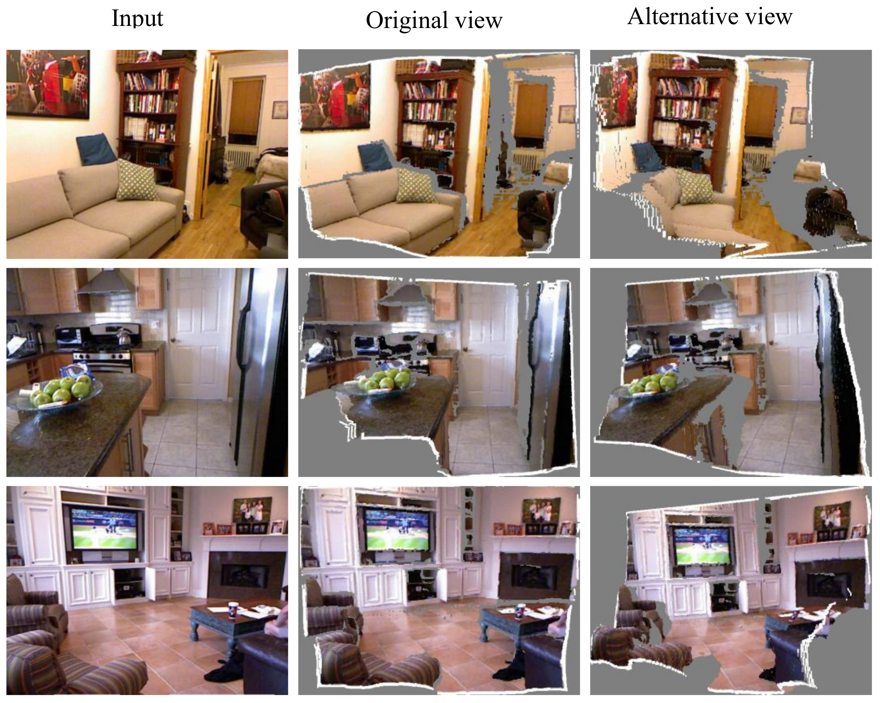
4.5. Application: 3D Reconstruction

We next provide qualitative evaluation results of a 3D reconstruction application to verify the usefulness of our method. The results are displayed in Figure 11. The visual images produced by the presented approach offer a realistic effect compared to those produced by Jiang et al. [48]. Thanks to our multilevel feature extraction module, feature refinement module, feature fusion module and hybrid loss function, the 3D reconstructions obtained by our method are close to the scene structure. Figure 10 denotes reconstruction results from different views by leveraging our method. The 3D comparison results in Figure 12 further prove the effectiveness of our algorithm.

Figure 11. 3D visualization results on the NYU v2 dataset. The first column to last column: input, ground truth, depths recovered by Jiang et al. [48] and our method.

Figure 12. 3D reconstruction results by leveraging our method.

5. Conclusions

For obtaining precise depth maps with rich local details, an efficient multilevel pyramid network for monocular depth prediction on the basis of feature refinement and adaptive fusion has been presented in this study. Unlike most depth estimation algorithms that only acquire contextual features, this study also considers the extraction of spatial features. Specifically, a spatial feature extraction scheme is designed for generating multi-scale information with better edge details. In addition, the feature refinement module is developed to focus on meaningful structural components of the scene, whereas the devised feature fusion module efficiently integrates these significant features for refining depth details. Moreover, we have also designed an efficient hybrid loss function that further considers related relationships and reweighted loss terms to obtain higher-precision depth outputs. The evaluation results for four RGBD datasets demonstrate that our method can obtain precise depths with better details, especially for distant objects and object edges. Nevertheless, our method has some limitations. For instance, it fails to generate depth maps with better details when the depth distributions of test images and training data have little correlation. Thus, in future work, how to combine domain adaptation methods to overcome domain changes is a direction worth exploring.

References

- Yu, S.; Sun, S.; Yan, W.; Liu, G.; Li, X. A Method Based on Curvature and Hierarchical Strategy for Dynamic Point Cloud Compression in Augmented and Virtual Reality System. Sensors 2022, 22, 1262. [Google Scholar] [CrossRef] [PubMed]
- Bertels, M.; Jutzi, B.; Ulrich, M. Automatic Real-Time Pose Estimation of Machinery from Images. Sensors 2022, 22, 2627. [Google Scholar] [CrossRef] [PubMed]
- Nie, X.; Min, C.; Pan, Y.; Li, K.; Li, Z. Deep-neural-network-based modelling of longitudinal-lateral dynamics to predict the vehicle states for autonomous driving. Sensors 2022, 22, 2013. [Google Scholar] [CrossRef]
- Eigen, D.; Fergus, R. Predicting depth, surface normals and semantic labels with a common multi-scale convolutional architecture. In Proceedings of the IEEE International Conference on Computer Vision, Santiago, Chile, 13–16 December 2015; pp. 2650–2658. [Google Scholar]
- Laina, I.; Rupprecht, C.; Belagiannis, V.; Tombari, F.; Navab, N. Deeper depth prediction with fully convolutional residual networks. In Proceedings of the International Conference on 3D Vision, Stanford, CA, USA, 25–28 October 2016; pp. 239–248. [Google Scholar]
- Hu, J.; Ozay, M.; Zhang, Y.; Okatani, T. Revisiting single image depth estimation: Toward higher resolution maps with accurate object boundaries. In Proceedings of the 2019 IEEE Winter Conference on Applications of Computer Vision (WACV), Waikoloa, HI, USA, 7–11 January 2019; pp. 1043–1051. [Google Scholar]
- Su, W.; Zhang, H.; Su, Y. Monocular depth estimation with spatially coherent sliced network. Image Vis. Comput. 2022, 124, 104487. [Google Scholar] [CrossRef]
- Tao, B.; Chen, X.; Tong, X. Self-Supervised Monocular Depth Estimation Based on Channel Attention. Photonics 2022, 9, 434. [Google Scholar] [CrossRef]
- Kim, D.; Ga, W.; Ahn, P. Global-Local Path Networks for Monocular Depth Estimation with Vertical CutDepth. arXiv 2022, arXiv:2201.07436. [Google Scholar]
- Swami, K.; Muduli, A.; Gurram, U. Do What You Can, with What You Have: Scale-Aware and High Quality Monocular Depth Estimation without Real World Labels. In Proceedings of the IEEE/CVF Conference on Computer Vision and Pattern Recognition, New Orleans, LA, USA, 19–24 June 2022; pp. 988–997. [Google Scholar]
- Ma, H.; Ding, Y.; Wang, L. Depth Estimation from Monocular Images Using Dilated Convolution and Uncertainty Learning. In Proceedings of the Pacific Rim Conference on Multimedia, Hefei, China, 21–22 September 2018; pp. 13–23. [Google Scholar]
- Petrovai, A.; Nedevschi, S. Exploiting Pseudo Labels in a Self-Supervised Learning Framework for Improved Monocular Depth Estimation. In Proceedings of the IEEE/CVF Conference on Computer Vision and Pattern Recognition, New Orleans, LA, USA, 19–24 June 2022; pp. 1578–1588. [Google Scholar]
- Wang, X.; Fu, X.; Dong, Q. Image Depth Estimation Model Based on Fully Convolutional U-Net. Comput. Sci. Appl. 2019, 9, 250–255. [Google Scholar]
- Xu, H.; Li, F.; Feng, Z. MLFFNet: Multilevel feature fusion network for monocular depth estimation from aerial images. J. Appl. Remote Sens. 2022, 16, 026506. [Google Scholar] [CrossRef]
- Sagar, A. Monocular depth estimation using multi scale neural network and feature fusion. In Proceedings of the IEEE/CVF Winter Conference on Applications of Computer Vision Workshops (WACVW), Waikoloa, HI, USA, 4–8 January 2022; pp. 656–662. [Google Scholar]
- Agarwal, A.; Arora, C. Depthformer: Multiscale Vision Transformer for Monocular Depth Estimation with Local Global Information Fusion. arXiv 2022, arXiv:2207.04535. [Google Scholar]
- Ye, X.; Chen, S.; Xu, R. DPNet: Detail-preserving network for high-quality monocular depth estimation. Pattern Recognit. 2021, 109, 107578. [Google Scholar] [CrossRef]
- Pei, M. MSFNet: Multi-scale features network for monocular depth estimation. arXiv 2021, arXiv:2107.06445. [Google Scholar]
- Chen, Y.; Zhao, H.; Hu, Z.; Peng, J. Attention-based context aggregation network for monocular depth estimation. Int. J. Mach. Learn. Cybern. 2021, 12, 1583–1596. [Google Scholar] [CrossRef]
- Wei, J.; Pan, S.; Gao, W. Triaxial Squeeze Attention Module and Mutual-Exclusion Loss Based Unsupervised Monocular Depth Estimation. Neural Process. Lett. 2022, 1–16. [Google Scholar] [CrossRef]
- Liu, F.; Shen, C.; Lin, G.; Reid, I. Learning depth from single monocular images using deep convolutional neural fields. IEEE Trans. Pattern Anal. Mach. Intell. 2016, 38, 2024–2039. [Google Scholar] [CrossRef] [Green Version]
- Fu, H.; Gong, M.; Wang, C.; Batmanghelich, K.; Tao, D. Deep ordinal regression network for monocular depth estimation. In Proceedings of the IEEE Conference on Computer Vision and Pattern Recognition, Salt Lake City, UT, USA, 18–22 June 2018; pp. 2002–2011. [Google Scholar]
- Song, M.; Lim, S.; Kim, W. Monocular Depth Estimation Using Laplacian Pyramid-Based Depth Residuals. IEEE Trans. Circuits Syst. Video Technol. 2021, 31, 4381–4393. [Google Scholar] [CrossRef]
- Wu, J.; Ji, R.; Wang, Q. Fast Monocular Depth Estimation via Side Prediction Aggregation with Continuous Spatial Refinement. IEEE Trans. Multimed. 2022. [Google Scholar] [CrossRef]
- Gao, T.; Wei, W.; Cai, Z. CI-Net: A joint depth estimation and semantic segmentation network using contextual information. Appl. Intell. 2022, 1–20. [Google Scholar] [CrossRef]
- Zhao, X.; Pang, Y.; Zhang, L. Joint Learning of Salient Object Detection, Depth Estimation and Contour Extraction. arXiv 2022, arXiv:2203.04895. [Google Scholar]
- Wang, Y.; Zhu, H.; Liu, M. CNNapsule: A Lightweight Network with Fusion Features for Monocular Depth Estimation. In Proceedings of the International Conference on Artificial Neural Networks, Bratislava, Slovakia, 14–17 September 2021; pp. 507–518. [Google Scholar]
- Liu, S.; Yang, L.T.; Tu, X. Lightweight Monocular Depth Estimation on Edge Devices. IEEE Internet Things J. 2022. [Google Scholar] [CrossRef]
- Godard, C.; Mac Aodha, O.; Firman, M. Digging into self-supervised monocular depth estimation. In Proceedings of the IEEE/CVF International Conference on Computer Vision, Seoul, Korea, 27 October–2 November 2019; pp. 3828–3838. [Google Scholar]
- Watson, J.; Firman, M.; Brostow, G.J. Self-supervised monocular depth hints. In Proceedings of the IEEE/CVF International Conference on Computer Vision, Seoul, Korea, 27 October–2 November 2019; pp. 2162–2171. [Google Scholar]
- Wong, A.; Soatto, S. Bilateral cyclic constraint and adaptive regularization for unsupervised monocular depth prediction. In Proceedings of the IEEE/CVF Conference on Computer Vision and Pattern Recognition, Long Beach, CA, USA, 16–20 June 2019; pp. 5644–5653. [Google Scholar]
- Tosi, F.; Aleotti, F.; Poggi, M.; Mattoccia, S. Learning monocular depth estimation infusing traditional stereo knowledge. In Proceedings of the IEEE/CVF Conference on Computer Vision and Pattern Recognition, Long Beach, CA, USA, 16–20 June 2019; pp. 9799–9809. [Google Scholar]
- Ling, C.; Zhang, X.; Chen, H. Unsupervised Monocular Depth Estimation using Attention and Multi-Warp Reconstruction. IEEE Trans. Multimed. 2021, 24, 2938–2949. [Google Scholar] [CrossRef]
- Ye, X.; Fan, X.; Zhang, M.; Xu, R.; Zhong, W. Unsupervised Monocular Depth Estimation via Recursive Stereo Distillation. IEEE Trans. Image Process. 2021, 30, 4492–4504. [Google Scholar] [CrossRef] [PubMed]
- Sun, Q.; Tang, Y.; Zhang, C.; Zhao, C.; Qian, F.; Kurths, J. Unsupervised Estimation of Monocular Depth and VO in Dynamic Environments via Hybrid Masks. IEEE Trans. Neural Netw. Learn. Syst. 2021, 33, 2023–2033. [Google Scholar] [CrossRef] [PubMed]
- Chiu, M.-J.; Chiu, W.C.; Chen, H.T.; Chuang, J.H. Real-time Monocular Depth Estimation with Extremely Light-Weight Neural Network. In Proceedings of the 2020 25th International Conference on Pattern Recognition (ICPR), Milan, Italy, 10–15 January 2021. [Google Scholar]
- Varma, A.; Chawla, H.; Zonooz, B.; Arani, E. Transformers in Self-Supervised Monocular Depth Estimation with Unknown Camera Intrinsics. arXiv 2022, arXiv:2202.03131. [Google Scholar]
- Yang, J.; An, L.; Dixit, A. Depth Estimation with Simplified Transformer. arXiv 2022, arXiv:2204.13791. [Google Scholar]
- Mendoza, J.; Pedrini, H. Self-distilled Self-supervised Depth Estimation in Monocular Videos. In Proceedings of the International Conference on Pattern Recognition and Artificial Intelligence, Chengdu, China, 19–21 August 2022; pp. 423–434. [Google Scholar]
- Fu, J.; Liu, J.; Tian, H. Dual attention network for scene segmentation. In Proceedings of the IEEE/CVF conference on computer vision and pattern recognition, Long Beach, CA, USA, 15–20 June 2019; pp. 3146–3154. [Google Scholar]
- Zhang, L.; Zhang, L.; Mou, X.; Zhang, D. FSIM: A feature similarity index for image quality assessment. IEEE Trans. Image Process. 2011, 20, 2378–2386. [Google Scholar] [CrossRef] [Green Version]
- Chen, T.; An, S.; Zhang, Y.; Ma, C.; Wang, H.; Guo, X.; Zheng, W. Improving monocular depth estimation by leveraging structural awareness and complementary datasets. In Proceedings of the European Conference on Computer Vision, Online, 23–28 August 2020; pp. 90–108. [Google Scholar]
- Silberman, N.; Hoiem, D.; Kohli, P.; Fergus, R. Indoor segmentation and support inference from rgbd images. In Proceedings of the European Conference on Computer Vision, Firenze, Italy, 7–13 October 2012; pp. 746–760. [Google Scholar]
- Geiger, A.; Lenz, P.; Stiller, C.; Urtasun, R. Vision meets robotics The KITTI dataset. Int. J. Robot. Res. 2013, 32, 1231–1237. [Google Scholar] [CrossRef] [Green Version]
- Carvalho, M.; Le Saux, B.; Trouvé-Peloux, P.; Almansa, A.; Champagnat, F. On regression losses for deep depth estimation. In Proceedings of the 2018 25th IEEE International Conference on Image Processing, Athens, Greece, 7–10 October 2018; pp. 2915–2919. [Google Scholar]
- Moukari, M.; Picard, S.; Simon, L.; Jurie, F. Deep multi-scale architectures for monocular depth estimation. In Proceedings of the 2018 25th IEEE International Conference on Image Processing, Athens, Greece, 7–10 October 2018; pp. 2940–2944. [Google Scholar]
- Xu, D.; Ricci, E.; Ouyang, W.; Wang, X.; Sebe, N. Multi-scale continuous crfs as sequential deep networks for monocular depth estimation. In Proceedings of the IEEE Conference on Computer Vision and Pattern Recognition, Honolulu, HI, USA, 21–26 July 2017; pp. 5354–5362. [Google Scholar]
- Jiang, H.; Huang, R. High quality monocular depth estimation via a multi-scale network and a detail-preserving objective. In Proceedings of the 2019 IEEE International Conference on Image Processing (ICIP), Taipei, Taiwan, 22–25 September 2019. [Google Scholar]
- Wang, L.; Zhang, J.; Wang, O.; Lin, Z.; Lu, H. Sdc-depth: Semantic divide-and-conquer network for monocular depth estimation. In Proceedings of the IEEE/CVF Conference on Computer Vision and Pattern Recognition, Seattle, WA, USA, 14–19 June 2020; pp. 541–550. [Google Scholar]
- Lee, J.H.; Kim, C.S. Monocular depth estimation using relative depth maps. In Proceedings of the IEEE/CVF Conference on Computer Vision and Pattern Recognition, Long Beach, CA, USA, 16–20 June 2019; pp. 9729–9738. [Google Scholar]
- Ramamonjisoa, M.; Lepetit, V. Sharpnet: Fast and accurate recovery of occluding contours in monocular depth estimation. In Proceedings of the IEEE/CVF International Conference on Computer Vision Workshops, Seoul, Korea, 27–28 October 2019. [Google Scholar]
- Liu, P.; Zhang, Z.H.; Meng, H.; Gao, N. Joint attention mechanisms for monocular depth estimation with multi-scale convolutions and adaptive weight adjustment. IEEE Access 2020, 8, 184437–184450. [Google Scholar] [CrossRef]
- Liu, J.; Zhang, Y.; Cui, J.; Feng, Y.; Pang, L. Fully convolutional multi-scale dense networks for monocular depth estimation. IET Comput. Vis. 2019, 13, 515–522. [Google Scholar] [CrossRef]
- Fang, Z.; Chen, X.; Chen, Y.; Gool, L.V. Towards good practice for CNN-based monocular depth estimation. In Proceedings of the IEEE/CVF Winter Conference on Applications of Computer Vision, Snowmass Village, CO, USA, 2–5 March 2020; pp. 1091–1100. [Google Scholar]
- Alhashim, I.; Wonka, P. High quality monocular depth estimation via transfer learning. arXiv 2018, arXiv:1812.11941. [Google Scholar]
- Chen, S.; Fan, X.; Pu, Z.; Ouyang, J.; Zou, B. Single image depth estimation based on sculpture strategy. Knowl. Based Syst. 2022, 250, 109067. [Google Scholar] [CrossRef]
- Gan, Y.; Xu, X.; Sun, W.; Lin, L. Monocular depth estimation with affinity, vertical pooling, and label enhancement. In Proceedings of the European Conference on Computer Vision, Munich, Germany, 8–14 September 2018; pp. 232–247. [Google Scholar]
- Fang, S.; Jin, R.; Cao, Y. Fast depth estimation from single image using structured forest. In Proceedings of the 2016 IEEE International Conference on Image Processing (ICIP), Phoenix, AZ, USA, 25–28 September 2016; pp. 4022–4026. [Google Scholar]
- Kim, Y.; Jung, H.; Min, D.; Sohn, K. Deep monocular depth estimation via integration of global and local predictions. IEEE Trans. Image Process. 2018, 27, 4131–4144. [Google Scholar] [CrossRef] [PubMed]
- Kuznietsov, Y.; Stuckler, J.; Leibe, B. Semisupervised deep learning for monocular depth map prediction. In Proceedings of the IEEE Conference on Computer Vision Pattern Recognition, Honolulu, HI, USA, 21–26 July 2017; pp. 2215–2223. [Google Scholar]
- Chakrabarti, S.A.; Shakhnarovich, J.G. Depth from a single image by harmonizing overcomplete local network predictions. arXiv 2016, arXiv:1605.0708. [Google Scholar]
- Lai, K.; Bo, L.; Ren, X.; Fox, D. A large-scale hierarchical multi-view rgb-d object dataset. In Proceedings of the 2011 IEEE International Conference on Robotics and Automation, Shanghai, China, 9–13 May 2011; pp. 1817–1824. [Google Scholar]
Publisher’s Note: MDPI stays neutral with regard to jurisdictional claims in published maps and institutional affiliations. |
© 2022 by the authors. Licensee MDPI, Basel, Switzerland. This article is an open access article distributed under the terms and conditions of the Creative Commons Attribution (CC BY) license (https://creativecommons.org/licenses/by/4.0/).