Big-Data Platform for Performance Monitoring of Telecom-Service-Provider Networks

Abstract

Large telecom-service-provider networks are typically based on complex communications infrastructures comprising millions of network devices. The performance monitoring of such networks is a very demanding and challenging task. A large amount of data is collected and processed during performance monitoring to obtain information that gives insights into the current network performance. Using the obtained information, providers can efficiently detect, locate, and troubleshoot weak spots in the network and improve the overall network performance. Furthermore, the extracted information can be used for planning future network expansions and to support the determination of business-strategy decisions. However, traditional methods for processing and storing data are not applicable because of the enormous amount of collected data. Thus, big-data technologies must be used. In this paper, a big-data platform for the performance monitoring of telecom-service-provider networks is proposed. The proposed platform is capable of collecting, storing, and processing data from millions of devices. Typical challenges and problems in the development and deployment process of the platform, as well as the solutions to overcome them, are presented. The proposed platform is adjusted to HFC (Hybrid Fiber-Coaxial) network and currently operates in the real HFC network, comprising millions of users and devices.

1. Introduction

Large telecom service providers provide services to millions of users using large, heterogeneous, and continuously evolving network infrastructure. Keeping subscribers satisfied is very important for telecom service providers. Thus, network performance is a key aspect for service providers. In order to keep network performance at a high level, providers must collect and process data from network devices to obtain relevant information (the detection of traffic bottlenecks, the detection of poor-performance devices, etc.). Furthermore, telecom service providers, based on the obtained information, can efficiently plan future network expansions, such as installing higher-capacity links in congested parts of the network, offering new services to users, equipment acquisition planning, etc.

The amount of collected data is enormous given the large number of network devices and the need for continuous data collection. Traditional methods for the storage and processing of large data sets are practically useless due to the limited resources and lack of scalability [1]. Only small data subsets are processed because a significant amount of collected data is discarded due to hardware and computing limitations. Big-data technologies are introduced to overcome these limitations [1,2]. There are many definitions of the term, big data [2]. In general, all definitions of big data relate to amounts of data that are not manageable using traditional processing systems and/or cannot be stored in traditional data warehouses.

Big-data technologies are used by telecom service providers for network-performance monitoring. Providers use either commercially available (e.g., SolarWinds NPM, ManageEngine OpManager) or custom-based big-data solutions. However, there is a research gap in the literature regarding the detailed specifications and explanations of the overall big-data architectures used in real telecom operator networks. Furthermore, deployment experiences that can be very valuable are mostly missing in the available literature. Thus, our motivation is to fill this research gap by proposing a scalable and flexible big-data architecture for telecom-service-provider network-performance monitoring, which is explained in detail, along with our deployment experiences.

In this paper, we consider the HFC (Hybrid Fiber-Coaxial) network as a telecom-service-provider network. HFC technology is a result of the CATV (cable television) evolution [3]. CATV operators replaced large portions of their all-coaxial planes with fiber to increase system capacity. CATV networks modified in such a way are known as HFC networks. Currently, HFC networks provide extremely wide bandwidth to their users. Additionally, HFC networks extend their functionality to deliver so-called “triple-play service” (television, broadband internet access, and IP telephony) [4].

We propose a novel big-data platform for the performance monitoring (BDPfPM) of telecom-service-provider networks based on open-source big-data tools. The proposed BDPfPM is deployed and currently successfully operates in a real HFC network, comprising millions of devices and users. BDPfPM is designed to be flexible and scalable. Thus, BDPfPM can be adjusted to other large communications networks, and to other industries that have similar monitoring challenges, such as the IoT (Internet of Things), smart cities, smart grids, etc. The contributions of the paper are:

• A developed BDPfPM for telecom-service-provider networks that is successfully deployed in a real HFC network, comprising millions of devices and users;
• A description of the requirements, challenges, and solutions analysis involved in introducing and deploying BDPfPM in telecom-service-provider HFC networks, including a novel data schema for faster queries;
• The detection of weak spots in the network.

The rest of the paper is organized as follows. In Section 2, we give an overview of the related work. In Section 3, we briefly present the HFC network architecture, since BDPfPM is deployed in a real HFC network. In Section 4, a discussion regarding the BDPfPM design objectives and challenges is given. Section 5 presents the proposed BDPfPM. In this section, we describe all the BDPfPM components and functions in detail. Section 6 presents a performance estimation of devices in the network used for detection of poor-performance devices, i.e., weak spots in the network. In Section 7, we present the challenges that emerged during the BDPfPM deployment and the solutions proposed to overcome these challenges. Section 8 concludes the paper and gives the directions of future work.

2. Related Work

Big data is a major topic in various applications, such as smart grids [5], healthcare [6], IoT [7], etc. However, different applications face different big-data challenges. For example, some applications focus on storage and data aggregation [8,9], other applications focus on real-time and event processing [10,11], while some applications focus on efficient search [12], etc. In this section, we give a brief overview of related work relevant to the proposed BDPfPM.

An overview of big-data technologies is given in [13]. The Apache foundation is introduced and the main tools from the Hadoop family are presented. Additionally, different distributions of big-data systems are presented, along with an analysis of on-premises and cloud implementations. Furthermore, an analysis of big-data applications in different industries is provided. Finally, the challenges that big data technologies currently face are presented. Cloud computing in big data solutions is an attractive topic that receives special attention in the literature [14,15]. A survey on big data and cloud computing is given in [16], while the data-security aspects in the big-data cloud computing environment are discussed in [17].

Atat et al. give a detailed panoramic survey of big-data applications in cyber-physical systems [18]. An analysis of the available research related to big data and cyber-physical systems is provided. The analysis covers all the layers of end-to-end big-data systems, a variety of data sources and collections, caching and routing, an overview of available tools and systems, security, environmental problems, current challenges, and open issues.

Jiang et al. focus on the big-data technologies in the energy industry [19]. An appropriate integrated big-data architecture is proposed for the smart grid. Furthermore, each layer of the proposed architecture is analyzed in detail.

Given the large number of customers and devices in the network, big data is very appealing to telecom service providers for improving business results and customer satisfaction. The application of big data in mobile networks is described in [20]. Big data is defined mathematically through random matrices, after which it is connected to the data from mobile networks. Furthermore, cellular networks and the presence of big data in them are explained in detail. Liu et al. propose a Hadoop-based network monitoring and analysis system for big traffic data [21]. The system is designed as a multi-layer architecture. Finally, the system is implemented in the core of 2G and 3G cellular networks with an appropriate demonstration of the results. Akbar et al. discuss the application of machine learning and complex-event processing through data streaming [22]. Using these technologies, a solution for traffic-congestion prediction is proposed. The authors connect several data sources and create decision rules. A traffic-jam prediction is performed based on the trained model.

Benhavan et al. [3] analyze quality monitoring in HFC networks. Additionally, they propose a special method for performance analysis. The method is based on three-dimensional analysis using data from CMTSs (Cable Modem Termination Systems) and cable modems. In [23], all the challenges for performance management in HFC networks are summarized. Furthermore, a list of the most important performance metrics for cable modems and CMTSs is proposed.

Big-data systems often need to analyze and process time-series data, similarly to the BDPfPM proposed in this paper. Rafferty et al. propose a solution for storing time-series sensor data [24]. The solution is a scalable, modular platform for storing sensor measurements. For communication with the sensor, a MQTT (Message-Queuing Telemetry Transport) protocol is proposed, together with REST (Representational State Transfer) and web socket. InfluxDB is used as the platform core. Wang et al. apply machine learning on time-series data [25]. They propose the application of several different machine-learning models to a stock-trading data set for specific scenarios.

Although BDPfPM is focused on batch-data processing, streaming-data processing is another very important method. Streaming-data processing is even more challenging because data need to be collected and processed in real time, and data generation can be very fast [26]. In fact, some of the most challenging problems belong to the streaming data processing such as repairing and cleaning data in real-time [27], the extraction of metadata [28], and online data representation [29]. In [30], popular stream-processing frameworks, such as Flink, Kafka, and Spark are compared.

Wu et al. investigate the impact of big-data processing on the environment and try to correlate the two [31]. The impact is analyzed through the whole lifecycle of data processing. The authors analyze metrics related to this topic and suggest new metrics.

Big data is used in many monitoring systems, such as weather monitoring [32], biogas-detection-monitoring systems [33], the Internet of Vehicles [34], etc. Since monitoring systems often deploy sensors for monitoring purposes, IoT-monitoring systems are very common. Typically, these systems deploy simple hardware, such as Arduino, for data collection from sensors, and the collected data are sent to a centralized big-data platform [32,33]. The Internet of Vehicles (IoV) is an important and emerging area, in which monitoring is a crucial component given the safety requirements. Furthermore, real-time and low-latency data collection and processing are mandatory for such networks [34]. The IoV might require distributed big-data architecture, in which some of the processing is placed in fog closer to data sources and consumers to reduce the latency.

Regarding network-performance monitoring, network traffic can be used as a data source [35]. However, this approach might be impractical for large networks and core networks that install high-capacity links (100 Gbps and beyond). However, for small networks, this approach could be useful, especially for detecting malicious traffic and intrusion attempts. A big-data framework for performance management in mobile networks is proposed in [36]. The proposed framework architecture uses the HDFS file system and focuses on batch processing. The data from the data sources are collected in the XML format and Flume is used for data collection. The framework is tested on 5G data sets. Data replication is used to simulate the generation of performance-management files to test the framework. The framework proposed in [36] has a similar approach to our proposed BDPfPM; however, it is tested on simulated data sets, unlike BDPfPM, which is verified by successfully operating in a real HFC network. Furthermore, deployment in real networks is always accompanied by unpredictable challenges. The deployment of BDPfPM in a real HFC network provided us with experience with some initially unpredicted challenges. These are presented in this paper, along with their solutions.

3. HFC Network Architecture

Since BDPfPM is adjusted to the HFC network, we give a brief overview of the HFC network architecture in this section to define typical devices and their role and position in the HFC network. This brief overview of the HFC network architecture is also important from a big-data point of view because it is not possible to collect data from all the types of devices in the HFC network. For example, it is not possible to collect data from ONs (optical nodes), AMPs (amplifiers), and APs (access points). Thus, it is very important to have HFC network architecture and topology knowledge that can be combined with information obtained from big-data processing to indirectly estimate the state of such devices (ONs, AMPs, and APs).

Figure 1 shows a typical HFC network architecture. In the downstream direction, the regional head-end (CMTS) receives services (TV signal, telephony, and data) and modulates and combines them into a single signal that is distributed via fiber [23]. The optical signal reaches the ON via the Hub. The ON converts the optical signal to the electrical signal and distributes it to the CN (cable network). The CN is a tree-based topology comprising AMPs and splitters. AMPs are used to overcome the coaxial cable attenuation of the electrical signals. Finally, the signal reaches the end-user through the AP and ends in the CPE (customer premises equipment), which can be a CM (cable modem), STB (set-top box), or VoIP (voice over IP) phone. In the opposite (upstream) direction, signals are frequency-division multiplexed, sent over the CN to the ON, converted into the optical signal, and sent back to the CMTS [23].

High-speed broadband services using the HFC cable infrastructure are standardized by DOCSIS (data-over-cable-service interface specification). From the initial cable broadband technology (DOCSIS 1.0) through the VoIP service (DOCSIS 1.1), high throughputs, and multichannel support, the DOCSIS standard has grown into a full-duplex communication system with a capacity of 10 Gbps (DOCSIS 3.1 full-duplex) [23].

4. Objectives and Challenges of BPDfPM

To develop an efficient big-data platform for specific applications, the objectives of the big-data platform must be defined. The analysis of the challenges involved in fulfilling these objectives is also important, as it helps to properly address challenges during big-data-platform development. Therefore, this section is dedicated to defining the objectives of BDPfPM (Section 4.1), as well as to analyzing the big-data challenges from a BDPfPM perspective (Section 4.2).

4.1. BDPfPM Objectives

One of the main objectives of BDPfPM is to establish a centralized performance-monitoring platform. BDPfPM needs to periodically collect and store data from monitored devices (data sources). This type of data is called time series. BDPfPM needs to be capable of collecting data from a huge amount of data sources, which are theoretically infinite in number (in practice, hundreds of billions). In general, there is no regulation regarding data collection period; thus, the collection period depends on the operator policy. Depending on the importance of the collected data (performance metrics in the case of BDPfPM), the typical collection period is in the range of 1 min to 1 h. However, the data access and resolution for a particular monitored device in the case of troubleshooting needs to be in the order of a second. Thus, BDPfPM must be capable of supporting data collection within a period of one second. The retention period for the collected data can differ. BDPfPM needs to be scalable and easily extendable in terms of future extensions, integration with new domains, and the addition of new devices. Furthermore, BDPfPM needs to be based on open-source tools to maximize its cost-effectiveness. Finally, BDPfPM must be highly available.

The primary use of collected data is performance monitoring. In performance monitoring, the collected data are used in reports to observe the current status of a particular segment of the network, as well as its history. The important objective is that the supported network segment be within range of the CPE equipment up to the company level. In this way, network operators are able to detect problematic parts of the network and efficiently plan future network upgrades and expansions.

BDPfPM is adjusted to the HFC network. Therefore, performance statistics are collected from CMTSs and CPEs. One CMTS can serve thousands of subscribers, depending on its type and configuration. For example, the Cisco uBR10000 Series can support up to 64,000 subscribers [37]. Usually, one HFC network operator has tens or even hundreds of CMTSs, depending on the number of subscribers, defined throughput, and configuration. Naturally, there are significantly more CPEs than CMTSs in the HFC network. For example, according to [38], at the end of 2018 Unitymedia had 6,283,000 video and 3,615,500 internet subscribers. Because both CM and STB are CPE, and given that the average subscriber has both, the number of end devices to monitor is approximately twice the number of the subscribers. In [23], a list of the most important performance metrics for the HFC network is proposed. The list contains metrics for both CMTS and CPE. BDPfPM needs to be able to collect and process such performance metrics from an enormous number of devices.

4.2. BDPfPM Challenges

Big-data challenges are typically analyzed using the 5V concept [9]. The 5V concept comprises Volume, Variety, Velocity, Veracity, and Value challenges. In this section, we present the big-data challenges for BDPfPM from the 5V perspective.

Volume challenge relates to enormous amounts of collected data. This challenge is obvious in the case of BDPfPM, given the large number of devices in the HFC network. For example, let us assume that there are one million CPEs in the HFC network, and data are collected once per hour from each CPE. If, on average, every CPE is connected to two streams, then two million rows are collected every hour for only one iteration and only one metric. If BDPfPM were to need to store collected data for the last six months, then around 8.73 billion rows would be stored for only one KPI (key performance indicator). The KPI, or performance metric, is a measurable value that describes the condition of a monitored device. This simple example demonstrates the Volume challenge in the performance monitoring of the HFC network [23].

Obviously, the storage of collected data represents a serious volume challenge in the case of BDPfPM. Considering the amount of collected data that need to be stored and the nature of time-series data, relational databases are not able to satisfy capacity and scalability requirements. Thus, non-relational distributed databases need to be used. Furthermore, query performance is a significant factor in the selection of appropriate storage solution. Moreover, storage based on open-source technologies is preferable. Even when the optimal database is selected, there is still the question of how to store data and gain maximal performance on the device level.

Variety challenge relates to structured and unstructured data that are gathered from multiple data sources. BDPfPM collects data from devices in the HFC network. There are various types of devices in the HFC network. Furthermore, these devices are typically from different vendors (for example, the CMTS vendors include Cisco, CASA, ARRIS, Motorola, Huawei, etc.). Furthermore, even devices from the same vendor can differ. For example, they can have different software versions or different capabilities (e.g., Cisco uBR, cBR, and Remote PHY). The types of collected data differ, depending on the role and capabilities of the device. For example, modems with embedded WiFi, in comparison to modems without WiFi, have metrics associated withWiFi functionality. Furthermore, multiple protocols exist for communication with the monitored devices in the network. The SNMP (Simple Network-Management Protocol), IPDR (Internet Protocol Detail Record), and FTP (File Transfer Protocol) are mostly used for this purpose. However, which protocols can be used depend on the set of protocols supported by the monitored devices. Moreover, BDPfPM should also be capable of receiving data from external sources (external data sources, third-party applications), which increases the variety of collected data. The great aforementioned diversity of devices as data sources represents the Variety challenge in the performance monitoring of the HFC network.

Velocity challenge relates to the generation speed of data. Data collection at higher frequency provides better granularity and insight into HFC network performance, but it requires larger storage resources and processing capabilities due to the greater amount of collected data. A trade-off between the data-collection frequency and the amount of processing and storage resources is always necessary. BDPfPM should be able to allow a temporary collection frequency increase for a particular device to troubleshoot the device’s suspicious behavior. The described Velocity challenge requires the careful selection of data-collection frequency in BDPfPM to achieve an optimal balance between the required storage and processing resources and the quality of information obtained from the collected data.

The data-collection process is a very significant challenge for BDPfPM because it has a major impact on the overall BDPfPM performance. In fact, the data-collection challenge is a combination of the Volume, Variety, and Velocity challenges. The collection layer requires a significant amount of resources given the fact that there the HFC network features a huge number and variety of monitored devices (Volume and Variety challenges). The higher the data collection frequency, the more resources are required (Velocity challenge). The fact that customer equipment is not highly available and can be unreachable for any reason (such as a customer turning off a modem, power outages, the absence of a network connection) additionally increases data-collection times. Furthermore, the range of IP addresses associated with CPEs is dynamic. Custom mechanisms need to be defined to create and maintain mapping between end-user devices and the IP addresses associated with them.

Veracity challenge relates to data confidence, i.e., whether the collected data can be trusted. If data are missing, the cause is uncertain. For example, the cause can be device malfunction, inaccessibility (power loss, connectivity loss), or collector unavailability. Furthermore, there is also uncertainty regarding the accuracy of collected data. Practice has shown that situations leading to inaccurate data can arise. For example, if a telecom service provider reconfigures a device without notifying the BDPfPM, inaccurate data might be collected from the reconfigured device.

Value challenge relates to the ability to transform the vast amount of collected data into useful information. Once data are collected, they are processed to obtain valuable information. Collected data might contain valuable information that is not obvious at first glance. Therefore, big-data platform developers need to understand collected data to be able to define the form of processing that extracts the most valuable information. Based on this understanding, proper data aggregations can be created that extract information (value) from collected data. Data aggregations in BDPfPM are discussed in more detail in Section 5.5.

The HFC network comprises a variety of network devices, as discussed under the Variety challenge section. These devices can be grouped into intelligent (those that can measure and send performance metrics) and non-intelligent. Devices such as ON, AMP, and AP are not able to provide information about their condition. However, if the HFC network topology is known, the data collected from CPEs can be used to estimate the condition of non-intelligent devices. Network topology information needs to be correlated with the data collected from CPEs to estimate the condition of non-intelligent devices. The Value challenge is how to combine collected data with the network topology information to make the best estimation. Note that, given the number of end devices, this is very challenging in terms of processing power. A solution to this Value challenge (estimation of non-intelligent devices) is presented in Section 6.

5. Big-Data Platform for Performance Monitoring

In this section, we give a detailed description of the proposed and implemented BDPfPM. Big-data technologies comprise several software tools. Thus, in Section 5.1, we give a description of the big-data tools used in BDPfPM. The architecture of BDPfPM is presented in Section 5.2, along with a detailed description of all its components. The proposed data schema is explained in Section 5.3. The collection layer is introduced in Section 5.4. Methods for data aggregation are proposed in Section 5.5.

5.1. Big-Data Tools

Big data is a collection of different software tools based on the same distributed principle. These software tools are interdependent and, jointly, they represent a big-data solution. Such a rich portfolio is a response to market requirements for solving specific types of big data problems. BDPfPM uses several open-source big-data tools. In this subsection, we present basic information about the open-source big data tools used in BDPfPM.

BDPfPM uses the following big-data tools: HDFS (Hadoop Distributed File System), Apache HBase, OpenTSDB (Open Time-Series Database), Apache Spark, Hadoop YARN (Yet Another Resource Negotiator), and ZooKeeper.

HDFS is a file system distributed across multiple servers [39]. It is an open-source technology designed to run on commodity hardware that meets the requirements for a cost-effective solution. HDFS is a framework that enables a unique file system across multiple servers. There are two role types on HDFS: namenodes, and datanodes. Together, they form HDFS clusters in the master–slave structure. Namenodes split incoming data into blocks and save them on datanodes. There are multiple copies for every block to increase fault tolerance in hardware failures. The secondary namenode ensures high availability. Furthermore, HDFS implements checksum for the stored data to provide data integrity. Data replication, secondary namenode, and checksums jointly provide high availability and reliability on both the hardware and the software layer. The HDFS capacity can be easily expanded without any downtime, either by adding new disks to existing servers or by adding new datanodes.

Traditional relational databases are not suitable for huge amounts of data. Even if it were possible to save all the data onto a relational database, the size of tables would be enormous and the query performance would be poor. Professional solutions might provide adequate performance (e.g., IBM Netezza, Teradata, Vertica), but their price is a limiting factor [23]. Even NoSQL (Not Only SQL) databases, such as MongoDB are not able to satisfy BDPfPM requirements for scalability and query performance because of the large amount of data. Apache HBase is a non-relational, distributed database that uses HDFS as a file system to store tables. According to [40], HBase is designed to host very large tables, with millions of columns and billions of rows. Furthermore, HBase is optimized for random read–write access to large data volumes. Obviously, HBase is suitable for real-time data processing, such as the processing of time-series data, as in our case. Furthermore, high-performance random read–write data access ensures data reading with minimal latency, which satisfies BDPfPM query-performance requirements.

OpenTSDB is a distributed time-series database. OpenTSDB simplifies the process of storing and analyzing the large amount of time-series data generated by endpoints (for example, sensors, servers, and applications). OpenTSDB uses the HBase service to store and retrieve data [41]. HBase uses a data schema that is highly optimized for fast data aggregations of similar time-series data to minimize storage space. Using OpenTSDB endpoints (HTTP API, telnet protocol, or built-in graphical user interface), data can be accessed directly, without the need for direct access to HBase. Multiple instances of OpenTSDB can run on different hosts to achieve high availability. OpenTSDB instances work independently using the same underlying HBase tables. Furthermore, multiple instances are used to split the read–write load. According to [41], one data point comprises the metric name, UNIX timestamp, value, and set of tags, where tags are key-value pairs that describe the collected data point in more detail.

Apache Spark is an open-source, distributed, in-memory processing engine. It is one of the most popular processing frameworks in the big-data industry. Similar to HDFS, Spark is also based on the master–slave architecture, which comprises master and slave nodes. Spark was initially developed for batch processing. Currently, this tool is used for both batch and stream processing, structured data (Spark SQL), and machine learning. Spark can be run on different environments, such as Hadoop, Apache Mesos, Kubernetes, or standalone clusters [42]. Spark supplies developers with high-level APIs in Java, Scala, Python, R, and SQL [42]. Since Spark is used for in-memory processing, Spark is slightly more demanding in terms of RAM (Random-access memory). As an alternative to batch processing, Apache MapReduce can be used. In comparison to Spark, MapReduce is up to 100 times slower due to I/O disk latency, but more cost-effective, since it requires less RAM.

Apache YARN is a cluster-resource manager and job tracker. YARN separates the resource-management layer from the processing layer. This framework enables different processing engines to run jobs and perform data aggregations using shared hardware resources. YARN dynamically allocates the resources and schedules the application processing [43].

Apache ZooKeeper performs big-data cluster coordination and provides a highly available distributed system. It is a centralized service for maintaining configurations, naming, and providing synchronization in distributed services [44]. Zookeeper simplifies the development process by enabling more robust cluster implementations [45].

Regarding the implementation aspect, big-data platforms (such as our proposed BDPfPM) can be implemented on-premises or in the cloud. For on-premises implementation, in addition to pure Apache, other distributions can be used, such as Cloudera or Hortonworks. Rather than maintaining on-premises hardware, many companies choose to use cloud-computing services. This trend is becoming increasingly popular. Currently, there are many cloud providers, such as AWS (Amazon Web Services), Microsoft Azure, and GCP (Google Cloud Platform) [15]. There are two main approaches to cloud implementation: IaaS (Infrastructure as a Service) and PaaS (Platform as a Service). In the case of IaaS implementation, the same approach as in on-premises implementation is used, with the exception that virtual machines are provisioned instead of bare metal servers. In the case of PaaS implementation, cloud providers offer their implementation for the mentioned services. Accordingly, it is necessary to use appropriate services. For example, if the whole architecture is implemented on GCP, Google Bigtable is used instead of HBase.

5.2. BDPfPM Architecture

In this subsection, we present the BDPfPM architecture and describe all its components. Furthermore, we describe the collected-data flow across the architecture, and how the BDPfPM achieves HFC-network-performance monitoring.

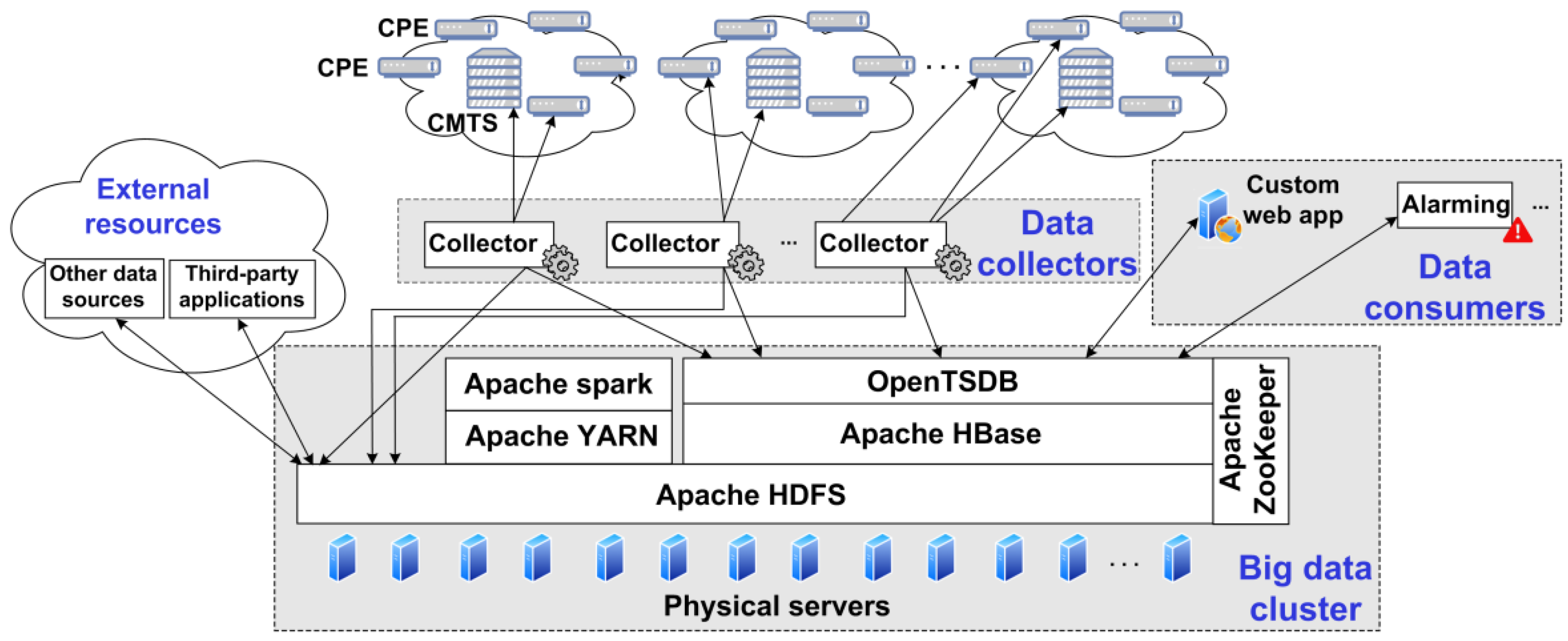
The logical architecture of BDPfPM is shown in Figure 2. The architecture comprises the following parts: monitored equipment, data collectors, big-data cluster, and data consumers.

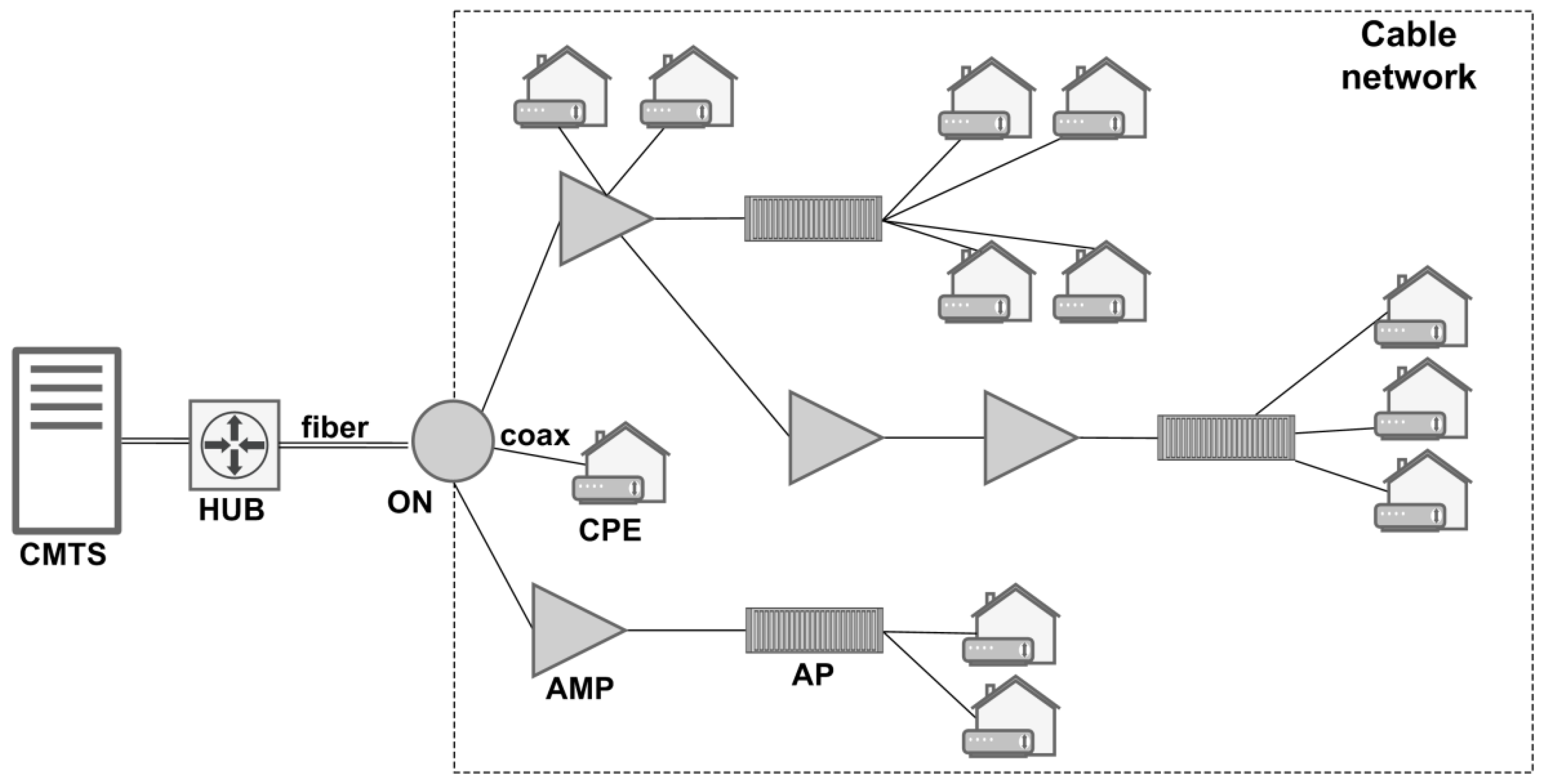
The monitored equipment are the devices in the HFC network capable of communicating with data collectors, such as CMTSs, cable modems, and set-top boxes. Cable modems and set-top boxes are CPE equipment on users’ premises. Performance metrics are collected from the network devices (CMTSs and CPEs) using SNMP. SNMP is chosen because all the intelligent devices (CMTSs, CPEs) in the HFC network support SNMP.

Table 1. Performance metrics.

Data Source	Performance Metric	CF [min]
CMTS	cpmCPUTotal5sec (overall CPU utilization in the last 5 s)	5
CMTS	ciscoMemoryPoolFree (free RAM memory)	5
CMTS	ciscoEnvMonTemperatureStatusValue (current temperature measurement)	5
CMTS	cdxCmtsCmTotal (total count of the CMs)	1
CMTS	cdxCmtsCmActive (total count of the active CMs)	1
CMTS	cdxIfUpChannelCmRegistered (total count of registered and online CMs on upstream)	1
CMTS	cdxCmtsCmRegistered (total count of registered and online CMs on MAC domain)	15
CMTS	docsIfSigQSignalNoise (signal-to-noise ratio for particular channel)	5
CMTS	ccsUpSpecMgmtCNR (carrier-to-noise ratio for particular channel)	5
CMTS	ifInErrors (total number of packets containing errors)	5
CMTS	ifHCInOctets (total number of upstream octets received on interface)	5
CMTS	ifHCOutOctets (total number of downstream octets sent on interface)	5
CMTS	docsIfUpChannelFrequency (center of frequency band associated with this upstream interface)	30
CMTS	docsIfCmtsCmStatusValue (CM status value)	60
CMTS	ccsFlapTotal (total number of flaps)	60
CMTS	docsIf3CmtsCmUsStatusSignalNoise (signal-to-noise ratio for upstream data from the CM on this upstream channel)	60
CMTS	docsIf3CmtsCmUsStatusRxPower (receiving power of this upstream channel)	60
CMTS	docsIfDownChannelPower (operational transmission power)	60
CMTS	docsIfCmStatusTxPower (operational transmission power for the attached upstream channel)	60
CMTS	docsIfSigQSignalNoise (average signal-to-noise ratio on upstream level)	60
CMTS	ifInOctets (total count of octets received from CM)	60
CMTS	ifOutOctets (total count of octets sent to CM)	60
CPE	docsIfDownChannelPower (received power level)	60
CPE	docsIfCmStatusTxPower (operational transmission power for the attached upstream channel)	60
CPE	docsIfSigQSignalNoise (signal-to-noise ratio of downstream channel)	60
CPE	ifInOctets (total count of received octets)	60
CPE	ifOutOctets (total count of sent octets)	60

shows a recommendation for the performance metrics collected from the CMTSs and CPEs that can be used for performance-monitoring purposes. All the metrics in Table 1 are used in BDPfPM. Other metrics can be added to the collector in case they are required. This table presents a more detailed representation of the performance metrics proposed in [23], with a given collection frequency (CF). The main difference between the list given in [23] and Table 1 is in the separate presentation of the metrics collected from CMTS, but related to the CPE equipment. The CMTS performance metrics in Table 1 are given for one Cisco CMTS model (uBR10000), while CPE performance metrics are given for Cisco’s CM model (EPC3928) because it is not possible to show all the performance metrics, given the variety of manufacturers and devices in the HFC network (Variety challenge). More details (like OID values) regarding performance metrics given in Table 1 can be found in [46]. Furthermore, Table 1 provides the performance-metrics collection frequency set for the real HFC network in which BDPfPM operates. Note that the CF values can be modified if necessary.

Data collectors are responsible for collecting data from the monitored equipment and transmitting the collected data to the big-data cluster. However, the importance of data collected from CMTSs and from CPEs differs. Furthermore, the responsiveness and availability of CMTSs are significantly higher compared to CPEs. Furthermore, not all performance metrics are equally important. Thus, the regular collection frequencies for CMTSs and CPEs differ. The same applies to the performance metrics. In BDPfPM, the collection frequency for CPEs, TCPE, is set to 1 h, while for CMTSs collection frequency, TCMTS, is set in the range from 1 to 60 min, depending on the collected performance metric. Note that the parameters TCPE and TCMTS can be set differently if required. Furthermore, the collection period for devices that are troubleshot is set to seconds during the troubleshooting process.

The data-collection layer has a manager that assigns to each collector a list of devices from which data, i.e., performance metrics, are collected. The assignment algorithm is simple. The manager uses a data-collector configuration to access a list of the CMTSs and CPEs connected to them. The data-collector configuration is a result of the MAC-IP-mapping mechanism described in Section 5.6. The manager passes a list of CMTSs in round-robin fashion. The round-robin method was selected because it is simple to implement. Given that the round-robin method achieved satisfying performances in our case, other methods were not considered. When data from CPEs served by currently passed CMTS in the list need to be collected, the manager sends a list of CPEs to a randomly chosen collector from the list of free collectors. The list of the CPEs passed to the collector also contains the IP addresses of the CPEs. These IP addresses are necessary because SNMP is used for data collection. One collector (four cores, eight GB RAM) can support collection from up to 25,000 CPEs for a TCPE value set to 1 h. In a similar fashion, CMTSs are assigned to collectors. CMTSs are assigned with a collection frequency set to a minimum TCMTS value, and the manager passes a list of performance metrics that need to be collected in that collection period. For example, according to the CF values in Table 1, cdxCmtsCmTotal would be collected in every collection period, while ifInErrors would be collected in every fifth collection period.

The collected data are enriched with appropriate tags, as explained in Section 5.4. Once the data are collected and enriched, they are sent directly to OpenTSDB using a web socket. Furthermore, a copy of the same data is saved to a file and written to the HDFS for data-aggregation purposes.

The big-data cluster performs storage and processing functions. The big-data cluster can additionally use data from external data sources and third-party applications. The total capacity of the cluster depends on the number of monitored devices, collection frequency, and defined retention policy. Since there is no official standard, the data-retention policy depends on operator preferences. Since the collected data are not related to the personal data, there is no regulation that enforces the data-retention policy. Our practice has shown that the data-retention period should be in the range of 3–6 months, depending on operator preferences and storage capacities. This retention period is sufficient for network troubleshooting and performance management. In BDPfPM, the data-retention period is set to 6 months. The information obtained from the processing of collected data is used by data consumers. Data consumers can be, for example, alarm systems, network operation center dashboards, call-center reporting software, etc.

Figure 2 shows that the big-data cluster comprises several big-data tools: OpenTSDB (Open Time-Series Database), Apache HBase, HDFS (Hadoop Distributed File System), Apache Spark, Hadoop YARN (Yet Another Resource Negotiator), and ZooKeeper. Collectors send messages that carry collected data to OpenTSDB. OpenTSDB accepts the incoming messages, reads them and verifies their format, and stores them in appropriate HBase tables. HBase stores table files to the HDFS, which stores the data on physical discs. Spark performs data aggregations. YARN allocates resources to jobs and enables different processing frameworks to use common hardware. YARN is used as a resource manager for batch jobs in the BDPfPM. Zookeeper provides synchronization between distributed services. The proposed big-data cluster satisfies all the initial requirements in terms of BDPfPM robustness, scalability, high availability, fault tolerance, and performance. The big-data cluster represents the central point of the overall architecture shown in Figure 2.

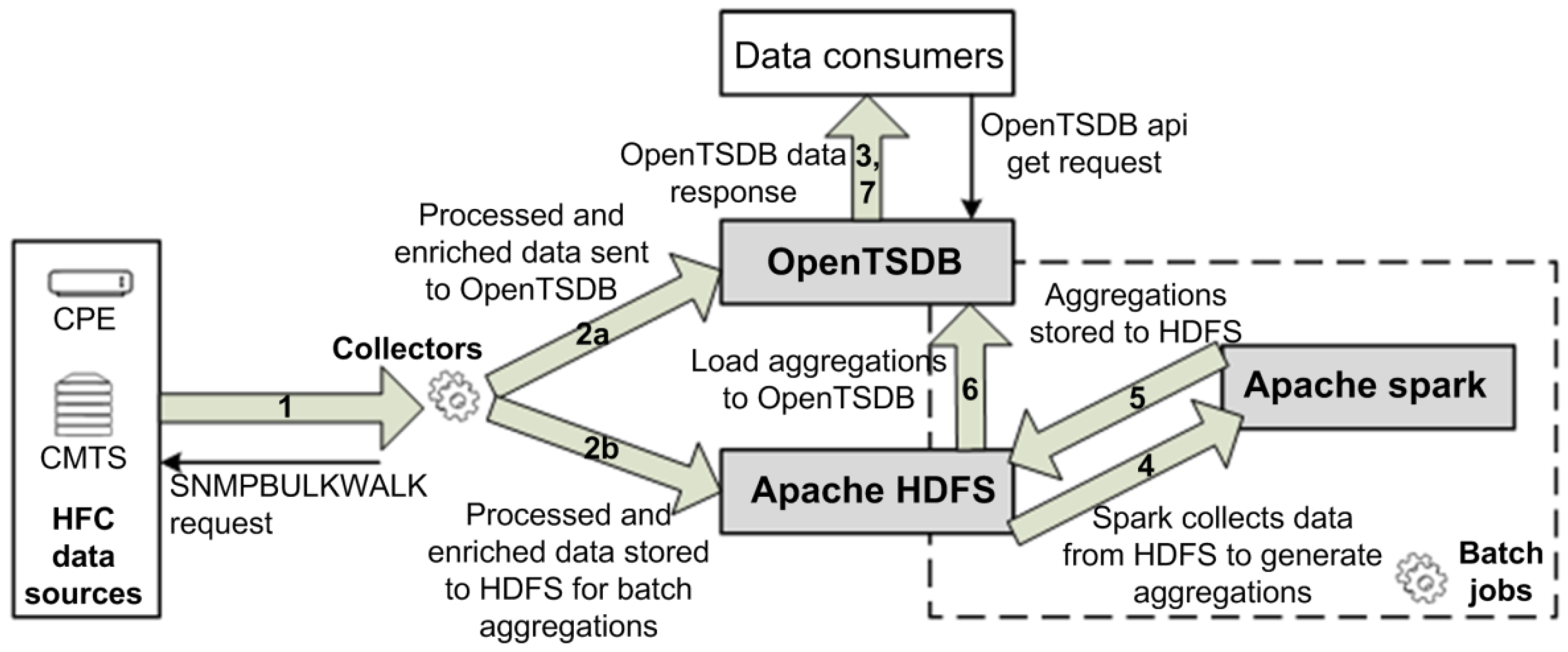
Figure 3 summarizes the previously described data collection and processing in the form of a collected-data flow from data sources in the HFC network to BDPfPM and data consumers. The collector sends the requests to the monitored devices and receives the data from data sources (1). The processed and enriched data are sent to the OpenTSDB using web sockets (2a). In parallel, the collector stores the copy of the data to the file and uploads it to the HDFS (2b). The data in OpenTSDB are ready for consumption immediately upon arrival (3). The data saved to the HDFS are further processed in batch jobs using the Apache Spark framework (4). The aggregations are stored back on theHDFS (5) and uploaded to OpenTSDB (6) for consumption (7).

The collected data are used for the performance monitoring of the HFC network. The main purpose of the collected data is the detection of weak spots in the network that need to be repaired to increase the overall HFC network performance and user QoE (quality of experience). This is explained in detail in a separate section (Section 6) as the main application of the collected data in BDPfPM.

As discussed at the end of Section 5.1, there are several ways to implement BDPfPM. BDPfPM is implemented and tested using on-premises hardware and Cloudera 5.14 distribution. The on-premises hardware approach was selected because the telecom service provider for which the BDPfPM was originally developed requested it. The implementation is performed on the 2-namenode/6-datanode cluster and each server comprises 32-core Intel Xeon CPUE5-2630 with 2.4GHz and 64GB RAM. This setup is deployed in a real HFC network. During the initial phase of deployment, the BDPfPM parameters (such as collection frequencies, number of retries, timeout values, and other parameters, discussed in later subsections) were tuned to optimize the BDPfPM performance. Thus, all the parameter values proposed in the following sections and subsections are based on the results of the experiments conducted in the real HFC network environment.

5.3. Data Schema

BDPfPM uses OpenTSDB to store the performance metrics collected from the HFC network. According to [41], OpenTSDB provides several ways to analyze and manipulate the collected data. In this subsection, we discuss the data-schema possibilities, and we propose a data schema that improves the query performance.

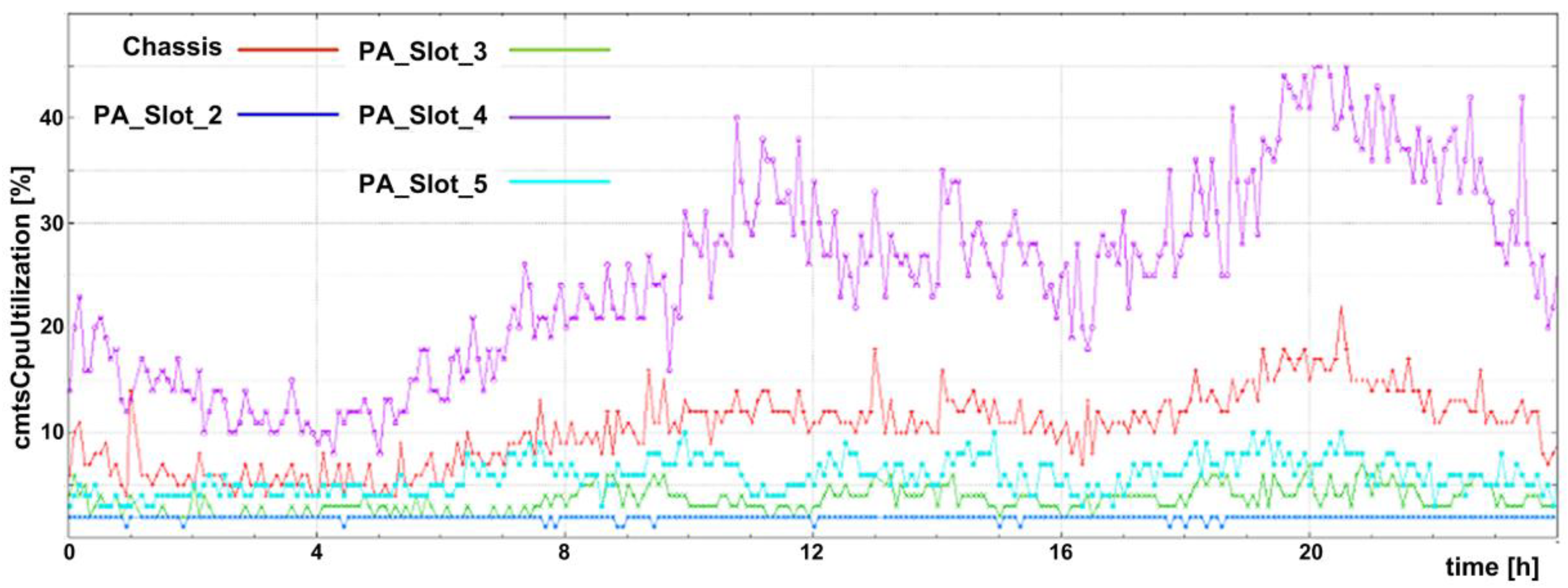
By using tags, it is possible to separate data points from different data sources. In this way, the data collected for one particular metric and a different set of tags can be easily observed, either separately or in groups [41], by using filtering or grouping. For example, Figure 4 shows the CMTS CPU (central processing unit) utilization per unit (tag “entity_name”) for one day. The graph in Figure 4 was generated using raw data collected from a CMTS device, named TEST-CMTS, that comprises five CPU units (their “entity_name” values are used in the legend of Figure 4). Note that the values of the tag, “entity_name”, are given in

Table 2. Average CMTS CPU utilization (cmtsCpuUtilisation).

Time	CPU Use	Entity_Name	Device_Name Cmts_Name	Device_Type	Cmts_Type	Entity_Type	Device_Ip	Company
1584658859	6	Chassis	TEST-CMTS	CMTS	Cisco	CPU	192.168.0.1	company1
1584658859	4	PA_Slot_3	TEST-CMTS	CMTS	Cisco	CPU	192.168.0.1	company1
1584658859	2	PA_Slot_2	TEST-CMTS	CMTS	Cisco	CPU	192.168.0.1	company1
1584658859	14	PA_Slot_4	TEST-CMTS	CMTS	Cisco	CPU	192.168.0.1	company1
1584658859	3	PA_Slot_5	TEST-CMTS	CMTS	Cisco	CPU	192.168.0.1	company1
1584658859	68	PA_Slot_1	TEST-CMTS2	CMTS	Cisco	CPU	192.168.0.2	company1
1584658859	42	PA_Slot_2	TEST-CMTS2	CMTS	Cisco	CPU	192.168.0.2	company1

. Since filtering was not used, the CPU utilization for all five units is shown in the graph. Using filtering by tag, it is possible to observe data only for a particular unit instead of the whole set. For example, if the filter were set to entity_name=Chassis, the graph in Figure 4 would show CPU utilization only for the Chassis unit. On the other hand, grouping merges multiple individual time series into one [41]. 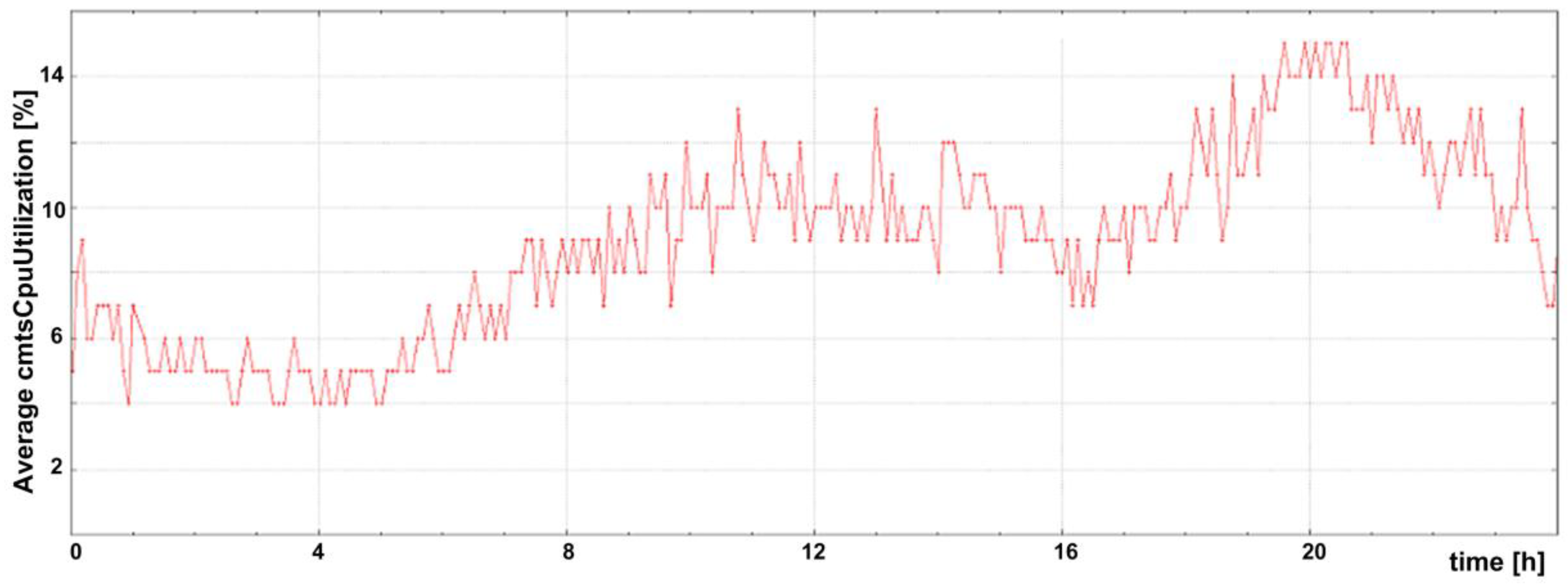An example of grouping is shown in Figure 5. Figure 5 shows the average CPU utilization for the same dataset as shown in Figure 4. The average CPU utilization is generated automatically from the raw data by omitting the tag, “entity_name”, from the query and setting “avg” as the aggregation type. The OpenTSDB web–user interface was used to generate the graphs in Figure 4 and Figure 5. In addition to the basic data aggregation types, OpenTSDB supports downsampling, as well as some advanced data aggregation types that are not within the scope of this paper.

Table 2 contains the data points for one KPI (cmtsCpuUtilisation) from two different data sources (TEST-CMTS and TEST-CMTS2) collected in one period of time (1584658859). When a user creates a query to collect the data for a particular metric, OpenTSDB performs data filtering based on given tags and time range. The query execution, i.e., data filtering time is directly proportional to the number of data points collected for one metric in one iteration. In HFC networks, there are millions of CPEs, each with several interfaces for data collection. Thus, data filtering for one device and its entities can be extremely slow, resulting in poor query performance.

To overcome this challenge, we propose a new data schema, in which the tag for the name of the monitored device (for example, the MAC address for the CPE, the hostname for the CMTS) is changed to the metric name (for example, cmtsCpuUtilisation is now named as cmtsCpuUtilisation_TEST-CMTS). In this way, a new metric is created for each device. This is a reasonable decision because queries relate to a particular device in most cases (for example, in call-center reports or troubleshooting reports for one particular modem). In this way, we increase the query performance by around 1300 times, according to our test scenario. In our test scenario, there are one million devices with four interfaces. The initial query time for extracting the data for one device from a group of one million devices was 307.041 s, while obtaining the same data from the proposed new data schema took 234 milliseconds. The testing was performed on the big-data-cluster setup described at the end of Section 5.2.

The downside of the proposed novel data schema is the impossibility of creating the group queries related to a particular device for other tags (for example, the queries grouped for all the modems per model type). However, it is not necessary to perform this kind of aggregation in a timely manner. Therefore, it is performed using Spark daily aggregation jobs. If the proposed data schema is used, one should be careful with the number of created metrics. According to [41], metrics are encoded with three bytes, giving 2^3×8 − 1 = 16,777,215 unique metrics. However, the number of bytes used for encoding the metric can be tuned via configuration, as in OpenTSDB version 2.2.

5.4. Data Collectors

The data-collection layer needs to be defined after the initial architecture for data storage is established. Data collectors are software components that collect data from sources, enrich data, and then format and send these data to the storage layer. The storage layer in BDPfPM comprises OpenTSDB for data consumption and HDFS as a stage for data aggregation, as shown in Figure 3. Some publicly available collectors can be used [41]. However, publicly available collectors usually cannot cover specific use cases, domains, and specific needs. Therefore, the custom development of data collectors is necessary.

Data collectors are created per integration domain. The integration domain is a logical unit for which monitoring is performed. For example, the integration domains can be DOCSIS, MPLS (multi-protocol label switching), UPS (uninterruptible power supply), QoS (quality of service), etc. Even these integration domains are further broken down into manufacturers, different models, and software versions. For example, Cisco CMTSs have different OIDs (Object Identifiers) and MIB (Management Information Base) tree structures from CASA or Motorola CMTSs; the Cisco CMTS Remote PHY platform differs from traditional Cisco HFC deployment [47].

The integration domain of interest for the BDPfPM is the DOCSIS domain for CMTS and CPE equipment. The DOCSIS domain covers the performance metrics defined in [23], such as the user, environment, and interface statistics for CMTSs, and the CPE statistics collected from CMTSs (metrics collected from CMTSs but concerning the CPEs) and directly from CPEs. Other domains, such as MPLS, WiFi, and others, will be a part of future work. Special attention is given to data-collector latency and efficiency because there are many monitored devices in the HFC network.

Client–server communication is used between the data collectors and data sources, in which the data collectors have a client role and the data sources have a server role. Since a custom data collector was developed, the integration with data sources can be established in a variety of ways, depending on its communication capabilities. REST API, JDBC (Java Database Connectivity), SNMP, HTTP (web crawling), subscriber–broker communication, file parsing (for example, log, or any other type of file that can be processed) are some of the possible approaches. The SNMP protocol is used for both CMTS and CPE equipment in BDPfPM. The SNMP was selected because all the CMTS and CPE devices currently installed in the HFC network support this protocol. However, other protocols and approaches will be added to BDPfPM in the future.

The SNMP protocol is configured with read-only permission on the monitored devices. The data collector uses appropriate community string and IP addresses to communicate with the monitored devices. Communication is established via SNMPGET and SNMPBULKWALK, depending on whether one or multiple responses are expected. SNMPBULKWALK is used instead of SNMPWALK because of its superior efficiency and faster query response.

In terms of timeout and number of retries, the SNMP configuration can significantly affect the data collector’s overall performance. In situations in which a monitored device is highly available, such as CMTS, the retry and timeout can be set to reasonable values, such as a timeout of two seconds and three retries (we propose these values based on the tests conducted in the real network). However, in the case of CPE monitoring, there is no guarantee that a monitored CPE device is available. Furthermore, the number of these devices in the HFC network is in the order of hundreds of thousands or millions. Thus, a significant increase in execution time occurs because data collectors spend a huge number of processing resources that are reserved a priori only for waiting for the responses from unavailable CPEs. The timeout and retry time should be carefully selected to minimize the impact of this phenomenon. After conducting tests in the real network, we suggest a one-second timeout and one retry for CPEs in order to provide optimal results. If the monitored device does not answer the query after 1 s, the device is most likely unavailable.

The collected data (performance metrics) are enriched with an appropriate set of tags. Measurement by itself has little value without tags. The tags are information-packed in key-value pairs that uniquely define the source of the measurement [41]. There are two types of tag: mandatory and optional. During data-collector development, it is necessary to find all the tags that describe the measurement, identify mandatory tags, and filter only those that are of interest. The mandatory tags are all the tags necessary to distinguish data by source. In the example shown in Table 2, the device_name and entity_name tags are mandatory because these tags separate CPU utilization per device and processor unit. If some of these tags were omitted, the collected measurements would have the same set of tags, causing the overlap of collected data, leading to inaccurate information.

Optional tags are used to further enrich the measurement. The greater the number of different tags, the greater the number of different aggregation types that can be performed. For example, the CPE vendor and model are not relevant when data are collected. However, these tags are used later for data aggregation and analysis, which provide insights into performance for each of the vendors and models. These insights are valuable sources of information when acquiring new equipment. One should not exaggerate the use of optional tags, but use only those that are used for data aggregation. If a tag is found to be important, it can be added later without disturbing the previous measurements. Aggregation per new tag is available from the moment of its addition.

There are four types of metrics in CMTS data collection:

• Environment;
• Upstream;
• Downstream;
• MAC domain.

Environment metrics provide information regarding the physical health of a device (such as processor utilization, free memory, and temperature), while upstream, downstream, and MAC domain metrics are related to KPIs (such as SNR—signal-to-noise-ratio, CNR—carrier-to-noise ratio, error rate, and throughput) collected on the levels they describe [23]. These metrics share common tags, such as device_name, device_type, device_vendor, and company_name. However, the tags regarding interfaces differ according to their groups. For example, upstream interfaces are connected to load balance groups, while downstream interfaces are not.

Data can be sent to OpenTSDB in a variety of ways; web socket and file import are the most common. Both of these approaches are used in BDPfPM. Web socket is used to send data from data collectors to OpenTSDB, while file import is used for importing Spark aggregation results into OpenTSDB.

Before data are sent through a web socket, the data collector needs to check whether OpenTSDB is available and establish a connection. The OpenTSDB availability check is performed because of the congestion problem that occurs due to the large amount of incoming traffic. To overcome this problem, we defined a list of OpenTSDBs and their appropriate communication ports. The data collector randomly selects one OpenTSDB from the list, checks its availability, and sends the data. If the selected OpenTSDB is unavailable, another option from the list is selected, and the procedure is repeated. The data collector tries to send the data until it uses up all the OpenTSDBs from the list. In this way, OpenTSDBs’ high availability and even load distribution are ensured.

Data can also be sent to OpenTSDB using file import. This is possible only in situations in which collectors and OpenTSDB share hardware. This method is rarely used in data collectors. However, this method can be extremely useful in situations in which Spark aggregation results are imported in OpenTSDB. This is possible since these two are installed on the same hardware, according to the proposed architecture. The results are imported directly from the file. Thus, the socket load is reduced and the availability is increased.

Due to the specific data schema that is used (metrics are further broken to metric_device-name as described in Section 5.3), the data stored in OpenTSDB are not suitable for batch aggregation. To overcome this challenge, the data collector, in addition to sending messages to OpenTSDB, stores a copy of the collected data in text files and uploads these files to HDFS. How long the data are stored on HDFS depends on the aggregation requirements. Note that this retention period additionally increases the storage capacity requirements. For example, to support weekly aggregations, the minimum required retention period for keeping the raw data on Apache HDFS is 7 days. A buffer for a couple of additional days is usually added in case there is a problem with the aggregation. Therefore, to support weekly aggregations, a 10-day retention period would be sufficient. In the case of other aggregations, such as daily or monthly, the retention periods would be defined in similar fashion.

5.5. Data Aggregations

Raw data collected directly from the network are useful for performance monitoring, troubleshooting, and other daily operations. The collected data can be aggregated to provide deeper insight into the state of the network. Using proper data aggregations, telecom service providers can obtain valuable information for decision making and business planning. This topic highlights all the possibilities of BDPfPM win terms of aggregations, but does not list all those that have been developed, as they exceed the scope of this paper. Each aggregation type is enforced by a concrete example.

There are several different types of data aggregation, depending on the desired goal. Aggregations can be split into time and spatial aggregations. Time aggregations are aggregations of data collected during a certain period (for example, daily, weekly, monthly) into one data point. Spatial aggregations are aggregations of different data sources in each period. Figure 5 from Section 5.3 represents an example of spatial aggregation. TEST-CMTS CPU utilization is aggregated into a single average value for every collection interval. In this way, the overall CPU utilization of the monitored device is obtained. This is a much better way of monitoring devices’ CPU utilization because the temporary peaks of individual cores are mitigated. Depending on the moment of execution, batch or stream aggregation are used. Batch aggregation is performed after the data are collected. On the other hand, stream aggregation catches the data at their source and performs aggregation in real time. In this paper, we focus on batch aggregation.

BDPfPM uses big-data aggregation tools due to the large amount of data that need to be processed. In comparison to traditional data-processing methods, big data performs distributed processing in a master–slave manner. This approach is scalable because it uses load distribution across multiple servers. We use Spark as a data-aggregation processing tool in BDPfPM (for batch aggregation).

There are two types of data aggregation in BDPfPM: OpenTSDB and batch aggregation. OpenTSDB can perform both time and spatial aggregations using its built-in functionalities. Spatial aggregations are performed based on tag grouping in the request query. Time aggregations are performed using the downsampling feature. Using these functionalities, OpenTSDB provides a simple interface to perform complex and effective aggregations from raw data. Thousands of data points are aggregated in the order of milliseconds. OpenTSDB is especially useful when aggregation for one particular device is required (CMTS or CPE in HFC network).

Batch aggregations are used to provide deeper insights based on the collection of large data sets. Batch aggregations are slow because of the enormous amount of data that is processed and are therefore not time-sensitive. Apache Spark is used for batch aggregations in BDPfPM. In practice, batch aggregations are useful in many different applications. In HFC networks, these aggregations are used to provide better insights into the network performance on a variety of levels. These levels are defined per application. One example of a hierarchy that is typically used is: upstream, MAC domain, CMTS, city, territorial direction, state, and company, respectively. The levels up to CMTS are used to observe the statistics for a particular device, while higher levels are used for company analysis. Most batch aggregations are performed using the data collected from CPEs because they give insights into the state of the network from the end-user’s perspective.

One example is network availability based on CPE data, which gives telecom service providers information about the network availability on different hierarchy levels from the end-user’s point of view. This metric is created based on CPE availability time; the availability of every CPE is calculated on a daily basis. The end-user’s point of view is important because measuring network unavailability from this perspective gives a direct insight into users’ quality of experience. Another example of batch processing is performance monitoring for network devices that cannot provide statistics about their health (non-intelligent devices). The raw data collected from CPEs are combined with the network topology to obtain information regarding the health of devices that cannot be monitored directly, such as APs, AMPs, and ONs.

Data aggregations can be used beyond the performance-monitoring application in our proposed BDPfPM. For example, the raw data collected from CPEs can be combined with user-service-agreement information. The first potential application of such data aggregation is to isolate all the clients that have premium packets, but poor quality of service. The second potential application is to isolate heavy users with small subscription packets to offer them larger subscription packets. These simple examples show the promising potential of BDPfPM for applications beyond performance monitoring.

5.6. Performance Comparison

In this subsection, we compare the proposed BDPfPM to other solutions. However, the solutions used by telecom service providers are usually not presented in the available literature. In this paper, we compare BDPfPM to the big-data framework for performance management in mobile networks (BDFMN) presented in [36], since it is the most similar solution to BDPfPM in the literature.

BDFMN is not actually implemented in the real network, but it uses data sets from the real network. Based on these data sets, data-set replicas are generated for testing purposes. BDFMN is simulated for a mobile network of 15 million subscribers in [36]. Base stations are data sources in the case of BDFMN. Other network elements (e.g., core network elements) are not considered in BDFMN. Thus, monitoring in BDFMN does not cover all the devices in the network. BDPfPM monitors the complete network and all its elements, including non-intelligent network elements, as discussed in the following section. Base stations for different mobile network generations (2G, 3G, 4G, 5G) were thought to coexist in the experiment, and the number of base stations simulated in the experiment was 13,300. Thus, the number of data sources in BDPfPM is significantly larger than in BDFMN, because BDPfPM collects data from devices associated with subscribers, i.e., CPE devices. Regarding availability and responsiveness, CMTSs and base stations are similar. However, in BDPfPM, there are CPE devices from which data are also collected. Subscribers can power off their CPE devices whenever they wish. This represents an additional challenge for the data-collection layer because data-collector resources can be wasted in trying to collect data from unavailable devices. BDPfPM successfully addresses these challenges, and there is no certainty that BDFMN would successfully address these challenges, since it was not tested for such cases.

BDFMN uses a collection period of 15 min. Regarding BDPfPM, the collection period is similar for metrics collected from CMTSs—for most of these metrics, the collection period is set to 5 min. CPE metrics are typically collected on an hourly basis, except in troubleshooting cases, in which the data collection period is set in the order of seconds. BDFMN collects XML files from the base stations and, for this reason, Flume is used for data collection, along with the SFTP (SSH File Transfer Protocol). On the other hand, BDPfPM uses custom-made data collectors that use the SNMP to collect performance metrics. Thus, differences regarding data collectors are a consequence of different network-element capabilities and data presentations. An additional difference is that BDPfPM enriches the collected data with appropriate tags, which gives extra flexibility and a higher level of granularity during data aggregations, as explained in Section 5.3. To store data, both BDPfPM and BDFMN use HDFS. The storage requirements in BDFMN are around 26 GB on a daily basis [36]. In the case of BDPfPM, for a network comprising around one million subscribers (the real HFC network in which BDPfPM is deployed), the storage requirements are around 320 GB. Obviously, the Volume challenge is greater in the case of BDPfPM, which is a consequence of the performance-monitoring coverage of all the network devices, including a great number of CPEs. For batch processing, BDPfPM uses Spark, while BDFMN uses Hive.

An important aspect is deployment. BDPfPM operates in the real network, while BDFMN uses the proposed framework, which uses data sets from the real network (along with data-set replicas). This makes an important difference, because actual deployments usually carry some unpredictable problems and challenges, as we discuss in Section 7 (BDPfPM deployment experiences). Furthermore, BDPfPM is used to estimate the health of devices that are not capable of performing measurements (non-intelligent devices), as explained in the following section. This is a challenge that is not analyzed in BDFMN.

Table 3. BDPfPM and BDFMN comparison.

Feature	BDPfPM	BDFMN
Number of data sources	Millions	Tens of thousands
Collection period	1–60 min	15 min
Daily storage requirements	320 GB	26 GB
Data collectors	Custom made, SMTP	Flume, SFTP
Data-storage technology	HDFS	HDFS
Batch-processing tool	Spark	Hive
Network-device coverage	Complete	Partial
Deployed in the real network	Yes	Partially

summarizes the comparison between BDPfPM and BDFMN. BDFMN is noted as being partially deployed in the real network because it uses data sets from the real network.

6. Performance Estimation of Network Devices

The data collected from monitored devices are used to grade their QoO (quality of operation). However, there are also non-intelligent devices in the HFC network that affect the quality of the network, but whose performance cannot be collected directly (ONs, AMPs, and APs). Therefore, the data collected from CPEs are combined with network-topology information to perform QoO estimations for these devices. The estimation results are written to the OpenTSDB and available for consumption as any other KPI. Using a custom web application, telecom service providers can perform various data aggregations to check the HFC network performance. One example used in BDPfPM is the estimation of the QoO of monitored devices. The QoO of a device can be estimated and graded from the collected data for a given period (daily, weekly, or monthly) to check its overall performance. Such information is used for predictive maintenance. In cases in which a device has low grade for long periods of time, the device is a weak spot that should be replaced or repaired. In this section, we describe in detail the method used for grading the performances of CPE devices, and the usage of these grades to estimate the performance of the non-intelligent devices.

The performance metrics used for grading the performance of CPE device are:

• cpe.docsIfDownChannelPower—collected from CPE;
• cpe.docsIfSigQSignalNoise—collected from CPE;
• cpe_cmts.docsIf3CmtsCmUsStatusRxPower—collected from CMTS;
• cpe_cmts.docsIfSigQSignalNoise—collected from CMTS

The explanations of these metrics are given in Table 1, in Section 5. These selected performance metrics provide information about the signal power in the transmitting and receiving directions. The first step in the estimation of CPE performance is the individual grading of each collected performance-metrics sample. Sample grading enables the same grade scale for all metrics and all samples. In this way, further processes of performance estimation based on the combination of selected metrics areenabled. The grade scale comprises three possible values: 1—poor, 2—medium, and 3—good.

Table 4. Mapping of performance metrics onto the unified grade scale.

Performance Metrics	1—Poor	2—Medium	3—Good
cpe.docsIfDownChannelPower	X ≤ −10 or X ≥ 17	others	−6 ≤ X ≤ 10
cpe.docsIfSigQSignalNoise	X ≤ 28	others	X ≥ 33
cpe_cmts. docsIf3CmtsCmUsStatusRxPower	X ≤ −21 or X ≥ 21	others	−11 ≤ X ≤ 11
cpe_cmts.docsIfSigQSignalNoise	X ≤ 21	others	X ≥ 28

shows the mapping of the four selected performance metrics onto the grade scale used.

Note that the values shown in Table 4 can be modified and adjusted to the specific needs and requirements of telecom service providers. The same applies to the grading scale, which can be redefined to be more granular. However, the conducted tests in the real network have shown that the grade scale defined in this section achieves satisfying results. Figure 6 shows the grade results for one CPE, which is connected to three downstream and two upstream channels. Grade 1 is represented by a red, grade 2 by a yellow, and grade 3 by a green circle.

Since the CPE can be connected to multiple upstream and downstream channels, multiple grades can be sampled for each performance metric in the same collection period—one for each channel (upstream or downstream, depending on the metric). However, it is preferable to have only one grade for each performance metric because this simplifies the combination of all the selected performance metrics. Thus, the multiple grades for the same performance metric are merged into one grade by using the worst-case method, in which the worst grade is selected. Figure 7 shows the results of the merge method for the example shown in Figure 6.

The next step is to combine these merged grades of all the performance metrics to obtain the final performance grade of the CPE. However, different performance metrics collected at the same collection period do not have the same timestamps, i.e., they are not collected at exactly the same moment. This can be seen in Figure 7, where there is an observable offset between the grades of different metrics in time domain. For this reason, the actual collection times are modified to the corresponding collection period start. In this way, all four performance metrics are aligned in time.

After the alignment, the merged grades that correspond to the same collection period are combined for all the collection periods that fall into the observation period for which the performance is estimated. The observation periods can be, for example, daily, weekly, monthly, etc. The combination of the performance grades of different metrics for one collection period is performed in the following way:

$$G_i=\frac{{\displaystyle {\sum }_j{W}_{j}P{G}_j}}{{\displaystyle {\sum }_j{W}_j}}$$

where G_i is the combined performance grade for the collection period i, PG_j is the grade of the performance metrics j for collection period i, and W_j is the weight factor of the performance metrics j. The obtained results for grade G_i are then adjusted to the grade scale by using the definitions given in

Table 5. Thresholds for combined grade G_i.

Gi	Thresholds
1	X < 2
2	others
3	X ≥ 2.75

.

Finally, the last step is to use grades G_i to determine the final performance grade FG of the CPE for the observation period.

Table 6. Thresholds for the final performance grade FG.

FG	Thresholds
1	more than 20% samples have grade 1
2	others
3	more than 85% samples have grade 3

defines how the FG is determined. The values defined in Table 5 and Table 6 were obtained based on tests in the real HFC network. Note that the values in Table 5 and Table 6 can be modified and adjusted to specific telecom-service-provider needs. Figure 8 shows the final performance grade FG for the example shown in Figure 6. Note that the performance-metrics collection times are aligned in Figure 8. Furthermore, all the weight factors W_j are set to equal value in the given example.

Based on the CPE performance grades, it is possible to estimate the performances of non-intelligent devices. The requirement is to obtain network-topology knowledge that provides information for each non-intelligent device about the CPEs that are hierarchically below the corresponding non-intelligent device. If this requirement is fulfilled, then the performance grades of the corresponding CPEs are used to estimate NFG—the performance grade of a non-intelligent device—according to the rules given in

Table 7. Thresholds for the performance grade of non-intelligent devices.

NFG	Thresholds
1	more than 50% of CPEs have FG = 1
2	others
3	more than 70% of CPEs have FG = 3

. Again, we emphasize that the values given in Table 7 were obtained via test conducted in the real HFC network, and that these values can be modified and adjusted according to the specific needs of the telecom service provider. Practice has shown that, over time, the average grade of all the devices in the HFC network increases because weak spots are detected and replaced or repaired in a timely manner.

7. Deployment Experience

During the development of BDPfPM, the main goal was to establish a highly available, scalable, and cost-effective platform capable of storing a huge amount of data, satisfying query-performance requirements, and performing advanced data aggregations. The big-data architecture proposed in Section 5 satisfies this main goal. However, new challenges emerged during the BDPfPM deployment. In this section, we present our experience during the BDPfPM deployment.

One set of challenges during the BDPfPM deployment relates to the OpenTSDB component configuration and implementation. The first problem was OpenTSDB traffic congestion. The congestion was a consequence of the huge amount of incoming data that the OpenTSDB component needed to parse and store into HBase. Furthermore, the query requests waited in a queue for OpenTSDB to parse them. Our first approach was to increase the OpenTSDB memory size by setting appropriate Xms and Xmx JAVA parameters. This approach improved the performance, but did not completely solve the congestion problem.

The second approach was to add multiple OpenTSDB instances. This approach solved the congestion problem. In this approach, all instances share common tables in HBase. HBase manages the access, thus maintaining the consistency of the tables. Each data collector sends data to a randomly selected OpenTSDB instance from the list of existing instances. In this way, incoming traffic is evenly distributed among the OpenTSDB instances. Furthermore, some OpenTSDB instances are set only to read query requests to maximize query response time. To minimize the traffic latency between HBase and OpenTSDB, OpenTSDB instances are installed on existing big-data servers, i.e., on namenodes and datanodes. This second approach solved the OpenTSDB traffic-congestion problem and even introduced scalability to the OpenTSDB component of the big-data cluster.

The second OpenTSDB-related problem was associated with the metric UID (unique identifier). OpenTSDB creates UIDs to save metrics. The number of bytes used for the metric UID value is called the UID size parameter. The UID size is three bytes, as mentioned in Section 5. Using the data schema proposed in Section 5.3, this pool of possible UID values can be quickly spent. One approach to solving this problem is to increase the UID size (available from OpenTSDB version 2.2). For example, if the UID size is four bytes, it is possible to have 2³² − 1 different values of UIDs. The optimal UID size value is estimated based on the number of monitored devices and the number of metrics. However, it is still possible to spend all the UID values due to the increasing number of devices or integration with new domains. This limits the BDPfPM scalability and integration to new domains. Once the UID size parameter is set, it cannot be easily changed in the future. Therefore, if there were a need to increase UID size value, HBase tables would be recreated with a new UID size value, which would cause a loss of historic data. Thus, we propose the second approach, which prevents the aforementioned problem.

In the proposed approach, we use a separate set of tables per integration domain with an appropriate set of OpenTSDB instances instead of using one set of HBase tables. This approach should be applied not only in the integration to new domains, but also in multitenancy cases, as well as any other cases in which data do not need to stay together. The proposed approach has several benefits:

• In general, the main data table is split, which additionally increases the query performance.
• For every set of tables, an appropriate UID size can be set, providing a better estimation of incoming traffic.
• It offers a better multitenancy approach. Each country has its own set of tables. If the data for some countries need to be deleted, this is easily performed by dropping the appropriate set of tables. Otherwise, it is very difficult and time-consuming, because data need to be deleted per metric and per device.
• It offers a flexible data-retention period. The retention period is set on the HBase level by configuring table properties (time to live parameter). Using the proposed approach, each set of tables can have a different retention period.

The next challenge during the BDPfPM deployment was associated with the problem of needing IP addresses to identify the CPEs in the HFC network. As we mentioned in Section 5.2, IP addresses are required because the SNMP is used for data collection. Thus, the IP address of the CPE is needed to establish SNMP communication between the data collector and the CPE. The CPE device in the HFC network has a dynamic IP address. When a CPE connects to a network, it receives a local IP address from a predefined pool. This approach is common in HFC networks. The first problem is to monitor CPEs, because they can change their IP addresses overtime. Consequently, the IP address cannot be selected as the unique identifier for CPE. Instead, the MAC address is used as a primary key. However, BDPfPM needs IP addresses to communicate with CPEs to collect data. Thus, it is necessary to establish mapping between the MAC and IP addresses of CPEs. We propose a MAC-IP-mapping mechanism, which is described in the following paragraph.

Information about the mapping between CPE’s MAC and IP address is periodically collected from the corresponding CMTS. The collected information is used to create a data-collector configuration. This configuration is later used to establish a connection with the monitored CPEs for data collection. The MAC-IP-mapping mechanism runs a few times a day, usually three. This approach has one downside. CPEs that change IP address between the MAC-IP-mapping updates is unavailable for data collection until the next update. Fortunately, the practice shows that the address for one CPE rarely changes. Changes may occur after CPE restart. Even then, in the majority of cases, the CPE receives the same IP address. However, we eliminate this downside by minimizing the MAC-IP-mapping mechanism execution period to one data-collection period. This is justified because the greater number of generated CMTS queries is negligibly small compared to the total number of queries generated by the data-collector side. Thus, minimizing the MAC-IP-mapping mechanism’s execution period does not significantly affect the CMTS performance.

The next set of challenges during the BDPfPM deployment was associated with the data-collection process. There are multiple instances of data collectors due to the large number of monitored devices. Each collector collects data from as many devices as it can in a defined time frame (with some extra capacity left). The collector processes one device at a time until it has processed all the assigned devices. When the monitored device is offline, or communication with the collector is slowed down, the processing time is greater than usual. In situations in which group failure occurs (e.g., power failure, network failure), a group of devices becomes unavailable. This significantly increases the collector’s processing time. Thus, the collector cannot collect data in a defined time frame from the available devices.

We propose parallel processing instead of serial processing to overcome this problem. Each device is processed in a separate thread. If adevice is unavailable, this affects only the thread that it uses. Furthermore, this approach speeds up the collection process by multiple times. The approach requires collectors with more processing power, but fewer processing machines. In addition to solving the problem of unavailable devices, this approach reduces the total CPU and memory resources needed for the collectors. However, the number of parallel processes on data collectors should be carefully selected. After the conducting tests in the real network, we suggest that 30–50 devices per processing core should be set to run in parallel to achieve excellent results. If the selected number is too large, collector congestion may occur. Note that the optimal number of parallel processes directly depends on the collector architecture. For this reason, we recommend tests after a new data collector is developed to determine the optimal number of parallel processes.

The data collected from CPEs are essential during troubleshooting and performance monitoring. Every CPE is connected to the CMTS and the appropriate set of upstreams. Unfortunately, monitored CPEs do not know to which CMTS and upstreams it is connected. Thus, it would be beneficial to enrich the data collected from the CPE with information from the CMTS. We propose an add-upstream-info mechanism to enrich the data collected from the CPE with information from the CMTS. The add-upstream-info mechanism performs data collection from the CMTS. A combination of CPE MAC addresses and upstream frequency is taken as a key for one CPE and its upstream. This key is later used at the CPE-collector level to obtain the lookup data. The enriched data are stored in a lookup file and forwarded to the collector. The data collector collects the upstream frequencies from the CPE. Based on these data and the MAC address, the collector finds tags from the CMTS. When the add-upstream-info mechanism was deployed, slow file reading was encountered. On average, one collector (four cores, eight GB RAM) collects data from 25,000 devices. This means that the lookup file can have up to 100,000 lines. Intuitively, this file is large and slow to read. To overcome this problem, we propose the following method. Instead of creating one big file, several smaller files are created. Now, one lookup file only contains information for one modem and its upstreams. This significantly reduces the collector’s processing time. Furthermore, when one device is processed, its lookup data are discarded; thus, the occupied amount of the collector’s memory is reduced.

8. Concluding Remarks and Future Work

Telecom service providers can collect a large amount of data. Thus, the application of big-data technologies is very attractive to telecom service providers as it can allow them to extract and obtain valuable information from collected data. The obtained information can be used to improve the network performance. In this paper, we propose BDPfPM. The proposed BDPfPM is successfully deployed and used in practice. The average grade of network devices has been steadily increasing over time because poor-performance devices have been detected and replaced in a timely manner. Consequently, this has reduced the number of failures in the network and the number of complaints from subscribers. The responses to questionnaires showed the increased satisfaction of subscribers because of the better and more reliable network performance. The solutions and experiences presented in this paper can help others to building their own performance-monitoring solutions. However, we will continue to work on BDPfPM to further improve its performance and to extend it with additional features that reach beyond the performance-monitoring scope. In the remainder of this section, we discuss the limitations of BDPfPM and our future work regarding them.

There is an ongoing tendency to eliminate the time between the creation and consumption of data. Regarding this tendency, BDPfPM needs to support both real-time (streaming) and batch processing. Popular architectures for streaming data processing that are currently in use are lambda and kappa [48]. The most important limitation of BDPfPM is its lack of support for streaming-data processing. For the initial purpose of network-performance monitoring, BDPfPM does not require significant streaming-data processing support. However, adding this support would raise BDPfPM’s portfolio to an even higher level and enable the potential use of BDPfPM in domains and industries that have a significant need for streaming-data processing. Thus, our future work will focus on expanding BDPfPM to efficiently support streaming-data processing. For this reason, we will consider software components such as Kafka, Flink, etc. The second limitation is the partially addressed Veracity challenge. The important part of the Veracity challenge that is solved is the fact that BDPfPM enables the collection, storage, and processing of complete data sets instead of partial data subsets. Out-of-bounds metric values are detected and marked as invalid; thus, these values are not taken into account during data aggregations. Furthermore, if, in multiple collection periods, out-of-bounds values are collected from the same device, an alarm notification is sent to the alarm system to notify the operator about the suspicious behavior of the device (e.g., there might be a mismatch between the firmware version expected by the data collector and actual version loaded in device). A further work in progress is the automatization of the detection of the reason for absent performance-metric values—these might include power outage, link failure, users powering-off the CPE device, and device malfunction. BDPfPM is used for the collection, storage, and aggregation of performance metrics from the HFC network. However, BDPfPM can be used in other domains and industries. In our future work, we intend to expand BDPfPM to support domains such as MPLS, WiFi, etc. Furthermore, the IoT and sensor networks aresources of time-series data that can be collected, stored, and processed by BDPfPM. In our future work, BDPfPM will be expanded to support these data sources. The BDPfPM expansion for other domains (MPLS, WiFi, IoT, etc.) is possible due to BDPfPM’s flexible and scalable architecture. The main adjustments need to be made in the data collection layer by adding the data collectors designed to collect data from new devices that exist in the added domain. Furthermore, depending on the type of information these data contain, a new set of aggregations should be written to extract the information for the consumers of data in this domain. However, these adjustments do not affect the overall BDPfPM architecture, which remains the same.

References

1. Chen, M.; Mao, S.; Liu, Y. Big data: A Survey. Mob. Netw. Appl. 2014, 19, 171–209. [Google Scholar] [CrossRef]
2. Emani, C.K.; Cullot, N.; Nicolle, C. Understandable Big data: A Survey. Comput. Sci. Rev. 2015, 17, 70–81. [Google Scholar] [CrossRef]
3. Benhavan, T.; Songwatana, K. HFC network performance monitoring system using DOCSIS cable modem operation data in a 3 dimensional analysis. In Proceedings of the JICTEE 2014, Chiang Rai, Thailand, 5–8 March 2014; pp. 1–5. [Google Scholar] [CrossRef]
4. Park, J.; Lee, M. QoS Provisioning Method for Downstream VoIP Service Flows in HFC Networks. IEEE Trans. Consum. Electron. 2007, 53, 448–453. [Google Scholar] [CrossRef]
5. Ghorbanian, M.; Dolatabadi, S.H.; Siano, P. Big Data Issues in Smart Grids: A Survey. IEEE Syst. J. 2019, 13, 4158–4168. [Google Scholar] [CrossRef]
6. Chen, M.; Yang, J.; Hu, L.; Hossain, M.S.; Muhammad, G. Urban Healthcare Big Data System Based on Crowdsourced and Cloud-Based Air Quality Indicators. IEEE Commun. Mag. 2018, 56, 14–20. [Google Scholar] [CrossRef] [Green Version]
7. Wang, T.; Liang, Y.; Zhang, Y.; Zheng, X.; Arif, M.; Wang, J.; Jin, Q. An Intelligent Dynamic Offloading from Cloud to Edge for Smart IoT Systems with Big Data. IEEE Trans. Netw. Sci. Eng. 2020, 7, 2598–2607. [Google Scholar] [CrossRef]
8. Siddiqa, A.; Karim, A.; Gani, A. Big data storage technologies: A survey. Front. Inf. Technol. Electron. Eng. 2017, 18, 1040–1070. [Google Scholar] [CrossRef] [Green Version]
9. Boubiche, S.; Boubiche, D.E.; Bilami, A.; Toral-Cruz, H. Big Data Challenges and Data Aggregation Strategies in Wireless Sensor Networks. IEEE Access 2018, 6, 20558–20571. [Google Scholar] [CrossRef]
10. Flouris, I.; Giatrakos, N.; Deligiannakis, A.; Garofalakis, M.; Kamp, M.; Mock, M. Issues in Complex Event Processing: Status and Prospects in the Big Data Era. J. Syst. Softw. 2017, 127, 217–236. [Google Scholar] [CrossRef]
11. Gurcan, F.; Berigel, M. Real-Time Processing of Big Data Streams: Lifecycle, Tools, Tasks, and Challenges. In Proceedings of the ISMSIT 2018, Ankara, Turkey, 19–21 October 2018; pp. 1–6. [Google Scholar] [CrossRef]
12. Srinavasa Rao, P.; Krishna Prasad, M.H.M.; Thammi Reddy, K. An Efficient Keyword Based Search of Big Data Using Map Reduce. J. Adv. Inf. Technol. 2017, 8, 159–164. [Google Scholar] [CrossRef]
13. Simakovic, M.; Cica, Z. Big Data Applications and Challenges. In Proceedings of the Infoteh 2016, Jahorina, Bosnia and Herzegovina, 16–18 March 2016; pp. 675–678. [Google Scholar]
14. Kaplancalı, U.T.; Akyol, M. Analysis of Cloud Computing Usage on Performance: The Case of Turkish SMEs. Multidiscip. Digit. Publ. Inst. Proc. 2021, 74, 11. [Google Scholar] [CrossRef]
15. Dzulhikam, D.; Rana, M.E. A Critical Review of Cloud Computing Environment for Big Data Analytics. In Proceedings of the DASA 2022, Chiangrai, Thailand, 23–25 March 2022; pp. 76–81. [Google Scholar] [CrossRef]
16. Surya Prabha, M.; Sarojini, B. Survey on Big Data and Cloud Computing. In Proceedings of the WCCCT 2017, Tiruchirappalli, India, 2–4 February 2017; pp. 119–122. [Google Scholar] [CrossRef]
17. Wang, F.; Wang, H.; Xue, L. Research on Data Security in Big Data Cloud Computing Environment. In Proceedings of the IAEAC 2021, Chiangrai, Thailand, 12–14 March 2021; pp. 1446–1450. [Google Scholar] [CrossRef]
18. Atat, R.; Liu, L.; Wu, J.; Li, G.; Ye, C.; Yang, Y. Big Data Meet Cyber-Physical Systems: A Panoramic Survey. IEEE Access 2018, 6, 73603–73636. [Google Scholar] [CrossRef]
19. Jiang, H.; Wang, K.; Wang, Y.; Gao, M.; Zhang, Y. Energy big data: A survey. IEEE Access 2016, 4, 3844–3861. [Google Scholar] [CrossRef]
20. He, Y.; Yu, F.R.; Zhao, N.; Yin, H.; Yao, H.; Qiu, R.C. Big Data Analytics in Mobile Cellular Networks. IEEE Access 2016, 4, 1985–1996. [Google Scholar] [CrossRef]
21. Liu, J.; Liu, F.; Ansari, N. Monitoring and analyzing big traffic data of a large-scale cellular network with Hadoop. IEEE Netw. 2014, 28, 32–39. [Google Scholar] [CrossRef]
22. Akbar, A.; Kousiouris, G.; Pervaiz, H.; Sancho, J.; Ta-Shma, P.; Carrez, F.; Moessner, K. Real-Time Probabilistic Data Fusion for Large-Scale IoT Applications. IEEE Access 2018, 6, 10015–10027. [Google Scholar] [CrossRef]
23. Simakovic, M.; Masnikosa, I.; Cica, Z. Performance monitoring challenges in HFC networks. In Proceedings of the TELSIKS 2017, Nis, Serbia, 18–20 October 2017; pp. 385–388. [Google Scholar] [CrossRef]
24. Rafferty, J.; Synnott, J.; Nugent, C.D.; Ennis, A.; Catherwood, P.A.; Mcchesney, I.; Cleland, I.; Mcclean, S. A Scalable, Research Oriented, Generic, Sensor Data Platform. IEEE Access 2018, 6, 45473–45484. [Google Scholar] [CrossRef]
25. Wang, F.; Li, M.; Mei, Y.; Li, W. Time Series Data Mining: A Case Study with Big Data Analytics Approach. IEEE Access 2020, 8, 14322–14328. [Google Scholar] [CrossRef]
26. Bandi, A.; Hurtado, J.A. Big Data Streaming Architecture for Edge Computing Using Kafka and Rockset. In Proceedings of the ICCMC 2021, Erode, India, 8–10 April 2021; pp. 323–329. [Google Scholar] [CrossRef]
27. Tian, Y.; Michiardi, P.; Vukolić, M. Bleach: A Distributed Stream Data Cleaning System. In Proceedings of the BigData Congress 2017, Honolulu, HI, USA, 25–30 June 2017; pp. 113–120. [Google Scholar] [CrossRef] [Green Version]
28. Caruccio, L.; Deufemia, V.; Naumann, F.; Polese, G. Discovering Relaxed Functional Dependencies Based on Multi-Attribute Dominance. IEEE Trans. Knowl. Data Eng. 2020, 33, 3212–3228. [Google Scholar] [CrossRef]
29. Abedjan, Z.; Golab, L.; Naumann, F.; Papenbrock, T. Chapter 8, Data Profiling Tools. In Data Profiling. Synthesis Lectures on Data Management; Springer: Cham, Switzerland, 2019. [Google Scholar] [CrossRef]
30. Van Dongen, G.; Van Den Poel, D. A Performance Analysis of Fault Recovery in Stream Processing Frameworks. IEEE Access 2021, 9, 93745–93763. [Google Scholar] [CrossRef]
31. Wu, J.; Guo, S.; Li, J.; Zeng, D. Big Data Meet Green Challenges: Greening Big Data. IEEE Syst. J. 2016, 10, 873–887. [Google Scholar] [CrossRef]
32. Mabrouki, J.; Azrour, M.; Dhiba, D.; Farhaoui, Y.; Hajjaji, S.E. IoT-based data logger for weather monitoring using arduino-based wireless sensor networks with remote graphical application and alerts. Big Data Min. Anal. 2021, 4, 25–32. [Google Scholar] [CrossRef]
33. Mabrouki, J.; Azrour, M.; Fattah, G.; Dhiba, D.; Hajjaji, S.E. Intelligent monitoring system for biogas detection based on the Internet of Things: Mohammedia, Morocco city landfill case. Big Data Min. Anal. 2021, 4, 10–17. [Google Scholar] [CrossRef]
34. Li, T.; Li, C.; Luo, J.; Song, L. Wireless recommendations for Internet of vehicles: Recent advances, challenges, and opportunities. Intell. Converg. Netw. 2020, 1, 1–17. [Google Scholar] [CrossRef]
35. Hu, X.; Xiang, Y.; Li, Y.; Qiu, B.; Wang, K.; Li, J. Trident: Efficient and practical software network monitoring. Tsinghua Sci. Technol. 2021, 26, 452–463. [Google Scholar] [CrossRef]
36. Martinez-Mosquera, D.; Navarrete, R.; Lujan-Mora, S. Development and Evaluation of a Big Data Framework for Performance Management in Mobile Networks. IEEE Access 2020, 8, 226380–226396. [Google Scholar] [CrossRef]
37. Cisco uBR10012 Universal Broadband Router Hardware Installation Guide. Available online: https://www.cisco.com/c/en/us/td/docs/cable/cmts/ubr10012/installation/guide/hig.html (accessed on 13 June 2022).
38. Unitymedia Q4 2018 Report. Available online: https://www.libertyglobal.com/wp-content/uploads/2019/03/Unitymedia-Q4-2018-Report.pdf (accessed on 13 June 2022).
39. HDFS Architecture. Available online: https://hadoop.apache.org/docs/stable/hadoop-project-dist/hadoop-hdfs/HdfsDesign.html (accessed on 13 June 2022).
40. Apache HBase. Available online: https://hbase.apache.org/ (accessed on 13 June 2022).
41. Documentation for OpenTSDB 2.4. Available online: http://opentsdb.net/docs/build/html/index.html (accessed on 13 June 2022).
42. Apache Spark. Available online: https://spark.apache.org/ (accessed on 13 June 2022).
43. Apache Hadoop YARN. Available online: https://hadoop.apache.org/docs/current/hadoop-yarn/hadoop-yarn-site/YARN.html (accessed on 13 June 2022).
44. Apache ZooKeeper. Available online: https://zookeeper.apache.org/ (accessed on 13 June 2022).
45. The Hadoop Ecosystem Table. Available online: https://hadoopecosystemtable.github.io/ (accessed on 13 June 2022).
46. Global OID Reference Database. Available online: http://oidref.com/ (accessed on 13 June 2022).
47. Advantage Remote PHY. Available online: https://www.cisco.com/c/en/us/solutions/service-provider/industry/cable/advantage-remote-phy.html (accessed on 13 June 2022).
48. Lin, J. The Lambda and the Kappa. IEEE Internet Comput. 2017, 21, 60–66. [Google Scholar] [CrossRef]
Figure 1. Architecture of the HFC network.
Electronics 11 02224 g001
Figure 2. BDPfPM architecture.
Electronics 11 02224 g002
Figure 3. Collected-data flow through BDPfPM architecture.
Electronics 11 02224 g003
Figure 4. CMTS CPU utilization per unit.
Electronics 11 02224 g004
Figure 5. Average CMTS CPU utilization.
Electronics 11 02224 g005
Figure 6. Performance grades for CPE (red circle—grade 1, yellow circle—grade 2, green circle—grade 3).
Electronics 11 02224 g006
Figure 7. Merged performance grades for CPE (red circle—grade 1, yellow circle—grade 2, green circle—grade 3).
Electronics 11 02224 g007
Figure 8. Final performance grade for CPE (red circle—grade 1, yellow circle—grade 2, green circle—grade 3).
Electronics 11 02224 g008