Digital Twin Based Network Latency Prediction in Vehicular Networks

Abstract

Network latency is a crucial factor affecting the quality of communications networks due to the irregularity of vehicular traffic. To address the problem of performance degradation or instability caused by latency in vehicular networks, this paper proposes a time delay prediction algorithm, in which digital twin technology is employed to obtain a large quantity of actual time delay data for vehicular networks and to verify autocorrelation. Subsequently, to meet the prediction conditions of the ARMA time series model, two neural networks, i.e., Radial basis function (RBF) and Elman networks, were employed to construct a time delay prediction model. The experimental results show that the average relative error of the RBF is 7.6%, whereas that of the Elman-NN is 14.2%. This indicates that the RBF has a better prediction performance, and a better real-time performance than the Elman-NN.

1. Introduction

As a result of the rapid increases in scale, heterogeneity and complexity of the Internet of Things, in addition to the demand for cloud computing and big data, the performance of many network latency analysis methods is unsatisfactory, and the previous single-factor methods can no longer meet the needs of large and complex networks. However, the emergence of digital twins and the rapid development of neural network technology provide new approaches for modeling and forecasting the latency of vehicular networks.

Due to the development of Internet infrastructure and Internet of vehicles technology, the massive quantity of real-time information generated by vehicles can be shared with different participants. The digital twin n concept can be used to build models of vehicles from different angles based on historical data, update the parameters of the model according to new data, and provide a more real-time and intuitive representation of the state of vehicles.

In a digital twin, physical entities are mapped in a virtual space by a series of scientific and technological means. By digitizing all elements of the modern physical world, such as people, machines and things, a cyberspace representation can completely correspond to the physical world. By collecting the characteristic data of physical entities and reconstructing the data in the virtual platform, a digital virtual body can be constructed that is exactly the same as the physical entity, and the physical entity can be analyzed by observing the digital virtual body.

As a key to realizing two-way mapping, dynamic interaction and real-time connection, digital twins can be used to undertake dynamic multi-dimensional, multi-scale, and multi-physical quantity observation, cognition, control, and transformation with high fidelity to the physical world [1]. In recent years, the digital twin technique has been in a stage of constant exploration. In the field of advanced manufacturing, digital twins are used to construct industrial Internet architectures [2] and cyber-physical systems [3], The concept of the digital twinning workshop was proposed [4] and its evolution mechanism is elaborated upon in [5]. In terms of product equipment operation and maintenance, digital twins are used for online monitoring, life prediction, and maintenance optimization [6,7,8,9], In the medical field, digital twins can be employed to build a virtual drug quality control laboratory, thus enabling the optimization of equipment and personnel benefits and reduce costs [10].

In recent years, both academia and industry have attached great importance to the realization of road communications and the improvement in traffic efficiency and safety through vehicular networks. These are open mobile networks composed of communications between vehicles on the road, and between vehicles and fixed roadside infrastructure. A vehicular network is a self-organized communications network between vehicles having an open structure, and plays a very important role in ITS.

The development of vehicular networks is an inevitable trend in the advance of modern automotive electronic technology. The on-board network structure includes two main parts: communication and network management. According to the scale of the automobile network, the on-board network should have a LAN and mesh structure. Because the information frames to be transmitted are short, strong real-time performance and high reliability are required; in turn, this requires a small network structure, which is conducive to improving real-time performance and reducing the probability of interference.

Mesh networks are used in vehicle networks because they effectively combine the advantages of fixed mesh networks and mobile dynamic ad hoc networks, and are suitable for voice, data, and video applications. They provide a mesh network layer, which can automatically adapt to changing network conditions, client mobility, and related wireless environment conditions, packet by packet, thereby creating a powerful, self-organizing, self-healing, and virtual infrastructure. These functions and highly effective bandwidth allocation methods enable the true mesh network to be deployed and run with high performance and low cost, thus providing a highly stable network for each device.

The main contributions of this study are:

• Based on digital twin technology, aiming at the problems of performance degradation and instability in vehicular networks due to time delays during driving, a new vehicular network time delay prediction algorithm is proposed.
• The time delay autocorrelation of the physical field information of the vehicular network model was verified, and the ARMA time series model was used to analyze and verify that the collected time delay data are autocorrelated and meet the prediction conditions.
• Through the above verification, a delay prediction model was constructed based on the radial basis function (RBF) and Elman neural network to predict the vehicular network delay. The results show that, compared with the Elman neural network, the RBF network has a good prediction performance and offers a better real-time performance.

To summarize, this paper proposes an on-board network latency prediction algorithm based on digital twin technology, which provides a certain reference value for the practical application of a digital twin for the future optimization of on-board network performance.

2. Related Work

As a result of the continuous development of social informatization, the explosive growth in the number of vehicles, and the ubiquitous demand for information, communications networks have been increasingly combined with vehicles. Demand for communication services during vehicle movement has increased, and the research on vehicular networks has become a focus of global attention. This research has also promoted the development of vehicles towards intelligence and networking.

The performance evaluation and optimization of vehicular networking has traditionally been a popular topic in academic research. The performance of vehicular ad-hoc networks is affected by network protocols and vehicular mobility. Killat M evaluated network performance under the 802.11p standard [11]. However, the nodes in this experiment are not mobile, and are thus not suitable for the high-speed mobility of vehicular ad-hoc networks. In research on packet-loss characteristics, Michele Zorzi [12] and others studied packet-dropping statistics for three data link retransmission schemes, but the traffic factors were seldom considered in their experiments.

Many researchers have also undertaken a large amount of related research on the analysis of packet-loss characteristics of vehicular networks. Lai W et al. considered three factors, i.e., vehicular mobility, wireless channel conditions, and media access control, and studied the influence of the average packet-loss rate under the distributed relay selection of multi-hop broadcasts in vehicular networks [13]. According to the mobile model and the fault characteristics of ad hoc networks, Y. Fu et al. established a delay model of network service [14].

In [15], the packet-loss performance of vehicular ad-hoc networks was analyzed and optimized. The authors of [16] examined various problems existing in the evaluation of current subway train performance. The study proposed a reference framework for a subway train performance evaluation system based on digital twinning, in order to provide a reference for the popularization of digital twinning in subways.

The vehicular network is a type of ad hoc network [17]. Vehicular nodes having both terminal and routing functions form a centerless, multi-hop, and temporary self-made system through wireless links. Therefore, as a result of the advent of the era of vehicular networking, intelligent networked vehicle technology plays an increasingly important strategic role in national social development [18,19], and penetrates into all fields of society. Following the development trend in “cloud-management-end” architecture, as a terminal node [20], vehicular networking shows the characteristics of intelligence, electrification, sharing, and networking. In addition, the intelligent networked vehicular electronic system has gradually evolved into an automatic cyber-physical system (ACPS) that integrates perception, computation, networking, and control, in which the vehicular network is as important as perception, computation, and control [21]. Lv Yong, Zhai Yahong et al. established a low-latency optimization mechanism with the aim of addressing the existing network latency problem under the new type of IVN architecture [22].

Many researchers have studied Ethernet, particularly traditional Ethernet, and the models used for this analysis are very mature [23,24,25,26,27,28,29]. Among these researchers, Chen Xi and others believe that Ethernet data transmission follows the law of queuing theory [30]. Lu, T et al. proposed a clustering routing algorithm based on a genetic algorithm to optimize service nodes [31]. On this basis, Jin Haibo optimized the buffer queue and verified the accuracy of the model [32]. In addition, Niu Zengxin proposed a method to compensate for the latency of Ethernet frame transmission according to the characteristics of data transmission [33].

Regarding vehicular Ethernet, L. Huang explored its development trend and provided a reference for the application of vehicle Ethernet technology [34]. Y. Hao et al. summarized the time-sensitive network in vehicle, and found that it had the advantages of high bandwidth and low cost in vehicular multi-media, and could be applied in the vehicular network system [35]. Researchers from domestic enterprise research institutes also examined the application of on-board Ethernet in automobiles, in order to provide a reference for the design and research and development of on-board network architecture of automobiles [36,37].

The above literature search shows that vehicular networking technology is an indispensable part of national social and economic development. However, there are still many deficiencies in the current research relating to the time delay of the in-vehicle network. At present, no relevant literature exists on this topic. The digital twin concept has been applied to the in-vehicle network. Therefore, in the present study, we mainly carried out research on the latency prediction of the in-vehicular network based on the digital twin.

3. Vehicular Networking Model and Latency Prediction Methods

3.1. Structure of Virtual and Real Integration

The physical combined fleet and the virtual combined fleet interact with each other in real time, and the essence of which lies in the interaction of data. In a fleet using virtual-real integration fleet, the status data of the physical combined fleet are collected in real time, and the data are transmitted to the virtual combined fleet after transformation and heterogeneous integration. The virtual combined fleet can analyze the data again to obtain a practical optimization result. This result is fed back to the physical combined fleet, which is then adjusted and optimized. Figure 1 shows the structure of the virtual and real combined fleet.

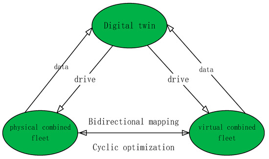
Figure 1. Structure of the integration of the virtual and real integration combined vehicle fleet.

3.2. Vehicular Networking Architecture

The main aim of the digital twin-based on-board network is to rebuild a digital united fleet in the network digital space that matches with the real united fleet. By constructing a complex system of one-to-one correspondence, cooperative interaction, and intelligent control between the physical and digital united fleets, the digital fleet can run in parallel with the physical fleet. Through the virtual service reality, data-driven governance, and the intelligent definition of everything, a new model of an on-board network is formed, in which the physical and the virtual united fleets coexist with each other in the information dimension. The on-board network architecture is shown in Figure 2.

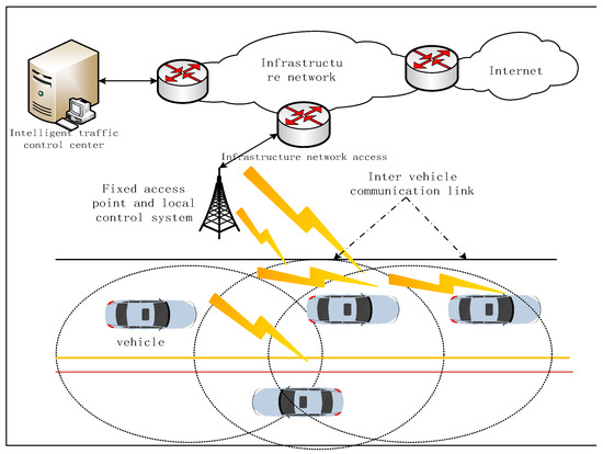
Figure 2. Vehicular networking architecture diagram.

When digital twins face different application objects, the specific system construction is different. Figure 3 presents the system architecture diagram of vehicular networks based on a digital twin, and Figure 4 shows the physical entity and the digital twin. In the physical world, the vehicle delay information is transmitted to the virtual world, where the prediction is made; the prediction results are then fed back to the vehicles in the physical world, so as to achieve the optimized outcomes. Figure 5 shows the simulation results of deep network training.

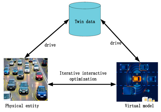
Figure 3. Architecture of the vehicular network system based on digital twins.

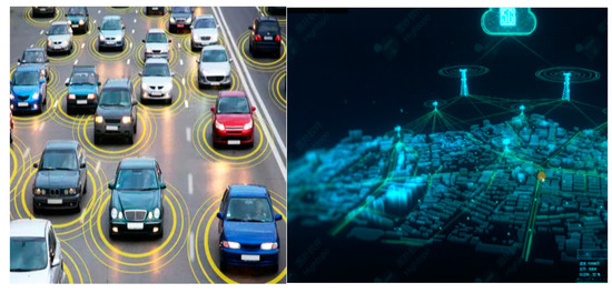
Figure 4. Physical world and digital twins.

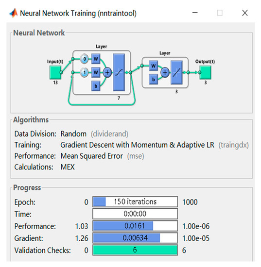
Figure 5. The simulation results of deep network training.

3.3. Network Latency Prediction Method Based on Digital Twin Technology

Network latency is a major factor affecting the performance of vehicle-mounted networked control systems. To improve the performance of vehicular-mounted networked control systems, it is crucial to know the network latency in advance, and the accuracy of network latency prediction directly affects the performance of networked control systems.

Compared with traditional communication methods, the Internet is a public transmission channel, that allows users of different terminals to share network resources to simultaneously transmit data information. In the current network environment, the data transmission rate is related to the working mechanism of the network and the network bandwidth, The data transmission rate varies greatly with the size of the data transmission and the network load, which leads to variable, uncertain, and large delays.

Therefore, in this study, a large quantity of vehicular network latency data was obtained by adopting digital twin and physical information fusion technologies. The autocorrelation of vehicle-mounted network latency was verified, and an ARMA time series model was used to carry out stationarity and residual error tests. For the verified data, the RBF and Elman neural networks were used to predict the network latency, and the prediction results are analyzed and explained. This research provides a certain reference value for the application of digital twins and the improvement in vehicle network performance.

4. Vehicle Network Physical Field Information Checking Algorithm

Using a digital twin, a vehicular network model having 25 nodes was constructed. All of the nodes in the network are mobile, and the latency data generated in the physical entity of the vehicular network are transmitted to the virtual twin. The delay statistical results are shown in Figure 6, where the x-axis is the running time and the y-axis is the corresponding time delay.

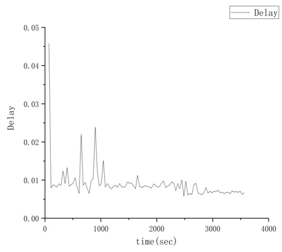
Figure 6. Time delay data of the vehicular network.

4.1. Network Latency Autocorrelation

Autocorrelation is a characteristic used to confirm the randomness of datasets, and describes the similarity between adjacent data or data separated by a certain number.

Time delay sequences are usually white noise sequences. In order to obtain a stationary time delay sequence, it is necessary to obtain its first-order differential sequence. The first-order difference equation is shown as follows:

$$\Delta X_t=X_t-X_{t-1}.$$

(1)

The time delay differential sequence is illustrated in Figure 7.where the x-axis is the time series and the y-axis is the first-order difference sequence.

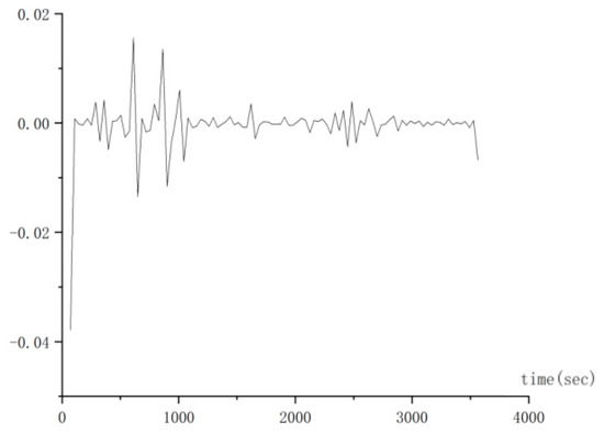
Figure 7. First-order difference sequence with time delay.

In order to better determine the stationarity of the time delay first-order difference sequence, the obtained difference sequence is divided into 11 groups, with 9 samples in each group, enabling the mean series shown in Figure 8 to be obtained.

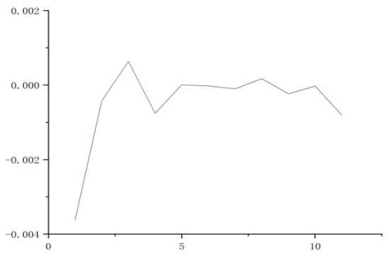
Figure 8. Mean value of first-order difference sequence.

In Figure 8, the x-axis is the number of partitions and the y-axis is the partition mean. The figure shows that the average value of each group of samples is mostly around 0, so it can be considered that the first-order difference sequence with network latency is a stationary sequence having a mean value of 0.

The autocorrelation test is conducted by testing the autocorrelation of latency values at different times before and after the network. Considering arbitrary latency sequences Y₁, Y₂, … Y_n, assuming that the sequences are stationary, the autocorrelation function r_k is estimated for several different latencies k = 1, 2, 3, etc. The time delay sequence is divided into sample sets at k intervals, i.e., the sample correlation coefficients between (Y₁, Y_1+k), (Y₂, Y_2+k), … (Y_n−k, Y_n). Because of the stationarity, the sequence has constant mean and variance. Therefore, the following sample autocorrelation function r_k is established:

$$r_k=\frac{{\displaystyle \sum _{t=k+1}^n(Y_t-\stackrel{\_}{Y})(Y_{t-k}-\stackrel{\_}{Y})}}{{\displaystyle \sum _{t=1}^n{(Y_t-\stackrel{\_}{Y})}^2}}.$$

(2)

According to Equation (2), the sample autocorrelation coefficient shown in Figure 9 can be obtained.

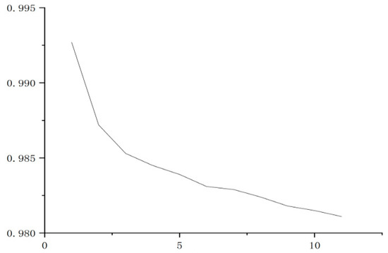
Figure 9. Sample autocorrelation coefficient.

In Figure 9, the x-axis is the lag interval and the y-axis is the sample autocorrelation coefficient. The figure shows that the time delay correlation between two adjacent moments is the strongest, and the correlation decreases with the increase in the time delay. In general, there is a strong correlation between the current period delay and the previous period delay, and there is a strong correlation between the time delay at a certain time and the time delay in the previous period. This provides a certain basis for time delay prediction, as discussed below.

4.2. ARMA

4.2.1. ARMA Time Series

Assuming that the influencing factors are $x_1,x_2,x_3,\dots x_k$, the regression analysis is as follows:

$$Y_t={\beta }_1{x}_1+{\beta }_2{x}_2+{\beta }_3{x}_3+\dots +{\beta }_p{x}_p+Z$$

(3)

where Y is the observed value, and Z is the error.

Through analysis and calculation, the ARMA model can be expressed as:

$$Y_t={\beta }_1{Y}_{t-1}+{\beta }_2{Y}_{t-2}+\dots +{\beta }_p{Y}_{t-p}+{\epsilon }_t+{\alpha }_2{\epsilon }_{t-2}+\dots +{\alpha }_q{\epsilon }_{t-q}$$

(4)

These is an ARMA(p,q) sequence.

From Equation (4), it is assumed that the sequence $\{Y_t,t=0,\pm 1,\pm 2,\dots \}$ satisfies the following.

$$Y_t-{\beta }_1{Y}_{t-1}-{\beta }_2{Y}_{t-2}-\dots -{\beta }_p{Y}_{t-p}={\epsilon }_t-{\alpha }_1{\epsilon }_{t-1}-\dots -{\alpha }_q{\epsilon }_{t-q}$$

(5)

where Y_t is a zero-mean stationary sequence, and ${\epsilon }_t$ is smooth white noise, Then, Y_t is an ARMA sequence having order p and q.

For the general stationary sequence $\{Y_t,t=0,\pm 1,\pm 2,\dots \}$, E(Y_t) = μ, then:

$${(Y}_t-\mu )-{\beta }_1(Y_{t-1}-\mu )-\dots -{\beta }_p(Y_{t-p}-\mu )={\epsilon }_t-{\alpha }_1{\epsilon }_{t-1}-\dots -{\alpha }_q{\epsilon }_{t-q}$$

(6)

4.2.2. ARMA Verification

• Stationarity verification

In this paper, ADF verification and KPSS verification are used.

Using MATLAB to calculate the original data, we obtain:

y_h_adf = 1

y_h_kpss = 0.

Thus, it is proved that the original sequence is a stationary one.

2.

Determine the ARMA model order

The purpose of the Akaike Information Criterion (AIC) criterion is to select p and q so that

$$\min AIC=n\ln n{\widehat{\sigma }}_{\epsilon }^2+2(p+q+1)$$

(7)

In Equation (7), n represents the size of the selected samples, and ${\widehat{\sigma }}_{\epsilon }^2$ represents the expected value. AIC has a minimum value when $p=\widehat{p}$,$q=\widehat{q}$, and it is considered that ARMA($\widehat{p},\widehat{q}$) has the best stationarity.

When the ARMA(p,q) sequence contains μ, the model is $\mathrm{\Phi }(B)(X_t-\mu )=\theta (B)\epsilon$. At this time, k = p + q + 2, and the AIC criterion is expressed as: select p,q, so that we have

$$\min AIC=n\ln n{\widehat{\sigma }}_{\epsilon }^2+2(p+q+2)$$

(8)

The minimum points of Equations (7) and (8) are the same, i.e., $\widehat{p},\widehat{q}$.

3.

Residual verification

To ensure the proper order, a residual test is also required. If the residuals are randomly normally distributed and uncorrelated, they represent a white noise signal, indicating that this model is effective. On the contrary, if the residuals are not randomly normally distributed and uncorrelated, the model is not effective enough.

Through analysis and calculation, the residual test results are shown as follows. Figure 10, Figure 11, Figure 12 and Figure 13 plot the residual test results. The above verification demonstrates that the residual is close to a normal distribution and the mean value is 0. There are no points beyond the blue line in the ACF and PACF graphs, which indicates that the residuals is are uncorrelated and represent a white noise signal.

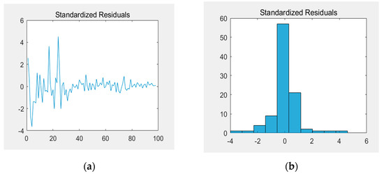
Figure 10. Standardized residuals. (a) Standardized residual; (b) Standardized residual.

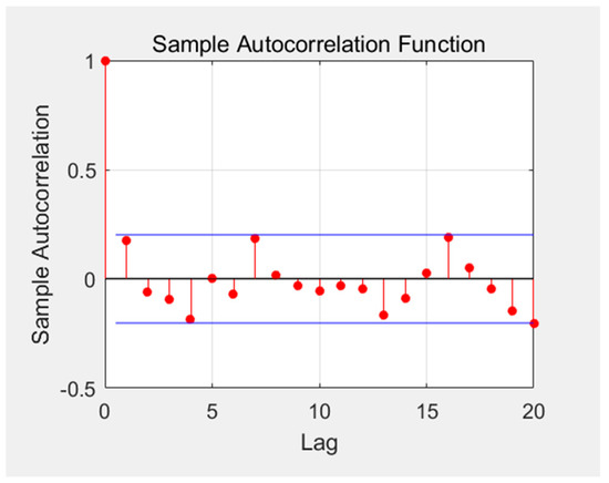
Figure 11. ACF function diagram.

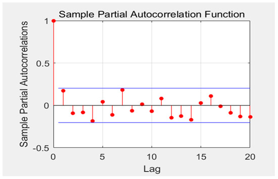
Figure 12. PACF function.

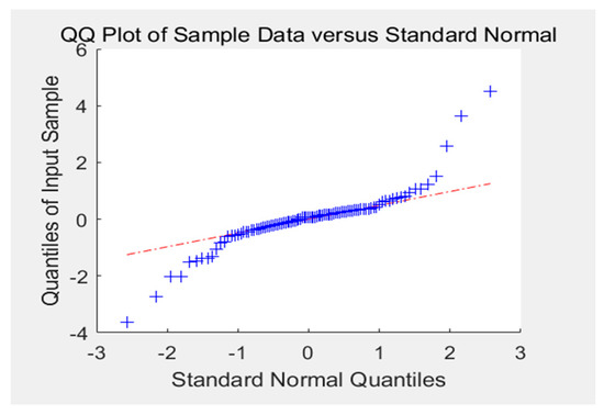
Figure 13. Residual QQ.

5. Latency Prediction Algorithm Based on Neural Networks

Artificial neural networks have strong advantages in tackling the problem of latency prediction. Data transmission delays in vehicular networks are neither random in nature, or unpredictable. Within a certain range of time, from the above research and analysis, it can be found that the transmission delay of the network has strong autocorrelation, and there is a certain nonlinear relationship between the network latency at the next time-step and that of the preceding time-step. Furthermore, the latency in the whole local range fluctuates with in an interval, showing the characteristics of nonlinear change; that is, the network latency is characterized by locality, nonlinearity, and autocorrelation.

5.1. Composition Method of Training Samples and Samples to Be Predicted

Through the previous analysis, it can be found that the latency variation in vehicular networks has certain regularity, and the latency can be predicted by summarizing its regularity. Therefore, according to the latency data obtained from network latency measurement, the collected latency data are divided into several time segments in sequence. One of the points T is selected, and the N number x values (latency) obtained before this timestep are used to estimate the x value of the T + d time point, thus realizing the prediction of time series, namely:

$$X_{T+d}=f(x_{T-n+1},x_{T-n+2},x_{T-n+3},\dots ,x_T)$$

(9)

where d is usually one, so that the value of x in the time-step after following T can be predicted according to function f().

In this paper, the 1st to 8th latency values are taken as input sample 1, and the 9th latency value is taken as output sample 1, forming a sample pair. Then, the 2nd to 9th latency values constitute input sample 2, and the 10th latency value constitues output sample 2, totaling 90 samples.

5.2. Data Preprocessing

After determining the training samples and the samples to be predicted, the mapminmax function of MATLAB was invoked to normalize the data. This is because normalization can prevent the overflow of computation in the training process and accelerate the convergence speed in the learning and training processes.

5.3. Latency Prediction Based on RBF

5.3.1. RBF Network

The RBF network has a fast training speed and a strong nonlinear mapping function. The hidden layer uses a Gaussian radial basis function as the excitation function, as shown in Figure 14. Figure 15 shows the RBF neural network model structure.

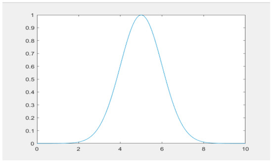
Figure 14. Gaussian radial basis function.

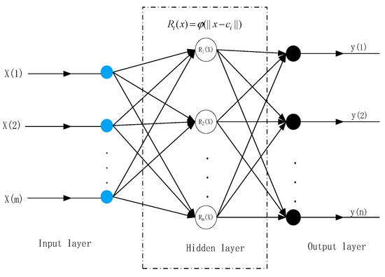
Figure 15. RBF neural network model structure.

The activation function of the hidden layer node produces a localized response to the input excitation. The output response of each hidden layer node is

$$R_i(x)=𝜑(\Vert x-c_i\Vert )$$

(10)

Inside:

$$𝜑(\Vert x-c_i\Vert )=\exp (-\frac{\Vert x-c_i|{|}^2}{2{\sigma }_i^2}),i=1,2,\dots ,m$$

(11)

In Equation (11),where x is the m-dimensional input vector; $c_i$ is the center of the i-th basis function; $\sigma$ is a freely selectable parameter that determines the width of the basis function; l is the number of hidden layer nodes; $\left|\right|x-c_i\left|\right|$ is the norm of vector $(x-c_i)$, which represents the distance between x and $c_i$; and R_i(x) is the response of the i-th basis function to the input vector. There is a unique maximum value at $c_i$, and, as $\left|\right|x-c_i\left|\right|$ increases, $R_{i(x)}$ decays quickly to zero. The input layer realizes the nonlinear mapping from x to $R_{i(x)}$, and the output layer realizes the linear mapping from $R_{i(x)}$ to $y_k$, namely:

$$y_k={\displaystyle \sum _{i=1}^l{w}_{ik}}{R}_i(x),k=1,2,\dots ,n,$$

(12)

In Equation (12), where $y_k$ is the response level; $w_{ik}$ is the weight; and n is the number of output layer nodes, and n = 1.

The output layer is used to generate the final model prediction result according to the weight matrix.

The RBF parameters are determined as follows:

• Radial basis function center: the main methods used are the self-organized selection center method and the orthogonal least square method.
• Determine the width of the neurons in the hidden layer of RBF. This is determined by the KNN algorithm, as follows:

$${\sigma }_i=\frac{1}{k}{\displaystyle {\sum }_{j-1}^k\Vert v_i-v_j\Vert }$$

(13)

where k is a constant, and v_j (j = 1,2,…,k) represents the center closest to the i-th center v_i.

3.

Determine the weight of the output layer.

The approximation function of the RBF is:

$$F(x)={\displaystyle {\sum }_{i=1}^c{w}_i}G(\Vert x-v_i\Vert )$$

(14)

where v_i is the clustering center, G(x) is the Gaussian function, and $\Vert \cdot \Vert$ is the Euclidean norm. We have the following cost function:

$$\begin{array}{l}\psi (F*)={{\displaystyle {\sum }_{k=1}^n[d_k-F(x_k)]}}^2+\lambda {\Vert DF*\Vert }^2\\ ={{\displaystyle {\sum }_{k=1}^n[d_k-{\displaystyle {\sum }_{i=1}^c{w}_{i}G(\Vert x_k-v_i\Vert )}]}}^2+\lambda {\Vert DF*\Vert }^2\end{array}$$

(15)

where ${{\displaystyle {\sum }_{k=1}^n[d_k-F(x_k)]}}^2$ is the standard error and $\lambda \Vert DF*\Vert$ is the regularization, which includes the requirements for smoothness and continuity.

$$\begin{array}{ll}\psi (F*)& ={{\displaystyle {\sum }_{k=1}^n[d_k-GW]}}^2+\lambda {(DF*,DF*)}_N^2\\ & ={\Vert d-GW\Vert }^2+\lambda w^T{G}_{0}W\end{array}$$

(16)

Inside:

$$w={(w_1,w_2,\dots ,w_c)}^T$$

(17)

$$d=\left[\begin{array}{cccc}G(x_1,v_1)& G(x_1,v_2)& \cdots & G(x_1,v_c)\\ G(x_2,v_1)& G(x_2,v_2)& \cdots & G(x_2,v_c)\\ ⋮& ⋮& ⋮& ⋮\\ G(x_n,v_1)& G(x_n,v_2)& \cdots & G(x_n,v_c)\end{array}\right]$$

(18)

Minimize $\psi (F*)$ to obtain:

$$(G^{T}G+\lambda G_0)w=G^{T}d$$

(19)

Normalization:

$$w={(G^{T}G+\lambda G_0)}^{-1}{G}^{T}d$$

(20)

The iterative process is:

$$w_{k+1}=w_k-[(G^{T}G+\lambda G_0)w_k-G^{T}d]$$

(21)

5.3.2. Vehicular Network Latency Prediction

We used the newrb function in MATLAB to generate an RBF neural network, as follows:

$$net=newrb(p_n,t_n,goal,spread,mn,df)$$

where $p_n,t_n$ are the normalized input and output samples, respectively; ‘goal’ is the mean square error; mn is the largest number of neurons in the hidden layer; ‘spread’ is the distribution of the function; and df is the number of neurons added to the display. Figure 16 depicts the flow chart of RBF neural network prediction.

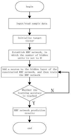
Figure 16. Flowchart of RBF neural network prediction.

When using the RBF network to approximate the function, The network output at this time is:

$$An=sim(net,p_n)$$

The output value needs to be denormalized to obtain the predicted actual value.

Figure 17 shows the prediction confidence interval graph. Where the x-axis is the time and the y-axis is the delay. The red line is the 95% confidence interval. For comparison, Figure 18 shows the prediction and actual latency of the RBF neural network. where the x-axis is the running time and the y-axis is the corresponding time delay. Figure 19 shows the errors between the actual and predicted values. where the x-axis is the running time and the y-axis is the corresponding time delay. When the network latency is relatively stable, using the RBF neural network to predict the latency can achieve a higher prediction accuracy. More than 95% of the prediction values have an error within 5%.

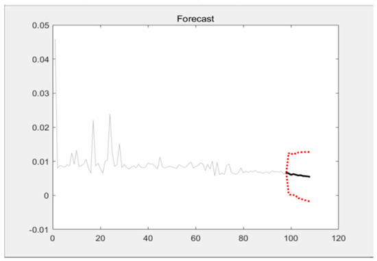
Figure 17. Confidence interval of the predicted value.

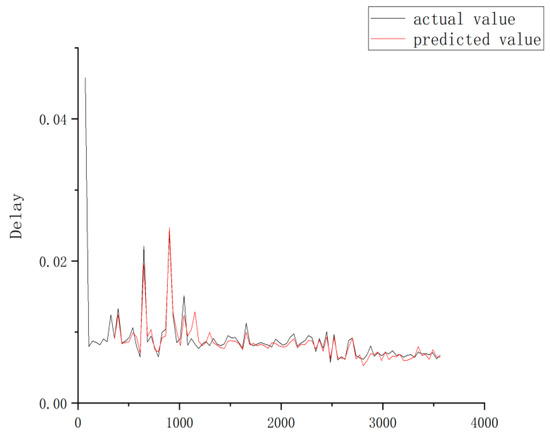
Figure 18. Comparison of the actual and predicted values.

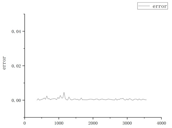
Figure 19. Error between the actual and predicted values.

5.4. Latency Prediction Based on Elman

5.4.1. Elman Network

The main structure of the Elman neural network comprises feedforward connections. Figure 20 shows the Elman network structure.

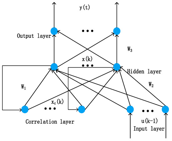
Figure 20. Structure diagram of the Elman network.

The input layer has r nodes, the hidden layer and correlation layer have n nodes, and the output layer has m nodes; the mathematical model of the network can then be given by:

$$x(k)=f(W^1{x}_c(k)+W^{2}u(k-1))$$

(22)

$$x_c(k)=\alpha x_c(k-1)+x(k-1),0\le \alpha <1$$

(23)

$$y(k)=g(W^{3}x(k))$$

(24)

where them: $f(x)$ is the sigmoid function as follows:

$$f(x)=\frac{1}{1+e^{-x}},0\le \alpha <1$$

(25)

Then:

$$y(k)=W^{3}x(k)$$

(26)

The Elman learning algorithm can be derived from $\Delta W=-\eta \frac{\partial E}{\partial W}$ as follows:

$$\begin{array}{l}\Delta W_{ij}^3={\eta }_3{\delta }_i^0{x}_j(k),i=1,2\dots ,m;j=1,2,\dots ,n\\ \Delta W_{jq}^2={\eta }_2{\delta }_j^h{U}_q(k-1),j=1,2\dots ,n;q=1,2,\dots ,r\\ \Delta W_{jt}^1={\eta }_1{\displaystyle \sum _{i=1}^m({\delta }_i^0{w}_{ij}^3)}\frac{\partial X_j(k)}{\partial w_{jt}^1},j=1,2\dots ,n;t=1,2,\dots ,n\end{array}$$

(27)

where ${\eta }_1,{\eta }_2,{\eta }_3$ are the learning step lengths of $W^1,W^2,W^3$, respectively.

5.4.2. Vehicular Networking Latency Prediction

First, the network is initialized, including the number of neurons in each layer, learning efficiency, and training error, Second, the sample value of the experiment is used to calculate the output value and training error of each layer, It can and then be decided whether the training error meets the requirements or reaches the maximum number of training steps. If so, the training is over. Otherwise, the training is continued, and the network parameters are continuously updated until the conditions are met. The Elman training process is shown in Figure 21.

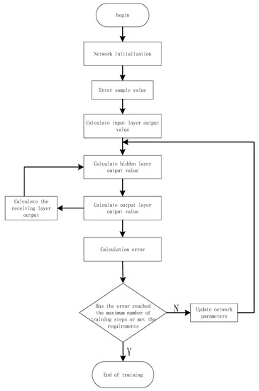
Figure 21. Training process of the Elman neural network.

Using experimental data, Figure 22 compares the actual and predicted values, and Figure 23 shows the discrepancy between the two.

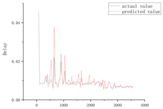
Figure 22. Comparison of the actual and predicted values.

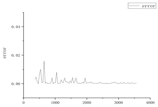
Figure 23. Error between the actual value and predicted values.

As can be seen from Figure 23, most of the actual values are quite different from their, predicted counterparts, and only a few of the predicted values are close to the true values. Therefore, the performance of the prediction model based upon the Elman neural network is poor.

5.5. Complexity Analysis of RBF and Elman Models

The RBF neural network is a type of local approximation network, that can accurately approximate any continuous function. It has a fast training speed and a strong nonlinear mapping function. It is a three-layer feedforward network having a single hidden layer. The model is composed of three parts, namely, an input layer, a hidden layer and an output layer. The hidden layer uses a Gaussian radial basis function as the excitation function; The hidden layer is to maps the vector from the low dimension to the high dimension, so that low-dimension linear separability becomes high-dimension linear separability. The output layer is used to calculate their linear combination. Therefore, the complexity of the RBF network model is Q(n²).

The Elman neural network is a typical dynamic recurrent neural network. Its main structure comprises is feedforward connections, including an input layer, hidden layer(s), and an output layer. Its connection weights can be learned and modified. The feedback connection is composed of a group of structural units to remember the output value of the previous time period. In this network, in addition to the ordinary hidden layer, there is a special hidden layer, which is called the association layer (or association unit layer), This layer receives the feedback signal from the hidden layer, and each hidden layer node is connected with a corresponding association layer node. The function of the correlation layer is to take the hidden layer state of the previous time period together with the network input of the current period time as the input of the hidden layer through the connection memory, which is equivalent to state feedback. The transfer function of the hidden layer is still a nonlinear function, (generally, a sigmoid function), and the output layer and the correlation layers are also linear functions. Therefore, the complexity of the Elman network model is Q(nlogn).

Compared with the Elman network complexity of O(nlogn), the complexity of the RBF network O(n²) is larger. The smaller the network complexity is, the shorter the execution time and frequency of the algorithm is, and the better the algorithm is. Therefore, the Elman network is considered to be superior to its RBF counterpart.

5.6. Comparative Analysis of Model Results

As can be seen from Figure 24, Through analysis and calculation, it was found that the average latency of the actual vehicular network is 0.00897, the RBF prediction is 0.00839, the average error rate is 0.00069, and the average relative error rate is 7.6%; the average prediction latency using the Elman network is 0.00906 s, the average error rate is 0.00128, and the average relative error rate is 14.2%. Therefore, in terms of the latency prediction for the vehicular network, the RBF network outperforms its Elman peer. According to the RMS calculation equation, it was found that the actual vehicle network delay RSM is 0.00901, the RBF neural network prediction delay RSM is 0.00897, and the Elman neural network prediction delay RSM is 0.00962 as shown in Table 1.

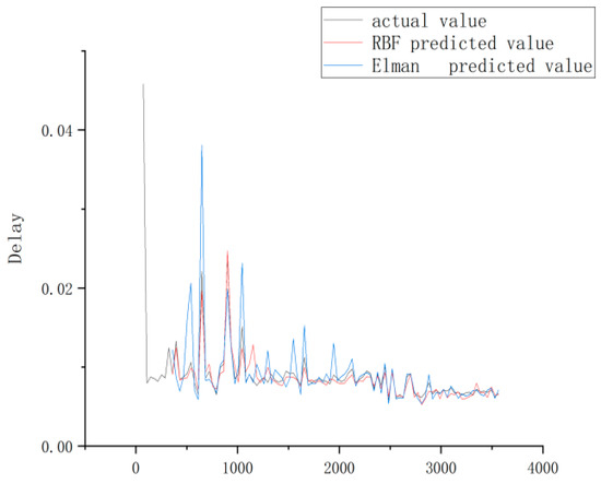
Figure 24. Comparison of latency prediction results based upon the RBF and Elman networks.

Table 1. RSM value comparison.

Attribute	Actual	RBF	Elman
RMS	0.00901	0.00897	0.00962

6. Conclusions

With the aid of digital twin technology, the RBF and Elman neural networks awere employed for the online prediction of the uncertain vehicular network latency online, and the MATLAB software is was used to perform simulationse. Because the RBF has good global approximation performance, and nonlinear mapping ability, and highly non-linear characteristics, the latency data of the vehicular network based on analysis and calculation is represent a type of time series with having strong non-linearity. Since a neural network model needs to use historical latency information to predict future latency, digital twins technology was employed. A large amount of latency data was collected through the actual network latency measurement, and the latency autocorrelation is was analyzed and verified. Finally, a latency prediction model was constructed based on RBF and Elman neural networks to predict the latency of the vehicular network. It can be concluded from the presented simulation result that for the prediction of stable latency, the proposed method achieves a good prediction performance and offers a good real-time performance. It This research provides a certain reference value for the application of digital twins and latency performance optimization of vehicular networks.

References

- Fei, T.; He, Z. Ten Questions about Digital Twins: Analysis and Thinking. Comput. Integr. Manuf. Syst. 2020, 26, 1–17. [Google Scholar]
- Cheng, J.; Zhang, H.; Tao, F.; Juang, C.F. DT-II: Digital twin enhanced Industrial Internet reference framework towards smart manufacturing. Robot. Comput.-Integr. Manuf. 2020, 62, 101881. [Google Scholar] [CrossRef]
- Negri, E.; Fumagalli, L.; Macchi, M. A Review of the Roles of Digital Twin in CPS-based Production Systems. Procedia Manuf. 2017, 11, 939–948. [Google Scholar] [CrossRef]
- Fei, T.; Ying, C.; Cheng, J.; Zhang, M. Theories and technologies of cyber-physical fusion in digital twin workshop. Comput. Integr. Manuf. Syst. 2017, 23, 1603–1611. [Google Scholar]
- Jiang, Y.; Ding, G.; Zhang, J. The evolution mechanism and operation mechanism of digital twin workshop. China Mech. Eng. 2020, 31, 824–832+841. [Google Scholar]
- Liu, K.; Wang, P.; Liu, T. The application of digital twin in the operation and maintenance of aero-engine. Aviat. Power 2019, 4, 70–74. [Google Scholar]
- Guo, J.; Hong, H.; Zhong, K.; Liu, X.; Guo, Y. Production control method of aerospace manufacturing workshop based on digital twin. China Mech. Eng. 2020, 31, 808–814. [Google Scholar]
- Aivaliotis, P.; Georgoulias, K.; Chryssolouris, G. The use of Digital Twin for predictive maintenance in manufacturing. Int. J. Comput. Integr. Manuf. 2019, 32, 1067–1080. [Google Scholar] [CrossRef]
- Shevlyugin, M.V.; Korolev, A.A.; Golitsyna, A.E.; Pletnev, D.S. Electric Stock Digital Twin in a Subway Traction Power System. Russ. Electr. Eng. 2019, 90, 647–652. [Google Scholar] [CrossRef]
- Lopes, M.R.; Costigliola, A.; Pinto, R.; Vieira, S.; Sousa, J.M. Pharmaceutical quality control laboratory digital twin—A novel governance model for resource planning and scheduling. Int. J. Prod. Res. 2020, 58, 6553–6567. [Google Scholar] [CrossRef]
- Killat, M.; Hartenstein, H. An Empirical Model for Probability of Packet Reception in Vehicular Ad Hoc Networks. EURASIP J. Wirel. Commun. Netw. 2009, 2009, 721301. [Google Scholar] [CrossRef] [Green Version]
- Zorzi, M. Data-link packet dropping models for wireless local communications. IEEE Trans. Veh. Technol. 2002, 51, 710–719. [Google Scholar] [CrossRef]
- Lai, W.; Ni, W.; Wang, H.; Liu, R.P. Analysis of Average Packet Loss Rate in Multi-Hop Broadcast for VANETs. IEEE Commun. Lett. 2018, 22, 157–160. [Google Scholar] [CrossRef]
- Fu, Y.; Wang, Z.; Su, Y.; Dai, F.; Zhong, L.; Guo, D. Availability modeling of military Ad hoc networks based on Markov chains. J. Mil. Eng. 2021, 42, 65–73. [Google Scholar]
- Liu, Y. Research on Packet Loss Characteristics in Vehicle Self-Organizing Network. Ph.D. Thesis, Tianjin University of Technology, Tianjin, China, 2019. [Google Scholar]
- Fan, M.; Jiang, H.; Ding, G.; Wang, B. Metro Train Performance Evaluation System Based on Digital Twin. Comput. Integr. Manuf. Syst. 2021, 7, 1–18. [Google Scholar]
- Hassanabadi, B.; Shea, C.; Zhang, L.; Valaee, S. Clustering in Vehicular Ad Hoc Networks using Affinity Propagation. Ad Hoc Netw. 2014, 13, 535–548. [Google Scholar] [CrossRef]
- Qie, G.; Zhang, Y. Analysis of Smart Car and Networking Technology. Mob. Commun. 2020, 44, 80–85. [Google Scholar]
- Fang, K.; Zhu, C.; Liu, D. Innovative Application Research of 5G Technology in the Automobile Industry. Technol. Innov. 2020, 4, 148–149. [Google Scholar]
- Li, K.; Dai, Y.; Li, S. Development status and trend of intelligent networked vehicular (ICV) technology. J. Automot. Saf. Energy Conserv. 2017, 8, 1–14. [Google Scholar]
- Xun, Y.; Liu, J.; Zhao, J. Research on the Security Threats of Intelligent Connected vehiculars. J. Internet Things 2019, 3, 72–81. [Google Scholar]
- Lv, Y.; Zhai, Y.; Li, P. Research on the New vehicle Network Architecture Based on SDN. J. Hubei Inst. 2021, 35, 27–33. [Google Scholar]
- Yang, J.; Dou, J. Simulation analysis of high-speed Ethernet time delay. Comput. Sci. 2011, 38 (Suppl. S1), 341–344. [Google Scholar]
- Zhang, Y. Performance Research and Application of EtherNet/IP Industrial Ethernet. Ph.D. Thesis, Beijing Jiaotong University, Beijing, China, 2016. [Google Scholar]
- Lei, H.; He, D.; Miao, J. Analysis of On-board Ethernet latency of High-speed EMUs. Comput. Meas. Control. 2013, 21, 1320–1322. [Google Scholar]
- Zhang, L. Research on real-time performance of industrial Ethernet. Gansu Sci. Technol. 2010, 26, 25–26. [Google Scholar]
- Zhou, G.; Wang, H. Analysis and Modeling of Industrial Ethernet Performance. Instrum. Technol. Sens. 2013, 02, 95–97. [Google Scholar]
- Miao, J.; He, D.; Ding, C. Research on Train Communication Network and Simulation Based on Industrial Ethernet. Comput. Meas. Control. 2010, 18, 2417–2420. [Google Scholar]
- Pei, Z. Research on the Performance of Ethernet-Based Train Communication Network. Ph.D. Thesis, Southwest Jiaotong University, Chengdu, China, 2014. [Google Scholar]
- Chen, X.; Liu, J.; Fu, S. Analysis of the Transmission latency Characteristics of Industrial Ethernet. Comput. Inf. Technol. 2007, 4, 63+66. [Google Scholar]
- Lu, T.; Wang, W. vehicle network cluster routing algorithm based on genetic characteristics. Comput. Technol. Dev. 2021, 31, 13–18. [Google Scholar]
- Jin, H.; Zhong, C. Real-time Ethernet buffer queue optimization algorithm based on queuing theory. J. Dalian Univ. Technol. 2012, 52, 95–99. [Google Scholar]
- Niu, Z. Research on latency Compensation in Ethernet Frame Transmission. Comput. Netw. 2008, 34, 52–54+65. [Google Scholar]
- Huang, L. Investigation on the Status and Development of Automotive Ethernet Technology. J. Sci. Technol. Econ. 2019, 27, 22+24. [Google Scholar]
- Yang, H.; Qin, G.; Yu, H.; Wang, Y. Summary of vehicle-mounted time-sensitive network technology. Comput. Appl. Softw. 2015, 32, 1–5+10. [Google Scholar]
- Guo, L.; Chen, X. Application of Ethernet Technology in Automobile Communication. AutomotiveElectrics 2017, 6, 36–38+42. [Google Scholar]
- Tan, Y. Explore the application of Ethernet technology in automobile communication. Digit. Commun. World 2019, 2, 211. [Google Scholar]
Publisher’s Note: MDPI stays neutral with regard to jurisdictional claims in published maps and institutional affiliations. |
© 2022 by the authors. Licensee MDPI, Basel, Switzerland. This article is an open access article distributed under the terms and conditions of the Creative Commons Attribution (CC BY) license (https://creativecommons.org/licenses/by/4.0/).