Article

A Lightweight Method for Vehicle Classification Based on Improved Binarized Convolutional Neural Network

1
Faculty of Information Engineering and Automation, Kunming University of Science and Technology, Kunming 650500, China
2
Yunnan Key Laboratory of Computer Technologies Application, Kunming University of Science and Technology, Kunming 650500, China
*
Author to whom correspondence should be addressed.
Electronics 2022, 11(12), 1852; https://doi.org/10.3390/electronics11121852
Submission received: 27 April 2022 / Revised: 28 May 2022 / Accepted: 6 June 2022 / Published: 10 June 2022

Abstract

:
Vehicle classification is an important part of intelligent transportation. Owing to the development of deep learning, better vehicle classification can be achieved compared to traditional methods. Contemporary deep network models have huge computational scales and require a large number of parameters. Binarized convolutional neural networks (CNNs) can effectively reduce model computational size and the number of parameters. Most contemporary lightweight networks are binarized directly on a full-precision model, leading to shortcomings such as gradient mismatch or serious accuracy degradation. To addresses the inherent defects of binarization networks, herein, we adjust and improve residual blocks and propose a new pooling method, which is called absolute value maximum pooling (Abs-MaxPooling). The information entropy after weight binary quantization is used to propose a weight distribution binary quantization method. A binarized CNN-based vehicle classification model is constructed, and the weights and activation values of the model are quantified to 1 bit, which saves data storage space and improves classification accuracy. The proposed binarized model performs well on the BIT-Vehicle dataset and outperforms some full-precision models.

1. Introduction

The number of urban vehicles has been increasing every year; to efficiently manage traffic, the traffic monitoring information system of each city is being continuously improved. Image-based vehicle classification technology has become a popular research topic in the intelligent transportation domain.
Convolutional neural networks (CNNs) have greatly improved vehicle classification accuracy; however, complex CNN models based on floating-point multiplication operations, such as VGG [1] and ResNet [2], have huge computational scales and require a large number of parameters. These models consume a large amount of computational and memory resources, which seriously hinders their application in small devices. A binarized neural network (BNN) [3] can be used to quantize 32-bit floating-point parameters into 1-bit fixed-points. Moreover, the large number of floating-point multiplication and addition operations in CNNs can be converted into more efficient logic operations (such as XNOR and POPCOUNT) owing to the 1-bit advantage. It decreases the consumption of storage resources for model deployment as well as the computational load of the model, greatly accelerating the forward inference process of the neural network. Because of the high compression ratio and acceleration effect, BNNs have received considerable attention in recent years and are a popular research topic in the study of lightweight deep learning models.
Contemporary BNNs need improving in the following areas [4,5,6]: (1) The current lightweight method of direct binarization of full-precision networks does not consider the weak information representation of the binarized model, which leads to a less rich information flow of the binarized network; moreover, the downsampling layer introduces a large number of 1 × 1 floating-point convolutions to expand the number of channels, adding too many additional floating-point parameters and calculations. (2) The existing binarization network backpropagation process only considers the approximation of the symbolic function, ignoring the problem that the parameters cannot be updated effectively in some intervals; there is also a serious gradient mismatch problem. (3) Most reported methods recover the loss of weight quantization by introducing floating-point scaling; however, this operation introduces additional floating-point parameters and computations, which increases the storage and operation burden of binarized CNNs.
Based on the above analysis, the contributions of this study are as follows:
(1)
Based on absolute value maximum pooling, we propose a downsampling method. The residual block of ResNet is adjusted and improved to make it more suitable for binary CNNs. In the pooling operation, the value with the largest absolute value in each pooling block is retained, and thus, the information of the feature map after binary quantization is retained more effectively. Such a downsampling layer does not require a full-precision convolution operation, which greatly reduces the number of floating-point operations used in the model.
(2)
For approximating the gradient of the symbolic function, a dynamic and progressive method is proposed that approximates the backpropagation gradient of the binarization function step-by-step during training. This method is used to more efficiently train the binarized CNN, addressing the problem that the model parameters cannot be updated in some intervals. The gradient of the later period gradually approaches the gradient of the symbolic function, considerably mitigating the gradient mismatch problem.
(3)
Herein, an information gain method is proposed, which is called the binarization of weight redistribution. The full-precision weights are standard deviation normalized before the weights are binarized. Floating-point gain terms that are introduced in most networks to reduce binary quantization errors are discarded, which enhances the information representation capability of the binary network and decreases the storage and operation burden of the traditional floating-point scaling gain.
The rest of the paper is organized as follows: Section 2 presents a review of current research on binarized CNNs and vehicle classification and analyzes the current problems. Section 3 details the proposed improvement method. In Section 4, the improved residual blocks are used with the cifar10 dataset [7]; the experimental results demonstrate the effectiveness of our proposed improvement. Subsequently, extensive experiments are conducted on the BIT-Vehicle public dataset [8], and the experimental results show that the proposed binarized CNN model outperforms contemporary binarized models, as well as the partial full-precision CNN.

2. Related Works

2.1. Binarized Convolutional Neural Networks

In full-precision CNNs, the weights and activation values are 32-bit floating-point numbers. In forward inference, the convolutional operation contains a large number of floating-point multiplication and addition operations, which causes inefficiency; moreover, the 32-bit floating-point weights occupy considerable storage space. Binarized CNNs binarize the weights and activation values into {+1, −1}, which considerably compresses the storage space and replaces the complex floating-point operations by more efficient logic operations (XNOR and POPCOUNT).
Bengio et al. proposed the first truly binarized CNN in 2016. This model binarized both weights and activations in a CNN for the first time. Since then, more advanced BNNs, such as XNOR-Net [9], Bi-Real-Net [10], IR-Net [11], and ReActNet [12], IE-Net [13], DPBNN [14], have been proposed with improved performance; these models enable real-time application of binarized CNNs. Wang et al. applied binary CNNs to wireless interference recognition. They proposed two techniques to minimize quantization noise and create multiple routes to update the parameters of BNNs for solving the bottleneck of the serious performance degradation of BNNs, resulting in further improvement in performance [15]. Qian et al. developed BNNs for speech recognition. They developed several types of BNNs and related model optimization algorithms for large vocabulary continuous speech recognition acoustic modeling, decreasing the computational cost during the inference stage [16]. Jing et al. proposed a lightweight multispectral classification method called CABNN based on BNNs that had an effective trade-off between model performance and computational cost. CABNN has higher efficiency and better comprehensive performance than several state of-the-art methods [17].

2.2. Vehicle Classification

In traditional vehicle classification methods, manually designed feature descriptors, such as scale-invariant feature transformation (SIFT), can only focus on the shallow features of an image, which requires a high-quality image, are easily affected by the background, and are not sufficiently robust. In recent years, with the continuous development of deep learning, some scholars have applied deep learning algorithms to the field of vehicle classification. In deep learning, CNNs use a large amount of data to automatically learn how to extract the depth features of an image, achieving much better classification performance than traditional methods. Hasan et al. proposed a ResNet-50-based pre-trained deep learning model for migration learning for the recognition and classification of native vehicle types in Bangladesh, which achieved an accuracy of 98.00% [18]. Habib et al. developed an optimized automatic surveillance and auditing system to detect and classify vehicles of different categories, achieving 96.04% accuracy on vehicle type classification [19]. Chen et al. proposed a novel model to classify five distinct groups of real-life vehicle images based on the AdaBoost algorithm and deep CNNs, and their performance was significantly better than that of traditional algorithms such as SIFT-SVM, HOG-SVM, and SURF-SVM [20].

2.3. Current Problems

Analysis of current research status shows that the following problems exist in the field of intelligent vehicle recognition.
(1)
In current approaches, to lighten the model by directly binarizing the full-precision network, the information flow is not sufficiently rich, and the use of 1 × 1 convolution for downsampling adds too many additional floating-point parameters and computations.
(2)
Existing approximation methods for symbolic functions of binarized networks ignore the problem that the parameters cannot be updated effectively in some cases, and there is a serious gradient mismatch problem.
(3)
The introduction of floating-point scaling in binarization networks to recover the weight quantization loss introduces additional floating-point parameters and computations, which increases the storage and operation burden of binarization CNNs.
In this study, we address these problems in binarized CNNs. We improve the model structure, training method, and weight quantization method to enable binarized CNN and achieve better results in vehicle classification tasks.

3. Methods

Unlike full-precision networks, in binarized CNNs, discrete quantization values limit their ability to learn richly distributed expressions; moreover, it is challenging for binarized networks to retain and transfer information efficiently. Furthermore, in the binarized quantization process, quantization errors occur and there is a mismatch between the gradients of forward and backward propagation during the training of binarized CNNs, decreasing the accuracy of binarized CNNs. This affects the final classification. Therefore, we address these problems and improve the accuracy of the binarized CNNs for vehicle classification by learning the effective features of information.
In this section, we describe our binarized CNN model in detail. We first describe how to improve the building blocks of ResNet to fit the binarized network for achieving higher accuracy with a more streamlined structure and propose a new pooling method in that structure. Then, a weight redistribution binarization method is used. Finally, we present how to train the binarization model more effectively.

3.1. Improved Binarized Residual Network

In network models such as VGG and GoogLeNet [21], the network accuracy saturates and even decreases, and gradient disappearance and gradient explosion occur when the network depth increases. The residual network proposed by He et al. in 2016 incorporates a residual unit for constant mapping through a short-circuiting mechanism, which can effectively solve these problems. The residual units also enhance the number of network information transfer paths, allowing effective training of deeper network models while ensuring a higher accuracy.
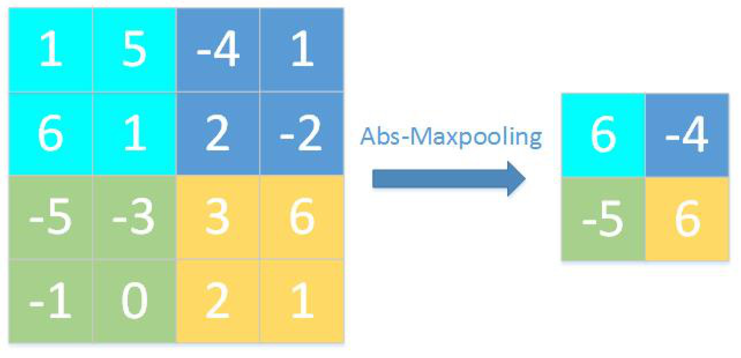
An improved residual block is illustrated in Figure 1. Unlike ResNet, in a binarized CNN, the binary quantization of activation values and weights leads to serious loss of network information; thus, we use a denser residual connection to ensure more effective retention of the information in the network and improve the expressiveness of the network. In a traditional residual network, in the downsampling layer, after full-precision 1 × 1 convolution and normalization layer to ascend and downsample, the main function is to obtain an output with the same size as the output of the convolutional output path, to not make the improvement of the network performance too obvious. In the binary quantized network, such a structure also adds additional floating-point operations; accordingly, this study proposes a new downsampling method, called absolute value maximum pooling (Abs-MaxPooling) (Figure 2), which can reserve the number with the largest absolute value in each pooling block of the input feature map.
Furthermore, the binarized convolution in the downsampling layer is not expanded by the number of channels, and the two are subsequently stitched together as the input to the next layer. Thus, the downsampling layer has fewer floating-point operations due to the 1 × 1 convolution and normalization layers, and the binary convolution kernel is reduced by a half.
For a feature map of a binary distribution, we assume that it obeys a Bernoulli distribution with a probability distribution function:
f ( x b ) = { p , 1 p , i f i f x b = + 1 x b = 1
where p is the probability of taking the value +1, p ( 1 , 1 ) , x b is the binarized value; then, the information entropy of the distribution after binarization is expressed using Equation (2):
H ( x b ) = p ln ( p ) ( 1 p ) ln ( 1 p )
For the binarized distribution to retain the maximum amount of information, the information entropy of the binarized distribution should be maximized:
max ( H ( x b ) )
Under the binomial distribution, the information entropy value of the binomial quantized values is maximum when p = 1 − p, i.e., p = 0.5, which means that the values of the binomial quantization should be uniformly distributed, i.e., the probabilities of +1 and −1 should be almost equal. Experiments showed that Abs-MaxPooling has the maximum information entropy with the number of +1 and −1 close to 1:1 in the feature map after binarization.

3.2. Binarization of Weight Redistribution

Equation (3) clearly shows that in the binarized distribution, the information entropy is maximum when the number of +1 and −1 is close, which means that the values of the binarized quantization should be uniformly distributed. Therefore, when we train the binarization network, we perform Z-score normalization on the full-precision weights before the weights are binarized; first, the mean of the full-precision weights is subtracted and divided by the standard deviation for normalization. This can turn weights of different orders of magnitude into the same order of magnitude and eliminate the effect of different orders of magnitude. The weight normalization formula is given using Equation (4):
W * = W μ σ
where μ and σ are the mean and deviation of the full-precision weights, respectively. The weights that are not normalized are binarized, and their signs determine the value after binarization, and whenever the weight value crosses 0 after a certain update, the weight after binarization also switches (−1 becomes +1 or +1 becomes −1). The distribution of the full-precision weights approximates a Gaussian distribution, and a large number of weights are close to 0, which leads to a high update frequency of the weights after binarization and an unstable training process. However, the normalized full precision facilitates the update of the binarized weights in the network, making the binary weights more stable during the training process.

3.3. Dynamic Progressive Training

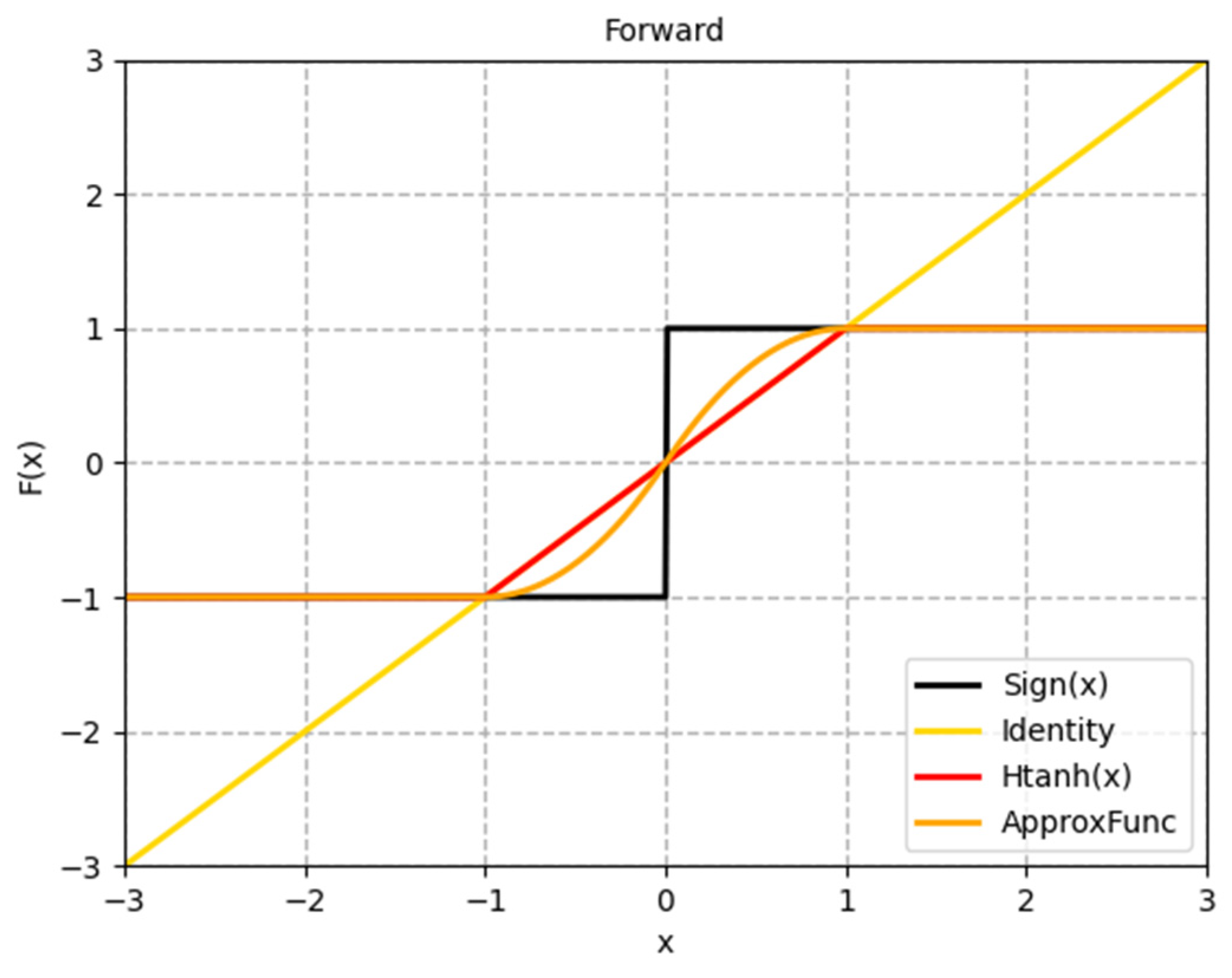
Similar to training a full-precision neural network model, a gradient descent-based backpropagation algorithm is used to update the parameters when training the binarized model. The binarized weights and activation values are used in the forward propagation process, and the full-precision parameters are updated in the backpropagation so that the model is fully trained. However, the derivative value of the sign function is almost always 0, which can lead to the disappearance of the gradient and the parameters cannot be updated for training purposes; thus, the gradient approximation is inevitably needed in backpropagation. In this study, three common approximation methods are used (Figure 3).
The first one uses the identity function (i.e., y = x ) to directly transfer the gradient information of the output value to the input value, completely ignoring the effect of binarization, which leads to a large gradient error due to the obvious gradient mismatch between the actual gradient of sign and the constant function; moreover, it accumulates errors during the backpropagation process, because of which the network training deviates from the normal extreme value point, resulting in an under-optimized binary network and, thus, seriously mitigating the performance.
The second method is a technique called the straight-through estimator (STE), proposed by Hinton et al. The STE is defined using Equation (5):
y = c l i p ( x , 1 , 1 ) = max ( 1 , min ( 1 , x ) )
The STE considers the effect of binary quantization on the part of cropping greater than 1 to reduce the gradient error. However, the STE can only pass the gradient information within the interval [−1, +1], and beyond that range, the gradient becomes 0. That is, once the value is outside the interval range [−1, +1], it can no longer be updated, and a problem similar to the death of neurons in the ReLu (Rectified Linear Unit) activation function occurs.
The third method is the ApproxSign function. Liu et al. proposed it in Bi-RealNet. The ApproxSign function replaces the sign function for gradient calculation in backpropagation, and it is expressed using Equation (6):
y = { 2 x x 2 , i f   0 x 1 2 x + x 2 , i f   1 x < 0 1 , o t h e r w i s e
The gradient approximates the gradient of the sign function in the form of a triangular wave, which is more similar to the impulse function than the STE, and thus more closely approximates the calculation of the gradient of the sign function. However, there is still the problem that the parameters are no longer updated once the values are outside the [−1, +1] interval.
However, it is crucial to ensure that all parameters are updated effectively during the model training process, especially at the beginning of the training.
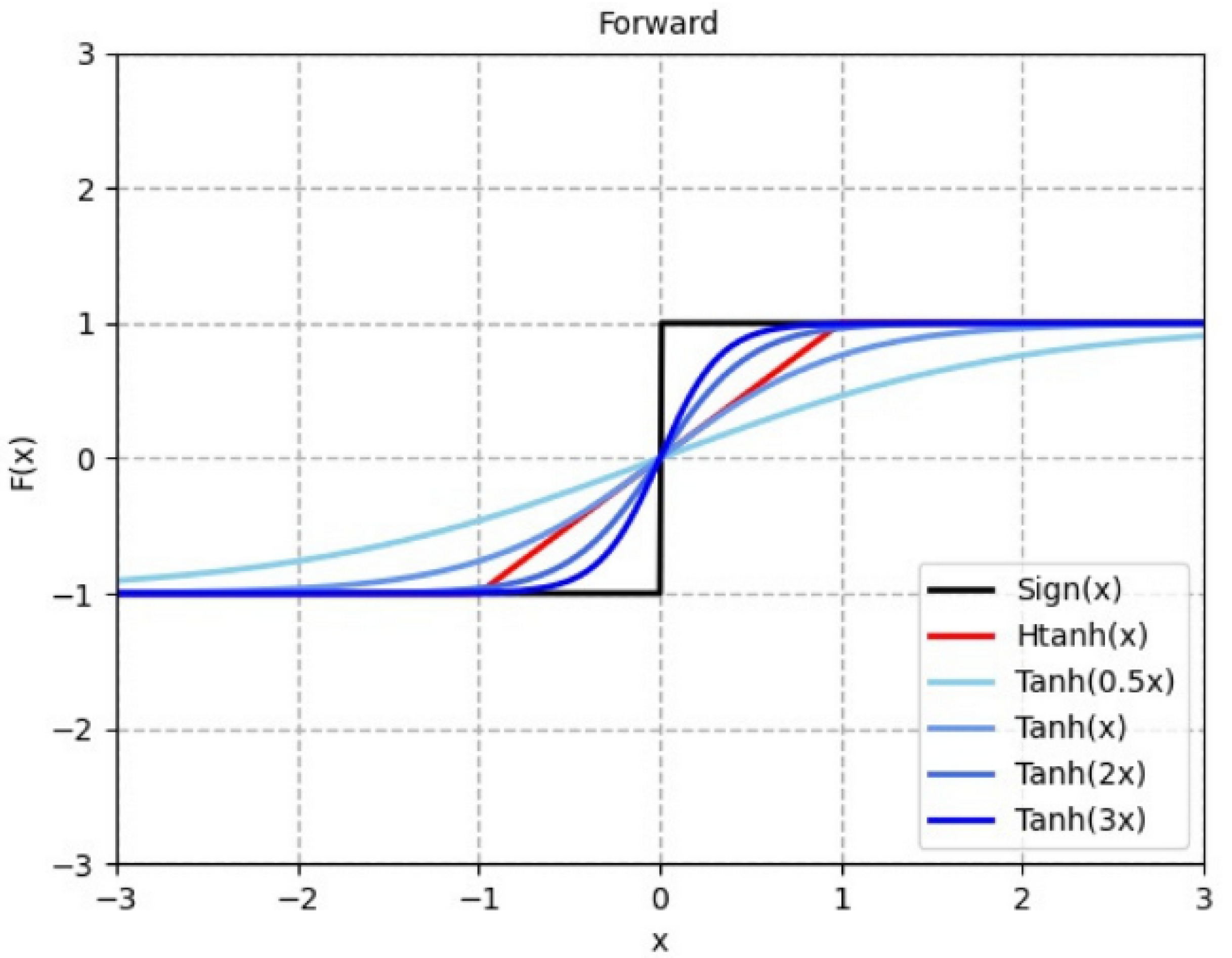
To address this problem, we propose an incremental training method, i.e., we try to ensure that all parameters are updated at the beginning of the model training. For this, the gradient of the backpropagation of the sign function is gradually approximated in the following training process. Instead of the sign for backpropagation, we design a function expressed using Equation (7):
y = tanh ( λ x )
where λ changes with the epoch during training expressed using Equation (8); k is a given using Equation (9):
λ = 2 k
k = k min + ( k max k min ) i N
where i is the number of epochs of the current training, N is the total number of epochs trained, k min set to −1 and k max set to 2. Our approximation function can effectively train parameters outside the interval [−1, +1]. As the training goes on, it is closer to the sign function than other approximate functions (Figure 4).

4. Experiments and Analysis of Results

To verify the effectiveness of the proposed method, in this section, we first present experiments conducted on the improved residual blocks using the cifar10 dataset. Then, extensive comparison experiments are conducted on the BIT-Vehicle public dataset, and ablation experiments are performed on the three proposed improvements.

4.1. Experimental Data Set and Experimental Parameters

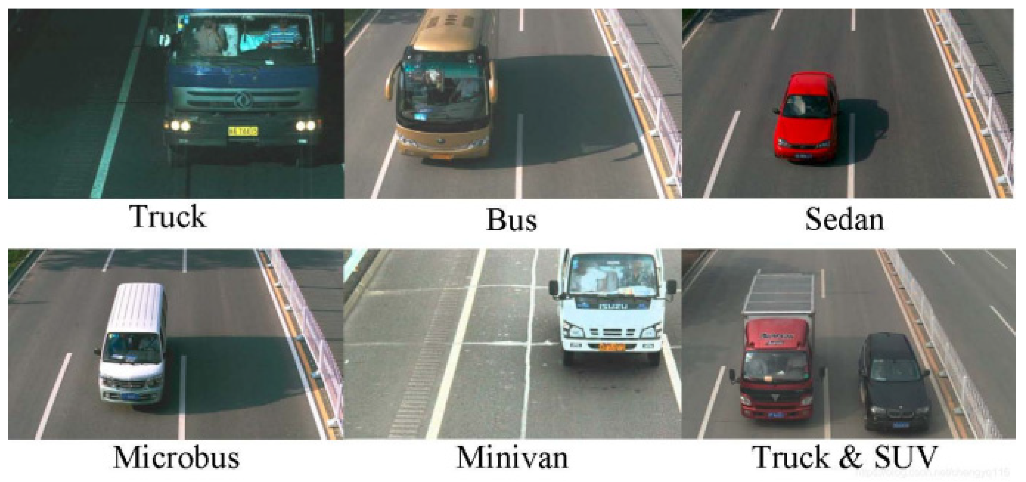
The BIT-Vehicles dataset was collected and organized by the laboratory of Beijing Institute of Technology. All images were intercepted from the actual road surveillance videos, and an example from the dataset is shown in Figure 5. The BIT-Vehicle dataset contains 9850 images (sizes of images may be 1600 × 1200 pixels or 1920 × 1080 pixels) of vehicles, which were captured using two cameras at different times and locations. In these images, there are variations in lighting conditions, scale, vehicle surface color, and perspective. Because of the capture delay and size of the vehicle, some top or bottom portions of the vehicle are not included. Two vehicles in the dataset appear in 203 images. After segmenting images containing multiple vehicles and separating the targets, there were 10,053 images, and the vehicles were classified into six categories; namely, bus, microbus, minivan, sedan, SUV, and truck, with 558, 883, 476, 5922, 1392, and 822 number of vehicles, respectively. The dataset was divided into a training set and a test set according to the ratio of 4:1.
This experiment was performed on a high-performance computer with a discrete graphics card, and a binary CNN was built using the Pytorch deep learning framework on an Ubuntu 16.04 operating system. The parameters of the development environment are shown in Table 1.
The parameters of the experimental training are set as follows: using the parameter update using an Adam optimizer, a weight reduction factor of 0.0001 was obtained, the Batchsize was set to 64, the initial learning rate was 0.001, and the learning rate was adjusted to 10% of the original when training 15, 30, and 40 epochs; a total of 50 epochs are trained.

4.2. Experimental Comparison and Analysis

We used Resnet18 as the benchmark model and binarized the network; except for the first convolutional layer and the fully connected layer, the rest of the layers were binarized with weights and activations. To improve the feature extraction ability of the binarization model for vehicle images from road surveillance viewpoints, a residual block adapted to the binarization network was designed, Abs-MaxPooling was proposed instead of traditional maximum pooling and average pooling, a weight redistribution binarization method was used in weight binarization, and a symbolic function gradient approximation and progressive training were used for training the binarized CNN. To ensure more an objective evaluation of the effectiveness of the proposed method, experimental results obtained using this method were compared with contemporary binarization models. Accuracy was used as the evaluation index; it was calculated by dividing the number of correctly predicted samples by the total number of samples.
To verify the advantages of the structure designed for the binarization model, the proposed binary residual block structure was analyzed with the number of parameters and the number of floating-point multiplication operations and compared with the number of heterogeneous or non-homogeneous operations in other studies (Table 2).
C i n , C o u t , W o u t , and H o u t indicate the number of input channels, number of output channels, output feature map width, and output feature map height of the downsampling layer, respectively. Our downsampling structure discards the number of floating points and floating-point multiplication operations, reducing storage-related overhead and improving model efficiency. To verify that our proposed structure works effectively, we experimented on the CIFAR-10 dataset using a binarized ResNet-20, and the experimental results are shown in Table 3.
Our structure can achieve the same accuracy as the contemporary best binarized networks, but it is more streamlined and has fewer parameters and operations, indicating that our residual block structure is accurate as well as fast.
We compared our method with various contemporary binarized CNNs and full-precision networks; the experimental results are shown in Table 4. The experimental results show that our method outperforms other binarized CNNs; the accuracy difference of full-precision networks is only 1.89%, which indicates that our method is effective.
To verify the effectiveness of Abs-MaxPooling, a comparison experiment was conducted using different pooling approaches as variables, and the experimental results are shown in Table 5. The positive and negative eigenvalues in the binarized CNN have equal contribution on the network. The maximum pooling focuses more on the positive features, while the average pooling distributes the gradient equally to all eigenvalues when the network is backpropagated; however, often, the eigenvalue with the largest absolute value in the pooling block affects the pooling results. Abs-MaxPooling solves the problems of the traditional pooling method in the binarized model and performs well in the binary CNN.

4.3. Ablation Experiments

To verify the effectiveness of the proposed methods, one of them is considered a control variable in the surveillance image dataset for ablation experiments, and the experimental results are shown in Table 6. All three proposed improvements bring gains to the binarized CNN.
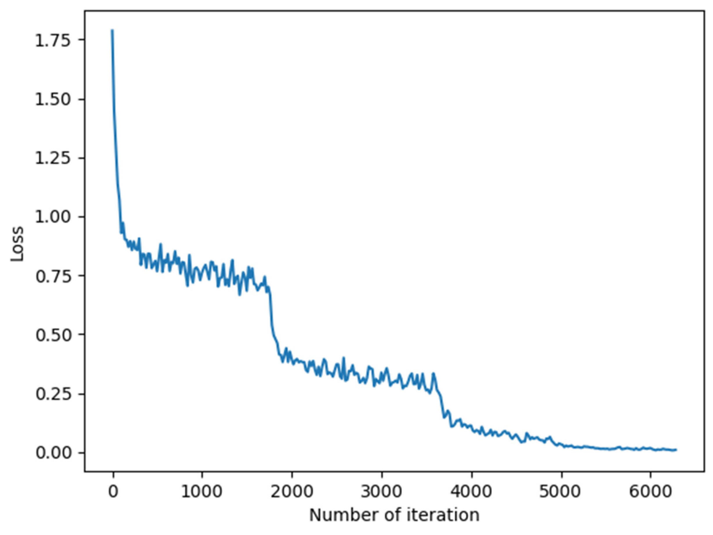
From the above experiments, we can see that both the improved binarization residual block and the weight redistribution binarization method can improve the classification accuracy of the binarization model. This is because in the binarized network, only a few parameters are outside the [−1, +1] interval after normalization, and the progressive training mainly plays a role in updating this part of the parameters. The training loss curve (Figure 6) and the test accuracy curve (Figure 7) are from the experimental result curves for Experiment 8.

5. Conclusions and Future Work

In this study, a binarized CNN-based vehicle classification method is proposed. First, the problems of full-precision CNN that inhibit direct binarization are addressed; to do this, the residual block adapted to the binarization model is redesigned, and Abs-MaxPooling is proposed. Then, the weights are binarized with weight redistribution, while discarding the additional floating-point gain terms, which reduces the number of floating-point parameters, and computation of the binarized network ensures the retention of the information of the binarized quantized weights and makes the training smoother. The progressive training method is used for training the binarization network so that the gradient is gradually closer to the symbolic function, which ensures that the parameters can be effectively updated during the training process while better matching the symbolic function gradient in the later stage of training. Experiments on the publicly available dataset CIFAR10 show that the proposed binary residual block structure leads to improved performance of the binarized CNN model. To verify the situation under real-time road conditions, further extensive experiments are conducted on the BIT-Vehicle dataset, and the results show that all the improvements demonstrate good results in the vehicle classification task under real-time surveillance.
Considering the limited distribution information representation capability of binarized networks, there is still a large gap between binarized models and full-precision models for more challenging tasks such as vehicle fine-grained classification and road surveillance vehicle detection. In future research, we will explore how binarized CNNs can be used to accomplish more complex tasks.

Author Contributions

Conceptualization, B.Z.; methodology, B.Z.; software, B.Z.; validation, B.Z.; formal analysis, K.Z.; investigation, K.Z.; resources, K.Z.; data curation, B.Z.; writing—original draft preparation, B.Z.; writing—review and editing, K.Z.; visualization, B.Z.; supervision, K.Z.; project administration, K.Z.; funding acquisition, K.Z. All authors have read and agreed to the published version of the manuscript.

Funding

This research was funded by the National Natural Science Foundation of China (No. 61971208), Yunnan Reserve Talents of Young and Middle-aged Academic and Technical Leaders (Shen Tao, 2018), Yunnan Young Top Talents of Ten Thousands Plan (Shen Tao, Zhu Yan, Yunren Social Development No. 2018 73), Major Science and Technology Projects in Yunnan Province (202002AB080001-8), Development and Application of Blockchain Service Platform Supporting Regional Integrated Energy Transactions Project of China (No. SGIT0000XTJS1900433), GHfund B (20220202, ghfund202202022131).

Data Availability Statement

Not applicable.

Acknowledgments

We thank our lab teachers and students for their support in the work of this paper.

Conflicts of Interest

The authors declare no conflict of interest.

References

  1. Simonyan, K.; Zisserman, A. Very deep convolutional networks for large-scale image recognition. arXiv 2014, arXiv:1409.1556. [Google Scholar]
  2. He, K.; Zhang, X.; Ren, S.; Sun, J. Deep residual learning for image recognition. In Proceedings of the IEEE Conference on Computer Vision and Pattern Recognition, Las Vegas, NV, USA, 26 June–1 July 2016; pp. 770–778. [Google Scholar]
  3. Courbariaux, M.; Bengio, Y. BinaryNet: Training Deep Neural Networks with Weights and Activations Constrained to +1 or −1. arXiv 2016, arXiv:1602.02830. [Google Scholar]
  4. Lin, X.; Zhao, C.; Pan, W. Towards accurate binary convolutional neural network. In Proceedings of the Advances in Neural Information Processing Systems, Long Beach, CA, USA, 4–7 December 2017. [Google Scholar]
  5. Tang, W.; Hua, G.; Wang, L. How to train a compact binary neural network with high accuracy? In Proceedings of the Thirty-First AAAI Conference on Artificial Intelligence, San Francisco, CA, USA, 4–9 February 2017. [Google Scholar]
  6. Darabi, S.; Belbahri, M.; Courbariaux, M.; Nia, V.P. BNN+: Improved binary network training. In Proceedings of the Sixth International Conference on Learning Representations, Vancouver, BC, Canada, 29 April–3 May 2018; pp. 1–10. [Google Scholar]
  7. Krizhevsky, A.; Hinton, G. Learning Multiple Layers of Features from Tiny Images; Technical Report TR-2009; University of Toronto: Toronto, ON, Canada, 2009. [Google Scholar]
  8. Dong, Z.; Wu, Y.; Pei, M.; Jia, Y. Vehicle type classification using a semisupervised convolutional neural network. IEEE Trans. Intell. Transp. Syst. 2015, 16, 2247–2256. [Google Scholar] [CrossRef]
  9. Rastegari, M.; Ordonez, V.; Redmon, J.; Farhadi, A. XNOR-Net: ImageNet classification using binary convolutional neural networks. In Proceedings of the European Conference on Computer Vision, Amsterdam, The Netherlands, 11–14 October 2016; pp. 525–542. [Google Scholar]
  10. Liu, Z.; Wu, B.; Luo, W.; Yang, X.; Liu, W.; Cheng, K.T. Bi-real Net: Enhancing the performance of 1-bit Cnns with improved representational capability and advanced training algorithm. In Proceedings of the European Conference on Computer Vision, Munich, Germany, 8–14 September 2018; pp. 722–737. [Google Scholar]
  11. Qin, H.; Gong, R.; Liu, X.; Shen, M.; Wei, Z.; Yu, F.; Song, J. Forward and backward information retention for accurate binary neural networks. In Proceedings of the IEEE Conference on Computer Vision and Pattern Recognition, Virtual. 14–19 June 2020; pp. 2250–2259. [Google Scholar]
  12. Liu, Z.; Shen, Z.; Savvides, M.; Cheng, K.T. ReActNet: Towards precise binary neural network with generalized activation functions. In Proceedings of the European Conference on Computer Vision, Virtual. 23–28 August 2020. [Google Scholar]
  13. Ding, R.; Liu, H.; Zhou, X. IE-Net: Information-Enhanced Binary Neural Networks for Accurate Classification. Electronics 2022, 11, 937. [Google Scholar] [CrossRef]
  14. Chen, P.Y.; Tang, C.H.; Chen, W.; Yu, H.-L. Dual path binary neural network. In Proceedings of the International SoC Design Conference (ISOCC), Jeju, Korea, 6–9 October 2019; pp. 251–252. [Google Scholar]
  15. Wang, P.; Cheng, Y.; Dong, B.; Gui, G. Binary Neural Networks for Wireless Interference Identification. IEEE Wirel. Commun. Lett. 2021, 11, 23–27. [Google Scholar] [CrossRef]
  16. Qian, Y.; Xiang, X. Binary neural networks for speech recognition. Front. Inf. Technol. Electron. Eng. 2019, 20, 701–715. [Google Scholar] [CrossRef]
  17. Jing, W.; Zhang, X.; Wang, J.; Di, D.; Chen, G.; Song, H. Binary Neural Network for Multispectral Image Classification. IEEE Geosci. Remote Sens. Lett. 2022, 19, 1–5. [Google Scholar] [CrossRef]
  18. Hasan, M.M.; Wang, Z.; Hussain, M.A.I.; Fatima, K. Bangladeshi Native Vehicle Classification Based on Transfer Learning with Deep Convolutional Neural Network. Sensors 2021, 21, 7545. [Google Scholar] [CrossRef] [PubMed]
  19. Habib, S.; Khan, N.F. An Optimized Approach to Vehicle-Type Classification Using a Convolutional Neural Network. CMC-Comput. Mater. Contin. 2021, 69, 3321–3335. [Google Scholar] [CrossRef]
  20. Chen, W.; Sun, Q.; Wang, J.; Dong, J.-J.; Xu, C. A novel model based on AdaBoost and deep CNN for vehicle classification. IEEE Access 2018, 6, 60445–60455. [Google Scholar] [CrossRef]
  21. Szegedy, C.; Liu, W.; Jia, Y.; Sermanet, P.; Reed, S.; Anguelov, D.; Erhan, D.; Vanhoucke, V.; Rabinovich, A. Going deeper with convolutions. In Proceedings of the IEEE Conference on Computer Vision and Pattern Recognition, Boston, MA, USA, 7–12 June 2015; pp. 1–9. [Google Scholar]
  22. Gong, R.; Liu, X.; Jiang, S.; Li, T.; Hu, P.; Lin, J.; Yu, F.; Yan, J. Differentiable soft quantization: Bridging full-precision and low-bit neural networks. In Proceedings of the IEEE International Conference on Computer Vision, Seoul, Korea, 27 October–2 November 2019; pp. 4852–4861. [Google Scholar]
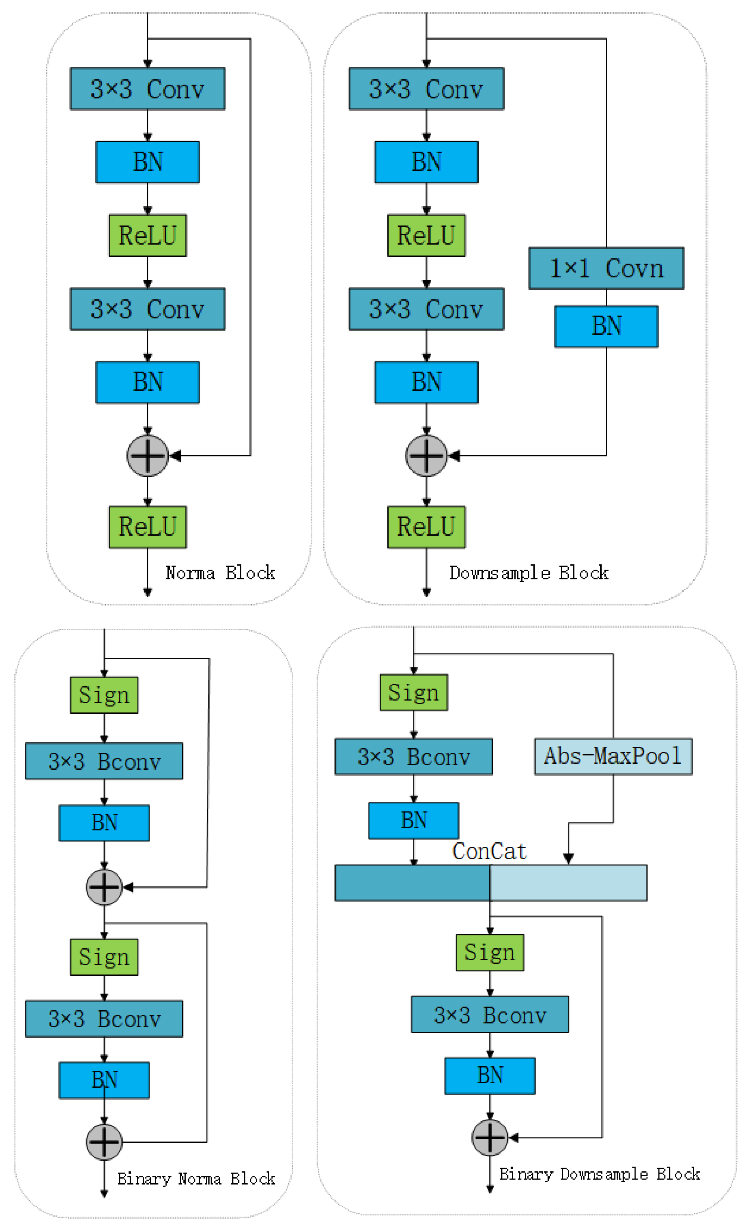
Figure 1. ResNet residual block and improved binarized residual block.
Electronics 11 01852 g001
Figure 2. Abs-MaxPool.
Electronics 11 01852 g002
Figure 3. Common approximation of a sign function.
Electronics 11 01852 g003
Figure 4. Hyperbolic tangent functions with different λ values approximated and compared with sign functions.
Electronics 11 01852 g004
Figure 5. Example of BIT-Vehicles dataset.
Electronics 11 01852 g005
Figure 6. Loss of binarization model experiment.
Electronics 11 01852 g006
Figure 7. Accuracy of binarization model experiment.
Electronics 11 01852 g007
Table 1. Experimental environmental parameters.
ItemParameter
CPUIntel Core i5-9400F 2.9 GHz x6
GPUNVIDIA GeForce RTX 2060
Operating systemUbuntu 16.04 LTS
Memory16 GB
Deep learning framework versionPytorch 1.7.1
Development languagesPython 3.6
Table 2. Comparison of number of parameters and calculation values of different descending sampling layers.
Downsampling ModeNumber of ParticipantsFloating-Point Multiplication Operands in ConvolutionXNOR Operands in Convolution
32 bit1 bit
ResNet 10 C i n C o u t + 2 C o u t 0 10 W o u t H o u t C o u t 0
Bi-Real-Net C i n C o u t + 2 C o u t 9 C i n C o u t W o u t H o u t C o u t 9 W o u t H o u t C o u t
Ours0 9 C i n C o u t 0 9 W o u t H o u t C o u t
Table 3. Accuracy of binarized ResNet-20 was evaluated using the CIFAR-10 data set.
ModelDatasetBinary ModelWeight/Activation (bit)Accuracy (%)
ResNet-20CIFAR-10Full Precision32/3291.2
DSQ [22]1/184.1
IR-Net1/186.8
ReActNet1/185.8
Ours1/186.3
Table 4. Comparison with classical binarization model.
DatasetBinary ModelModel Size (Mb)Weight/Activation (bit)Accuracy (%)
BIT-VehiclesFull-Precision (ResNet-18)42.6532/3296.66
BNN2.431/176.19
Bi-RealNet-189.201/189.60
XNOR-Net2.471/182.07
IR-Net (ResNet-18)2.051/192.33
Our model (ResNet-18)1.291/194.77
Table 5. Effects of using different pooling methods.
Pooling MethodAccuracy (%)
AvgPooling93.92
MaxPooling93.84
Abs-MaxPooling94.77
Table 6. Comparison of ablation experiment Settings and corresponding accuracy.
Experiment NumberBinarized Residual BlockBinarization of Weight RedistributionDynamic Progressive TrainingAccuracy (%)
1 82.51
2 90.84
3 92.64
4 84.27
5 93.91
6 93.89
7 91.85
894.77
Publisher’s Note: MDPI stays neutral with regard to jurisdictional claims in published maps and institutional affiliations.