PABAFT: Channel Prediction Approach Based on Autoregression and Flexible TDD for 5G Systems

Abstract

To achieve high gains from multiple antennas in 5G systems, the base station (gNB) constructs precoders using channel measurements obtained based on pilot signals. For high user mobility, the measurements quickly become outdated, which is especially crucial for ultra-reliable low latency communications (URLLC) traffic because it increases channel resource consumption to provide highly reliable transmissions and, consequently, reduces system capacity. Frequent pilot transmissions can provide accurate channel estimation and high-quality precoder but lead to huge overhead. Fortunately, 5G systems enable flexible time division duplex (TDD), which allows the gNB to dynamically change the configuration of downlink and uplink slots and tune the period of channel measurements. The paper exploits this feature and designs a new prediction approach based on autoregression and flexible TDD (PABAFT) that forecasts the channel between consequent pilots transmissions. To learn fine-grained channel properties, the gNB configures uplink pilot transmission in each slot. When the training data are collected, and the model is fitted, the gNB switches back to the regular slot configuration with a long pilot transmission period. Extensive simulations with NS-3 in high-mobility scenarios show that PABAFT provides the signal-to-noise ratio (SNR) close to that with the ideal knowledge of the channel at the gNB. In addition, PABAFT significantly reduces channel resource consumption and, thus, increases capacity for URLLC traffic in comparison to the existing solutions.

1. Introduction

The massive multiple-input multiple-output (MIMO) technology is a key part of 5G systems, promising significant improvements in network capabilities. However, the benefits and advantages of this technology rely heavily on the base station’s (gNB) ability to choose an efficient precoder. The precoder is a specific matrix that determines how the signals are transformed before the transmission from each antenna. So, the precoder is crucial in achieving the gains in throughput, capacity, and wireless system coverage.

In 5G systems, two approaches can be used to obtain downlink (DL) channel state information (CSI) for each user equipment (UE). With the first approach, the gNB sends special CSI reference signals (CSI-RSs). Each UE uses these signals to measure the channel and then sends the CSI report back to the gNB. The second approach is based on channel reciprocity, i.e., the effect that the DL channel properties are the same as for the uplink (UL) channel. The UE can send pilot signals called sounding reference signals (SRS), based on which the gNB measures UL CSI. If the channel is reciprocal, UL CSI coincides with DL CSI. Since the number of antennas at the gNB is much higher than at the UE, the second approach imposes a much lower overhead for pilot transmissions. Moreover, the second approach does not induce additional delay induced by sending the CSI reports from the UE to the gNB. That is why in 5G massive MIMO systems, the second approach is more widely used.

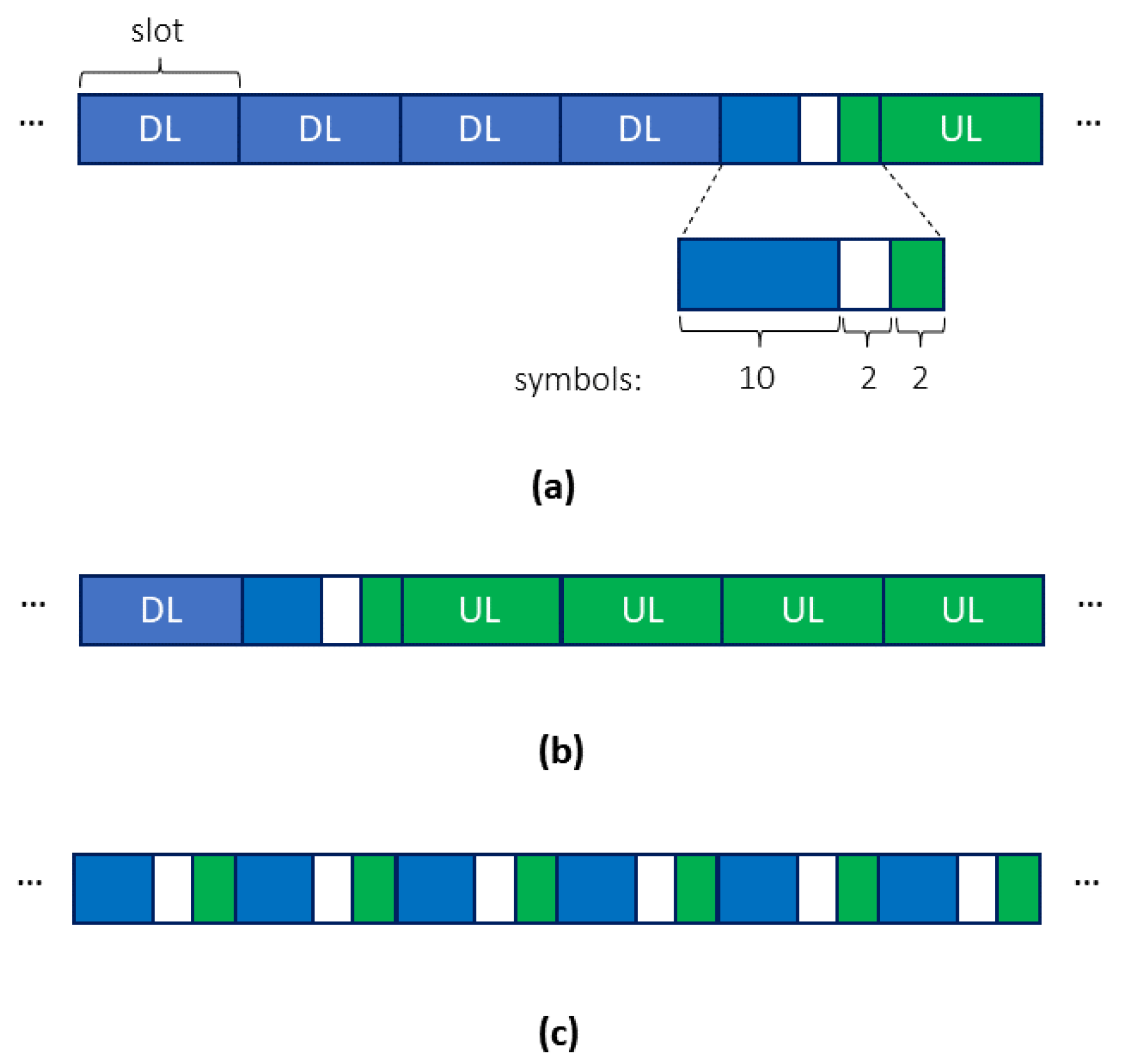
Channel reciprocity is only possible if the system uses time division duplex (TDD), according to which DL and UL transmissions occur in the same channel and are divided in the time domain. In contrast to 4G systems with quasi-static TDD, 5G enables flexible TDD, i.e., the order of DL and UL transmissions can be dynamically changed. Specifically, as illustrated in Figure 1, the time is divided into slots. Each slot consists of 14 orthogonal frequency-division multiplexing (OFDM) symbols. The gNB can allocate OFDM symbols of a slot to DL or UL transmission. To compensate the propagation delays, DL and UL transmissions shall be separated by several guard symbols. For example, Figure 1a shows that a slot contains ten DL symbols, two guard symbols, and two UL symbols.

Flexible TDD means that the gNB can dynamically configure the structure of each slot. Figure 1a shows an example of slot allocation for heavy DL traffic where most of the slots are allocated for DL transmission. UL slots/symbols can be used for data transmissions or SRS transmissions. Thus, by changing the TDD slot structure and allocating UL slots for SRS, the gNB can change the period of CSI measurements. As shown in Figure 1c, in theory, it is possible to make CSI measurements for each slot. However, this TDD structure imposes a huge overhead for guard and UL SRS symbols. Besides that, UL symbols need to be shared by several UEs.

UL CSI plays an important role in precoder selection and allows the gNB to adapt to the changing channel conditions. In the case of a single-user transmission, the gNB selects the precoder that maximizes the signal-to-noise ratio (SNR) at the UE based on UL CSI to improve the coverage and capacity of the cell. In rapidly changing environments, the gNB shall transmit CSI-RSs as often as possible because the channel changes quickly, and the channel state information becomes outdated. However, frequent channel measurements induce high overhead. Moreover, measurements are not possible in the slots allocated for DL transmissions. Thus, in high-mobility scenarios, the precoder obtained by previous UL CSI quickly becomes outdated, which significantly reduces cell throughput, as shown in many papers [1,2].

As shown in [3], a possible solution to this problem is a channel prediction algorithm that estimates the channel state in DL slots given previous CSI. With these predictions, it is possible to continuously adapt the precoder.

The core contribution of the paper is a new MIMO channel prediction approach called the prediction approach based on autoregression and flexible TDD (PABAFT). PABAFT extends the autoregression method in the following way. It uses frequent channel measurements in the training stage to fit a set of independent models for each intermittent slot between CSI measurements. Then it applies the fitted model to the rare measurements to predict the channel for data transmission. The main advantage of PABAFT is its ability to support ultra-reliable low-latency communications (URLLC) [4] in high-mobility scenarios. As we show with extensive simulations, the developed approach improves the coverage and decreases the channel resource consumption used for the URLLC traffic compared with the selection of state-of-the-art and baseline algorithms in multiple high mobility scenarios.

This paper is organized as follows. In Section 2, we briefly review the existing channel prediction approaches and explain why they are inapplicable for high-mobility scenarios and URLLC. We describe the PABAFT algorithm in Section 3. Section 4 discusses the performance evaluation results. Section 5 concludes this work.

2. Literature Review

Several classes of MIMO compatible channel prediction algorithms are considered in the literature, as summarized in

Table 1. Related works on channel prediction.

Method Class	Scenario	Prediction Target	Example Papers	Computational Cost	Training Data
Channel decomposition as SumOfSinusoids	WiMAX, Generic MIMO	CSI	[5,6,7,8]	Medium	Medium
Extrapolation	Generic MIMO	CSI	[9]	Low	None
Moving Average	5G URLLC	CQI values	[10]	Low	None
Geodesic precoding	5G	CSI	[11]	Low	None
Neural networks of various architectures	5G, LTE	CSI, CQI	[12,13,14,15,16,17,18,19]	High/Medium	High
Temporal Autoregressive Model (AR)	Generic Fading channel, LTE, 5G	CSI, CQI	[20,21,22]	Low	Low
Spatio-Temporal AR	5G	CSI	[19,23,24]	Low/Medium	Low/Medium

.

The first class includes such solutions as the estimation of signal parameters via rotational invariant techniques (ESPRIT) algorithm, its modifications [5,6,7] and Prony’s method [8]. These solutions rely on the channel decomposition: first, they estimate the parameters of the channel, such as delay spread and angle of paths; then, they extrapolate the channel state in the next moment from these channel parameters. The first step is generally computationally expensive, but the obtained channel parameters shall provide an accurate extrapolation for the future even in high mobility scenarios. Additionally, while channel decomposition approaches demonstrate high prediction accuracy for cases of very high antenna counts and bandwidths, the prediction accuracy is decreased when practical limits on bandwidth and antenna array sizes are introduced.

Another class consists of statistical algorithms that rely on collected channel state information to explicitly model the future channel properties as a function of previous measurements. This class includes linear extrapolation [9] and sliding window averaging [10]. Some papers, such as [11] model the channel state as a point on a certain manifold and extrapolate the channel by following a line on the created manifold from previous measurements. Recently, machine learning (ML) algorithms have been proposed, including those based on neural networks with different architectures [12,13,14,15,16,17,18,19]. Generally, the channel prediction task is formulated as a time series prediction problem. The authors use a variety of neural network architectures suitable for time series: recurrent neural networks for CSI prediction [12,13], convolutional neural networks [15], and combinations of both [14,16]. The paper [17], on the other hand, formulates the task as a reinforcement learning task, employing Q-learning for optimal beamforming.

While providing excellent results for the channel prediction problem, the neural networks face certain issues in practical deployment, namely, the high computational complexity of the algorithm. At the same time, they are required to be real-time. Additional problems arise from the need for a necessary training process with massive training sets, which are troublesome to gather. Moreover, adapting the trained model to a new channel environment is a challenging task, with multiple possible approaches, as evidenced in [18]. Finally, neural networks are less interpretable than other types of models. A possible solution to handle the massive data requirements for the training of the neural network is proposed in [12]. This paper studies a modified scheme of TDD, where the structure of the TDD frame itself is modified to minimize the overhead and supplement the channel estimation with a channel predictor based on a recurrent neural network. However, such an approach faces compatibility issues with the existing standard and legacy devices.

Therefore, these drawbacks drive the research towards both lightweight and high-accuracy methods. Possible candidates are autoregressive models (AR) [12,19,20,21,22,23,24], which provide high prediction quality along with low computational complexity.

The papers [20,21,22] study the dependence between the temporal AR model order and the performance of the resulting predictor, especially for long-range predictions and for high-velocity channels, which is an important consideration for predictor design. In [22] an AR model is used for channel quality prediction of the LTE-compatible satellite system.

In [19,23], an AR approach works in the spatio-temporal domain and uses the transformation from temporal to spatial (angle-delay) domain to accurately predict the channel in mobile scenarios. As the proposed predictors are working with angle-delay domain data, additional computational costs are incurred on top of fitting the model itself. Apart from that, with a low number of antennas, the accuracy of the approach decreases, which can limit the applicability of the approach to smaller MIMO arrays. The paper [24] tests the efficiency of Kalman filter-based and AR models in predicting the channel fading.

Since none of the described methods are designed to predict the channel with granularity higher than the frequency of the measurements during the inference phase while being compliant with the already existing network functions, in the paper, we design a new approach called PABAFT.

3. Description of PABAFT

PABAFT is based on the following model. The wireless channel between the gNB and the UE at the time instance t and the frequency f is represented as a complex matrix $H_f\left(t\right)$ of the size $N_{UE}\times N_{gNB}$, where $N_{gNB}$ and $N_{UE}$ are the numbers of antennas on the gNB and the UE, correspondingly. To simplify the description, we consider scenarios with a single antenna on the UE. However, the proposed approach can be easily extended to the case when $N_{UE}>1$.

According to 3GPP standards, the gNB operating in the channel of the bandwidth $BW$ divides the channel into narrow subbands called precoder groups (PGs). Within a PG, the channel is considered the same on various frequencies. Thus, when the gNB receives SRS, it averages measurements over all frequencies corresponding to a PG. Given an estimation of channel matrix ${\tilde{H}}_f\left(t\right)$ in PG f a time t, the gNB can construct the precoder matrix as follows:

$$P_f\left(t\right)=\frac{{\tilde{H}}_f^H\left(t\right)}{\left|\right|{\tilde{H}}_f\left(t\right)\left|\right|}\sqrt{Q},$$

where $H^H\left(t\right)$ is the Hermitian transpose and $\left|\right|{\tilde{H}}_f\left(t\right)\left|\right|$ is the Frobenius norm of ${\tilde{H}}_f\left(t\right)$, and Q is a power control diagonal matrix. This precoder is known as the maximum ratio precoder because it maximizes the SNR at the UE if the channel matrix is known accurately.

To predict the values of the elements of the matrix ${\tilde{H}}_f\left(t\right)$ at the next time moment, we propose to use the following approach. Let us consider the channel prediction problem as a time series regression problem where each matrix element is treated as a separate time series. The classical autoregressive model of order K predicts the value of the time series $y\left(t\right)$ based on K previous values as follows:

$$y\left(t\right)=c+\sum _{k=1}^K{\phi }_{k}y(t-k)+\epsilon \left(t\right),$$

(1)

where c is the constant bias of the model, ${\phi }_k$ is the autoregressive coefficient for each previous time step k, and $\epsilon \left(t\right)$ is the error term. For the classical autoregressive model, the time step equals the SRS period, i.e., the interval between two consecutive channel measurements.

In our approach, we modify the model as follows.

First, as the antennas are generally located close to each other in a certain array, small in comparison to the distance from the gNB to the UE, we use a single model for all elements of the matrix ${\tilde{H}}_f\left(t\right)$. Further, since the channel is similar in neighboring PGs, we use the same model (the same parameters) for F neighboring PGs. These assumptions allow us: (i) to reduce computational complexity and (ii) to reduce the time needed for training. Specifically, with F neighboring PGs, a single SRS gives us $F·N_{UE}·N_{gNB}$ samples to train the model. In Section 4, we analyze the validity of these assumptions and study the efficiency of the proposed approach depending on F.

Second, we take into account that the channel coefficients are complex-valued. The real and imaginary components of the complex numbers are considered independently, and a separate autoregressive model is applied to each component.

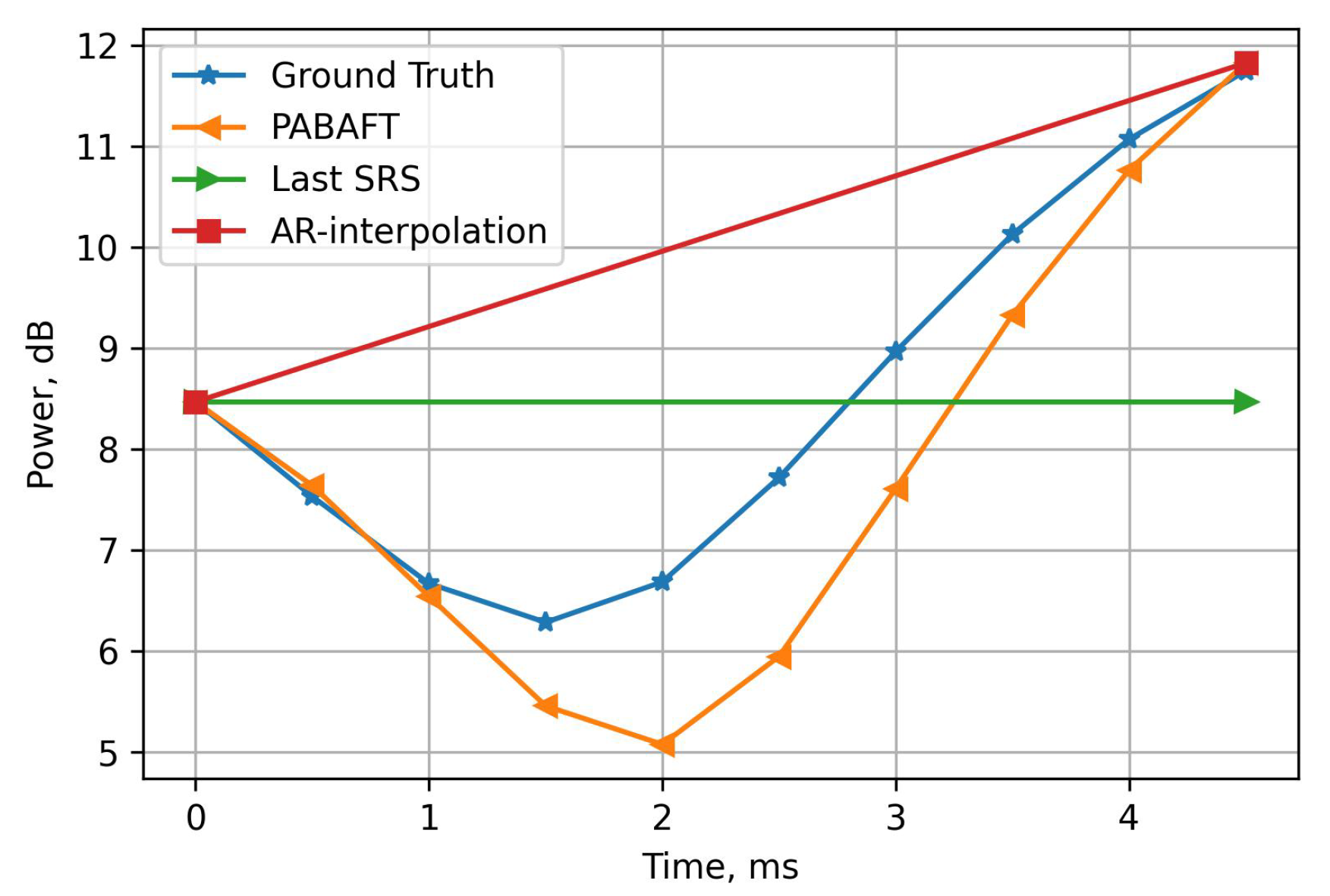
Third, the most crucial disadvantage of the standard autoregressive model (used in many related studies, see Table 1) is that the model uses discrete time, and to obtain a forecast for a moment between samples of the time series, it is necessary to use interpolation, which degrades the quality of prediction between the SRS measurements, especially if the CSI changes rapidly [21]. So, if the channel behavior between SRS periods is nonlinear, the error may be significant at the intermediate time instances even with an autoregressive model that predicts the channel state for the next SRS. One can observe this problem by comparing different channel prediction approaches during one SRS period of 5 ms, see Figure 2. Here, we show the estimated receive power from one transmitting antenna at one receiving antenna. We compare our approach (PABAFT), the usage of the last channel measurement (Last SRS), and the linear interpolation model with the ground truth. We can see that even though the linear model accurately predicts the channel for the next SRS period, it induces an error of about 8 dB in the middle of the SRS period. Thus, the linear model is only slightly better than the usage of Last SRS. Contrary to that, our approach can predict each slot with much greater accuracy.

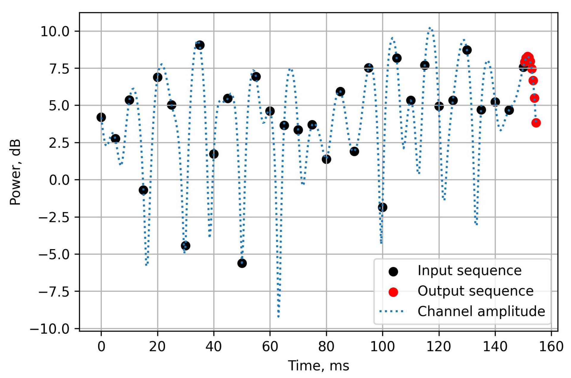
PABAFT uses the vector autoregression (AR) model as a predictor, where the target variables are the channel values at intermediate moments between the SRS transmissions and channel measurements using the SRS, while the coefficients for each variable are selected independently. PABAFT can be presented as a vector AR model, i.e., a set of independent linear models corresponding to different offsets within the SRS period. Here, such variables are the channel states in the output sequence seen in Figure 3. To train this model, we require a specific training phase that can span multiple frames, where we sample the channel in each uplink slot (which is possible due to Flexible TDD), allowing us to gather sufficient data to obtain a trained model for each downlink slot prediction in the inference phase, where downlink slots are prevalent. While the training phase does decrease the amount of resources that can be allocated to downlink data transmission, as shown in Section 4.2, the approach can reach high performance with a small number of training samples, meaning that the overhead on the training frames is insignificant.

The AR model is fitted using the standard Least Squares approach, where the training set was aggregated from all antenna pairs and multiple PGs. This approach improves the robustness of the model by introducing a more varied channel training set, as well as allows us to significantly decrease the number of frames necessary to achieve high accuracy of predictions.

4. Performance Evaluation

4.1. Simulation Setup

To compare the performance of PABAFT with other approaches, we use the NS-3 simulator [25] with the extended physical layer model. In particular, we use MIMO channel traces obtained with the QuaDRiGa channel model [26] that accurately follows the 3GPP channel modeling methodology [27]. The simulation parameters are summarized in

Table 2. Simulation Parameters.

Parameter	Value
Scenario	Urban Macro (UMa)
Carrier Frequency	3.6 GHz
Bandwidth	100 MHz (64 PG)
Channel state	Non-Line of Sight (NLOS)
UE speed	30, 60, 90 kmph
MIMO configuration	64 × 1
TDD frame size	10 slots
URLLC packet size	100 byte
URLLC packet period	10 ms
URLLC QoS requirements	10 ms delay budget, PLR $<{10}^{-5}$
SRS period	5 ms

.

We consider the Urban Macro (UMa) scenario with a gNB and a mobile UE moving at various speeds. The gNB is equipped with a dual-polarized $8\times 4$ rectangular antenna array (i.e., in total $N_{gNB}=64$ antennas). The UE has a single antenna ($N_{UE}=1$). The channel width is $BW=100$ MHz at 3.6 GHz, which corresponds to C-band widely used in 5G deployments. The OFDM numerology corresponds to 30 kHz subcarrier spacing. Consequently, a slot duration is 0.5 ms.

The TDD frame consists of $T=10$ slots. The configuration of DL/UL slots flexibly changes with time. During the training phase, the TDD is configured as shown in Figure 1c, and SRS is transmitted in each slot. Thus, the gNB obtains channel measurements with the granularity of a single slot. For L frames and F PGs, we obtain $S=L·F·N_{gNB}·N_{UE}$ samples that are used to train vector AR model, i.e., AR model for each of T slots in TDD cycle.

During the inference phase (working phase), the TDD structure is eight DL slots followed by two UL slots. SRS is transmitted in the last UL slot. Thus, the SRS period is 5 ms. As detailed in Section 3, each AR model uses K previous SRS measurements to predict the channel in a slot between the previous SRS and the next SRS, where K is called the model order. In our experiments, following the results from [5,20], we set $K=30$. We vary the number of samples S by changing L (i.e., by changing the duration of the training phase).

We compare the proposed channel prediction approach with the following approaches.

• Last SRS: the widely used approach according to which the gNB selects the precoder according to the last SRS measurement.
• Ideal: the gNB perfectly knows CSI. Therefore, this approach provides an upper bound on achievable SNR because no precoder aging is present in this approach.
• Geodesic: CSI for the intermediate slot is predicted according to the approach presented in [11].
• AR-interpolation: the CSI for the next SRS is predicted with the AR model (e.g., as in [12,19,20,21,22,23]), while the CSI in the intermediate slots is obtained based on interpolation.

We run two types of simulations. In the link-level simulations, we evaluate only the efficiency of the selected precoder. We consider a single PG and a fixed average pathloss between the gNB and the UE. We evaluate link level metrics, such as received power and SNR at the UE. In the system-level simulations, we model the whole stack from the application down to the physical layer. We consider a URLLC application that generates 100 bytes packets every 10 ms in DL. In the experiments, we measure the packet loss ratio (PLR) and the channel resource consumption.

4.2. Link-Level Simulation

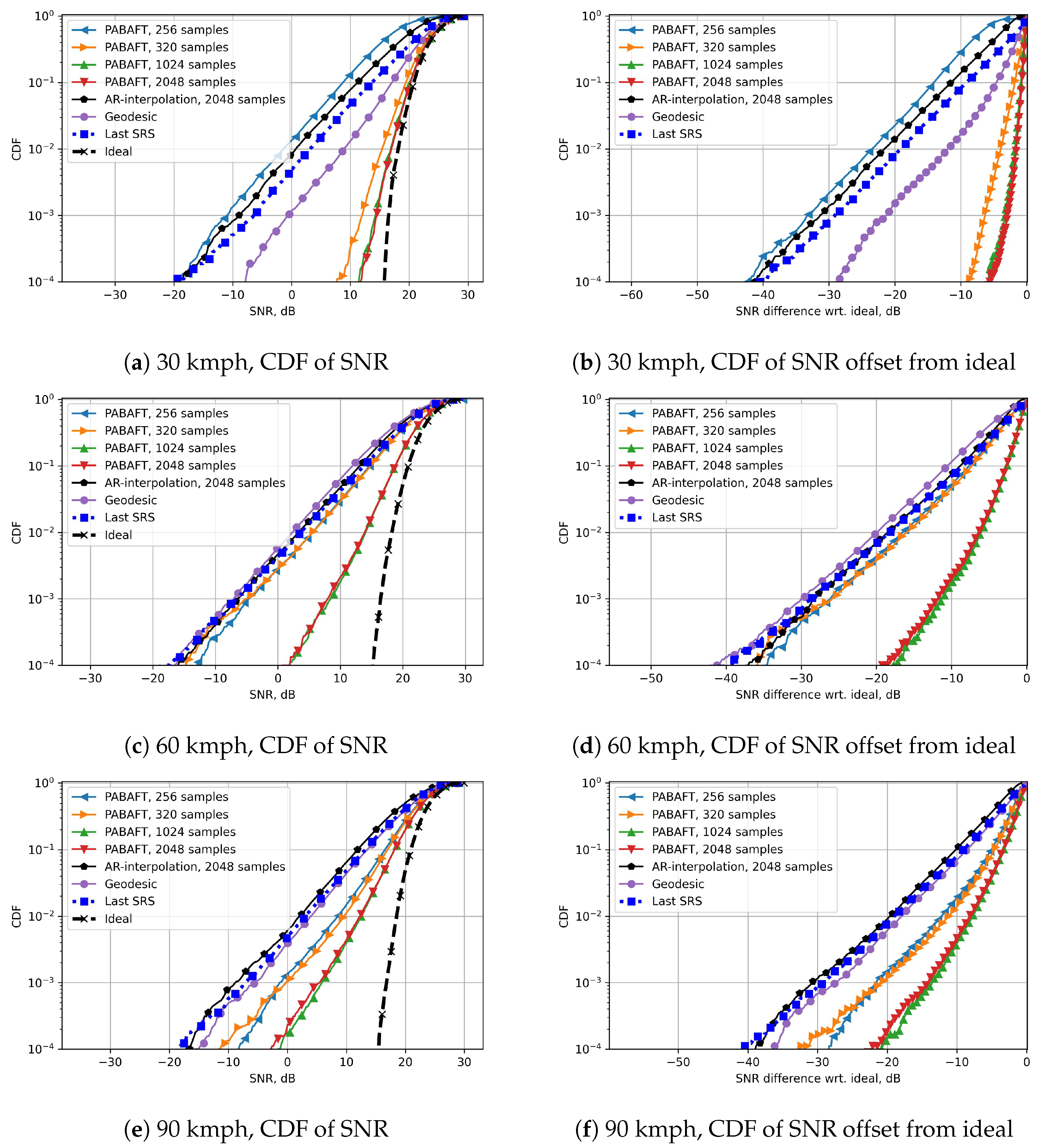
Figure 4 shows the link-level simulation results for a single PG (PG#1) and UE speeds of 30, 60, and 90 kmph. For each case, we plot two CDFs: (i) CDF of SNR at the UE, and (ii) CDF of the difference between SNR provided by a particular approach and SNR of the ideal channel prediction.

Let us consider the results for the 30 kmph case. The performance of the proposed PABAFT approach depends on the number of samples S used to train the vector AR model. For $S<300$, SNR is worse than for the Last SRS approach because the low number of samples is not enough to fit the model. A higher number of samples significantly improves the performance of PABAFT. Specifically, for $S>1000$, we can see that PABAFT provides SNRs close to the Ideal approach (the difference at the low quantile of ${10}^{-3}$ does not exceed 5 dB). Further increase of S does not improve the accuracy of the AR model and, consequently, PABAFT performance. Note that having $N_{gNB}=64$ antennas and a single PG, we need $L=16$ frames to train the model.

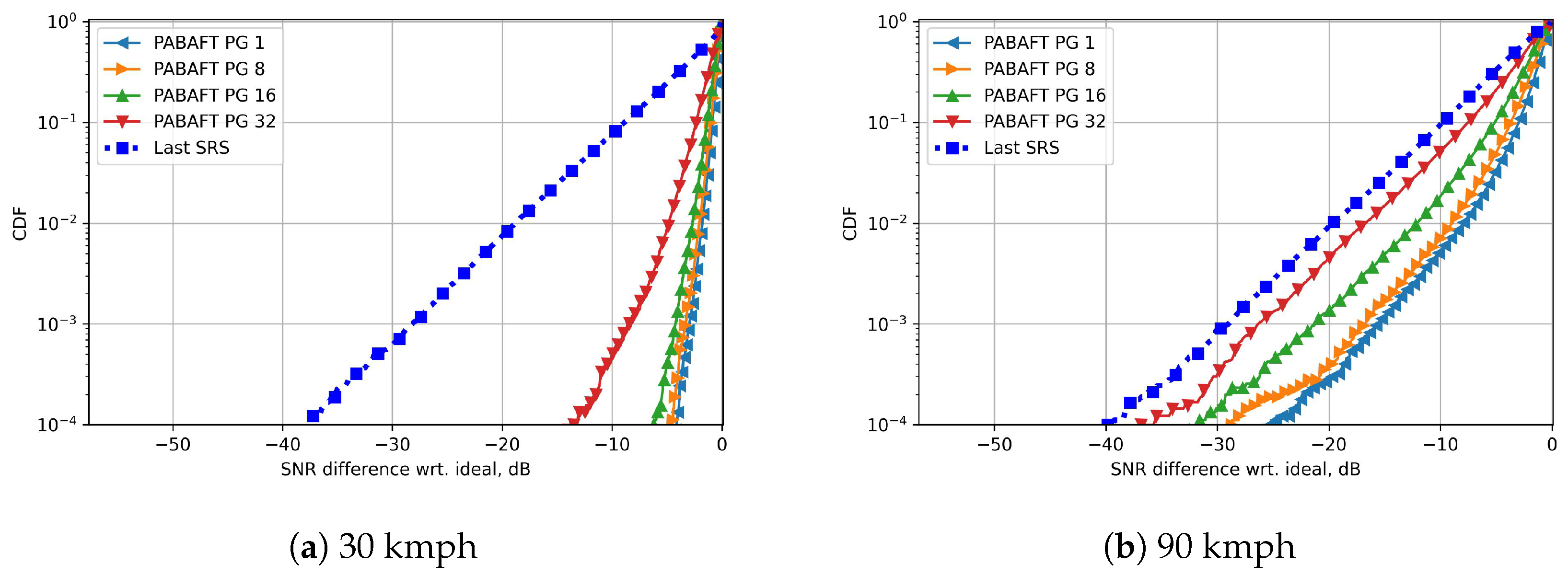
Let us study whether it is possible to aggregate measurements from different PGs to train the AR model. Figure 5 shows the results for the experiment in which the AR model is trained based on measurements from PG#1, and then the model is applied to predict the channel on PG#F. We can see that the CDF for PG number $F=8$ is close to the CDF for PG#1 (the difference is less than 1 dB). For $F\ge 16$ and high speed, we see significant degradation of performance. Thus, we can train a single AR model for a group of up to 8 PGs and aggregate measurements from different PGs to obtain more samples. For example, to obtain 1024 samples with $F=8$ PGs, we need $L=2$ frames, i.e., the training phase of only 10 ms is enough to fit the model. Further, in the system-level simulations, we aggregate $F=8$ PGs. For each group of 8 PGs, we train a separate AR model.

Considering other existing approaches presented in Figure 4, we can see that for 30 kmph speed, Geodesic provides approximately 10 dB improvement at ${10}^{-3}$ quantile with respect to Last SRS. However, the proposed PABAFT approach provides an additional 15 dB gain over Geodesic. Additionally, we observe that the AR-interpolation approach does not provide any significant improvement with respect to Last SRS because while it accurately predicts the channel for the slot when the next SRS is transmitted, the channel state for the intermediate slots is unknown and can be obtained only by interpolation. As illustrated in Figure 2, such interpolation induces significant channel prediction errors. In contrast, based on a short training phase, PABAFT constructs the AR model for each slot of a frame and much more accurately predicts the channel.

Let us consider the influence of UE speed on the performance of different approaches. From Figure 4c, we can see that the performance of Geodesic becomes even worse than Last SRS because of the increase in Doppler frequency from 100 Hz for 30 kmph to 200 Hz for 60 kmph, which is the channel sampling frequency for the SRS period of 5 ms. As the Geodesic approach extrapolates the channel state based on the two previous measurements, it cannot correctly predict the signal phase if the phase rotates more than $2\pi$ during one SRS period. The latter condition holds when the Doppler frequency exceeds the channel sampling frequency.

The performance of the PABAFT approach also degrades for higher UE speeds. However, even for 90 kmph, PABAFT still provides significant gain over other approaches: 15 dB gain at ${10}^{-3}$ quantile with respect to Last SRS and Geodesic. Note that 1024 training samples are enough to train the AR model irrespective of the UE speed. Thus, the duration of the training phase does not depend on the UE speed.

From the link-level simulation results, we can conclude that the proposed PABAFT approach: (i) provides a significant gain in SNR (more than 15 dB gain at ${10}^{-3}$ quantile) with respect to the existing approaches, (ii) requires a very low number of training samples that does not depend on the UE speed and can be measured during a single frame.

4.3. System-Level Simulation

In this section, we evaluate the performance of various channel prediction approaches for the case when the gNB transmits URLLC data in DL. The main peculiarity of the URLLC traffic is a very strict reliability requirement: the packet loss ratio (PLR), i.e., the ratio of packets not delivered within delay budget of 10 ms should not exceed ${10}^{-5}$. To provide such a low PLR, the gNB should select a robust enough modulation and coding scheme (MCS).

In our experiments, we configure the MCS selection algorithm at the gNB as follows. With the given TDD slot structure and delay budget, the gNB can make two transmission attempts of each packet. Thus, to provide PLR less than ${10}^{-5}$, the probability of erroneous packet transmission for a single attempt should be less than ${10}^{-2.5}$. To avoid boundary effects, we set target error probability $p={10}^{-3}$. For a given SNR estimation, the gNB can determine the MCS that provides an error probability below p. However, since SNR can change with time due to channel variation and precoder aging effect, the gNB selects MCS taking into account p-th quantile of SNR distribution [10]. Note that the higher is the obtained SNR quantile, the higher is selected MCS and, thus, the lower is the channel resource consumption for packet transmission.

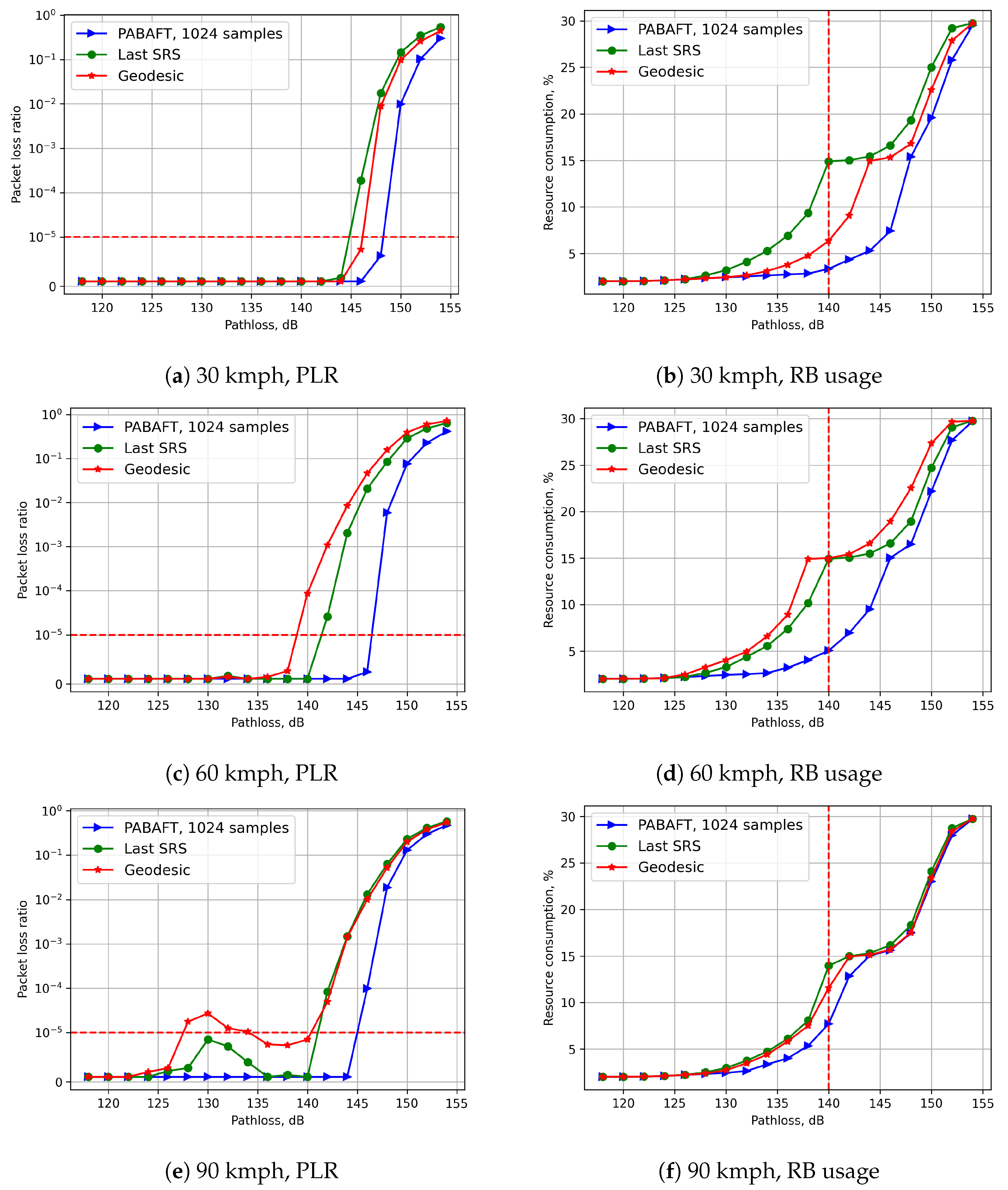
In Figure 6, we plot PLR and resource consumption as the functions of the average pathloss between the gNB and the UE. The intersection of the PLR curve with the horizontal line at ${10}^{-5}$ shows the coverage, i.e., the maximum pathloss at which the PLR requirement is satisfied. For 30 kmph, PABAFT provides up to 4 dB coverage improvement with respect to Last SRS and up to 2 dB improvement with respect to Geodesic. For higher UE speeds, the coverage for all the considered solutions reduces. However, the proposed PABAFT approach still provides up to 4 dB gain even at 90 kmph UE speed. Note that the performance of Geodesic is worse at 60 kmph speed than at 90 kmph speed. The explanation for this effect is similar to those mentioned in Section 4.2: Doppler frequency is close to the frequency of channel sampling leading to significant errors in the estimation of the signal phase.

Let us now compare the resource consumption of various approaches. For the pathloss of 140 dB and the UE speed of 30 kmph, the proposed PABAFT approach reduces the channel resource consumption up to five times with respect to Last SRS and up to two times with respect to Geodesic. This difference is explained by a significant improvement of p-th quantile of SNR obtained with PABAFT compared to the other approaches (see Figure 4a). With a higher SNR quantile provided by PABAFT, the gNB selects a higher MCS, reducing the channel resource consumption. Similar to the link-level simulation results, the increase in the UE speed raises channel resource consumption. However, even at 90 kmph, PABAFT provides over 60% reduction in the channel resource consumption compared with other approaches.

The obtained results show that the proposed channel prediction approach significantly improves the network performance serving URLLC traffic in terms of both coverage and channel resource consumption. Reducing channel resource consumption allows serving more UEs, i.e., increasing the network capacity.

5. Conclusions

In this paper, we developed a PABAFT approach for channel prediction based on a vector autoregressive model aided by the flexible TDD capabilities of 5G systems. Unlike other approaches based on machine learning with high computational cost, PABAFT can be implemented at the gNB with limited computational resources and uses only the standard specified network capabilities such as flexible TDD.

The developed approach splits the time into training frames, which are used to quickly estimate the channel variations, and then fit the vector autoregressive model, followed by inference frames, in which the fitted model predicts the channel with high accuracy. Alternation of train and inference frames allows PABAFT to consistently provide high accuracy predictions with a simple model in an online learning methodology.

Using simulations, we evaluated the efficiency of PBAFT in high-mobility scenarios. The link-level results show that the PABAFT is superior in terms of achievable SNR compared to other existing approaches. Specifically, PBAFT improves the ${10}^{-3}$ quintile of the SNR distribution up to 15 dB at 90 kmph UE speed that, in turn, allows for improving the performance of link adaptation algorithms for URLLC traffic. We have shown that it is possible to aggregate samples from neighboring frequencies to significantly reduce the duration of the training phase.

System-level simulation confirms that PABAFT improves coverage up to four dB and reduces channel resource consumption up to five times for a single URLLC flow. The latter means that PABAFT significantly increases the network capacity for URLLC traffic.

In our future work, we will consider the problem of adaptive selection of training/inference phase durations. The goal is to rarely run the training phase in order to reduce the overhead for measurements while providing a sufficient amount of training data to learn the vector autoregressive model.