Multiple Frequency Inputs and Context-Guided Attention Network for Stereo Disparity Estimation

Abstract

Deep learning-based methods have made remarkable progress for stereo matching in terms of accuracy. However, two issues still hinder producing a perfect disparity map: (1) blurred boundaries and the discontinuous disparity of a continuous region on disparity estimation maps, and (2) a lack of effective means to restore resolution precisely. In this paper, we propose to utilize multiple frequency inputs and an attention mechanism to construct the deep stereo matching model. Specifically, high-frequency and low-frequency information of the input image together with the RGB image are fed into a feature extraction network with 2D convolutions. It is conducive to produce a distinct boundary and continuous disparity of the smooth region on disparity maps. To regularize the 4D cost volume for disparity regression, we propose a 3D context-guided attention module for stacked hourglass networks, where high-level cost volumes as context guide low-level features to obtain high-resolution yet precise feature maps. The proposed approach achieves competitive performance on SceneFlow and KITTI 2015 datasets.

1. Introduction

Depth estimation is vital for extensive applications in practice, including augmented realities, autonomous driving and robotics, and it also could promote other computer vision task such as object detection and recognition. There are generally two manners to estimate the per-pixel depth of a scene, from a single monocular image or a pair of stereo images captured by a stereo camera. It is difficult for humans to infer the underlying 3D structure from a single image not to mention for computer vision algorithms, since a monocular image theoretically may correspond to numerous real-world scenes [1]. This paper aims to address the problem of depth estimation from stereo images, which computes the disparity map by the horizontal difference between the corresponding pixels on the left and right images. If an object at position $(x,y)$ in the left image is matched to position $(x-d,y)$ in the right image, the depth of the pixel position is then formulated as $\frac{fB}{d}$ [2], where f is the focal length of the camera and B is the distance between the camera centers.

The pipeline of traditional stereo-matching methods includes matching cost computation, cost aggregation, disparity regression and disparity refinement based on the local or global hand-crafted features [3]. Along with the development of deep learning methods, Convolution Neural Networks (CNN) are used to directly design end-to-end deep models [2,4,5,6,7,8] for depth estimation. Although such methods produce compelling disparity estimation results, two major issues remain challenging: predicting accurate result on boundaries and texture-less areas and precisely restoring the resolution of a disparity map.

Kendall et al. [5] proposed to firstly form 4D cost volume feature maps by concatenating left and right CNN feature maps across each disparity value, then employ 3D convolutions to filter the cost, and finally regress the disparity values with a differentiable soft-argmax operation. They trained the model end-to-end and obtained sub-pixel accuracy without additional post-processing or regularization. Chang et al. [2] further proposed the PSMNet method with stacked hourglass 3D CNN for processing the cost volume. Their framework has become the pipeline of deep stereo matching methods. 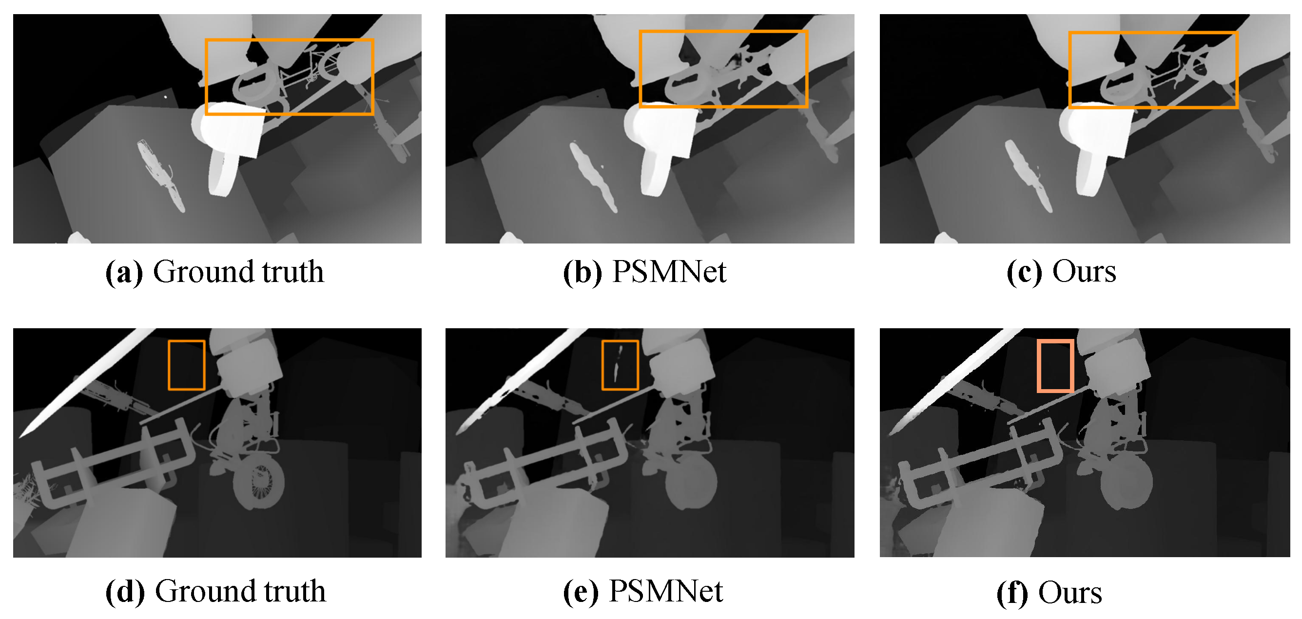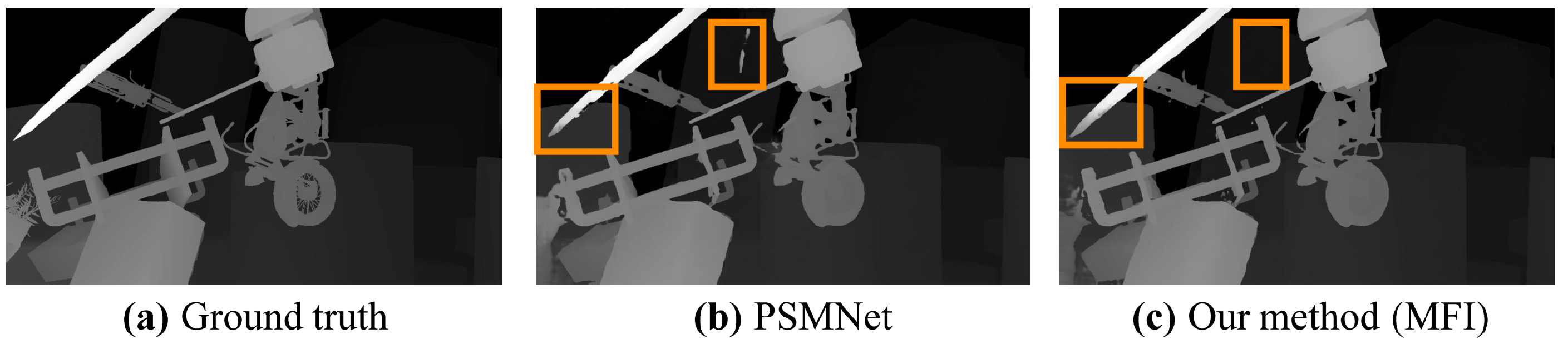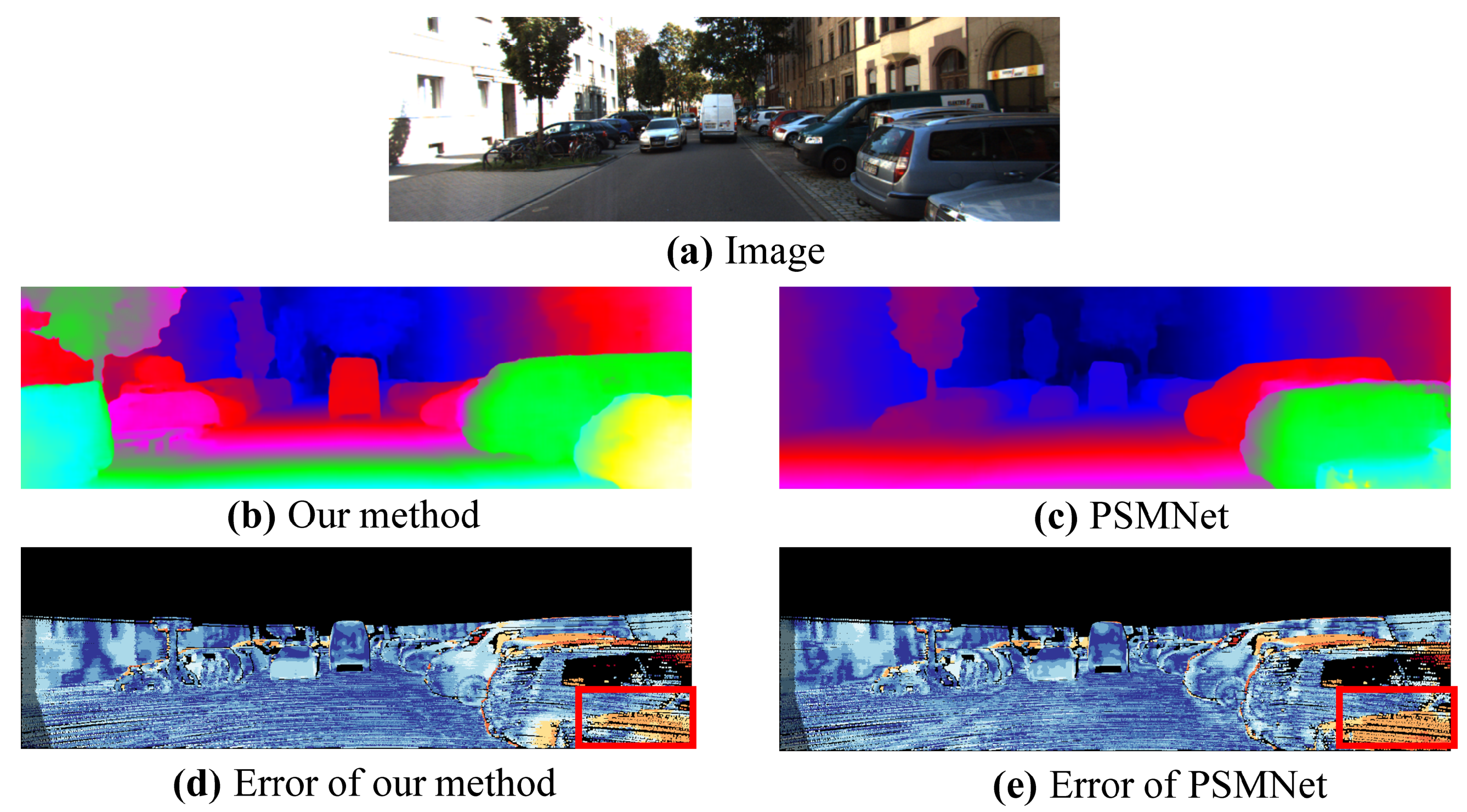Figure 1 shows the disparity maps obtained by PSMNet [2], from which we could see there are blurred boundaries and a deficient disparity continuity of the smooth region on the disparity maps. Many researchers have proposed methods to promote the disparity estimation by improving cost volume, such as forming the cost volume on area-based correlation [9], building multi-scale cost volumes [8] or packing a group-wise correlation map to form the cost volume [10]. All these methods learn feature representations from right and left RGB stereo images to form cost volumes by different ways. The corresponding information between right and left images may be lost at the feature learning stage, since the disparities are predicted improperly on boundaries and large texture-less areas. The research in the biology field [11] shows that when the spatial frequency information from the natural image enters the visual system through the retina, it might be dissected into three different frequency channels (low, medium and high components) in the superficial layer of the primary visual cortex. Inspired by them, we heuristically take multiple frequency inputs including a low-frequency component, RGB image and high-frequency component into CNN to extract abundant features for forming cost volume. In this way, the high-frequency component could emphasize the feature extraction on boundaries; meanwhile, the low-frequency component takes charge of texture-less smooth regions.

Following cost volume computation, learning-based methods also make use of a deep neural network to optimize the cost volume. High-level features which are learned to aggregate the cost volume with convolutions have lower resolution than original stereo images; in this case, they are weak in restructuring the original dense depth prediction precisely. Increasing the resolution operators, such as up-sampling, decoder and deconvolution, are consequently needed. A representative method [2] learned 3D CNN to regularize cost volume by stacked multiple hourglass networks (encoder–decoder) in a top–down/bottom–up manner for regional support of context information. Furthermore, a lot of research is conducted on cost optimization to improve stereo matching, such as introducing non-local attention module [4,9], utilizing a recurrent unit to update disparity estimations at high resolution [8], adding constraints to the cost volume with unimodal distribution peaked at true disparities [12], or introducing a patch attention block to aggregate disparity information on the different surfaces of cost volume [13]. Inspired by these methods and an up-sampling module in semantic segmentation [14], we extract the context information of high-level cost volume features to weight low-level high-resolution features by an attention mechanism in stacked multiple hourglass networks. In this way, context information of the disparity between left and right images could be more fully utilized to obtain depth details when recovering the resolution of a disparity map.

In summary, we propose two simple but effective improving strategies based on an end-to-end framework PSMNet [2] in this paper for stereo matching. Specifically, (1) we extract pixel-level high-frequency and low-frequency components named boundary and smooth maps, respectively, from stereo RGB images. Then, we feed them into a CNN model to feature extraction for cost volume computation. (2) To take advantage of context information in cost volume, we learn the relative importance of dense feature maps by the guidance of high-level features when processing cost volume to generate a dense disparity map. Our method is validated on SceneFlow and KITTI 2015 datasets. Experimental results show that the performance of our model with multiple frequency inputs and a context-guided attention strategy is better than that of the base network PSMNet [2], and our method obtains competitive results compared to related state-of-the-art methods.

Roadmap. In Section 2, we first introduce the related work. The proposed approach for depth estimation is described in Section 3. Experiments are shown in Section 4, and the conclusion is in Section 5.

2. Related Work

A stereo matching algorithm generally consists of matching cost computation, cost aggregation, disparity computation and refinement. The matching cost measures the dissimilarity of the corresponding pixels, super-pixels or patches between the left and right images, which could be computed with hand-crafted features or learned features.

Matching cost computation. CNN has been widely utilized for computing the matching cost leveraging the development of deep learning in recent years. Zbontar et al. [15] trained a deep Siamese network to compute the similarity between $9\times 9$ patches to form matching cost. Luo et al. [16] also proposed a Siamese network in which the computation of matching cost is treated as a multi-label classification problem. Post-processing steps, such as cost aggregation and smoothing, are still needed in these methods. Kendall et al. [5] proposed an end-to-end model GC-Net for stereo matching by forming 4D cost volume feature maps, processing the cost with 3D convolutions and regressing disparity values with soft-argmax operation. Chang et al. [2] proposed PSMNet to exploit global context information in stereo matching with a pyramid pooling module and stacked hourglass 3D CNN. These methods form the cost volume by concatenating left feature maps with their corresponding right feature maps across each disparity level, resulting in a 4D volume on height, width, disparity levels and the size of the feature map.

Recently, many researchers have proposed methods to promote the disparity estimation by improving cost volume. Li et al. [9] utilized the area-based correlation to capture more local similarity in cost volume; then, they combined an hourglass module with non-local attention as the 3D feature matching module (Abc-Net). Wang et al. [8] built multi-scale cost volumes and then adopted a recurrent unit to iteratively update disparity estimations at high resolution. Guo et al. [10] proposed GwcNet to split the deep features into multiple groups along the channel dimension to obtain group-wise correlation maps, which are packed to form a 4D cost volume. Shen et al. [17] proposed a fused cost volume representation to deal with the large domain difference and a cascade cost volume representation to alleviate the unbalanced disparity distribution. Daggal et al. [18] proposed the DeepPruner method by reducing the computation of cost volume to achieve real-time stereo matching. Xu et al. [19] presented a cost volume construction method by generating attention weight for cost volume with multi-level adaptive patch matching. Gu et al. [20] proposed to build cost volume upon a feature pyramid encoding geometry and context at gradually finer scales. All these deep methods employed three-channel RGB images to feed into CNN for learning the matching cost. Different from them, we input multiple frequency images to extract more features about boundaries and texture-less smooth regions for forming cost volume; thus, the disparities on these locations could be recovered more accurately.

Auxiliary cues. Auxiliary cues have been exploited into stereo matching to improve the accuracy of depth estimation. Ladicky et al. [21] jointly optimized stereo reconstruction and object segmentation by random field labeling. Guney et al. [22] utilized the object information of vehicles to resolve ambiguities in stereo matching. Yamaguchi et al. [23] proposed to jointly recover an image segmentation and a dense depth estimation, in which adjacent segments are encouraged to be similar if they belong to the same object. Menze et al. [24] applied adaptive smoothness constraints for a dense stereo estimation with a conditional random field. Yang et al. [25] proposed the SegStereo method by employing semantic features from segmentation for disparity estimation. Wang et al. [26] proposed to incorporate gradient-domain smoothness prior and occlusion reasoning into a stereo network to help the network generalize better. Rao et al. [27] proposed a multi-task learning architecture with visual attention mechanisms for semantic segmentation and disparity estimation. Zhang et al. [28] proposed a co-learning framework with monocular and stereo branches to improve stereo performance. Song et al. [29] proposed the EdgeStereo method, which is a multi-task learning network composed of a disparity estimation branch and an edge detection branch, in which the edge features are embedded into the disparity branch, providing fine-grained representations. Yang et al. [30] designed a separate processing branch edge stream in parallel with the stereo stream to learn geometric information. These methods utilized auxiliary information such as object, semantics, edge or smoothness for stereo matching. Compared to these methods [23,24,26] with smoothness constraints on a disparity map, our low-frequency input component could help the feature learning of texture-less regions for forming cost volume. Compared to [29,30], which estimates the disparity and edge simultaneously, we input the high-frequency edge information of the original image into a CNN model to assist feature learning.

Processing on cost volume. Chang et al. [2] designed a stacked hourglass 3D CNN to regularize the cost volume, in which encoder–decoder architecture was used to aggregate context information on cost volume for pixel disparity prediction. Zhang et al. [6] proposed GA-Net with cost aggregation layers for end-to-end stereo reconstruction to replace the use of 3D convolutions. Cheng et al. [31] proposed a convolutional spatial propagation network (CSPN) to learn the affinity matrix, and they used it in a 3D version to propagate information along the disparity value space and scale space. Zhang et al. [12] proposed to directly add constraints to the cost volume by filtering cost volume with unimodal distribution peaked at true disparities. Xu et al. [32] proposed AANet to approximate the cross-scale cost aggregation algorithm with neural network layers to handle large texture-less regions. Tosi et al. [7] proposed Stereo Mixture Density Networks (SMD-Nets) and formulated the stereo-matching task as a continuous estimation problem by bimodal mixture densities. Rao et al. [13] introduced patch attention network (PA-Net) with a channel-attention mechanism to aggregate disparity information on the different surfaces of cost volume. Rao et al. [4,33] designed a non-local context attention network (NLCA-Net) to exploit the global context information for regularizing the cost volume. These methods improve stereo matching in terms of cost optimization; among them, the most relevant work to our method is attention-based methods [4,13,33]. In their methods, attention-based feature learning on cost volume is carried out within the feature layer, while the cross layer attention mechanism is designed to process the 4D cost volume in our method; thus, more context information could be utilized to recover the disparity map.

Different from typical deep stereo matching methods and our proposed method, the most recent two methods do not build a full 4D cost volume. Tankovich et al. [34] proposed a multi-resolution initialization step to infer disparity hypotheses and a propagation stage to refine the disparity. Li et al. [35] proposed three stages of cascaded recurrent network to compute different scales of stereo correlation, and the former stage output disparity is fed to the next as an initialization to obtain a refined disparity iteratively.

3. Our Approach

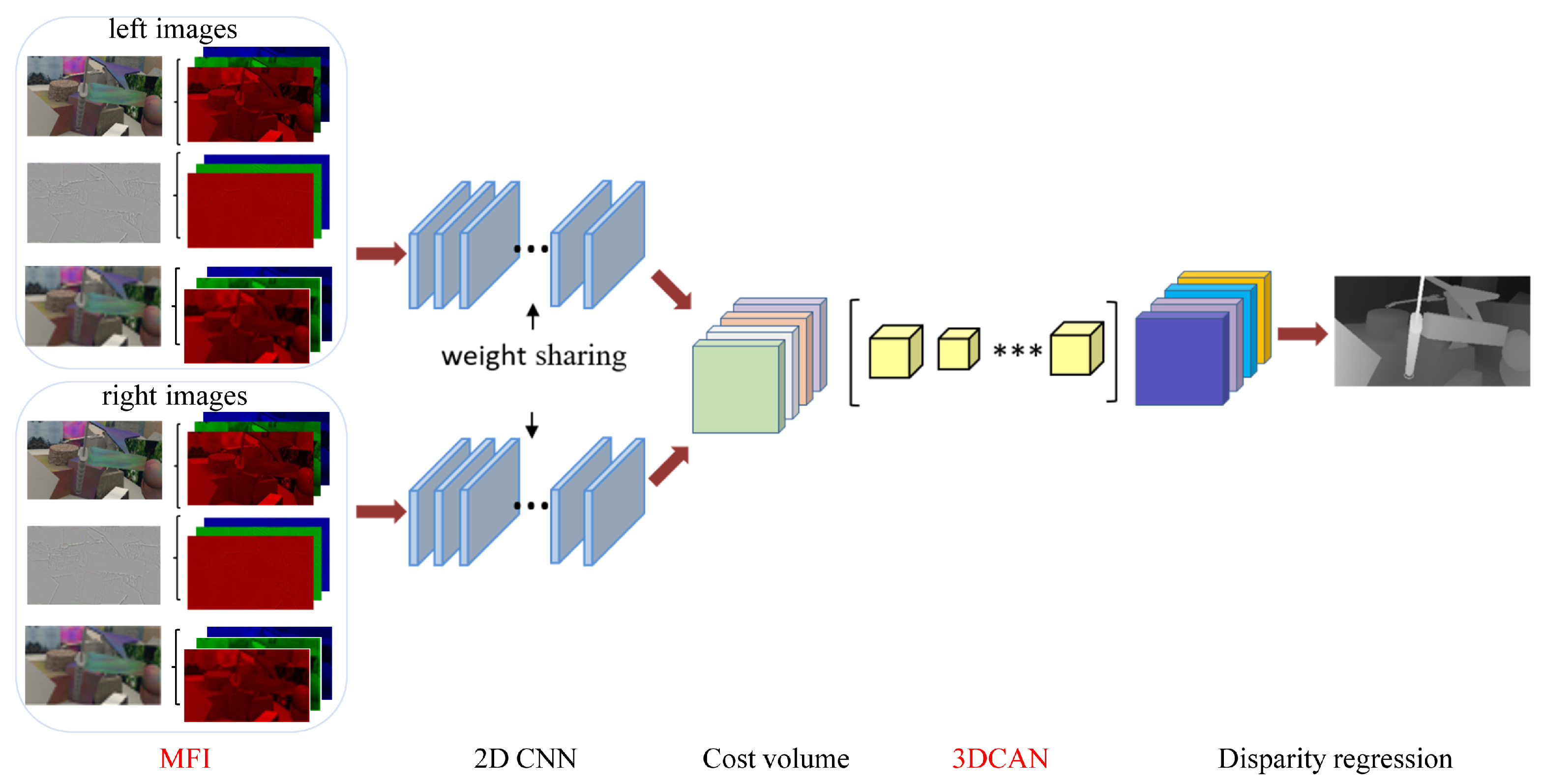
In this section, we describe the proposed multiple frequency input and context-guided attention network for stereo matching, and the whole architecture is shown in Figure 2. Our architecture consists of five main steps, obtaining multiple frequency inputs, 2D CNN for feature extraction, forming cost volume, attention-based cost volume regularization and disparity regression. The stereo image pairs and the corresponding high-frequency and low-frequency components are utilized as the Multiple Frequency Input (MFI) into the two weight-sharing 2D convolution networks to obtain feature maps. The produced feature maps from the right and left images are adopted to form a 4D (height × width × disparity levels × feature size) cost volume across each disparity level. Then, the cost volume is fed into our 3D Context-guided Attention Network (3DCAN)-based stacked hourglass architecture. The 3DCAN optimizes the matching cost computed from the feature maps. Finally, a softmax operation is performed on the matching cost, and the cost volume is converted into probability to perform disparity regression to obtain disparity estimation results. We briefly introduce 2D CNN; then, MFI, 3DCAN and the loss function are described in following sections.

Multiple frequency input is fed into 2D CNN, which has three layers of $3\times 3$ convolution filters, four basic residual blocks, and an SPP module [2]. SPP uses four average pooling blocks to compress the output of residual blocks into four scales, which are then, respectively, followed by $1\times 1$ convolution and up-sampling via bilinear interpolation to the same-sized feature maps. Then, the different levels of feature maps are concatenated as the output of 2D CNN.

3.1. Multiple Frequency Inputs

The input of convolutional neural network is generally an RGB three-channel image in all of the above-mentioned stereo matching methods, such as GC-Net [5] and PSMNet [2]. It is still a challenge issue to predict accurate disparities on boundaries and texture-less areas for existing methods, such as the estimation results by PSMNet [2] shown in Figure 1. From the figure, we could find that the disparities are inaccurate at the boundaries of the box marked objects in Figure 1b and the continuous region in (d). This is because the correspondences of these regions are provided by the neighbor pixels, which belong to other objects or background during the matching processing between right and left images. Therefore, it prompts us to design a stereo matching network that could specially learn the representations of boundaries and continuous regions on images. The research in the biology field [11] shows that when the spatial frequency information from natural images enters the visual system through retina, it might be dissected into three different frequency channels (low, medium and high components) in the superficial layer of the primary visual cortex. Inspired by this, we propose to firstly obtain the high-frequency and low-frequency components from an RGB image; then, we feed three of them together (multiple frequency) into a 2D CNN model. We suppose that the high-frequency component could emphasize the feature extraction on boundaries; meanwhile, the low-frequency component could emphasize the feature extraction for texture-less smooth regions.

In this paper, we refer to a nonlinear total variation algorithm [36] to obtain multiple frequency images. We assume image $I_{x,y}$ is composed of two parts, that is $I_{x,y}=B_{x,y}+S_{x,y}$, where x and y are coordinates. S is expected to be obtained from image I by the following function,

$$L\left(S_{x,y}\right)=\frac{1}{2}\sum _{x,y}{(S_{x,y}-I_{x,y})}^2+\lambda \sum _{x,y}\sqrt{{(S_{x+1,y}-S_{x,y})}^2+{(S_{x,y+1}-S_{x,y})}^2}$$

(1)

where $\lambda$ is the trade-off parameter. S is reconstructed from the original image by minimizing the above function. The first item aims to ensure S is similar to I; thus, S could preserve the effective information of the original image. The second item in the above function is the total variation norm, which could help obtain a smooth image S. With $B_{x,y}=I_{x,y}-S_{x,y}$, we obtain the oscillating regions of the image. 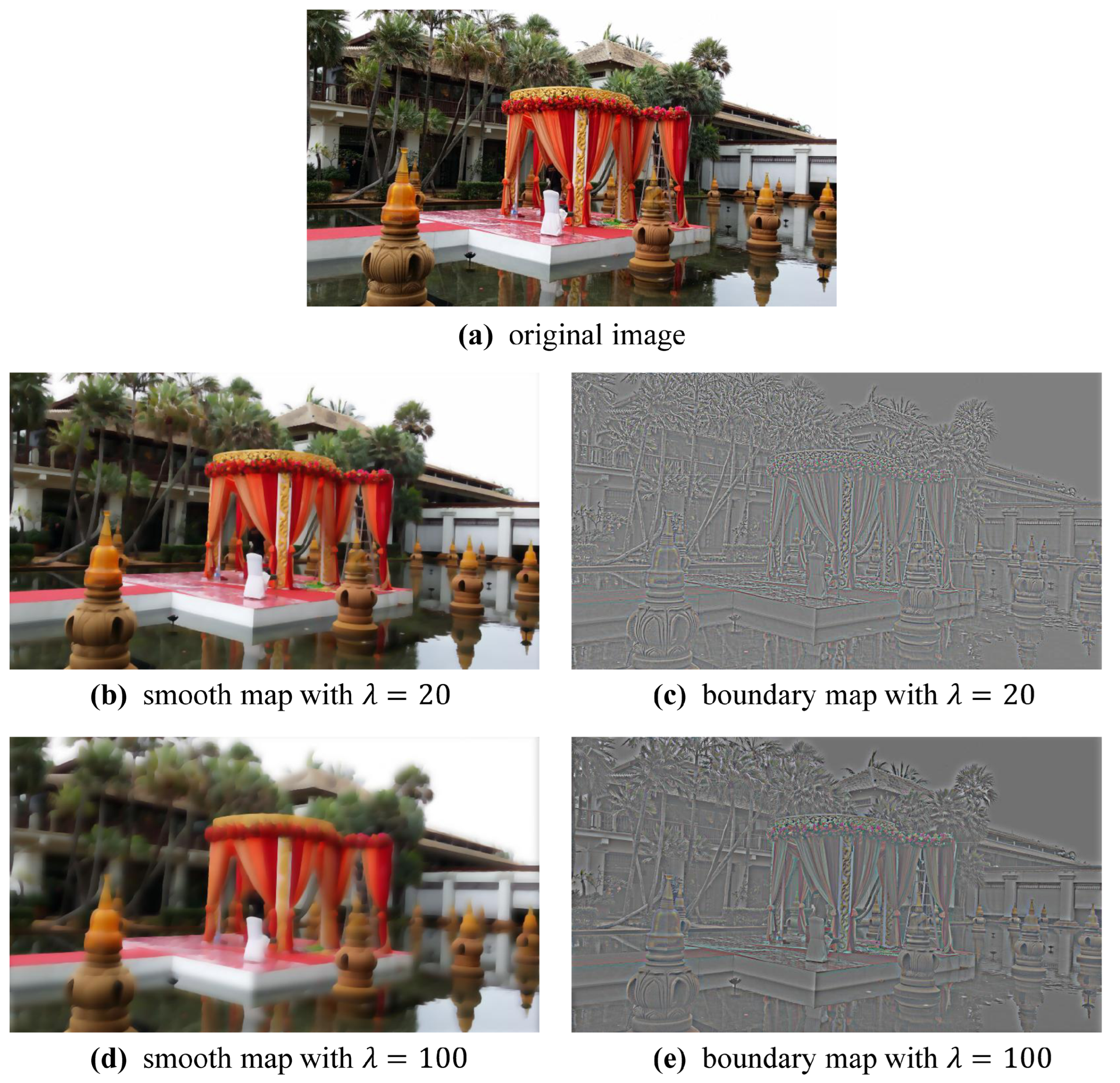We intuitively name S and B as the smooth map and boundary map, respectively. Note that the three-channel smooth and boundary maps are separately computed from RGB images. We adopt the gradient descent method to optimize the above function and obtain its local minimum. Smooth and boundary maps are illustrated in Figure 3 with a different trade-off parameter $\lambda$. It could be seen that the more blurred smooth map is generated with a larger $\lambda$.

It could be seen that the boundary map emphasizes the high-frequency oscillating regions of the original image, while the smooth map emphasizes the low-frequency texture-less regions. Multiple frequency images including boundary maps, smooth maps and the original images are concatenated in channels as input and fed into 2D CNN to extract abundant features for forming the cost volume. Since the images contain RGB channels, our multiple frequency input (MFI) is nine channels. However, in ablation experiments (see Section 4.2), inputs are with six channels made up of the original image and boundary (or smooth) map.

3.2. 3D Context-Guided Attention Network

In existing studies, matching cost between stereo images is usually processed by 3D CNN. A high-level feature extracted by 3D CNN generally has lower resolution than those of low-level features. Apparently, low resolution is not favorable for obtaining dense disparity estimation maps; hence, an effective up-sampling method is needed to restore the original resolution. We propose 3D Context-guided Attention Network (3DCAN) for processing 4D cost volume by gaining the context of high-level features as attention weight guiding low-level features to obtain more accurate disparity estimation results. Firstly, we describe the 3D Context-guided Attention module (3DCA); then, we utilize the module to comprise the network.

3D Context-guided Attention module. In our paper, the 4D cost volume consists of feature maps extracted from stereo image pairs and multiple frequency maps. We further process the cost volume in the way of encoder–decoder architecture as PSMNet [2]. Down-sampling is performed in the encoder, and up-sampling is performed in the decoder. It is obvious that the spatial accuracy and details will be lost due to the resolution reduction caused by down-sampling. The important role of the decoder is to restore pixel localization.

We refer to [14], a 2D attention-based up-sampling method, to propose our 3D up-sampling strategy, in which global pooling is performed on high-level cost volume to obtain context to guide the weighting of low-level information without excessive computational burden. Our 3DCA module is shown in Figure 4. Firstly, we perform $3\times 3\times 3$ convolution to adjust the output channels of high-level and low-level features. Then, up-sampling is taken to make channels of high-level features consistent with low-level features. Three-dimensional average pooling in the disparity dimension is used for high-level features to obtain global context information. Further operations include $1\times 1\times 1$ convolution on the global context information with batch normalization and nonlinearity. Then, the output is used as an attention weight and multiplied with the low-level features. Finally, high-level features are up-sampled and added with the weighted low-level features to obtain high-resolution feature maps with context information. Through these steps, our module could take advantage of context information derived from high-level features weighting the low-level feature in the disparity dimension to restore accurate resolution.

3D Context-guided Attention network. The stacked hourglass model in PSMNet [2] uses deconvolution operation in the decoder to obtain a high-resolution feature map. However, the input of the decoder is too small to provide reliable information for recovering a precise disparity map. Thus, we combine the 3D CNN architecture in PSMNet with our proposed 3DCA module, in which larger feature maps at low-level and high-level features are combined to learn the high-resolution cost features in the decoder, as shown in Figure 5. The whole network is called 3D Context-guided Attention Network (3DCAN). Compared to PSMNet [2], the deconvolution in the stacked hourglass is replaced with the 3DCA module, which can effectively deploy the context information obtained from high-level features to improve the performance of the network to recover pixel localization. The 3DCAN architecture has three outputs and losses. The loss function is described in the following section. As reported in [2], training loss is calculated as the weighted summation of the three losses, and the final disparity map is the last of three outputs.

3.3. Loss

We utilize disparity regression as proposed in [5] to convert the cost volume to disparity estimations and obtain the continuous disparity map. The size of the cost volume calculated by 3DCAN is $H\times W\times D$, where D is the max disparity value, and the matching cost of a certain pixel under disparity $d\in D$ is $c_d$. After processing cost volume through 3DCAN, the cost is converted to probability through softmax operation $\sigma (·)$ on the inverse of $c_d$. The disparity values are multiplied by the probabilities and summed over all disparity levels to obtain disparity estimation $\widehat{d}$. The formulation is

$$\widehat{d}=\sum _{d=0}^{D}d\times \sigma (-c_d)$$

(2)

The equation is similar to the method first introduced in [37], where it is referred to as a soft attention mechanism. We adopt the same loss function proposed in [2], which is defined as

$$\begin{array}{c}\hfill L(d,\widehat{d})=\frac{1}{N}\sum _{i=1}^N{S}_{L_1}(d_i-{\widehat{d}}_i)\\ \hfill S_{L_1}\left(x\right)=\left\{\begin{array}{cc}0.5x^2,\hfill & \mathrm{if}x<1\hfill \\ \left|x\right|-0.5,\hfill & \mathrm{otherwise}\hfill \end{array}\right.\end{array}$$

(3)

where N is the number of pixels, $d_i$ is the ground-truth disparity on pixel i, and ${\widehat{d}}_i$ is the predicted disparity.

4. Experiments

We train and evaluate the proposed method on two stereo datasets, SceneFlow [38] and KITTI 2015 [24]. In this section, quantitative and qualitative results are presented. Firstly, we introduce the two datasets and experimental settings. Then, we conduct the experiments on MFI and 3DCAN to validate the effectiveness of our proposed components. Last, we compare our complete model MFI-3DCAN with state-of-the-art methods.

4.1. Datasets and Settings

SceneFlow is a large-scale synthetic dataset, which contains 35,454 training and 4370 test stereo pairs with $960\times 540$ resolution. The stereo pairs are equipped with dense disparity maps as ground truth.

KITTI 2015 is a real-world dataset where the images are taken by the cameras on top of a car while driving in a city. The original dataset comprises 200 training and 200 test image pairs with $1240\times 376$ resolution. The training pairs are labeled with sparse ground truth disparity maps, but the test images do not provide ground truth. We divide the original training data into a training set with 160 stereo pairs and a validation set with 40.

When training our model for the KITTI 2015 dataset, we fine-tune the model pre-trained on SceneFlow with KITTI 2015 training data to obtain a better model than that trained from scratch. In the compared baseline PSMNet [2], the model for KITTI 2015 is also pre-trained on SceneFlow training data. The results of the ablation experiments in Section 4.2 and Section 4.3 are obtained on the KITTI 2015 validation set rather than original test image pairs. When comparing with state-of-the-art methods, we submit the results to the KITTI evaluation server for performance evaluation on the test set.

Our model is trained from a random initialization with a constant learning rate of 0.001. The maximum disparity value D is set to 192. It should be noted that the pixels with larger disparities than the maximum in our experiment are excluded in the loss function. Our model is optimized end-to-end with Adam. The batch size is set to 8 for training and 4 for testing on four GeForce GTX 1080Ti GPUs. The training and test processes took about 180 h with 30 epochs for SceneFlow and 60 h with 900 epochs for KITTI 2015.

The evaluation metric for SceneFlow dataset is End-Point Error (EPE), which is the average disparity estimation error in pixels. For KITTI 2015, we compute the three-pixel-error on the validation set for ablation experiments, where a three-pixel error is the average percentage of a pixel whose EPE is bigger than three pixels. We adopt the official metrics (e.g., D1-all) for KITTI 2015 when comparing our method to state-of-the-art methods. D1-all is the percentage of disparity outlier pixels in the left image. See more metrics for KITTI 2015 in Section 4.5.

4.2. Smooth and Boundary Map

In this section, we validate the effectiveness of feeding the smooth and boundary map into a deep model for disparity estimation. PSMNet [2] is employed as the baseline model, and smooth (or boundary) maps together with corresponding stereo images are fed into the baseline model in this experiment. It should be noted that the network architectures of the baseline and ours are the same except for the number of input channels. Moreover, we conduct experiments on trade-off parameter $\lambda$ when obtaining smooth and boundary maps as in Equation (1).

The experimental results are shown in

Table 1. Influence of smooth and boundary map on disparity estimation errors.

Method	$\mathit{\lambda }$	SceneFlow	KITTI 2015
		EPE	Three-Pixel-Error (%)
PSMNet	/	1.090	1.830
Smooth map	100	0.902	1.441
Smooth map	20	0.809	1.409
Smooth map	10	0.768	1.327
Boundary map	100	0.892	1.454
Boundary map	20	0.797	1.353
Boundary map	10	0.790	1.342
MFI	20	0.761	1.304
MFI	10	0.752	1.663

. We see that using the smooth and boundary maps both improve the performances of the baseline model on the two datasets. At $\lambda =10$, the model obtains the best performance compared to that at $\lambda =100$ and 20. The performance on SceneFlow is 0.768 with the smooth map and 0.790 with the boundary map at $\lambda =10$. The performance on KITTI 2015 is 1.327 with the smooth map and 1.342 with the boundary map at $\lambda =10$. The table shows that the multiple frequency input (MFI) model, i.e., combining the smooth, boundary and RGB images, obtains the best performance compared to the model with the smooth or boundary map. The best performance on SceneFlow is 0.752 at $\lambda =10$. The best performance on KITTI 2015 is 1.304 at $\lambda =20$. From the experimental results, we see that multiple frequency input could help the deep model improve the performance of stereo matching.

We illustrate examples of the disparity maps estimated by PSMNet and our method with a boundary map (with $\lambda =20$) as additional input in Figure 6 from SceneFlow. We can see that our method obtains clear boundaries on the disparity result marked in the box in Figure 6c, and it is closer to the ground truth in (a) than that of baseline result in (b). This means that our method feeding the boundary map into a deep model could be used to generate sharp boundary disparities.

We also illustrate examples of the disparity maps estimated by PSMNet and our method with a smooth map as additional input in Figure 7 from SceneFlow. We can see that our method obtains continuous disparities marked in the box in Figure 7c, and it is closer to the ground truth in (a) than that of the baseline result in (b). This means that feeding the smooth map into the deep model could be used to generate accurate disparity values on texture-less smooth regions.

At last, we illustrate the example from SceneFlow estimated by the baseline model and our method MFI in Figure 8. The two boxes in Figure 8c show that MFI obtains more accurate disparity estimations on both edge and smooth regions than that in Figure 8b. This declares that it is effective to combine the smooth map, boundary map and original image as multiple frequency input into our deep model for cost volume computation and further disparity regression.

4.3. 3DCAN

In order to evaluate our proposed 3DCAN, the network architectures of our method and the baseline model PSMNet [2] are the same except that 3D deconvolution in baseline is replaced with our 3DCA module. It should be noted that the inputs are the same original stereo images for the baseline and our 3DCAN model in this experiment. As shown in

Table 2. Comparison between baseline and 3DCAN.

Method	$\mathit{\lambda }$	SceneFlow	KITTI 2015
		EPE	Three-Pixel Error (%)
PSMNet	/	1.090	1.830
3DCAN	/	0.801	1.408
MFI-3DCAN	20	0.735	1.215
MFI-3DCAN	10	0.728	1.719

, 3DCAN can improve the result obviously both on SceneFlow (0.801 vs. 1.090) and KITTI 2015 (1.408% vs. 1.830%). We also provide an example from SceneFlow to show the effectiveness of 3DCAN in Figure 9. It can be seen that the result of 3DCAN is closer to ground truth than the output of PSMNet, especially in the box marked area. This shows that the 3DCA module based on PSMNet could further utilize context information to guide the recovery of a dense and accurate disparity map.

4.4. MFI-3DCAN

In this section, we validate our complete model MFI-3DCAN by combining multiple frequency inputs and 3DCAN into PSMNet [2]. It can be seen from Table 2 that our complete MFI-3DCAN obtains outstanding performances 0.728 at $\lambda =10$ on SceneFlow and 1.215 at $\lambda =20$ on KITTI 2015. Compared with the performance obtained by 3DCAN (0.801 on SceneFlow and 1.408 on KITTI 2015) and MFI (as shown in Table 1, 0.752 on SceneFlow and 1.304 on KITTI 2015), we can see that it is effective to combine the proposed two strategies of multiple frequency input and 3D context-guided attention network. In the following comparison experiments with existing methods, we adopt $\lambda =20$ for obtaining boundary and smooth maps for both datasets.

4.5. Comparison with Other Methods

We compare our MFI-3DCAN with other state-of-the-art methods, as shown in

Table 3. Comparison with top-performance methods on SceneFlow with evaluation metric EPE.

Method	EPE
GC-Net	2.51
PSMNet	1.090
DeepPruner	0.86
GA-Net	0.84
Abc-Net	0.84
AANet	0.83
NLCA-NET	0.82
PA-Net	0.79
GwcNet	0.765
Our method (MFI-3DCAN)	0.735

and

Table 4. Results of our method and top-performance models on the KITTI 2015 leaderboard.

Method	ALL (%)			NOC (%)			Runtime (s)
	D1-bg	D1-fg	D1-all	D1-bg	D1-fg	D1-all
GC-Net	2.21	6.16	2.87	2.02	5.58	2.61	0.9
PSMNet	1.86	4.62	2.32	1.71	4.31	2.14	0.41
DeepPruner	2.32	3.91	2.59	2.13	3.43	2.35	0.06
GA-Net	/	3.91	2.03	/	3.39	1.84	1.8
Abc-Net	1.47	4.20	1.92	1.33	3.81	1.74	0.83
AANet	1.65	3.96	2.03	1.49	3.66	1.85	0.06
NLCA-Net	1.52	3.79	1.90	1.39	3.55	1.74	0.6
PA-Net	1.62	4.39	2.08	1.48	4.03	1.90	0.22
GwcNet	1.74	3.93	2.11	1.61	3.49	1.92	0.32
CSN	1.59	4.03	2.00	1.43	3.55	1.78	0.6
SegStereo	1.88	4.07	2.25	1.76	3.70	2.08	0.6
EdgeStereo	1.84	3.30	2.08	1.69	2.94	1.89	0.32
SMD-Net	1.69	4.01	2.08	1.54	3.70	1.89	0.41
MFI-3DCAN	1.53	3.84	1.91	1.40	3.52	1.75	0.75

. The state-of-the-art methods include GC-Net [5], PSMNet [2], DeepPruner [18], GA-Net [6], Abc-Net [9], AANet [32], NLCA-NET [4], PA-Net [13], GwcNet [10], CSN [20], SegStereo [25], EdgeStereo [29], and SMD-Net [7]. All performances of these methods come from their papers, in which SegStereo [25], EdgeStereo [29] and SMD-Net [7] do not provide the results on SenceFlow, so we do not compare with them on this dataset. All these methods are introduced in Section 2.

Comparison on SceneFlow. From Table 3, we can see that our method is more effective compared to Abc-Net [9] and GwcNet [10], which promote the disparity estimation by improving cost volume. It also shows that our method is better than GA-Net [6], AANet [32], NLCA-NET [4] and PA-Net [13], in which special measures have been taken to process cost volume. Our MFI-3DCAN achieves the best result, which proves that cost volume computation could benefit from multiple frequency input, and cost volume regularization could benefit from a 3D context-guided attention network.

Comparison on KITTI 2015. Disparity estimation maps for the 200 test images in the KITTI 2015 dataset are calculated by our MFI-3DCAN model and submitted to the KITTI evaluation server for the performance comparison. The results of ours and top-performance methods are shown in Table 4, where the evaluation metric is three-pixel error. In the table, All and Noc mean that all outliers and only the outliers in non-occluded regions are, respectively, considered when computing the three-pixel error. The percentage of three-pixel error in the background, foreground, and all regions are indicated by D1-bg, D1-fg and D1-all, respectively. According to the online leaderboard, as shown in Table 4, although our method is not the best, it achieves top three performance in all criteria. Considering all regions, our method obtains a 1.91% three-pixel error, which is nearly as good as NLCA-Net [4] (1.90%). However, our method outperforms Abc-Net [9] (1.92%), GwcNet [10] (2.11%) and CSN [20] (2.00%), which promotes the disparity estimation by improving cost volume. Our method is better than GA-Net [6] (2.03%), AANet [32] (2.03%), PA-Net [13] (2.08%) and SMD-Net [7] (2.08%), which propose special cost volume regularization algorithms. Our method is also better than SegStereo [25] (2.25%) and EdgeStereo [29] (2.08%), where segmentation and the edge are utilized for disparity regression. These comparisons show that our method is effective by using additional smooth and boundary maps to learn features for cost volume computation and an attention network for cost volume regularization.

Examples from KITTI 2015 are shown in Figure 10 and Figure 11. The error maps in the two figures depict correct estimations in blue and wrong values in red. It can be seen from the figures that our proposed model reduces matching errors in the boundary (Figure 10) and disparity continuous regions (Figure 11), respectively. The depth maps in Figure 10b and Figure 11b show our method obtains more accurate depth maps than PSMNet (Figure 10c and Figure 11c).

5. Conclusions

In this paper, we propose a stereo matching model with two effective strategies. Boundary and smooth maps together with the original image are fed into the deep model to learn valid features for forming the cost volume, and the experimental results show that adding the two maps could improve the disparity estimation at boundary and disparity continuous regions. For cost volume regularization, a 3D Context-guided Attention network is proposed to utilize high-level context information to recover high-resolution cost features. The experimental results on SceneFlow and KITTI 2015 show that the proposed MFI-3DCAN method can achieve competitive performances.

References

1. Eigen, D.; Puhrsch, C.; Fergus, R. Depth map prediction from a single image using a multi-scale deep network. In Proceedings of the International Conference on Neural Information Processing Systems, Montreal, QC, Canada, 8–13 December 2014. [Google Scholar]
2. Chang, J.R.; Chen, Y.S. Pyramid Stereo Matching Network. In Proceedings of the IEEE/CVF Conference on Computer Vision and Pattern Recognition, Salt Lake City, UT, USA, 18–23 June 2018. [Google Scholar]
3. Scharstein, D.; Szeliski, R. A taxonomy and evaluation of dense two-frame stereo correspondence algorithms. Int. J. Comput. Vis. 2002, 47, 7–42. [Google Scholar] [CrossRef]
4. Rao, Z.; He, M.; Dai, Y.; Zhu, Z.; He, R. Nlca-net: A non-local context attention network for stereo matching. APSIPA Trans. Signal Inf. Process. 2020, 9, e18. [Google Scholar] [CrossRef]
5. Kendall, A.; Martirosyan, H.; Dasgupta, S.; Henry, P. End-to-end learning of geometry and context for deep stereo regression. In Proceedings of the IEEE International Conference on Computer Vision, Venice, Italy, 22–29 October 2017. [Google Scholar]
6. Zhang, F.; Prisacariu, V.; Yang, R.; Torr, P.H.S. GA-Net: Guided Aggregation Net for End-To-End Stereo Matching. In Proceedings of the IEEE/CVF Conference on Computer Vision and Pattern Recognition, Long Beach, CA, USA, 15–20 June 2019. [Google Scholar]
7. Tosi, F.; Liao, Y.; Schmitt, C.; Geiger, A. SMD-Nets: Stereo Mixture Density Networks. In Proceedings of the IEEE/CVF Conference on Computer Vision and Pattern Recognition, Nashville, TN, USA, 20–25 June 2021. [Google Scholar]
8. Wang, H.; Fan, R.; Cai, P.; Liu, M. PVStereo: Pyramid Voting Module for End-to-End Self-Supervised Stereo Matching. IEEE Robot. Autom. Lett. 2021, 6, 4353–4360. [Google Scholar] [CrossRef]
9. Li, X.; Fan, Y.; Lv, G.; Ma, H. Area-based correlation and non-local attention network for stereo matching. Vis. Comput. 2021, 37, 1–15. [Google Scholar] [CrossRef]
10. Guo, X.; Yang, K.; Yang, W.; Wang, X.; Li, H. Group-Wise Correlation Stereo Network. In Proceedings of the IEEE/CVF Conference on Computer Vision and Pattern Recognition, Long Beach, CA, USA, 15–20 June 2019. [Google Scholar]
11. Han, C.; Wang, T.; Yang, Y.; Wu, Y.; Li, Y.; Dai, W.; Zhang, Y.; Wang, B.; Yang, G.; Cao, Z.; et al. Multiple gamma rhythms carry distinct spatial frequency information in primary visual cortex. PLoS Biol. 2021, 19, e3001466. [Google Scholar] [CrossRef] [PubMed]
12. Zhang, Y.; Chen, Y.; Bai, X.; Yu, S.; Yu, K.; Li, Z.; Yang, K. Adaptive unimodal cost volume filtering for deep stereo matching. In Proceedings of the AAAI Conference on Artificial Intelligence, New York, NY, USA, 7–12 February 2020. [Google Scholar]
13. Rao, Z.; He, M.; Dai, Y.; Shen, Z. Patch attention network with generative adversarial model for semi-supervised binocular disparity prediction. Vis. Comput. 2022, 38, 77–93. [Google Scholar] [CrossRef]
14. Li, H.; Xiong, P.; An, J.; Wang, L. Pyramid attention network for semantic segmentation. arXiv 2018, arXiv:1805.10180. [Google Scholar]
15. Žbontar, J.; LeCun, Y. Stereo matching by training a convolutional neural network to compare image patches. J. Mach. Learn. Res. 2016, 17, 2287–2318. [Google Scholar]
16. Luo, W.; Schwing, A.G.; Urtasun, R. Efficient Deep Learning for Stereo Matching. In Proceedings of the IEEE Conference on Computer Vision and Pattern Recognition, Las Vegas, NV, USA, 27–30 June 2016. [Google Scholar]
17. Shen, Z.; Dai, Y.; Rao, Z. CFNet: Cascade and Fused Cost Volume for Robust Stereo Matching. In Proceedings of the IEEE/CVF Conference on Computer Vision and Pattern Recognition, Nashville, TN, USA, 20–25 June 2021. [Google Scholar]
18. Duggal, S.; Wang, S.; Ma, W.; Hu, R.; Urtasun, R. Deeppruner: Learning efficient stereo matching via differentiable patch match. In Proceedings of the IEEE International Conference on Computer Vision, Seoul, Korea, 27 October–2 November 2019. [Google Scholar]
19. Xu, G.; Cheng, J.; Guo, P.; Yang, X. ACVNet: Attention concatenation volume for accurate and efficient stereo matching. In Proceedings of the IEEE Conference on Computer Vision and Pattern Recognition, New Orleans, LA, USA, 21–24 June 2022. [Google Scholar]
20. Gu, X.; Fan, Z.; Zhu, S.; Dai, Z.; Tan, F.; Tan, P. Cascade cost volume for high-resolution multi-view stereo and stereo matching. In Proceedings of the IEEE Conference on Computer Vision and Pattern Recognition, Seattle, WA, USA, 13–19 June 2020. [Google Scholar]
21. Ladick, L.; Sturgess, P.; Russell, C.; Sengupta, S.; Bastanlar, Y.; Clocksin, W.; Torr, P. Joint optimization for object class segmentation and dense stereo reconstruction. Int. J. Comput. Vis. 2012, 100, 122–133. [Google Scholar] [CrossRef] [Green Version]
22. Guney, F.; Geiger, A. Displets: Resolving stereo ambiguities using object knowledge. In Proceedings of the IEEE Conference on Computer Vision and Pattern Recognition, Boston, MA, USA, 7–12 June 2015. [Google Scholar]
23. Yamaguchi, K.; Mcallester, D.; Urtasun, R. Efficient Joint Segmentation, Occlusion Labeling, Stereo and Flow Estimation. In Proceedings of the European Conference on Computer Vision, Zurich, Switzerland, 6–12 September 2014. [Google Scholar]
24. Menze, M.; Geiger, A. Object scene flow for autonomous vehicles. In Proceedings of the IEEE Conference on Computer Vision and Pattern Recognition, Boston, MA, USA, 7–12 June 2015. [Google Scholar]
25. Yang, G.; Zhao, H.; Shi, J.; Deng, Z.; Jia, J. Segstereo: Exploiting semantic information for disparity estimation. In Proceedings of the European Conference on Computer Vision, Munich, Germany, 8–14 September 2018. [Google Scholar]
26. Wang, J.; Jampani, V.; Sun, D.; Loop, C.; Birchfield, S.; Kautz, J. Improving deep stereo network generalization with geometric priors. arXiv 2020, arXiv:2008.11098. [Google Scholar]
27. Rao, Z.; He, M.; Zhu, Z.; Dai, Y.; He, R. Bidirectional guided attention network for 3-D semantic detection of remote sensing images. IEEE Trans. Geosci. Remote Sens. 2021, 59, 6138–6153. [Google Scholar] [CrossRef]
28. Zhang, C.; Meng, G.; Su, B.; Xiang, S.; Pan, C. Monocular contextual constraint for stereo matching with adaptive weights assignment. Image Vis. Comput. 2022, 121, 104424. [Google Scholar] [CrossRef]
29. Song, X.; Zhao, X.; Fang, L.; Hu, H.; Yu, Y. Edgestereo: An effective multi-task learning network for stereo matching and edge detection. Int. J. Comput. Vis. 2020, 128, 910–930. [Google Scholar] [CrossRef] [Green Version]
30. Yang, X.; Feng, Z.; Zhao, Y.; Zhang, G.; He, L. Edge supervision and multi-scale cost volume for stereo matching. Image Vis. Comput. 2022, 117, 104336. [Google Scholar] [CrossRef]
31. Cheng, X.; Wang, P.; Yang, R. Learning depth with convolutional spatial propagation network. IEEE Trans. Pattern Anal. Mach. Intell. 2020, 42, 2361–2379. [Google Scholar] [CrossRef] [PubMed] [Green Version]
32. Xu, H.; Zhang, J. AANet: Adaptive Aggregation Network for Efficient Stereo Matching. In Proceedings of the IEEE/CVF Conference on Computer Vision and Pattern Recognition, Seattle, WA, USA, 13–19 June 2020. [Google Scholar]
33. Rao, Z.; Dai, Y.; Shen, Z.; He, R. Rethinking training strategy in stereo matching. IEEE Trans. Neural Netw. Learn. Syst. 2022, 1–14. [Google Scholar] [CrossRef] [PubMed]
34. Tankovich, V.; Hane, C.; Zhang, Y.; Kowdle, A.; Fanello, S.; Bouaziz, S. HITNet: Hierarchical iterative tile refinement network for real-time stereo matching. In Proceedings of the IEEE Conference on Computer Vision and Pattern Recognition, Nashville, TN, USA, 20–25 June 2021. [Google Scholar]
35. Li, J.; Wang, P.; Xiong, P.; Cai, T.; Yan, Z.; Yang, L.; Liu, J.; Fan, H.; Liu, S. Practical stereo matching via cascaded recurrent network with adaptive correlation. In Proceedings of the IEEE Conference on Computer Vision and Pattern Recognition, New Orleans, LA, USA, 21–24 June 2022. [Google Scholar]
36. Rudin, L.I.; Osher, S.; Fatemi, E. Nonlinear total variation based noise removal algorithms. Phys. D 1992, 60, 259–268. [Google Scholar] [CrossRef]
37. Bahdanau, D.; Cho, K.; Bengio, Y. Neural Machine Translation by Jointly Learning to Align and Translate. In Proceedings of the International Conference on Learning Representations, San Diego, CA, USA, 7–9 May 2015. [Google Scholar]
38. Mayer, N.; Ilg, E.; Hausser, P.; Fischer, P.; Cremers, D.; Dosovitskiy, A.; Brox, T. A large dataset to train convolutional networks for disparity, optical flow, and scene flow estimation. In Proceedings of the IEEE Conference on Computer Vision and Pattern Recognition, Las Vegas, NV, USA, 27–30 June 2016. [Google Scholar]
Figure 1. Illustration of disparity maps. (a,d) are the ground-truth disparity maps. (b,e) are disparity maps obtained by PSMNet [2]. (b) shows blurred disparity values on sharp boundaries and (e) shows the discontinuous disparities of smooth regions. (c,f) are the results of our model. Orange boxes on the images show the differences between the disparity maps.
Electronics 11 01803 g001
Figure 2. Architecture of our stereo matching network. It consists of five main steps, obtaining multiple frequency inputs, 2D CNN for feature extraction, cost volume, attention-based cost volume regularization and disparity regression.
Electronics 11 01803 g002
Figure 3. The smooth and boundary maps obtained from the original image with λ = 20 and 100.
Electronics 11 01803 g003
Figure 4. Our proposed 3D Context-guided Attention module (3DCA).
Electronics 11 01803 g004
Figure 5. Our 3D Context-guided Attention Network (3DCAN). 3DCAN is based on stacked hourglass architecture. The input is 4D cost volume, and the output is three disparity estimations. The blue arrows represents adding up the connected feature maps. The 3DCA feature map is obtained by combining the two foregoing feature maps with the 3DCA module, as indicated by the red arrows.
Electronics 11 01803 g005
Figure 6. Qualitative result of adding boundary map as input. (a) is the ground truth, (b) is the result of baseline model, and (c) is the disparity result of our method with boundary map.
Electronics 11 01803 g006
Figure 7. Qualitative result of adding smooth map as input. (a) is the ground truth, (b) is the result of baseline model, and (c) is the disparity result of our method with smooth map.
Electronics 11 01803 g007
Figure 8. Qualitative result of MFI. (a) is the ground truth, (b) is the result of the baseline model, and (c) is the disparity result of our method with multiple frequency inputs.
Electronics 11 01803 g008
Figure 9. Qualitative result of 3DCAN. (a) is the ground truth, (b) is the result of baseline model, and (c) is the disparity result of our method with 3DCAN.
Electronics 11 01803 g009
Figure 10. Illustration of the effect on boundary region in an example from KITTI 2015. (a) is the original image, (b) is the result of our method, (c) is the result of the baseline model, (d) is the disparity error map of our method and (e) is the error map of the baseline model.
Electronics 11 01803 g010
Figure 11. Illustration of the effect on the continuous region in an example from KITTI 2015. (a) is the original image, (b) is the result of our method, (c) is the result of baseline model, (d) is the disparity error map of our method and (e) is the error map of baseline model.
Electronics 11 01803 g011