Abstract
A lower bound for the coherence block (ChB) length in mobile radio channels is derived in this paper. The ChB length, associated with a certain mobile radio channel, is of great practical importance in future wireless systems, mainly those based on massive multiple input and multiple output (M-MIMO) technology. In fact, it is one of the factors that determines the achievable spectral efficiency. Firstly, theoretical aspects regarding the mobile radio channels are summarized, focusing on the rigorous definition of coherence bandwidth (BC) and coherence time (TC) parameters. Secondly, the uncertainty relations developed by B. H. Fleury, involving both BC and TC, are presented. Afterwards, a lower bound for the product BCTC is derived, i.e., the ChB length. The obtained bound is an explicit function of easily measurable parameters, such as the delay spread, mobile speed and carrier frequency. Furthermore, and especially important, this bound is also a function of the degree of coherence with which we define both BC and TC. Finally, an application example that illustrates the practical possibilities of the bound obtained is presented. As a further conclusion, the need to determine what degree of correlation is required to consider mobile channels as effectively flat-fading and stationary is highlighted.
1. Introduction
The concept of the coherence block (ChB) associated with a certain mobile radio channel is of great practical importance in future systems based on massive multiple input and multiple output (M-MIMO) technology. In fact, it is one of the factors that determines the achievable spectral efficiency [1,2,3,4]. The size of the ChB answers the fundamental question: for how long and in what frequency range can we consider the radio channel to be approximately constant? Answering this question is crucial since it determines the overhead incurred by periodically dedicating a certain number of carriers to transmit pilots that update the knowledge of the channel. Moreover, in massive MIMO systems, based on the use of a large number of antennas at the base station, the number of pilots dedicated to channel estimation is a limiting factor on the maximum number of users that the system can serve simultaneously. Therefore, it is of great importance to have a reasonable estimate of the duration of the ChB of different channels.
As a definition of the ChB, we textually adopt the proposal by Emil Björnson et al. in [5]: “A coherence block consists of a number of subcarriers and time samples over which the channel response can be approximated as constant and flat-fading. If the coherence bandwidth is BC and the coherence time is TC, then each coherence block contains NC = BCTC complex-valued samples”. The coherence bandwidth (BC) represents the frequency interval over which the channel responses are approximately constant, and that means that a group of subcarriers within the aforementioned frequency interval will see the channel in approximately the same way. Moreover, the coherence time of the channel (TC) represents the time interval in which we can consider the channel approximately invariant with time, and thus during this interval the knowledge of the channel will be updated.
In order to estimate the length of the ChB, it is necessary to estimate the values of BC and TC corresponding to a specific mobile channel. According to the authors’ knowledge, the literature tends to make a simple estimation of these parameters, considering them deterministic, although the stochastic nature of these channel characteristics is well known. Moreover, it is also obviated that in the mathematical definition of these parameters the “degree of coherence” that defines both BC and TC plays a central role [5] (remark 2.1). A rigorous definition of these parameters, BC and TC, leads us to consider the stochastic nature of the length of the ChB, allowing in the future to establish radio resource optimization strategies in M-MIMO systems beyond those already proposed, for example in [4]. Obtaining a lower bound for the length of the ChB is a first step in the direction of describing it in a more rigorous way than at present, and has in itself not only a theoretical value but also practical applications.
This paper presents a lower bound for the ChB length, NC, for wide-sense stationary uncorrelated scattering (WSSUS) channels. The contribution is based on a previous result of B. H. Fleury [6], who derived uncertainty relations involving BC and TC. The combination of both uncertainty relations makes it possible to obtain a lower bound of the number of samples that make up the ChB. This lower bound depends on the dispersion of the channel, the speed of the users, the carrier frequency, and, notably, on the level of correlation selected to define both BC and TC.
2. Summary of Theoretical Aspects
2.1. Rigorous Definition of BC and TC
Mobile radio channels, due to their complexity, need to be considered randomly time variant. Since Bello’s seminal work [7], a statistical description of the radio channel based on four basic input–output functions that represent the channel in the domains of delay time (τ) and frequency (f); and of the time (t) and the Doppler frequency (ν) has been widely accepted. Under the hypothesis that mobile radio channels can be considered in most cases WSSUS, the analysis is simplified. In this case, a complete description of the channel can be obtained using the autocorrelation functions of the basic functions of Bello [8]. If we start, as a basic Bello’s function of the WSSUS channel, from the time-variant transfer function H(t,f), we can define the impulsive response (IR) for a certain instant of time t0 by means of the Fourier transform (FT) with respect to the variable f:
Furthermore, the Doppler spread (DSpread) function is defined as the FT with respect to the variable t for a determined value of the frequency f0, as given in Equation (2).
From the IR and DSpread functions, the power delay profile (PDP) and the Doppler spectrum (DS) are defined as given in Equations (3) and (4), respectively.
Finally, we can obtain the autocorrelation function of the time-variant transfer function H(t,f) with respect to the variables f and t, respectively, as:
where ∆f and ∆t represent the lag in the frequency and time, respectively. Autocorrelation functions by definition have their maximum value at ∆f = 0 and ∆t = 0. From now on, we will consider the autocorrelation functions normalized to their maximum value, although we keep the notation in Equations (5) and (6). Once obtained and normalized to its maximum value at the origin, the values of BC at different correlation levels are defined as the maximum bandwidth over which the frequency correlation function is above a predetermined level (cf), usually cf = 0.5, 0.7 or 0.9. Similarly, the coherence time TC is defined as the maximum time at which the time correlation function is above a predetermined level ct. Thus, the definition of both parameters depends on the level of correlation that we set. From a practical point of view, it is important that the correlation levels that are selected are sufficient to consider that H(t,f) is approximately constant, with respect to the parameter f or t.
2.2. Time Duration and Bandwidth of a Pair of Signals
Two functions or signals related to each other through the FT are linked so that the width of one in a domain determines the width of the other one in the transformed domain. The property of the FT that determines that a compression of the abscissas in one domain means expansion of the same axis in the transform domain is well known. Consequently, the duration of a signal in the delay time domain is inverse to its bandwidth in frequency; and its time variation is inverse to the Doppler spectrum width.
In the case of mobile radio channels, it is common practice to measure the duration of the channel response in the delay time domain using the root mean square (RMS) delay spread (τrms), which is calculated as the square root of the second central moment of the PDP [8]. It is straightforward to demonstrate that the FT of the PDP is the autocorrelation of the time-variant transfer function H(t,f) with respect to the variable f, as already shown in Equation (5). The duration of the autocorrelation function is usually measured by the BC at different correlation levels. Therefore, these two parameters, τrms and BC, will maintain an inverse relationship between them according to the compression properties of the FT.
The relationship between BC and τrms has received a lot of attention since the initial contribution of Gans [9], who proposed a simple relationship:
where the parameter α depends on the shape of the PDP and the degree of correlation that defines BC [10]. The most significant contributions on how to determine α are summarized in [10]. In [11] a two-parameter model following the form was proposed. For the same reasons, there is an inverse relationship between the transformed pair given in Equation (6), i.e., between the width of the Doppler spectrum, S(ν), and the duration of the autocorrelation function, Rt(∆t). Similar to τrms, a measure of the width of S(ν) can be defined, the RMS Doppler spread, νrms, calculated as the square root of the second central moment of S(ν); whereas the duration of the autocorrelation function in the time domain, Rt(∆t), is usually measured using the TC parameter at different correlation levels. In mobile radio channels, the width of the Doppler spectrum is limited by the maximum Doppler frequency νmax = v/λ, where v represents the speed of the mobile user and λ is the wavelength associated with the frequency of operation. Therefore, this last parameter is widely used as a measure of the width of the DS. A widely accepted dual relation to Equation (7) is given in Equation (8), which is obtained from the classic Clarke’s model [12]. The obtained TC value corresponds with a coherence time at a correlation level of 0.7.
2.3. Uncertainty Relations
The product delay time duration by bandwidth of pairs of functions related by the FT verifies uncertainty relations. These uncertainty relations have different formulations depending on the measure adopted for the time duration and frequency width of the signals [13]. One of the best known is the Heisenberg uncertainty, which can be demonstrated to be a property of the FT without further reference to physical interpretation [13]. The well-known relation ⟨Δt⟩ ⟨Δf⟩ ≥ 1⁄(4π) is verified for a pair of transformed functions when ⟨Δt⟩, ⟨Δf⟩ are the square root of the second central moment of such functions. Fleury demonstrated in [6] two uncertainty relations that have great theoretical and practical interest. These inequalities are applicable to WSSUS channels and relate the durations of the basic functions of the channel in the four domains:
where cf and ct represent the correlation levels on the frequency and time domains, respectively.
3. Lower Bound for the Coherence Block Length
In the uncertainty relationships Equations (9) and (10), the width of the PDP is measured by the τrms and the width of the DS is measured by the parameter νrms. From a practical point of view, the current values of τrms and νrms can be replaced by the maximum values expected in a given propagation environment. In the case of the RMS delay, the following inequality is considered:
Moreover, taking into account that the Doppler spectrum is limited by the value of the maximum Doppler frequency it can be stated that:
In Equation (12), c0 represents the speed of light, v the relative speed between the transmitter and the receiver, and f0 the carrier frequency. Considering the limits in Equations (11) and (12), the following inequalities can be written from Equations (9) and (10):
Multiplying Equations (13) and (14) it yields:
The inequality Equation (15) offers a lower bound to the duration of the ChB; this bound is conservative due to the relationships Equations (11) and (12) but, advantageously, relates it explicitly with easily obtainable parameters that are related to the dispersion of the channel, measured in terms of the maximum expected RMS delay spread, the speed of the mobiles and the carrier frequency. Furthermore, and especially important, this bound is related to the degree of coherence with which we define both BC and TC.
4. Results and Application Example
In this section we present, first, some representative experimental results showing compliance with the Fleury border Equation (9); and secondly, as an application example, the values obtained for the lower bound Equation (15) considering two bands of interest in 5G: those centered on 3.6 GHz and 26 GHz.
4.1. Experimental Verification of Fleury’s Inequalities
Several authors have experimentally contrasted the inequality in Equation (9). Fleury presents in [6] the measured results of pairs (BC, τrms) along with the boundary defined in Equation (9). These results were measured in an indoor environment in the 900 MHz frequency band [14]; and clearly show the fulfilment of the inequality Equation (9). In [10], results that also comply with Equation (9) in the UHF band are presented. In [15], measured data are presented that confirm this boundary for a wide set of measurements carried out in the 1900 MHz frequency band in the Olympic Stadium of Athens. Regarding Equation (10), the authors are not aware of their experimental confirmation.
Figure 1 shows the results obtained from 294 measured pairs (τrms, BC) in a meeting room in the 3 to 4 GHz frequency band. The pairs of values (τrms, BC) have been obtained from the corresponding 294 measurements of the IR of the channel in this band. The measurement system, as well as other details of interest, can be found in [16]. Fleury’s confinement boundary Equation (9) is also represented using a solid line, showing that all measured pairs (τrms, BC) are above that boundary, as corresponds with WSSUS channels. It can be observed that the pairs (τrms, BC) are scattered on the plane, although they are always above the Fleury’s boundary Equation (9). The dispersion decreases with the degree of correlation, and for cf = 0.9 the values are clearly concentrated around the boundary. This last fact was already observed and discussed in [16]. Moreover, in [16], it is shown how the dispersion of (τrms, BC) values is greater in line of sight (LOS) than in non LOS (NLOS).
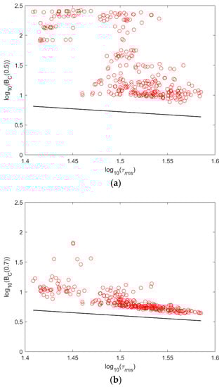
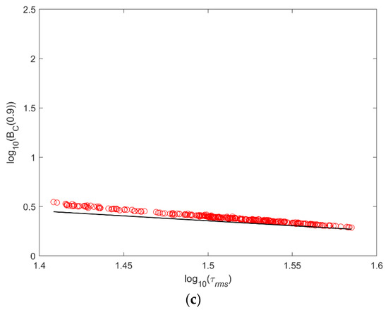
Figure 1.
Relationship between pairs of values (τrms, BC) for different frequency correlation levels, cf. (a) cf = 0.5. (b) cf = 0.7. (c) cf = 0.9. Bc: coherence bandwidth; τrms: root mean square delay spread.
4.2. Application Examples
As an initial application example, the values of the ChB length (NC) obtained for the lower bound Equation (15) are analyzed for two bands of interest in 5G, those centered on 3.6 GHz and 26 GHz. For each band, indoor and outdoor scenarios are considered, as well as two typical situations of low mobility (pedestrian), and high speed (vehicular). Table 1 shows the parameters defining the six propagation environments considered. In order to select representative values of τmax, measurements carried out by several authors in different environments have been considered. Thus, for indoor environments, values of 40 and 30 ns have been set to τmax for the 3.6 GHz [16] and 26 GHz frequency bands [17], respectively. Moreover, regarding the outdoor scenarios, values for τmax of 250 and 100 ns have been considered for the 3.6 GHz [18] and 26 GHz [19] bands, respectively. It should be noted that the proposed values are only representative and plausible values. Of course, there are many more experimental works than those referenced and site-specific values could be obtained for different propagation environments. However, the intention of this paper is to present the lower bound Equation (15), using this initial example to highlight its possibilities.

Table 1.
Parameters of the propagation environments considered.
Figure 2 presents the values of the lower bound of the ChB length (NC) obtained according to Equation (15) for different levels of frequency correlation, for the six propagation environments considered. In this case, to simplify the analysis of the results, the temporal correlation level (ct) has been prefixed to 0.7. It can be seen how the length of the ChB decreases as the correlation level of BC increases according to the arccos(cf) function, and the value cf = 0.7 can be considered a breaking point from which the slope of the curves increases. The effect of the different dispersion of the channels is also observed, as there is a reduction in the length of the ChB due to the increase in the delay spread of the outdoor channel compared to the indoor one. Furthermore, it must be added that a greater dispersion takes place in the 3.6 GHz band compared to the 26 GHz one. Finally, the effect of the speed of the users is also observed. The increase in speed between a user who moves on foot compared to another who travels in a vehicle at high speed produces, as is well known, a drastic decrease in the length of the ChB. Table 2 shows the NC values obtained for the representative frequency correlation levels, cf, of 0.5, 0.7 and 0.9. The NC values presented in the table, i.e., the minimum number of samples in the ChB, show variations of up to three orders of magnitude in different propagation environments and for the two frequency bands, also and very importantly, with the degree of correlation adopted for the definition of BC.
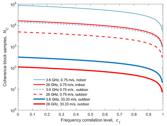
Figure 2.
Coherence block (ChB) lower bound for different levels of frequency correlation in the six propagation environments considered, and for a time correlation level of 0.7.
Table 2.
ChB lower bound length for representative frequency correlation levels, 0.5, 0.7 and 0.9.
In Figure 3, the variation of NC is represented against the correlation coefficients in frequency and time, but now varying these together according to Equation (15). Only the most critical case of a channel with a high mobility has been considered. The significant increase in NC that can be achieved if lower correlation values are set for both domains is shown. This example shows the interest in developing channel estimators that are capable of working with pilots spaced in time and frequency as much as possible. In addition, research on M-MIMO precoding and combining schemes that support the outdated channel state information (CSI) as best as possible also plays a key role.
Figure 3.
ChB lower bound as a function of both correlation coefficients, in frequency and time. The outdoor in car cases have been considered.
In order to complete the analysis and show the validity of the lower bound proposed in Equation (15), that limit is applied to semi-empirical values of ChB lengths. To make a complete measurement of the length of the ChB in a specific environment, it is necessary to measure BC and TC for a set of sampling points in that environment. In our case, we have a wide set of BC measurements carried out in an indoor environment in the 3.2–4 GHz frequency band, already presented in [20]. However, we do not have measurements concerning the TC values in this environment, since the measurements in [20] were made for another purpose. To solve this problem, we propose a semi-empirical approach consisting of setting a theoretical value for TC, obtained from the Clarke’s model, calculated according to Equation (8). The TC obtained takes a value of approximately 20 ms, corresponding with a coherence time at a correlation level of ct = 0.7 [12], for a typical indoor speed of 0.75 m/s, and at the central band frequency of 3.6 GHz.
Figure 4 presents the cumulative distribution function (CDF) of the estimated NC for the frequency correlation levels (cf) of 0.5, 0.7 and 0.9. The results included show experimentally the validity of the lower bound for a real indoor channel, and they highlight the random nature of NC. The semi-empirical results are compared with the lower bound calculated according to Equation (15). It can be observed that the lower bound proposed by the authors in Equation (15) is conservative but can be used as an initial useful approach to establish the ChB length.
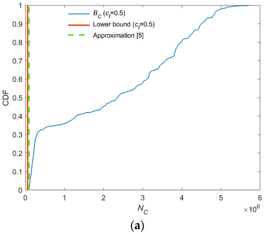
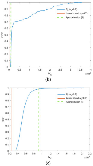
Figure 4.
Analysis with experimental results of both the lower bound proposed and an approximation given in [5]. Cumulative distribution function (CDF) of the NC = BCTC considering the values of BC obtained from indoor channel measurements [20] for different frequency correlation levels, cf (ct = 0.7). (a) cf = 0.5. (b) cf = 0.7. (c) cf = 0.9.
Furthermore, the value obtained following the rule-of-thumb proposed in [5] (remark 2.1) is also represented in Figure 4. The value of TC is estimated as λ/4v, and BC as 1/2Td, where Td is the delay spread, the delay difference between the shortest and longest path in the PDP. According to the measurements [20], an average value for the Td parameter would be 150 ns in the indoor environment considered. Therefore, the ChB length (BCTC) takes a value of 92,592 samples, which is the limit represented with a dash line in Figure 4. It is remarkable that this value is a deterministic estimate and thus, it does not consider the level of coherence for which it is defined. In Figure 4, it can be seen that it is a reasonable estimate when NC is defined for frequency correlation levels of 0.5; in fact, at least in this case, it behaves like the lower bound proposed; but it leads to an overestimation of the length of ChB for correlation levels of 0.7 and 0.9. For cf = 0.7, it is observed that 19% of the values are below the one predicted by the rule-of-thumb; and for cf = 0.9, practically all the values (99%) are below the approach.
5. Conclusions
Starting from the uncertainty relations obtained by Fleury, a lower bound has been derived for the length of the ChB. The bound explicitly relates to basic parameters of the channel, such as the maximum expected RMS delay spread, the carrier frequency as well as mobile speeds. Moreover, the dependence of the length of the ChB on the selected correlation levels in order to define both BC and TC, is quantified. Results for typical indoor as well as outdoor wireless situations (pedestrian and vehicular users) in the 3.6 and 26 GHz, along with those provided for experimental indoor data in the 3.2–4 GHz, show the validity of the lower bound presented. It must be pointed out that the impact of the correlation levels on the outdating of channel estimation is an aspect that must be analyzed in detail in future works.
The high dispersion of the values of channel parameters such as the BC, TC, τrms and vrms along a propagation environment, underlines the need to consider the duration of the ChB as a random variable, and to analyze it from a statistical point of view, obtaining probability distributions that should allow us to obtain outage values, beyond a boundary that allows 100% compliance to be ensured but whose tightness is low. However, since the overhead in channel estimation in future mobile communication systems, especially in systems based on massive MIMO technology, depends on the length of the ChB, the proposed lower bound is a valuable engineering tool for assisting in the design and sizing of the physical layer.
Author Contributions
Conceptualization, R.P.T.; methodology, J.R.P. and R.P.T.; software, J.R.P.; validation, J.R.P. and R.P.T.; formal analysis, R.P.T.; data curation, J.R.P.; supervision, R.P.T., writing—original draft preparation, J.R.P. and R.P.T. All authors have read and agreed to the published version of the manuscript.
Funding
This work has been supported by the Spanish Ministry of Economy, Industry and Competitiveness (TEC2017-86779-C2-1-R).
Data Availability Statement
Not applicable.
Conflicts of Interest
The authors declare no conflict of interest.
References
- Marzetta, T.L. How Much Training is Required for Multiuser Mimo? In Proceedings of the 2006 Fortieth Asilomar Conference on Signals, Systems and Computers, Pacific Grove, CA, USA, 29 October–1 November 2006; pp. 359–363. [Google Scholar]
- Marzetta, T.L. Noncooperative Cellular Wireless with Unlimited Numbers of Base Station Antennas. IEEE Trans. Wirel. Commun. 2010, 9, 3590–3600. [Google Scholar] [CrossRef]
- Björnson, E.; Larsson, E.G.; Marzetta, T.L. Massive MIMO: Ten myths and one critical question. IEEE Commun. Mag. 2016, 54, 114–123. [Google Scholar] [CrossRef]
- Bjornson, E.; Larsson, E.G.; Debbah, M. Massive MIMO for Maximal Spectral Efficiency: How Many Users and Pilots Should Be Allocated? IEEE Trans. Wirel. Commun. 2016, 15, 1293–1308. [Google Scholar] [CrossRef]
- Björnson, E.; Hoydis, J.; Sanguinetti, L. Massive MIMO Networks. In Massive MIMO Networks: Spectral, Energy, and Hardware Efficiency; Now Publisher: Delft, The Netherlands, 2019; Chapter 2; pp. 219–220. [Google Scholar]
- Fleury, B. An uncertainty relation for WSS processes and its application to WSSUS systems. IEEE Trans. Commun. 1996, 44, 1632–1634. [Google Scholar] [CrossRef]
- Bello, P. Characterization of Randomly Time-Variant Linear Channels. IEEE Trans. Commun. 1963, 11, 360–393. [Google Scholar] [CrossRef]
- Parsons, J.D. Wideband channel characterization. In The Mobile Radio Propagation Channel, 2nd ed.; John Wiley & Sons: Chichester, UK, 2000; Chapter 6; pp. 164–189. [Google Scholar]
- Gans, M. A power-spectral theory of propagation in the mobile-radio environment. IEEE Trans. Veh. Technol. 1972, 21, 27–38. [Google Scholar] [CrossRef]
- Varela, M.; Sánchez, M.G. RMS delay and coherence bandwidth measurements in indoor radio channels in the UHF band. IEEE Trans. Veh. Technol. 2001, 50, 515–525. [Google Scholar] [CrossRef]
- Howard, S.; Pahlavan, K. Measurement and analysis of the indoor radio channel in the frequency domain. IEEE Trans. Instrum. Meas. 1990, 39, 751–755. [Google Scholar] [CrossRef]
- Steele, R.; Hanzo, L. Mobile radio channels. In Mobile Radio Communications, 2nd ed.; Wiley: Chichester, UK, 1999; Chapter 2; pp. 91–118. [Google Scholar]
- Bracewell, R. The Fourier Transform and Its Applications. Am. J. Phys. 1966, 34, 712. [Google Scholar] [CrossRef]
- Zollinger, E. Measured inhouse radio wave propagation characteristics for wideband communication systems. In Proceedings of the 8th European Conference on Electrotechnics, Conference Proceedings on Area Communication, Stockholm, Sweden, 13–17 June 1988; pp. 314–317. [Google Scholar]
- Moraitis, N.; Kanatas, A.; Pantos, G.; Constantinou, P. Delay spread measurements and characterization in a special propa-gation environment for PCS microcells. In Proceedings of the IEEE 2002 International Symposium on Personal, Indoor and Mobile Radio Communications, Lisboa, Portugal, 5–18 September 2002; pp. 1190–1194. [Google Scholar]
- Perez, J.R.; Torres, R.P.; Rubio, L.; Basterrechea, J.; Domingo, M.; Penarrocha, V.M.R.; Reig, J.; Perez, J.R.; Basterrechea, J.; Rodrigo, V.M. Empirical Characterization of the Indoor Radio Channel for Array Antenna Systems in the 3 to 4 GHz Frequency Band. IEEE Access 2019, 7, 94725–94736. [Google Scholar] [CrossRef]
- Rubio-Arjona, L.; Torres, R.P.; Rodrigo-Peñarrocha, V.M.; Pérez, J.R.; González, H.A.F.; Molina-Garcia-Pardo, J.-M.; Reig, J. Contribution to the Channel Path Loss and Time-Dispersion Characterization in an Office Environment at 26 GHz. Electronics 2019, 8, 1261. [Google Scholar] [CrossRef]
- Wang, Z.; Wang, P.; Li, W.; Xiong, H. Wideband Channel Measurements and Characterization of the Urban Environment. In Proceedings of the 2007 International Symposium on Microwave, Antenna, Propagation and EMC Technologies for Wireless Communications, Hangzhou, China, 16–17 August 2007; pp. 826–829. [Google Scholar]
- Rappaport, T.S.; MacCartney, G.R.; Samimi, M.K.; Sun, S. Wideband Millimeter-Wave Propagation Measurements and Channel Models for Future Wireless Communication System Design. IEEE Trans. Commun. 2015, 63, 3029–3056. [Google Scholar] [CrossRef]
- Pérez, J.R.; Torres, R.P.; Domingo, M.; Valle, L.; Basterrechea, J. Analysis of Massive MIMO Performance in an Indoor Picocell With High Number of Users. IEEE Access 2020, 8, 107025–107034. [Google Scholar] [CrossRef]
Publisher’s Note: MDPI stays neutral with regard to jurisdictional claims in published maps and institutional affiliations. |
© 2021 by the authors. Licensee MDPI, Basel, Switzerland. This article is an open access article distributed under the terms and conditions of the Creative Commons Attribution (CC BY) license (http://creativecommons.org/licenses/by/4.0/).