Vehicular Visible Light Positioning Using Receiver Diversity with Machine Learning

Abstract

This paper proposes a 2-D vehicular visible light positioning (VLP) system using existing streetlights and diversity receivers. Due to the linear arrangement of streetlights, traditional positioning techniques based on triangulation or similar algorithms fail. Thus, in this work, we propose a spatial and angular diversity receiver with machine learning (ML) techniques for VLP. It is shown that a multi-layer neural network (NN) with the proposed receiver scheme outperforms other ML algorithms and can offer high accuracy with root mean square (RMS) error of $0.22$ m and $0.14$ m during the day and night time, respectively. Furthermore, the NN shows robustness in VLP across different weather conditions and road scenarios. The results show that only dense fog deteriorates the performance of the system due to reduced visibility across the road.

1. Introduction

In the past decade, there has been high interest and development in the field of intelligent vehicles. Numerous intelligent vehicles systems have been proposed to improve road safety and reduce traffic congestion. The unremitting research outputs have led to the development of various driver assistant systems such as cooperative adaptive cruise control, lane changing, lane-keeping and highway driver assistant systems. The practicality of these systems requires autonomous vehicles to have efficient control functionality, communication, precise localisation and perception to identify their surroundings and relevant obstacles [1]. The existing driver assistant systems are restricted to only assisting the driver, knowing that the driver is responsible for the overall vehicle control or in some cases fully autonomous under certain conditions. Several challenges arise in anticipation of deploying fully autonomous vehicles. One of these challenges for fully autonomous vehicles is to achieve absolute and accurate positioning.

Global navigation satellite systems (GNSS) are widely adopted due to its compatibility and coverage. However, GNSS signals suffers from outages in metropolitan areas, under dense tree canopies, tunnels, bridges and near tall buildings where the line of sight propagation path is blocked [2]. Furthermore, solar flaring activities in the ionospheric layer of the earth’s surface, temperature, pressure, density or humidity changes within the tropospheric layer of the earth’s surface can affect the accuracy of GNSS [3]. This, in turn, prompts the need for more accurate positioning techniques to co-exist with GNSS.

The wide availability and popularity of solid-state lighting (SSL) such as light-emitting diodes (LEDs) for outdoor and indoor illumination, display, and traffic signalling, provides the opportunity to utilise them for accurate positioning and high-speed communication [4]. The rapid deployment of LED street lights in compliance with the current energy-saving schemes funded by the European Commission, opens a platform of opportunities for outdoor visible light positioning (VLP) especially in tunnels and underground roads. Generally, VLP is based on received signal strength (RSS) [5,6,7,8], time of arrival (TOA), time difference of arrival (TDOA) [9,10] or angle of arrival (AOA) algorithms [11]. Different methodologies such as triangulation, proximity and fingerprinting are considered in these algorithms. At least three spatially non-collinear distributed transmitters are required to predict the position with these algorithms.

VLP has been shown to provide accurate positioning in indoor environments [7,8,12]; however, there are limited studies conducted on its application to outdoor environments. A VLP technique using tunnel infrastructure and car tail lamp was demonstrated in [5]. The study used a camera sensor receiver and image processing to extract information for positioning; however, it was based on the assumption that there is always a neighbouring car on the road, several meters ahead, continuously sending its updated position information. A TDOA approach to VLP is conducted in [6] for vehicle applications using traffic light and two photodiodes (PDs). This TDOA application, however, required time synchronization among traffic lights which may be difficult in heterogeneous environments. Furthermore, the receivers required large separation (2 m in the aforementioned study, which is not practical in all cases) for accurate positioning. Moreover, the algorithm is only applicable if inbound and outbound vehicles are assumed to have a constant speed. The feasibility of using streetlights for positioning using two rolling shutter CMOS sensors was shown in [13]; however, the streetlight setup adopted in the study was a two-sided streetlight in a single two-lane road, thus providing distributed transmitter setup. The ability to exploit signal from both side of the road relaxed the collinearity condition and allowed the system to exploit trilateration. Moreover, the accuracy of the system was affected by the blooming effect, which causes the LED images to be less clear in real-life applications.

The streetlight design is heterogeneous and the previously mentioned VLP algorithms require specific design. Most importantly, these algorithms will not work when the streetlights are not distributed. Hence, for VLP to work universally in all the streets, an algorithm must be developed, which works in the worst-case scenario, where the streetlights are located in a linear array on only one side of the road. In our previous work [14], we proposed the use of receiver diversity and supervised artificial neural network (ANN) to solve this aforementioned issue. We extended the work in [14] by using spatial and angular diversities with different machine learning (ML) approaches such as simple recurrent neural network (sRNN), gated recurrent unit (GRU) and long short term memory (LSTM) [15] to accurately estimate the position irrespective of the relative locations of the streetlights and further explore the effect of different weather conditions. To the best of the authors’ knowledge, this paper is the first study of VLP with a linear array of streetlights using receiver diversity for autonomous vehicle and other outdoor applications. The contributions of this paper are threefold. Firstly, we propose the use of spatial and angular receiver diversity to mitigate the effect of collinearity in VLP. Secondly, this paper exploits the versatility of ML algorithms to improve system performance in VLP and further compare their respective performances on the same collinear scenarios. Finally, the effect of weather conditions on VLP in the collinear scenario is studied.

The rest of the paper is organised as follows: the system description is provided in Section 2. Section 3 describes the proposed application of ML for 2-D localisation. The performance of the proposed system using ML is discussed in Section 4. Finally, conclusions are drawn in Section 5.

2. System Description

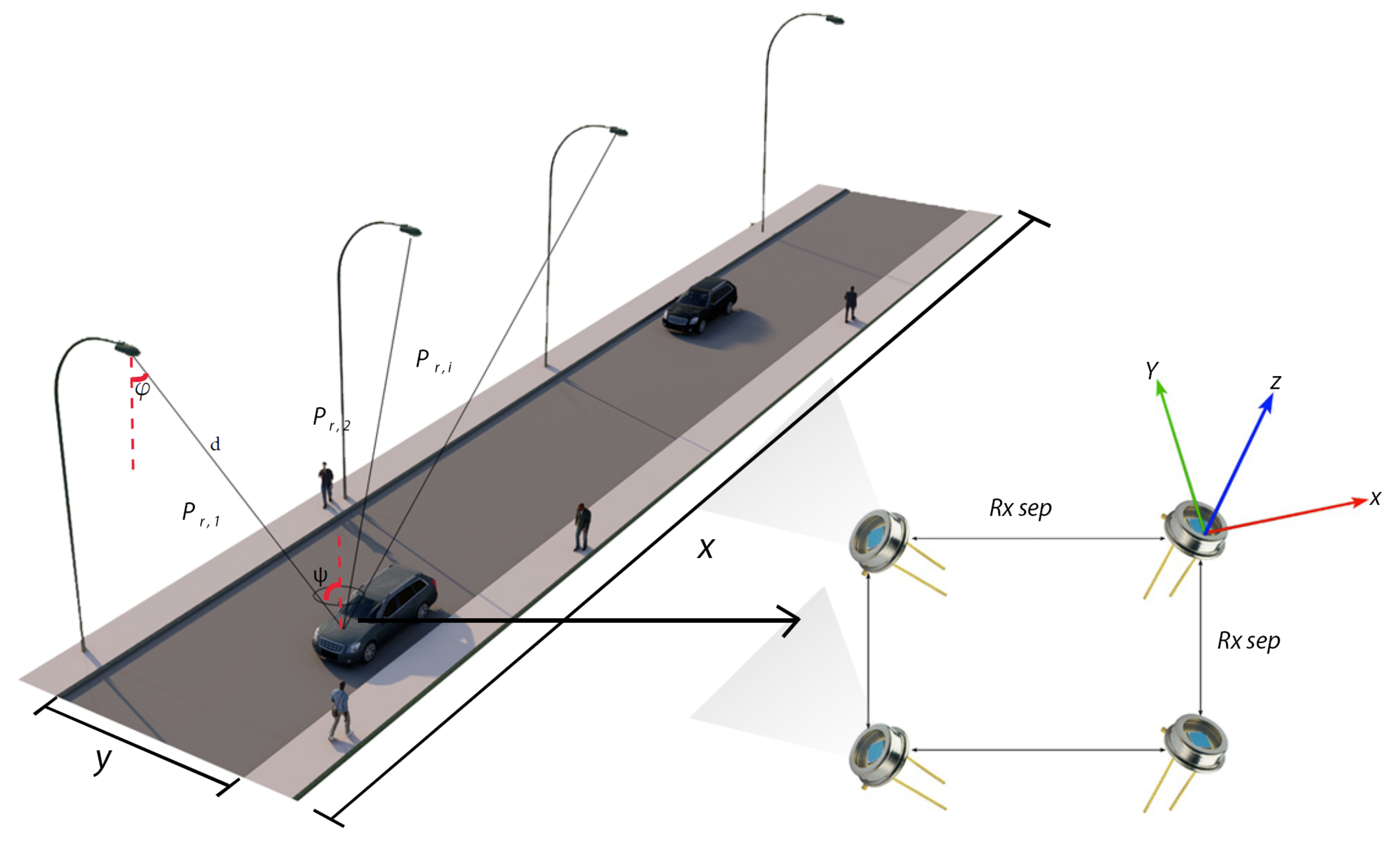
The proposed VLP system architecture with streetlights and the receiver system with spatial and angular diversity is shown in Figure 1. Streetlights are installed at the side of the road as transmitters. It is assumed that each transmitter transmits time division multiplex (TDM) or frequency division multiplex (FDM) signals as outlined in [16]. The receivers are located on a vehicle that moves along the x-axis and changes lane across the y-axis. The vehicles are assumed to travel on a tarmac road with a gradient close to zero; therefore, the vehicle’s motion along the x and y-axis are significantly larger than the displacement along the z-axis. Consequently, we only consider two degrees of movement along the x-axis and y-axis and hence focus on 2-D localisation. Figure 1 also shows the receiver system, which consists of multiple photodiodes (PDs), pointed in different directions. Note that, tilting angles are independent for each PD and optimised for vehicular VLP in Section 4.2. The main parameters that was used for the simulation are shown in Table 1 [17,18].

Figure 1. Schematic of VLP using streetlight. Schematic of spatial and angular diversity receiver.

Table 1. Parameters used for simulation [17,18].

Parameter	Value
Background current $\left(I_{bg}\right)$ [mA]	5.1
FET channel noise factor ($\Gamma$)	1.5
FET trans-conductance ($g_m$) [mS]	30
Fixed capacitance of PD ($\eta$) [pF/cm${}^2$]	112
No. of receiver (N)	4
Noise bandwidth factor $\left(I_2\right)$	0.562
Noise bandwidth factor $\left(I_3\right)$	$0.0868$
Noise bandwidth, $\left(B\right)$ [MHz]	1
Number of transmitters (M)	3
Optical filter gain (G)	1
Receiver area, $\left(A\right)$ [cm${}^2$]	1
Road parameters $(L\times W)$ [m]	$60\times 5$
Temperature ($T_k$) [K]	295
Transmitter height [m]	7
Transmitter power $\left(P_t\right)$ [W]	90
Transmitter semi-angle (${\varphi }_{1/2}$) [degree]	60
Transmitter spacing [m]	30

Given that the innate parameters of the PDs such as the area and responsivity are known, the received power $P_{r,i}$ at various locations across the road can be calculated as follows:

$$P_{r,i}=H_{los}\left(0\right)P_{t,i}{\beta }_{\lambda }$$

(1)

where $H_{los}\left(0\right)$ is the line-of-sight (LOS) DC channel gain between the PD and the ith LED, $P_{t,i}$ is the transmitted power from the ith LED and ${\beta }_{\lambda }$ is the atmospheric attenuation due to different weather conditions. As the receiver is pointing away from the road surface, the non-LOS link is not considered in the study. The LOS channel DC gain is given as:

$$H_{los}\left(0\right)=\left\{\begin{array}{c}\frac{(m+1)A}{2\pi d^2}{\cos }^m\left(\varphi \right)T_s\left(\varphi \right)g\left(\psi \right)\cos \left(\psi \right)0\le \psi \le {\mathrm{\Psi }}_c\hfill \\ 0,\hspace{1em}\hspace{1em}\hspace{1em}\hspace{1em}\hspace{1em}\hspace{1em}\hspace{1em}\psi >{\mathrm{\Psi }}_c\hfill \end{array}\right.,$$

(2)

where A is the PDs physical area, $T_s\left(\psi \right)$ is the filter gain, $g\left(\psi \right)$ is the optical concentrator gain, $\psi$ is the angle of incidence, ${\psi }_c$ is the PDs field of view, $\varphi$ is the irradiance angle, d is the distance between the receiver and the transmitter and m is the Lambertian emission order given by:

$$m=\frac{-\ln 2}{\ln (\cos {\varphi }_{1/2})},$$

(3)

where ${\varphi }_{1/2}$ represents the half-power angle of the LED. The optical concentrator gain is calculated as:

$$g\left({\psi }_i\right)=\frac{n_c^2}{{\sin }^2\mathrm{\Psi }},$$

(4)

where $n_c$ is the refractive index of the concentrator.

Furthermore, among the various atmospheric conditions that cause signal attenuation, fog is considered to contribute the most severe attenuation [17]. The atmospheric attenuation due to fog is related to the visibility V, in km, and wavelength $\lambda$. Using the empirical approach, the relationship between V and the fog attenuation given by the Kim model [17] as:

$$V=\frac{10{\log }_{10}{T}_{th}}{{\beta }_{\lambda }}{\left(\frac{\lambda }{{\lambda }_0}\right)}^{-w},$$

(5)

where $T_{th}$ is the $2\%$ visual threshold, w is the particle size distribution coefficient and ${\lambda }_0$ is the solar band maximum spectrum, where ${\lambda }_0=550$ nm in this paper. The fog attenuation is estimated using Kims model from the w value and visible–NIR wavelengths, which is a function and V and is defined as [17]:

$$w=\left\{\begin{array}{c}1.6\mathrm{for}V>50\mathrm{km}\hfill \\ 1.3\mathrm{for}6\mathrm{km}<V<50\mathrm{km}\hfill \\ 0.16V+0.34\mathrm{for}1\mathrm{km}<V<6\mathrm{km}\hfill \\ V-0.5\mathrm{for}0.5\mathrm{km}<V<1\mathrm{km}\hfill \\ 0\mathrm{for}V<0.5\mathrm{km}\hfill \end{array}\right.$$

(6)

Table 2 shows the visibility range under different weather conditions [17].

Table 2. Weather conditions and their visibility range values [17,19].

Weather Condition	Visibility Range (m)
Dense fog	[$0,50$]
Thick fog	[$0,200$]
Moderate fog	[$0,500$]
Light fog	[$770,1000$]
Thin fog/heavy rain	[$1900,2000$]
Haze/medium rain	[$2800,40,000$]
Clear/drizzle	[$18,000,20,000$]
Very clear	[$23,000,50,000$]

The atmospheric attenuation is given by Beer–Lambert law as [20]:

$${\beta }_{\lambda }=\frac{\ln \frac{I_0}{I}}{d}\left[{\mathrm{km}}^{-1}\right],$$

(7)

where $I_0$ [Wm${}^{-2}$] is the optical intensity at zero distance $(d=0)$, I is the optical intensity at distance d.

The VLP is affected by thermal and shot noises, which are generally modelled as additive white Gaussian noise (AWGN). The background light and the photo-current generated by the desired signal is known as the shot noise and its variance is calculated as:

$${\omega }_{shot,i}^2=2q{I}_{bg}{I}_{2}B+2q{R}_p{P}_{r,i}B,$$

(8)

where $I_{bg}$ represents the background current, $I_2$ is a noise bandwidth factor of the current, B represents the bandwidth, q is the electronic charge and $R_p$ is the receiver responsivity. The thermal noise that arises from the amplifier at the receiver is given as:

$${\omega }_{thermal}^2=\frac{8\pi k{T}_k}{G}\eta A{I}_2{B}^2+\frac{16{\pi }^{2}k{T}_k\Gamma }{g_m}{\eta }^2{A}^2{I}_3{B}^3,$$

(9)

where k represents the Boltzmann’s constant, $T_k,G$ and $\eta$ represent absolute temperature, open-loop gain and fixed capacitance of the PD, respectively. $g_m$ and $\Gamma$ represent FET trans-conductance and FET channel noise factor, respectively.

Hence, the average signal to noise (SNR) ratio can be calculated as:

$$\overline{SNR}=\frac{1}{MN}\sum _{i=1}^M\sum _{j=1}^N\frac{{\left(P_{r-i,j}{R}_p\right)}^2}{{\omega }_{shot,j}^2+{\omega }_{thermal,j}^2},$$

(10)

where M and N are the number of transmitter and receivers, respectively.

3. Localisation Algorithms

The use of traditional localisation methods fails due to collinearity [21] caused by a linear array of transmitters for straight roads. Hence, this paper proposes the use of angular receiver diversity with ML algorithms to overcome these challenges [14], and map the received signal from the transmitter to the vehicle’s positional coordinates. Note that this research focuses on positioning in the sensor’s frame. We define the sensor’s frame as being coincident with the sensor’s (streetlight or transmitter) axis with its origin as the coordinate of the first street light $P_{r,1}$ as shown in Figure 1) and not the global (navigation frame). The results are evaluated and compared against the Cayley Menger determinant (CMD). The study in [12] uses trilateration based on CMD for positioning. The aforementioned work achieves high accuracy using LEDs and PDs without the need for extra hardware, hence making it a better model for comparison. CMD is a trilateration based algorithm that extends the cost function for positioning using RSS as described in [12]. The positioning algorithms are described in the following section.

3.1. Cayley Menger Determinant (CMD)

Using receiver diversity, the receivers position can be estimated with CMD. The received signal on the receivers are sorted from the highest to the lowest and the three strongest signals are chosen and further used for calculations. This process is considered as the localisation system covers a large area, see Figure 1. Let $\{d_{ij}:0\le i\lesssim j\le M\}$ be a set $\frac{M(M+1)}{2}$ of variables and consider the square $(M+2)\times (M+2)$ matrix where M is the number of transmitters. The CMD is defined as [22]:

$$C{M}_M:=\left|\begin{array}{cccccc}0& 1& 1& 1& \cdots & 1\\ 1& 0& d_{12}^2& d_{13}^2& \cdots & d_{1M}^2\\ 1& d_{21}^2& 0& d_{23}^2& \cdots & d_{2M}^2\\ 1& d_{31}^2& d_{32}^2& 0& \cdots & d_{3M}^2\\ ⋮& & & & \ddots & \\ 1& d_{M1}^2& d_{M2}^2& d_{M3}^2& \cdots & 0\end{array}\right|{\Gamma }_M,$$

(11)

where ${\Gamma }_M$ is the multivariate polynomial. Therefore,

det(CM${}_M$) $\in \left(Z\right)[d_{12},d_{13},\dots ,d_{(M-1)M}]$.

The CMD outputs a ($1\times 2$) vector of $(\widehat{x},\widehat{y})$ for each receiver. Further details on the application of CMD for VLP can be found in [12].

3.2. Machine Learning

In this study, four ML algorithms namely MLP, sRNN, LSTM and GRU are considered for positioning. Each neural network (NN) when trained, outputs the predicted location of the vehicle based on the input signal. The input to the NN is the received signal from the transmitter as outlined in Equation (1), and has a vector size of $(M\times N)$. The NN is trained to predict the 2-D received location. The NN has two output corresponding to predicted x and y position coordinates. The NN models investigated in this paper are briefly introduced in the following sub-sections.

3.2.1. Multi-Layer Perceptron (MLP)

MLP’s are characterised by an interconnected network of neurons capable of mapping non-linear relationships from input (received signal from the transmitter) to output (vehicle’s position coordinates). The input to the NN is computed from the bias vector and the product of the input vector and the weight matrix. The output is, however, defined by the nonlinear transformation of the sum of the neuron’s input through the use of an activation function. NNs learn through the continuous back-propagation of the predicted position errors, which consequently leads to the adjustment of the weight parameters until an optimal model is found. An adjustable momentum and learning rate can be used to prevent the MLP from becoming trapped in local minimum during back-propagation. The operation of the feed-forward layer is defined by:

$$y_t=\sigma (\Sigma x_{t}W+b),$$

(12)

where $\Sigma$ is the summation operator, $x_t$ is the input feature vector (received power from the transmitter) with vector size of $M\times N$ and $y_t$ is the predicted output vector (vehicle’s position coordinate), $\sigma$ is the sigmoid activation (non-linearity) function, $W$ is the weight matrix and $b$ is the bias vector.

3.2.2. Simple Recurrent Neural Network (sRNN)

The RNNs differs from the MLP by their ability to learn relationships within sequences. They use feedback loops, which help in connecting relationships learnt in the past. The connections are sometimes called memory. Such information learnt within the sequential dimension of the data are stored within the hidden state of the sRNN, which extends to the defined number of time steps and are mapped forward and continuously to the output. The equations governing the operation of the sRNN are:

$$h_t=\tanh (U_h{h}_{t-1}+W_x{x}_t+b_h),$$

(13)

$$y_t=\sigma (W_0{h}_t+b_o),$$

(14)

where $U_h$ is the hidden weight matrix, $b_h$ is the hidden bias vector, $b_o$ is the output bias vector, $h_{t-1}$ is the previous state, $W_x$ is the input matrix and $W_0$ is the output weight matrix. The detailed operation of the sRNN is described in [15,23].

3.2.3. Long Short-Term Memory (LSTM) Neural Network

LSTM’s are a variant of the sRNN. They were created to address the long-term dependency problems of the RNNs. Through the use of gated architectures: input gate, forget gate and output gate, LSTM can recall information from long periods of time. The gated operations of the LSTM are shown by the following equations:

$$\mathrm{forget}\mathrm{gate}:f_t=\sigma (W_f{x}_t+U_f{h}_{t-1}+b_f),$$

(15)

$$\mathrm{input}\mathrm{gate}:i_t=\sigma (W_i{x}_t+U_i{h}_{t-1}+b_i),$$

(16)

$$\mathrm{current}\mathrm{memory}\mathrm{state}:{\widehat{c}}_t=\tanh (W_c{x}_t+U_c{h}_{t-1}+b_c),$$

(17)

$$\mathrm{cell}\mathrm{state}:c_t=f_t\ast c_{t-1}+i_t\ast {\widehat{c}}_t,$$

(18)

$$\mathrm{output}\mathrm{gate}:o_t=\sigma (W_o{x}_t+U_o{h}_{t-1}+b_o),$$

(19)

$$\mathrm{final}\mathrm{memory}:h_t=o_t\ast \tanh \left(c_t\right),$$

(20)

where ∗ is the Hadamard product. $W_i$, $W_f$ and $W_c$ are the weight matrices of the input gate, forget gate and current memory state respectively, $U_i$, $U_f$, $U_c$ and $U_o$ are the hidden weight matrices of the input gate, forget gate, current memory state and output gate, respectively, and $b_i$, $b_f$ and $b_c$ are the bias vectors of the input gate, forget gate and current memory state, respectively.

3.2.4. Gated Recurrent Unit (GRU) Neural Network

Cho et al. in [24], introduced the GRU to address the vanishing gradient problem of the sRNN giving it the ability to learn long-term dependencies. Similar to the LSTM, the GRU cellular operation is characterised by gated operations; however, the GRU has its hidden state and cell state merged to form a more computationally efficient model. The operations of the GRU is governed by the following sets of equation:

$$\mathrm{update}\mathrm{gate}:z_t=\sigma (W_z{x}_t+U_z{h}_{t-1}+b_z),$$

(21)

$$\mathrm{reset}\mathrm{gate}:r_t=\sigma (W_r{x}_t+U_r{h}_{t-1}+b_r),$$

(22)

$$\mathrm{current}\mathrm{memory}\mathrm{state}:{\widehat{h}}_t=\tanh (W_h{x}_t+r_t\ast U_h{h}_{t-1}+b_h),$$

(23)

$$\mathrm{final}\mathrm{memory}:h_t=z_t\ast h_{t-1}+(1-z_t)\ast {\widehat{h}}_t,$$

(24)

where $W_h$, $W_r$ and $W_z$ are the weight matrices of the current memory state, reset gate and update gate, respectively, $U_h$, $U_r$ and $U_z$ are the hidden weight matrices of the current memory state, reset gate and update gate, respectively, and $b_h$, $b_r$ and $b_z$ are the bias vectors of the current memory state, reset gate and update gate, respectively.

4. Results and Discussion

The performance of the CMD and the ML algorithms are evaluated in this section. The VLP channel in this study is considered to be an outdoor environment. Hence the effect of sunlight and weather in all the simulations are considered unless stated otherwise. In this study, we assume that streetlights are turned on all the time. Considering the standardised illumination level of LED streetlights, the proposed VLP system is evaluated using root mean square (RMS) error, confidence interval (CI) and cumulative distributive function (CDF). The RMS error contributed independently by x and y axis are given, respectively, by:

$$RMSx=\sqrt{{(x-\widehat{x})}^2},RMSy=\sqrt{{(y-\widehat{y})}^2},$$

(25)

where $(x,y)$ is the real position and $(\widehat{x},\widehat{y})$ is the estimated position of the receivers. Hence, the combined RMS error is given by:

$$RMSerror=\sqrt{{(x-\widehat{x})}^2+{(y-\widehat{y})}^2}.$$

(26)

The CI of the RMS error is given by:

$$CI=\overline{x}\pm z\frac{s}{\sqrt{n}},$$

(27)

where $\overline{x}$ is the sample mean, z is the confidence level value, s is the sample standard deviation and n is the sample size. A 60 m long and 5 m wide road illuminated by LED streetlights 7 m high and 30 m apart, with transmitter coordinates of (0, 0, 7), (30, 0, 7) and (60, 0, 7) is considered for the initial simulation [25].

4.1. Visible Light Positioning Using CMD

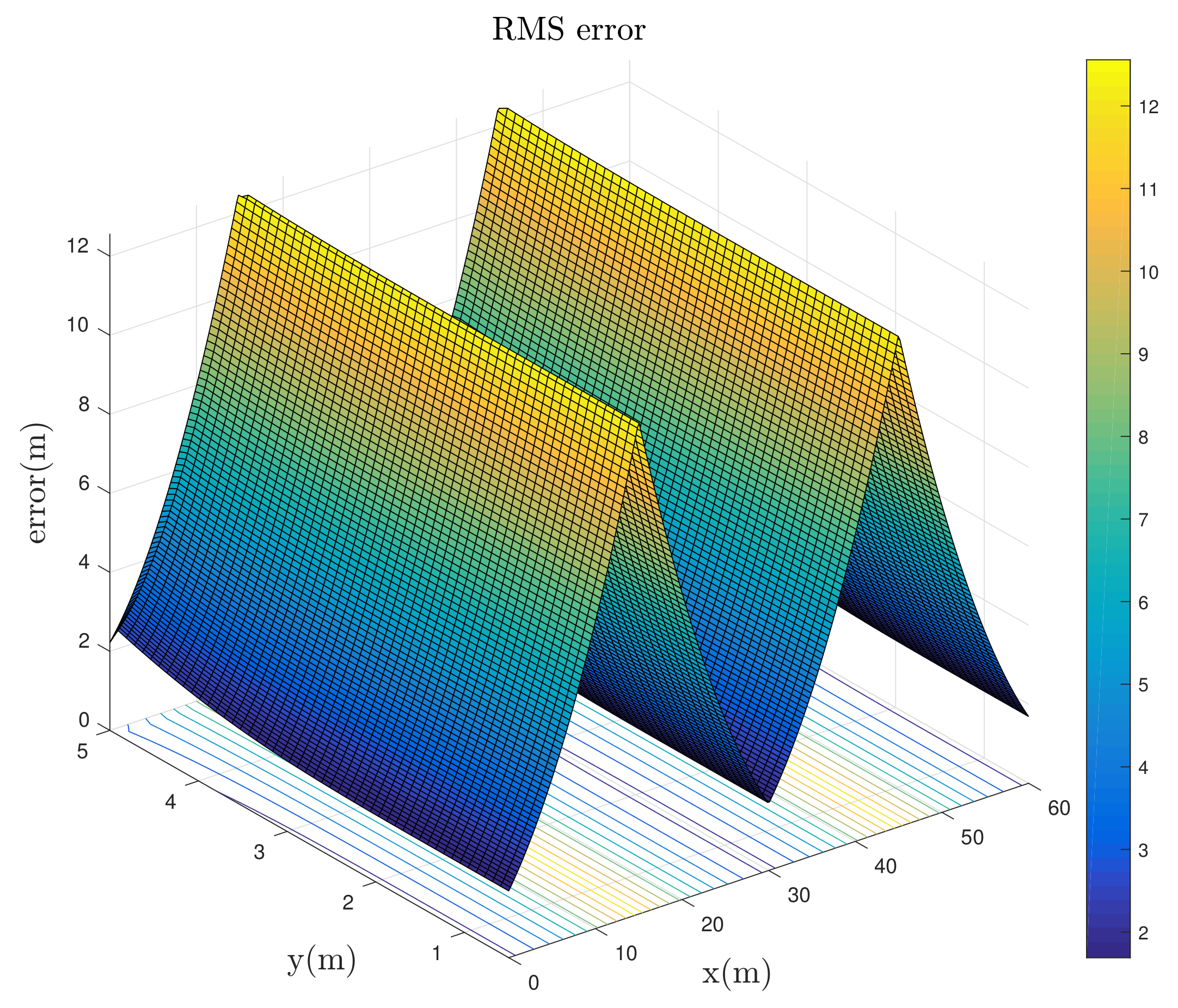
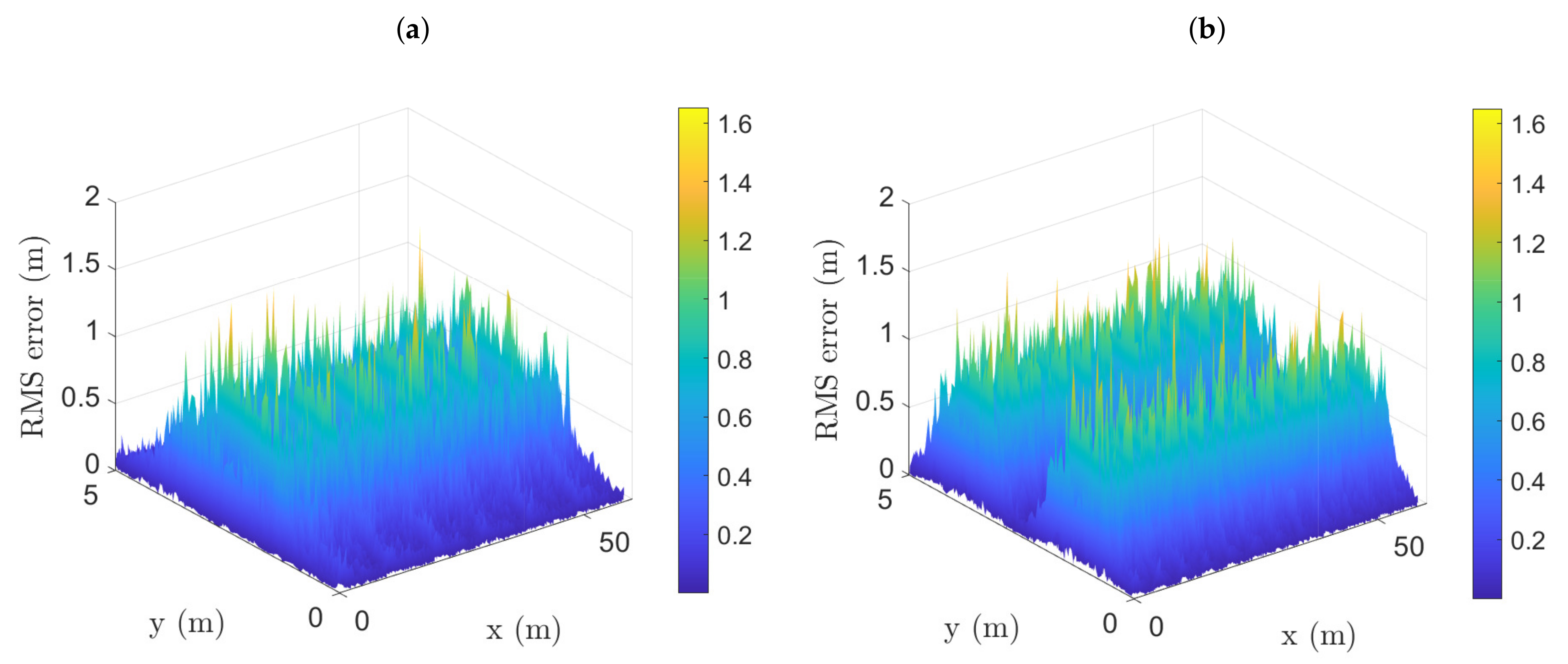
In this subsection, CMD is used to estimate the positioning error. Using a single receiver, it is impossible to estimate the positioning error due to the collinear arrangements of the streetlights. Hence, we adopt the concept of receiver diversity as shown in Figure 1. The RMS error distribution across the road using 4 receivers is shown in Figure 2. It can be seen that the localisation error is high reaching RMS error values $>12$ m. The RMS error is seen to increase at the part of the road where the signal from the third streetlight is not received adequately. It reduces as the received signal ratio between the three transmitters increases. It is noticed that the system is more accurate in the x-axis as compared to the y-axis which yielded an average RMS error of $0.95$ m and $6.77$ m, respectively. This variation in error magnitude is highly influenced by the collinearity of the transmitter. This high RMS error is not useful for the target application such as autonomous driving; therefore, to reduce the positioning error and improve the accuracy, NN-based VLP is proposed.

Figure 2. RMS error of VLP across the road using CMD.

4.2. VLP System Architecture Parameter Optimisation

Several steps are taken to optimise the NN-based VLP model ranging from the number of receivers (receiver diversity), receiver tilt angle (angular diversity), receiver spacing (spatial diversity), receiver FOV and the NN structure. First, we investigate the optimum number of receivers in the model to demonstrate the need for receiver diversity in VLP. Note that initial optimization of the VLP system structure is achieved using the MLP model in [14]. Thereafter, the NN is re-optimised. 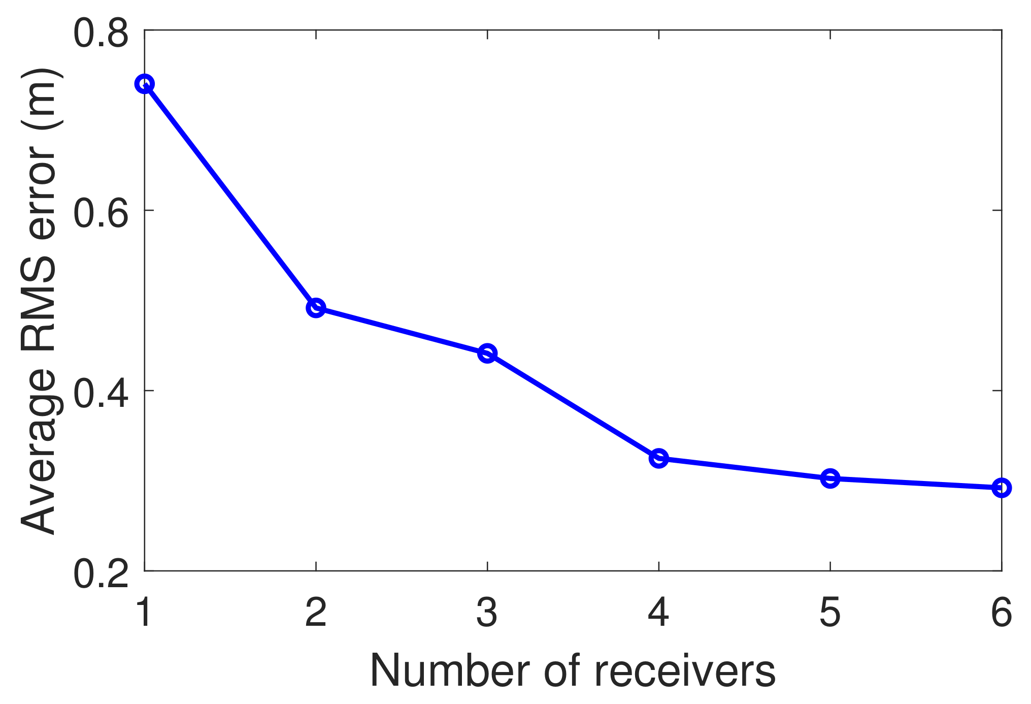Figure 3 shows the relationship between the RMS error and the number of receivers. Here, all the receivers are facing upwards. We observe that, the RMS error reduces as the number of receivers is increased. There is a significant performance improvement when the number of receivers increases from 1 to 4; however, there is a very limited improvement in performance beyond four receivers.

Figure 3. CDF of VLP as a function of the number of receivers.

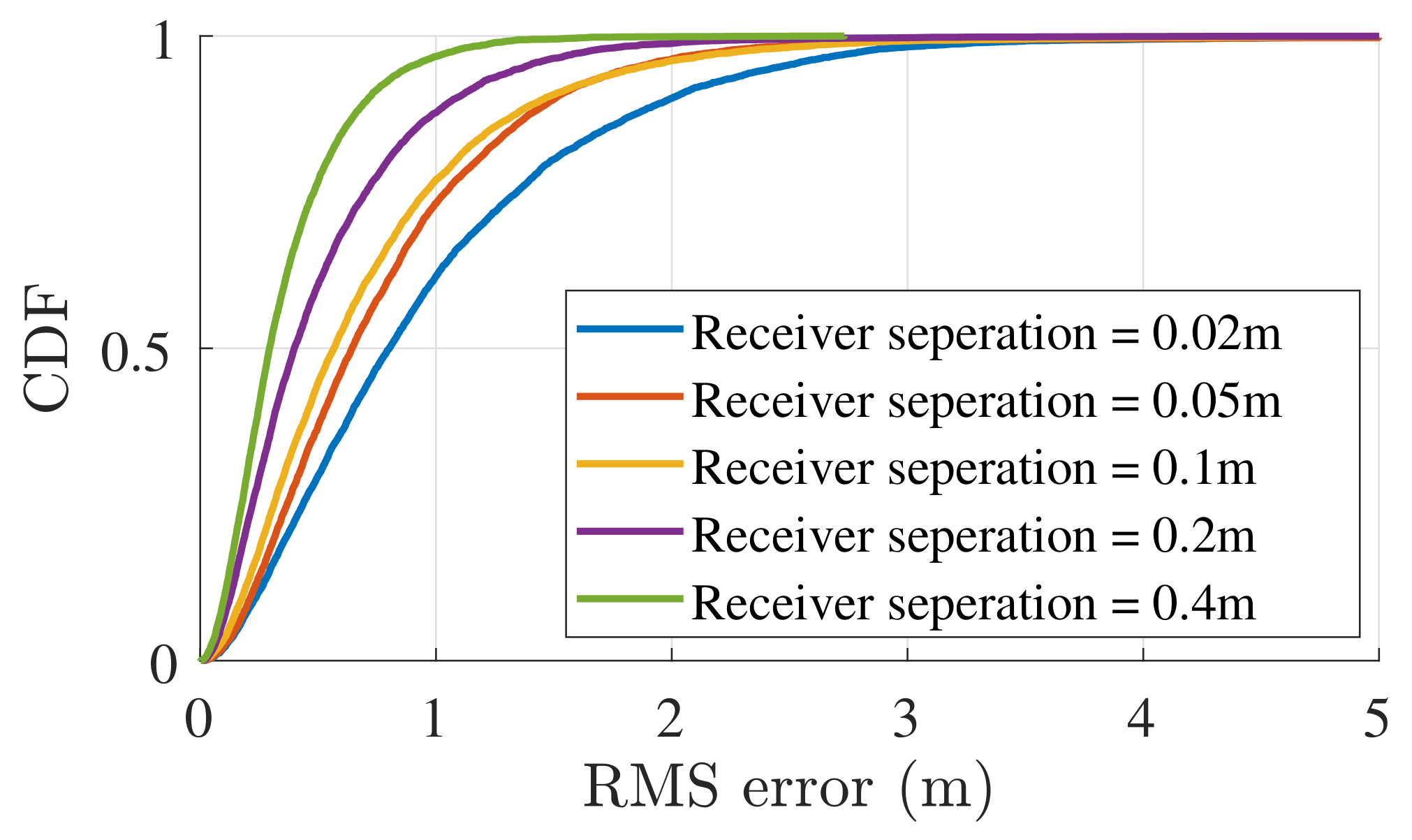
The impact of receiver separation on VLP is also investigated to select a favourable receiver spacing on the vehicle. We only consider receiver separations from $0.02$ m to $0.4$ m due to their practicality for real application. Figure 4 shows the CDF of the RMS error for the receiver separations of $0.02$ m, $0.04$ m, $0.1$ m, $0.2$ m and $0.4$ m. At $0.95$ CDF, the average RMS errors are $2.5$ m, $1.86$ m, $1.83$ m, $1.3$ m and $0.8$ m, respectively. Figure 4 illustrates that the accuracy of the system increases as the receiver spacing is increased. It is noticed that only a receiver separation of $0.4$ m (out of the chosen values) provide an RMS error below 1 m at $0.95$ CDF. Hence, the separation between the receivers of $0.4$ m is selected for further simulations.

Figure 4. CDF analysis at different receiver separation.

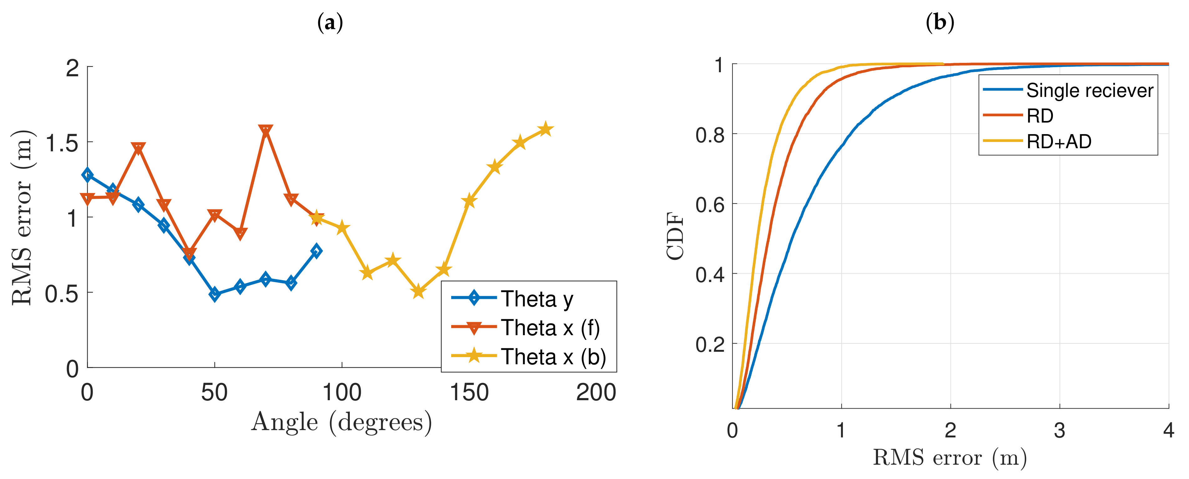
Furthermore, we consider the concept of angular diversity to improve system performance through better signal reception. In this study, the first two PDs are facing the direction of travel (forward-facing) with their angles represented as theta x (f) and the last two PDs are facing away from the direction of travel (rear-facing) with their angles labelled as theta x (b) as seen in Figure 5. The PDs are considered to have two degrees of freedom namely $\angle x$ and $\angle y$ as illustrated in Figure 1. $\angle x$ represents the rotation across the x-axis, i.e., tipping the receivers towards and away from the direction of travel. $\angle y$ represents the rotation across the y axis, i.e., tilting the receiver towards and away from the streetlight. $\angle z$ is the rotation of the PD across the z-axis. This is ignored as it does not introduce any difference to signal reception due to the circular nature of the PD. However, this could change on non-circular PDs. Starting with the forward-facing PDs, their angles are changed from $0^{\circ }$ to ${90}^{\circ }$ and the back facing PDs from ${90}^{\circ }$ to ${180}^{\circ }$ with a step size of ${10}^{\circ }$. $\angle y$ is kept constant for all the PDs so they face towards the streetlights.

Figure 5. (a) Average RMS error at different receiver tilt angle. (b) CDF analysis on the impact of receivers and angular diversity.

Figure 5a shows the RMS error with respect to receiver angles. We start by considering the forward-facing receivers. A rise in the error is first noticed when the receiver angles are tilted from $0^{\circ }$ to ${20}^{\circ }$ (Note that the rear-facing receivers and $\angle y$ are kept at ${90}^{\circ }$). The accuracy of the system is seen to improve between ${30}^{\circ }$ to ${60}^{\circ }$ with the optimum being at ${40}^{\circ }$. Next, we consider the rear-facing receivers. The RMS error is seen to reduce from ${90}^{\circ }$ to ${140}^{\circ }$ with ${130}^{\circ }$ being the optimum angle thus considering it for further simulations as the accuracy of the system decreases thereafter. It was found the RMS error decreases when $\angle y$ is tilted from $0^{\circ }$ to ${50}^{\circ }$, where it reaches a minimum. The RMS error is seen to increase beyond thereafter. Having optimised the number of receivers and their respective angles, CDF analysis is performed and presented in Figure 5b. This is to observe their respective impact to optimise the performance of the system. We start by analysing the system using a single receiver with the optimum simulation parameters. At $0.95$ CDF, an RMS error of $1.8$ m is noted. The value is seen to drop to $0.8$ m when receiver diversity is applied. Furthermore, when angular diversity is included, an RMS error of $0.72$ m is noted at $0.95$ CDF. This reduction in RMS error shows that the proposed concepts can help provide improved performance for positioning systems in outdoor applications.

4.3. Neural Network Modelling

Using the optimum vehicular VLP structure deduced in this work, we optimise different ML models to select the best fit for this application as seen in Table 3 [15,23]. The models considered are GRU, LSTM, sRNN and MLP. A total of 65,554 2-D positions were considered in the simulation studies. A subset of 1500 positions was selected randomly to tune the neural networks. $70\%$ of these positions were used for training, $15\%$ for validation and $15\%$ for testing. The GRU, LSTM and sRNN models were optimised using the Adam optimiser with an initial learning rate of 0.01, 0.01 and 0.009, respectively, as shown in Table 3. The MLP model was, however, optimised with the Levenberg–Marquardt (LM) optimiser with an initial learning rate of 0.1. The model’s parameters were initialised using the Glorot uniform kernel initialiser for all models and the orthogonal recurrent initialisers for the RNNs. The mean squared error was chosen as the loss function for the purpose of training all the models investigated. During the training of the MLP, we selected two hidden layers for regularisation purposes through the implementation of $25\%$ dropout of the units in the hidden layers. A $15\%$ dropout rate was implemented on the recurrent layers of the RNNs to prevent the models from over-fitting. We do, however, note that we found no benefit computationally and estimation wise in increasing the size of the hidden layers of all models investigated. Table 3 presents the full list of hyper-parameters for the optimised models. Furthermore, as reported in Table 3, it can be seen that the MLP outperforms the other models compared, with the lowest RMS error of $0.22$ m. The performance of the MLP compared to the other models examined suggests that the VLP is not characterised by sequential dependencies (a characteristic not known before the start of this study) and justifies the selection of the MLP for further simulations.

Table 3. Hyperparameters of the machine learning algorithms.

Training Parameters	GRU	LSTM	sRNN	MLP
Number of weights per hidden layer	16	32	32	32
Learning rate	0.01	0.01	0.009	0.1
Number of hidden layers	2	2	2	2
Activation function (hidden layers)	tanh
Kernel initialiser	Glorot Uniform
Recurrent initialiser	orthogonal
optimiser	Adam			LM
Loss function	Mean squared error
Time step	1			-
Batch size	64	32	32	0.1
Dropout rate	-			0.25
Recurrent dropout rate	0.15	0.15	0.5	-
RMS error (m)	0.26	0.26	0.29	0.22

4.4. VLP Using Angular and Spatial Diversity Receiver

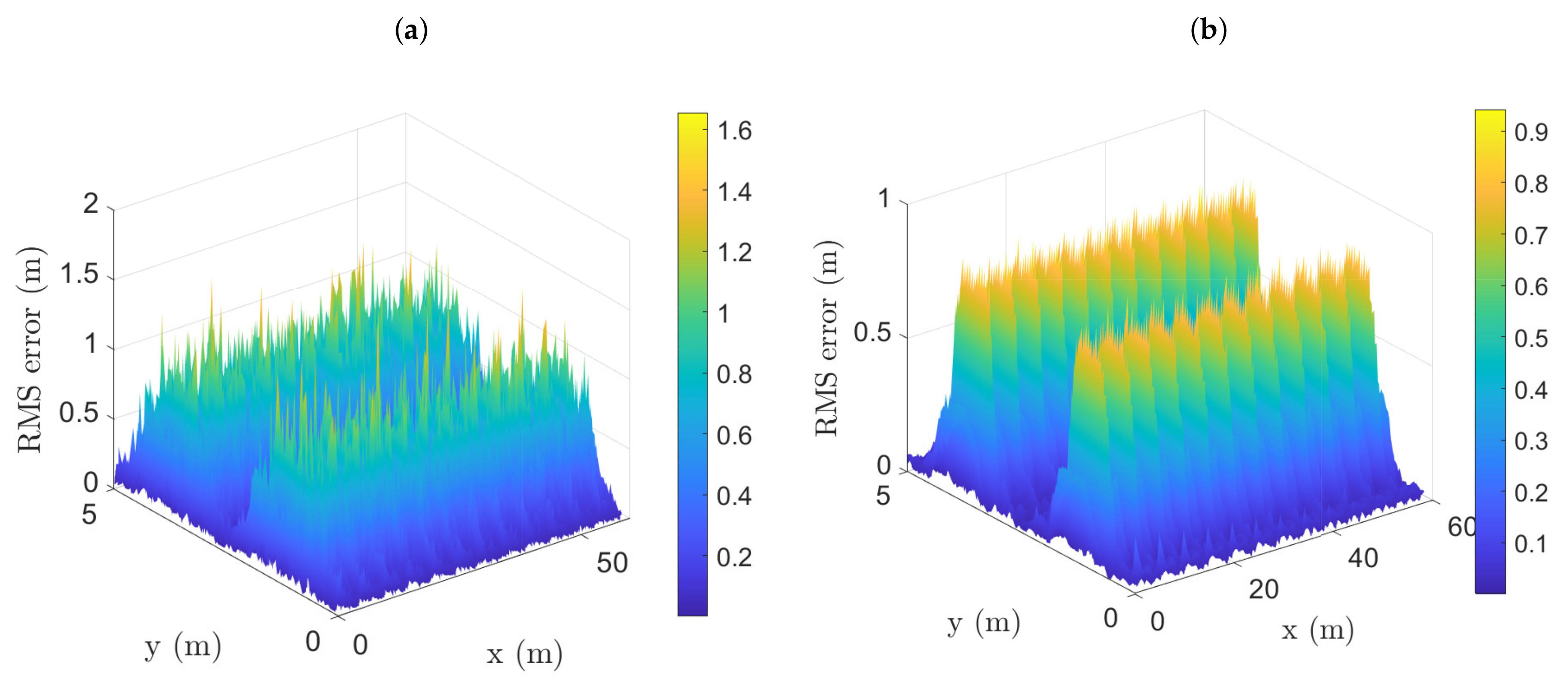
The performance of the proposed VLP system is first analysed during the day where sunlight is present unless stated otherwise. The model is simulated on a laptop computer (Intel(R) Core(TM) i7-6820HQ CPU of 2.70 GHz clock rate, 16 GB RAM and runs 64-bit Windows 10 operating system) with a computational time of 75.9ms. Each analysis was performed with over 65,554 test points. The RMS error analysis across the road is shown in Figure 6. The plot reveals the RMS error values at each point across the road. Given that the streetlights are on one side of the street (axis-$y=0$), a rise in RMS error is noticed on the other side of the road due to lower signal power reception. In the x-axis, an average RMS error of $0.02$ m is recorded. It is noticed that the average RMS error in the y-axis is $0.1743$ m, see Figure 6. Hence, the results show that the RMS error is higher in the y-axis than the x-axis. Unlike in the CMD technique, the RMS error is more evenly distributed across the road due to the learning abilities of the NN.

Figure 6. (a) x-axis RMS error distribution and (b) y-axis RMS error distribution.

Next, we compared the performance of the system during the day and at night when solar radiation is absent. Figure 7 shows the RMS error distribution across the road during the day and night. The average RMS errors are $0.22$ m and $0.14$ m during the day and night, respectively. The RMS error at night is lower than the average RMS error during the day due to reduced ambient light noise and hence improved SNR. For example, the average SNR across the road at night is 53 dB, which is 12 dB higher than the average SNR of 41 dB for the day. Similar average SNR degradation is reported in other work including simulation and measurement in [26] showing SNR degradation of $12.5$ dB for VLC. In this study, the analysis focused on the worst-case (during day) and the best case (at night); however, the performance during daytime can be improved by using a blue filter at the receiver [26], which can reduce the SNR degradation by at least 6 dB.

Figure 7. RMS error across the road: (a) during the day and (b) during the night.

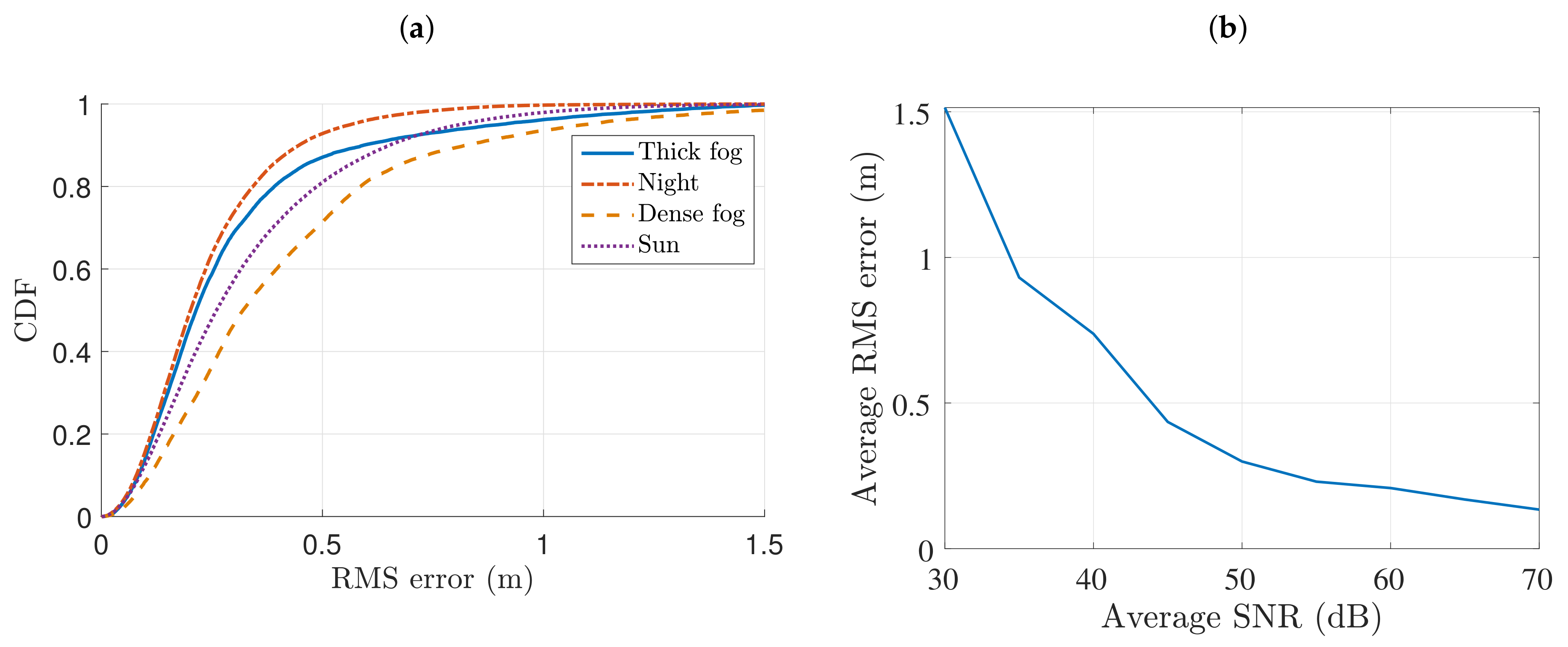
Moreover, the system’s performance is analysed over the various weather conditions, and results are presented in Figure 8a. Four representative weather conditions are selected, which are (a) sunny day time when the shot noise due to the sunlight is the strongest, (b) night when there is very low ambient noise, (c) thick fog with visibility of 200 m and (d) dense fog with visibility of 50 m when signal attenuation is very severe. The resulting average SNR across the road for these conditions are 41 dB, 53 dB, 43 dB and $36.9$ dB. Figure 8a illustrates the CDF analysis of the respective weather conditions, which reveals the best performance is obtained at night with clear weather when the noise is the minimum, followed by thick fog, sunny day time under the sun and dense fog with average RMS errors (RMS error at 0.95 CDF) of 0.14 m (0.49 m), 0.19 m (0.70 m), $0.22$ m ($0.72$ m) and $0.29$ m ($0.98$ m), respectively. As expected, the best performance is obtained at night when the received signal strength is the highest and the noise level is the lowest. The worst performance is obtained under dense fog condition when the RSS is low due to attenuation of $78.2$ dB/km. Whilst the RSS is higher for sunny days than the thick fog condition with an attenuation of $39.1$ dB/km, the performance is better with thick fog condition. This is because, in this condition, the absence of shot noise due to sunlight outweighs the attenuation due to fog. Figure 8b shows the respective RMS error analysis at different SNR values starting from 30 dB to 70 dB during the day. The model yields RMS error values above $0.4$ m until it reaches 46 dB. Further drop in RMS error is noticed from 46 dB to 60 dB where an average RMS error below $0.19$ m is achieved. Thereafter, no significant change in the gradient is noticed until an average RMS error of $0.13$ m is recorded at 70 dB.

Figure 8. (a) CDF of VLP at different weather conditions and (b) average SNR versus average RMS error.

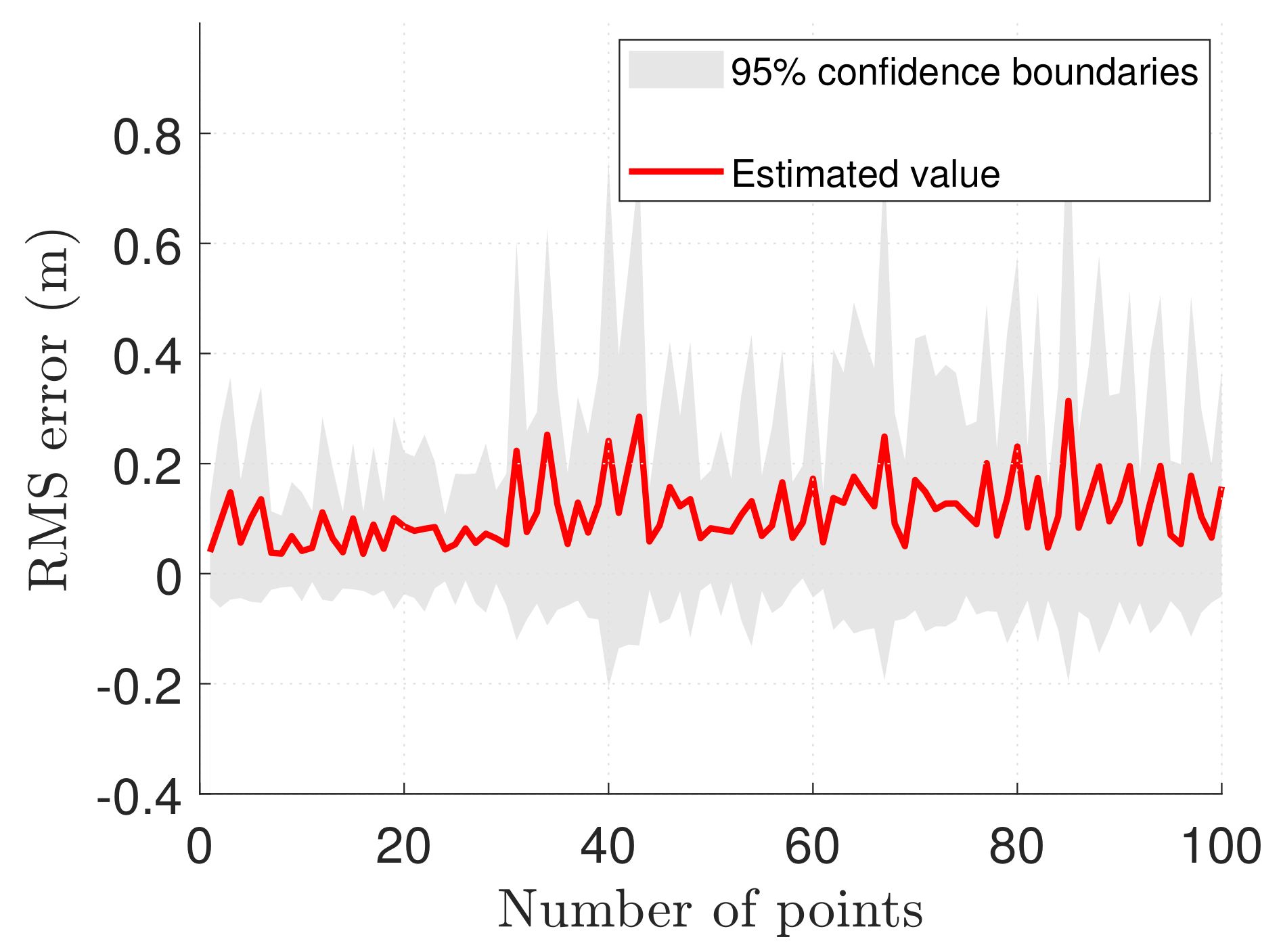
CI is used to display the upper and lower boundaries of the given RMS error. Given that z is $95\%$ and n is 100, Figure 9 shows the error boundaries for the same vehicle position per point taken over 100 different data sets, which was conducted during the day. It can be seen that most of the estimated value falls under $0.3$ m with an upper error boundary averaging $0.4$ m; however, a few points have an upper error boundary higher than $0.6$ m (see Figure 9). This is caused by the lower SNR values across the road.

Figure 9. CI analysis over 100 positions across the road.

Finally, the performance of the VLP model is investigated with five different road scenarios and LED streetlight setup as presented in most urban cites shown in Table 4 [27]. Note that case I is the dimension the initial study is based on. All the scenarios are analysed based on average RMS error and (RMS error at $0.95$ CDF). By comparing Case I and Case II, reducing the transmitter spacing and the road width improves system performance. In Case III, streetlights are located on both sides of the road. Though the transmitter setup is distributed, the link distance is still long with 20 m transmitter spacing and 15 m wide road. When a 5 m reduction is made on both the transmitter spacing and road width and despite increasing the transmitter height by 1 m as seen in Case IV, the performance of the system increases by $67\%$. Using the same transmitter height but increasing the transmitter spacing to 30 m in Case V provides similar performance in Case III. The system performs better on smaller roads and providing a distributed transmitter (double-sided) enhances system performance.

Table 4. Different road dimensions in urban cities.

	Height	Spacing	Road Width	Transmitter Position	Average RMS Error	RMS Error at $95\%$ CI
Case I	7 m	30 m	5 m	Single sided	$0.22$ m	$0.72$ m
Case II	7 m	15 m	5 m	Single-sided	$0.16$ m	$0.67$ m
Case III	7 m	20 m	15 m	Double-sided	$0.27$ m	$0.97$ m
Case IV	8 m	15 m	10 m	Double-sided	$0.09$ m	$0.29$ m
Case V	8 m	30 m	10 m	Double-sided	$0.27$ m	$1.21$ m

5. Conclusions

This paper has presented a novel vehicular VLP solution based on MLP using the spatial and angular diversity receiver. Detailed system optimisation is presented ranging from the number of receivers, receiver angles and receiver separation. By using four PDs at the receiver end, their combined received signal is used to calculate their respective distances to the transmitter. Using CMD, the model yielded an average RMS error of $6.84$ m under direct sunlight condition. ML algorithms were later investigated with MLP offering the best performance with an average RMS error of less than $0.27$ m. Furthermore, the system performance was tested under different weather conditions to show the capability of the system in adverse weather conditions. In clear weather, dense fog and at night, the system yielded an average RMS error of $0.22$ m, $0.29$ m and $0.14$ m, respectively. This work proves that MLP with spatial and angular diversity receiver can overcome the collinearity condition in VLP. Future work includes the practical implementation of the proposed system and the investigation of different techniques to further improve its performance.