A Novel Three-Phase Harmonic Power Flow Algorithm for Unbalanced Radial Distribution Networks with the Presence of D-STATCOM Devices

Abstract

Due to the rapid advancement in power electronic devices in recent years, there is a fast growth of non-linear loads in distribution networks (DNs). These non-linear loads can cause harmonic pollution in the networks. The harmonic pollution is low, and the resonance problem is absent in distribution static synchronous compensators (D-STATCOM), which is the not case in traditional compensating devices such as capacitors. The power quality issue can be enhanced in DNs with the interfacing of D-STATCOM devices. A novel three-phase harmonic power flow algorithm (HPFA) for unbalanced radial distribution networks (URDN) with the existence of linear and non-linear loads and the integration of a D-STATCOM device is presented in this paper. The bus number matrix (BNM) and branch number matrix (BRNM) are developed in this paper by exploiting the radial topology in DNs. These matrices make the development of HPFA simple. Without D-STATCOM integration, the accuracy of the fundamental power flow solution and harmonic power flow solution are tested on IEEE−13 bus URDN, and the results are found to be precise with the existing work. Test studies are conducted on the IEEE−13 bus and the IEEE−34 bus URDN with interfacing D-STATCOM devices, and the results show that the fundamental r.m.s voltage profile is improved and the fundamental harmonic power loss and total harmonic distortion (THD) are reduced.

1. Introduction

In terms of harmonics, the loads are classified into two types, linear loads and non-linear loads. A linear load [1] is one which, when supplied by an AC source at fundamental frequency, can produce only fundamental AC currents. Non-linear loads, however, generate harmonic currents. The use of non-linear loads can inject harmonic currents into URDN. These harmonic injections can cause overheating of the equipment, insulation stress on winding in electric machines, added power loss in the equipment, and interference with the communication. Therefore, HPFAs are essential for finding the harmonic distortion level on URDN. In [2], based on current injection, graph theory, and the sparse matrix technique, a three-phase HPFA is proposed. The authors of [3] utilized the decoupled harmonic power flow (DHPF) algorithm to present the results of harmonic power flow calculations. In [4,5], a forward/backward-based HPFA for DN is proposed that considered the special topology of radial distribution networks (RDN). The authors of [6] developed an iterative time-dependent, computer-aided HPFA by combining the time-dependent cross-coupled harmonic model. To obtain this model, large data are received from the practical DNs. Tracing THD in secondary RDN with photovoltaic uncertainties by multiphase HPFA is discussed in [7]. The authors of [8] propose a new combined analytical technique (CAT) for HPFA in the presence of correlated input uncertainties from photovoltaic (PV) systems in RDN. In [9], static capacitors are allocated in shunt along RDN using a Cuckoo search optimization method. For allocating and sizing of capacitors optimally, a flower pollination algorithm is proposed in [10].In [11,12], a novel three-phase power flow algorithm for URDN with multiple integrations of distributed generations (DGs) and a D-STATCOM device is presented. In [13], an electrical energy management in unbalanced distribution networks using virtual power plant concept is presented. In [14], an efficient multi-objective optimization approach based on the supervised big bang–big crunch method for the optimal planning of a dispatchable distributed generator is presented. This approach aims to enhance the system performance indices by the optimal sizing and placement of distributed generators connected to balanced/unbalanced distribution networks. The optimal planning of distributed generators in unbalanced distribution networks using a modified firefly method is presented in [15].

The authors of [16] examine the utilization of D-STATCOM without a capacitor to compensate for power quality in DNs. The optimal D-STATCOM allocation in DNs is discussed in [17,18]. In [19], an optimal algorithm to control a three-phase D-STATCOM is proposed. This algorithm can give harmonic compensation as well as reactive power compensation in linear and non-linear loads, which are connected in three-phase. In [20], for minimizing the total real power loss in DNs with the interfacing of DGs, plug-in-hybrid electric vehicles (PHEVs), and D-STATCOM, a genetic algorithm is proposed. A control technique is developed in [21] for D-STATCOM for extracting the fundamental weight components from non-sinusoidal load currents to produce grid reference currents. For harmonics elimination, the injection of reactive power and balancing of load, this D-STATCOM is developed. The D-STATCOM’s performance is examined in different working modes. The combination of two problems such as the reconfiguration and interfacing of D-STATCOM can be solved by using the grey wolf optimization (GWO) method proposed in [22].

The proposed power flow algorithm (PFA) can give both fundamental and harmonic solutions. The solution of the fundamental power flow algorithm (FPFA) discussed in this paper is used in modelling the linear and non-linear loads for HPFA. The BNM and BRNM developed in this paper make the implementation of the PFA simple. The bus numbers and branch numbers of newly created sections of RDN are stored in BNM and BRNM, respectively. This paper is arranged in the following order. The network components’ modelling is addressed in Section 2. The algorithm to develop BNM and BRNM is discussed in Section 3. In Section 4, the three-phase HPFA with the integration of the D-STATCOM device is discussed. Section 5 presents the test studies and discussions on the IEEE−13 bus and IEEE−34 bus URDN. Section 6 discusses the concluding remarks.

2. Network Components and Their Modeling

The URDN includes the main components such as lines, three-phase transformers, three-phase capacitor banks, and loads. These components are briefly modeled in this section.

2.1. Overhead or Underground Distribution Lines

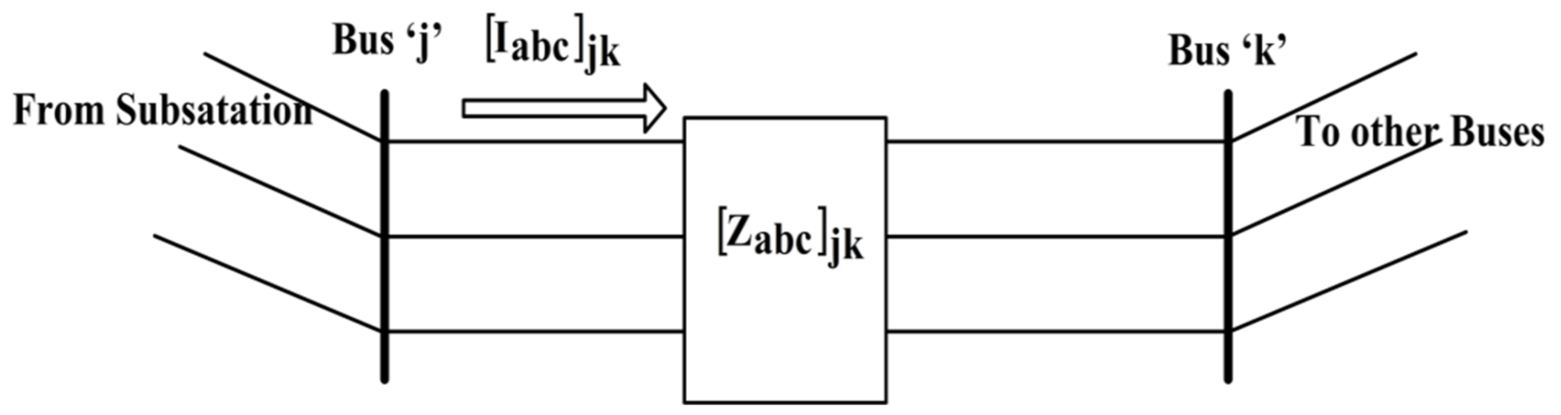
With the Carson’s equations presented in [23], the primitive impedance matrices for three-phase overhead and underground lines can be formed. For a grounded neural system, these matrices are reduced to phase impedance matrices of $3\times 3$ size using Kron reduction. Figure 1 shows the three-phase distribution line model, and its shunt admittance is neglected due to its small effect. The phase impedance matrix for the line section ‘jk’ is given in Equation (1).

$${\left[{\mathrm{Z}}_{\mathrm{a}\mathrm{b}\mathrm{c}}\right]}_{\mathrm{j}\mathrm{k}}={\left[\begin{array}{ccc}{\mathrm{Z}}_{\mathrm{a}\mathrm{a}}& {\mathrm{Z}}_{\mathrm{a}\mathrm{b}}& {\mathrm{Z}}_{\mathrm{a}\mathrm{c}}\\ {\mathrm{Z}}_{\mathrm{b}\mathrm{a}}& {\mathrm{Z}}_{\mathrm{b}\mathrm{b}}& {\mathrm{Z}}_{\mathrm{b}\mathrm{c}}\\ {\mathrm{Z}}_{\mathrm{c}\mathrm{a}}& {\mathrm{Z}}_{\mathrm{c}\mathrm{b}}& {\mathrm{Z}}_{\mathrm{c}\mathrm{c}}\end{array}\right]}_{\mathrm{j}\mathrm{k}}$$

(1)

Figure 1. A sample three-phase distribution line.

From Figure 1, the relationship between the phase voltage matrices of bus-j and bus-k is given in Equation (2):

$${\left[\begin{array}{c}{\mathrm{V}}_{\mathrm{a}}\\ {\mathrm{V}}_{\mathrm{b}}\\ {\mathrm{V}}_{\mathrm{c}}\end{array}\right]}_{\mathrm{k}}={\left[\begin{array}{c}{\mathrm{V}}_{\mathrm{a}}\\ {\mathrm{V}}_{\mathrm{b}}\\ {\mathrm{V}}_{\mathrm{c}}\end{array}\right]}_{\mathrm{j}}-{\left[\begin{array}{ccc}{\mathrm{Z}}_{\mathrm{a}\mathrm{a}}& {\mathrm{Z}}_{\mathrm{a}\mathrm{b}}& {\mathrm{Z}}_{\mathrm{a}\mathrm{c}}\\ {\mathrm{Z}}_{\mathrm{b}\mathrm{a}}& {\mathrm{Z}}_{\mathrm{b}\mathrm{b}}& {\mathrm{Z}}_{\mathrm{b}\mathrm{c}}\\ {\mathrm{Z}}_{\mathrm{c}\mathrm{a}}& {\mathrm{Z}}_{\mathrm{c}\mathrm{b}}& {\mathrm{Z}}_{\mathrm{c}\mathrm{c}}\end{array}\right]}_{\mathrm{j}\mathrm{k}}\cdot {\left[\begin{array}{c}{\mathrm{I}}_{\mathrm{a}}\\ {\mathrm{I}}_{\mathrm{b}}\\ {\mathrm{I}}_{\mathrm{c}}\end{array}\right]}_{\mathrm{j}\mathrm{k}}$$

(2)

The reactance of line is regarded as proportionate to the harmonic order for HPFA. For h-order harmonic frequency, the self-impedance of phase ‘a’ is given in Equation (3),

$${\left({\mathrm{Z}}_{\mathrm{a}\mathrm{a}}\right)}^{\mathrm{h}}={\mathrm{R}}_{\mathrm{a}\mathrm{a}}+\mathrm{j}\cdot \mathrm{h}\cdot {\mathrm{X}}_{\mathrm{a}\mathrm{a}}$$

(3)

2.2. Loads

The phase current matrix and line current matrix serving the different types of three-phase loads are outlined in Table 1. Detailed discussion on Table 1 is provided in [23].

Table 1. Load modelling.

	Wye Connection	Delta Connection
Phase voltage matrix and specified load matrix at bus.	$\left[\begin{array}{c}\left|{\mathrm{V}}_{\mathrm{a}\mathrm{n}}\right|\angle {\delta }_{\mathrm{a}}\\ \left|{\mathrm{V}}_{\mathrm{b}\mathrm{n}}\right|\angle {\delta }_{\mathrm{b}}\\ \left|{\mathrm{V}}_{\mathrm{c}\mathrm{n}}\right|\angle {\delta }_{\mathrm{c}}\end{array}\right]$, $\left[\begin{array}{c}\left|{\mathrm{S}}_{\mathrm{a}}\right|\angle {\mathsf{\theta }}_{\mathrm{a}}\\ \left|{\mathrm{S}}_{\mathrm{b}}\right|\angle {\mathsf{\theta }}_{\mathrm{b}}\\ \left|{\mathrm{S}}_{\mathrm{c}}\right|\angle {\mathsf{\theta }}_{\mathrm{c}}\end{array}\right]$	$\left[\begin{array}{c}\left|{\mathrm{V}}_{\mathrm{a}\mathrm{b}}\right|\angle {\delta }_{\mathrm{a}\mathrm{b}}\\ \left|{\mathrm{V}}_{\mathrm{b}\mathrm{c}}\right|\angle {\delta }_{\mathrm{b}\mathrm{c}}\\ \left|{\mathrm{V}}_{\mathrm{c}\mathrm{a}}\right|\angle {\delta }_{\mathrm{c}\mathrm{a}}\end{array}\right]$, $\left[\begin{array}{c}\left|{\mathrm{S}}_{\mathrm{a}\mathrm{b}}\right|\angle {\mathsf{\theta }}_{\mathrm{a}\mathrm{b}}\\ \left|{\mathrm{S}}_{\mathrm{b}\mathrm{c}}\right|\angle {\mathsf{\theta }}_{\mathrm{b}\mathrm{c}}\\ \left|{\mathrm{S}}_{\mathrm{c}\mathrm{a}}\right|\angle {\mathsf{\theta }}_{\mathrm{c}\mathrm{a}}\end{array}\right]$
Phase current matrix serving constant power load	$\left[\begin{array}{c}\mathrm{I}{\mathrm{L}}_{\mathrm{a}}\\ \mathrm{I}{\mathrm{L}}_{\mathrm{b}}\\ \mathrm{I}{\mathrm{L}}_{\mathrm{c}}\end{array}\right]=\left[\begin{array}{c}{\left(\frac{{\mathrm{S}}_{\mathrm{a}}}{{\mathrm{V}}_{\mathrm{a}\mathrm{n}}}\right)}^{\ast }\\ {\left(\frac{{\mathrm{S}}_{\mathrm{b}}}{{\mathrm{V}}_{\mathrm{b}\mathrm{n}}}\right)}^{\ast }\\ {\left(\frac{{\mathrm{S}}_{\mathrm{c}}}{{\mathrm{V}}_{\mathrm{c}\mathrm{n}}}\right)}^{\ast }\end{array}\right]$	$\left[\begin{array}{c}\mathrm{I}{\mathrm{L}}_{\mathrm{a}\mathrm{b}}\\ \mathrm{I}{\mathrm{L}}_{\mathrm{b}\mathrm{c}}\\ \mathrm{I}{\mathrm{L}}_{\mathrm{c}\mathrm{a}}\end{array}\right]=\left[\begin{array}{c}{\left(\frac{{\mathrm{S}}_{\mathrm{a}\mathrm{b}}}{{\mathrm{V}}_{\mathrm{a}\mathrm{b}}}\right)}^{\ast }\\ {\left(\frac{{\mathrm{S}}_{\mathrm{b}\mathrm{c}}}{{\mathrm{V}}_{\mathrm{b}\mathrm{c}}}\right)}^{\ast }\\ {\left(\frac{{\mathrm{S}}_{\mathrm{c}\mathrm{a}}}{{\mathrm{V}}_{\mathrm{c}\mathrm{a}}}\right)}^{\ast }\end{array}\right]$
Phase current matrix serving the constant impedance load	$\left[\begin{array}{c}\mathrm{Z}{\mathrm{L}}_{\mathrm{a}}\\ \mathrm{Z}{\mathrm{L}}_{\mathrm{b}}\\ \mathrm{Z}{\mathrm{L}}_{\mathrm{c}}\end{array}\right]=\left[\begin{array}{c}\frac{{\left|{\mathrm{V}}_{\mathrm{a}\mathrm{n}}\right|}^2}{{\mathrm{S}}_{\mathrm{a}}^{\ast }}\\ \frac{{\left|{\mathrm{V}}_{\mathrm{b}\mathrm{n}}\right|}^2}{{\mathrm{S}}_{\mathrm{b}}^{\ast }}\\ \frac{{\left|{\mathrm{V}}_{\mathrm{c}\mathrm{n}}\right|}^2}{{\mathrm{S}}_{\mathrm{c}}^{\ast }}\end{array}\right]$ $\left[\begin{array}{c}\mathrm{I}{\mathrm{L}}_{\mathrm{a}}\\ \mathrm{I}{\mathrm{L}}_{\mathrm{b}}\\ \mathrm{I}{\mathrm{L}}_{\mathrm{c}}\end{array}\right]=\left[\begin{array}{c}\frac{{\mathrm{V}}_{\mathrm{a}\mathrm{n}}}{\mathrm{Z}{\mathrm{L}}_{\mathrm{a}}}\\ \frac{{\mathrm{V}}_{\mathrm{b}\mathrm{n}}}{\mathrm{Z}{\mathrm{L}}_{\mathrm{b}}}\\ \frac{{\mathrm{V}}_{\mathrm{c}\mathrm{n}}}{\mathrm{Z}{\mathrm{L}}_{\mathrm{c}}}\end{array}\right]$	$\left[\begin{array}{c}\mathrm{Z}{\mathrm{L}}_{\mathrm{a}\mathrm{b}}\\ \mathrm{Z}{\mathrm{L}}_{\mathrm{b}\mathrm{c}}\\ \mathrm{Z}{\mathrm{L}}_{\mathrm{c}\mathrm{a}}\end{array}\right]=\left[\begin{array}{c}\frac{{\left|{\mathrm{V}}_{\mathrm{a}\mathrm{b}}\right|}^2}{{\mathrm{S}}_{\mathrm{a}\mathrm{b}}^{\ast }}\\ \frac{{\left|{\mathrm{V}}_{\mathrm{b}\mathrm{c}}\right|}^2}{{\mathrm{S}}_{\mathrm{b}\mathrm{c}}^{\ast }}\\ \frac{{\left|{\mathrm{V}}_{\mathrm{c}\mathrm{a}}\right|}^2}{{\mathrm{S}}_{\mathrm{c}\mathrm{a}}^{\ast }}\end{array}\right]$ $\left[\begin{array}{c}\mathrm{I}{\mathrm{L}}_{\mathrm{a}\mathrm{b}}\\ \mathrm{I}{\mathrm{L}}_{\mathrm{b}\mathrm{c}}\\ \mathrm{I}{\mathrm{L}}_{\mathrm{c}\mathrm{a}}\end{array}\right]=\left[\begin{array}{c}\frac{{\mathrm{V}}_{\mathrm{a}\mathrm{b}}}{\mathrm{Z}{\mathrm{L}}_{\mathrm{a}\mathrm{b}}}\\ \frac{{\mathrm{V}}_{\mathrm{b}\mathrm{c}}}{\mathrm{Z}{\mathrm{L}}_{\mathrm{b}\mathrm{c}}}\\ \frac{{\mathrm{V}}_{\mathrm{c}\mathrm{a}}}{\mathrm{Z}{\mathrm{L}}_{\mathrm{c}\mathrm{a}}}\end{array}\right]$
Phase current matrix serving the constant current load	$\left[\begin{array}{c}\mathrm{I}{\mathrm{L}}_{\mathrm{a}}\\ \mathrm{I}{\mathrm{L}}_{\mathrm{b}}\\ \mathrm{I}{\mathrm{L}}_{\mathrm{c}}\end{array}\right]=\left[\begin{array}{c}\left|\mathrm{I}{\mathrm{L}}_{\mathrm{a}}\right|\angle \left({\delta }_{\mathrm{a}}-{\mathsf{\theta }}_{\mathrm{a}}\right)\\ \left|\mathrm{I}{\mathrm{L}}_{\mathrm{b}}\right|\angle \left({\delta }_{\mathrm{b}}-{\mathsf{\theta }}_{\mathrm{b}}\right)\\ \left|\mathrm{I}{\mathrm{L}}_{\mathrm{c}}\right|\angle \left({\delta }_{\mathrm{c}}-{\mathsf{\theta }}_{\mathrm{c}}\right)\end{array}\right]$	$\left[\begin{array}{c}\mathrm{I}{\mathrm{L}}_{\mathrm{a}\mathrm{b}}\\ \mathrm{I}{\mathrm{L}}_{\mathrm{b}\mathrm{c}}\\ \mathrm{I}{\mathrm{L}}_{\mathrm{c}\mathrm{a}}\end{array}\right]=\left[\begin{array}{c}\left|\mathrm{I}{\mathrm{L}}_{\mathrm{a}\mathrm{b}}\right|\angle \left({\delta }_{\mathrm{a}\mathrm{b}}-{\mathsf{\theta }}_{\mathrm{a}\mathrm{b}}\right)\\ \left|\mathrm{I}{\mathrm{L}}_{\mathrm{b}\mathrm{c}}\right|\angle \left({\delta }_{\mathrm{b}\mathrm{c}}-{\mathsf{\theta }}_{\mathrm{b}\mathrm{c}}\right)\\ \left|\mathrm{I}{\mathrm{L}}_{\mathrm{c}\mathrm{a}}\right|\angle \left({\delta }_{\mathrm{c}\mathrm{a}}-{\mathsf{\theta }}_{\mathrm{c}\mathrm{a}}\right)\end{array}\right]$
Line current matrix entering the load	$\left[\begin{array}{c}\mathrm{I}{\mathrm{L}}_{\mathrm{a}}\\ \mathrm{I}{\mathrm{L}}_{\mathrm{b}}\\ \mathrm{I}{\mathrm{L}}_{\mathrm{c}}\end{array}\right]$	$\left[\begin{array}{c}\mathrm{I}{\mathrm{L}}_{\mathrm{a}}\\ \mathrm{I}{\mathrm{L}}_{\mathrm{b}}\\ \mathrm{I}{\mathrm{L}}_{\mathrm{c}}\end{array}\right]=\left[\begin{array}{ccc}1& 0& -1\\ -1& 1& 0\\ 0& -1& 1\end{array}\right]\cdot \left[\begin{array}{c}\mathrm{I}{\mathrm{L}}_{\mathrm{a}\mathrm{b}}\\ \mathrm{I}{\mathrm{L}}_{\mathrm{b}\mathrm{c}}\\ \mathrm{I}{\mathrm{L}}_{\mathrm{c}\mathrm{a}}\end{array}\right]$
Distributed Loads	Create a duplicate node at a distance of one-fourth the length from the sending end and connect a two-third of lode. At the receiving end one-third of load is connected.

2.2.1. Linear Loads

These loads produce only fundamental sinusoidal response upon supplied by sinusoidal source. The liner loads can be modelled in several ways [1]. Each model will show a different impact on harmonic analysis. The impedance modelling of these loads is taken as series combination of R and X.

2.2.2. Non-Linear Loads

With the harmonic spectrum of non-linear loads and their load current obtained from the fundamental power flow, these loads are modelled as constant current sources [24]. The magnitude of the current source is obtained with Equation (4), and its phase angle is obtained with Equation (5):

$${\mathrm{I}}_{\mathrm{h}}={\mathrm{I}}_{\mathrm{r}\mathrm{a}\mathrm{t}\mathrm{e}\mathrm{d}}\frac{{\mathrm{I}}_{\mathrm{h}\_\mathrm{s}\mathrm{p}\mathrm{e}\mathrm{c}\mathrm{t}\mathrm{r}\mathrm{u}\mathrm{m}}}{{\mathrm{I}}_{1\_\mathrm{s}\mathrm{p}\mathrm{e}\mathrm{c}\mathrm{t}\mathrm{r}\mathrm{u}\mathrm{m}}}$$

(4)

The phase angle of the current source is obtained as:

$${\mathsf{\theta }}_{\mathrm{h}}={\mathsf{\theta }}_{\mathrm{h}\_\mathrm{s}\mathrm{p}\mathrm{e}\mathrm{c}\mathrm{t}\mathrm{r}\mathrm{u}\mathrm{m}}+\mathrm{h}\left({\mathsf{\theta }}_1-{\mathsf{\theta }}_{\mathrm{h}\_\mathrm{s}\mathrm{p}\mathrm{e}\mathrm{t}\mathrm{r}\mathrm{u}\mathrm{m}}\right)$$

(5)

where:

${\mathsf{\theta }}_1:$ Phase angle of the rated current at fundamental frequency;

${\mathsf{\theta }}_{\mathrm{h}\_\mathrm{s}\mathrm{p}\mathrm{e}\mathrm{c}\mathrm{t}\mathrm{r}\mathrm{u}\mathrm{m}}:$ Phase angle of the harmonic source current spectrum.

2.3. Capacitor Banks

Modelling of the capacitor banks is presented in Table 2.

Table 2. Capacitor banks modeling.

	Wye Connected	Delta Connected
Phase voltage matrix and specified reactive power matrix at bus.	$\left[\begin{array}{c}\left|{\mathrm{V}}_{\mathrm{a}\mathrm{n}}\right|\angle {\mathsf{\theta }}_{\mathrm{a}}\\ \left|{\mathrm{V}}_{\mathrm{b}\mathrm{n}}\right|\angle {\mathsf{\theta }}_{\mathrm{b}}\\ \left|{\mathrm{V}}_{\mathrm{c}\mathrm{n}}\right|\angle {\mathsf{\theta }}_{\mathrm{c}}\end{array}\right]$, $\left[\begin{array}{c}{\mathrm{Q}}_{\mathrm{a}}\\ {\mathrm{Q}}_{\mathrm{b}}\\ {\mathrm{Q}}_{\mathrm{c}}\end{array}\right]$	$\left[\begin{array}{c}\left|{\mathrm{V}}_{\mathrm{a}\mathrm{b}}\right|\angle {\mathsf{\theta }}_{\mathrm{a}\mathrm{b}}\\ \left|{\mathrm{V}}_{\mathrm{b}\mathrm{c}}\right|\angle {\mathsf{\theta }}_{\mathrm{b}\mathrm{c}}\\ \left|{\mathrm{V}}_{\mathrm{c}\mathrm{a}}\right|\angle {\mathsf{\theta }}_{\mathrm{c}\mathrm{a}}\end{array}\right]$,$\left[\begin{array}{c}{\mathrm{Q}}_{\mathrm{a}\mathrm{b}}\\ {\mathrm{Q}}_{\mathrm{b}\mathrm{c}}\\ {\mathrm{Q}}_{\mathrm{c}\mathrm{a}}\end{array}\right]$
Phase current matrix serving the capacitor bank	$\left[{\mathrm{B}}_{\mathrm{a}\mathrm{b}\mathrm{c}}\right]=\left[\begin{array}{c}\frac{{\mathrm{Q}}_{\mathrm{a}}}{{\left|{\mathrm{V}}_{\mathrm{a}}\right|}^2}\\ \frac{{\mathrm{Q}}_{\mathrm{b}}}{{\left|{\mathrm{V}}_{\mathrm{b}}\right|}^2}\\ \frac{{\mathrm{Q}}_{\mathrm{c}}}{{\left|{\mathrm{V}}_{\mathrm{c}}\right|}^2}\end{array}\right]$ $\left[\begin{array}{c}\mathrm{I}{\mathrm{C}}_{\mathrm{a}}\\ \mathrm{I}{\mathrm{C}}_{\mathrm{b}}\\ \mathrm{I}{\mathrm{C}}_{\mathrm{c}}\end{array}\right]=\left[\begin{array}{c}\mathrm{j}\cdot {\mathrm{B}}_{\mathrm{a}}\cdot {\mathrm{V}}_{\mathrm{a}\mathrm{n}}\\ \mathrm{j}\cdot {\mathrm{B}}_{\mathrm{b}}\cdot {\mathrm{V}}_{\mathrm{b}\mathrm{n}}\\ \mathrm{j}\cdot {\mathrm{B}}_{\mathrm{c}}\cdot {\mathrm{V}}_{\mathrm{c}\mathrm{n}}\end{array}\right]$	$\left[{\mathrm{B}}_{\mathrm{a}\mathrm{b}\mathrm{c}}\right]=\left[\begin{array}{c}\frac{{\mathrm{Q}}_{\mathrm{a}\mathrm{b}}}{{\left|{\mathrm{V}}_{\mathrm{a}\mathrm{b}}\right|}^2}\\ \frac{{\mathrm{Q}}_{\mathrm{b}\mathrm{c}}}{{\left|{\mathrm{V}}_{\mathrm{b}\mathrm{c}}\right|}^2}\\ \frac{{\mathrm{Q}}_{\mathrm{c}\mathrm{a}}}{{\left|{\mathrm{V}}_{\mathrm{c}\mathrm{a}}\right|}^2}\end{array}\right]$ $\left[\begin{array}{c}\mathrm{I}{\mathrm{C}}_{\mathrm{a}\mathrm{b}}\\ \mathrm{I}{\mathrm{C}}_{\mathrm{b}\mathrm{c}}\\ \mathrm{I}{\mathrm{C}}_{\mathrm{c}\mathrm{a}}\end{array}\right]=\left[\begin{array}{c}\mathrm{j}\cdot {\mathrm{B}}_{\mathrm{a}\mathrm{b}}\cdot {\mathrm{V}}_{\mathrm{a}\mathrm{b}}\\ \mathrm{j}\cdot {\mathrm{B}}_{\mathrm{b}\mathrm{c}}\cdot {\mathrm{V}}_{\mathrm{b}\mathrm{c}}\\ \mathrm{j}\cdot {\mathrm{B}}_{\mathrm{c}\mathrm{a}}\cdot {\mathrm{V}}_{\mathrm{c}\mathrm{a}}\end{array}\right]$
Line current matrix serving the capacitor bank	$\left[\begin{array}{c}\mathrm{I}{\mathrm{C}}_{\mathrm{a}}\\ \mathrm{I}{\mathrm{C}}_{\mathrm{b}}\\ \mathrm{I}{\mathrm{C}}_{\mathrm{c}}\end{array}\right]$	$\left[\begin{array}{c}\mathrm{I}{\mathrm{C}}_{\mathrm{a}}\\ \mathrm{I}{\mathrm{C}}_{\mathrm{b}}\\ \mathrm{I}{\mathrm{C}}_{\mathrm{c}}\end{array}\right]=\left[\begin{array}{ccc}1& 0& -1\\ -1& 1& 0\\ 0& -1& 1\end{array}\right]\cdot \left[\begin{array}{c}\mathrm{I}{\mathrm{C}}_{\mathrm{a}\mathrm{b}}\\ \mathrm{I}{\mathrm{C}}_{\mathrm{b}\mathrm{c}}\\ \mathrm{I}{\mathrm{C}}_{\mathrm{c}\mathrm{a}}\end{array}\right]$

For HPFA, the capacitive susceptance (B) is to be multiplied with ‘h’ for ‘h’ order frequency.

2.4. Tree-Phase Transformer

The fundamental voltage and current relationships between the primary and secondary sides for different transformer connections are presented in [25]. The modelling of the three-phase transformers for HPFA is given in [24,26].

2.5. D-STATCOM

The D-STATCOM is commonly regarded as a shunt compensator which supplies reactive power in PFAs. The voltage magnitude at the D-STATCOM bus can be controlled by adjusting the reactive power injection of D-STATCOM.

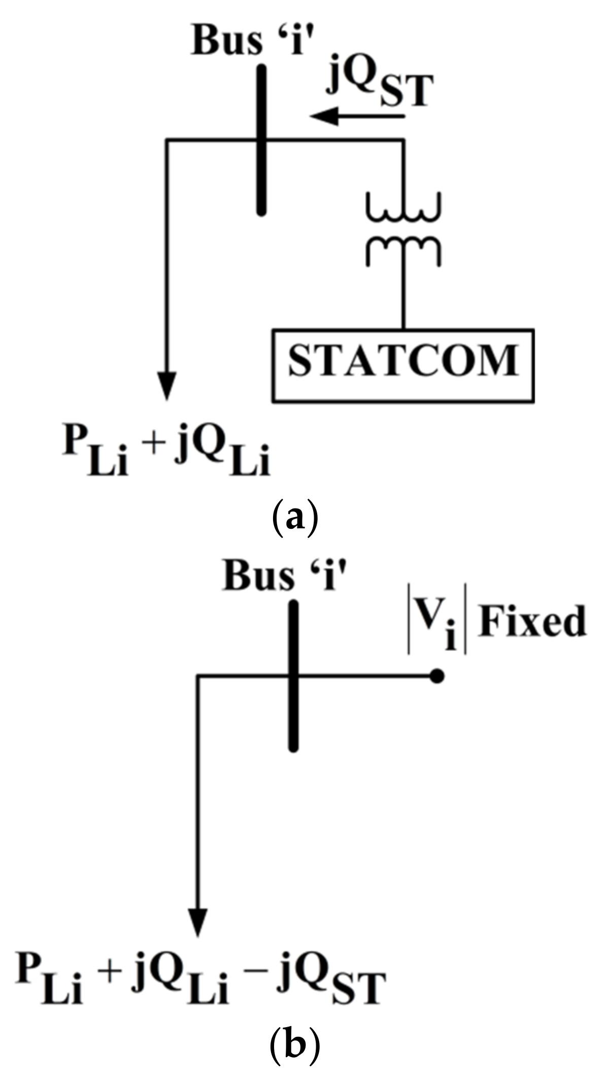
The interface of the D-STATCOM at i^th bus shown in Figure 2a, and its traditional modelling for PFAs is shown in Figure 2b. The specified reactive power of the load is combined with the reactive power output of D-STATCOM, so that reactive power varies as magnitude of V_i varies. This is absolutely a PV bus modelling with the real power output of the D-STATCOM set to zero [27,28]. The hypothesis in this model is that losses in the D-STATCOM and its connection are ignored. The D-STATCOMs have low harmonic content, so the harmonic current injected by the D-STATCOM is considered as zero for HPFA.

Figure 2. (a) D-STATCOM interface at i^th bus 2 (b) Traditional modelling of D-STATCOM as PV bus.

3. Algorithm for Developing BNM and BRNM

The performance of the HPFA of URDN is enhanced by the systematic numbering of buses and branches. From [29], the numbering scheme to buses and branches is taken. The following steps are to be followed to write a Software Code in order to split the URDN into different sections, as shown in Figure 3.

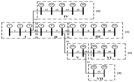
Figure 3. Divided sections for sample distribution network.

• From the distribution network shown in Figure 3, form Table 3.
  Table 3. Branch numbering of distribution network in Figure 2.

  Branch Number(BN)	Sending Bus(SE)	Receiving Bus(RE)
  1	1	2
  2	2	3
  3	3	4
  4	4	5
  5	5	6
  6	6	7
  7	7	8
  8	8	9
  9	9	10
  10	10	11
  11	3	12
  12	12	13
  13	13	14
  14	14	15
  15	15	16
  16	6	17
  17	17	18
  18	18	19
  19	19	20
  20	20	21
  21	18	22
  22	22	23

• Start with BN = 1.Read the RE of BN, i.e., 2. Then, check how many times this 2 appears in the SE row. Inthe above table, it appears one time. That means bus 2 is the sending end for only one branch. Fill these RE 2 and BN 1 in two different matrices (BNM and BRNM) as the first row and first column elements. Then, increase the column number by one.
• Increase the BN (i.e., BN = 2), and read the RE of BN, i.e., 3. Then, as in step 1, check for the appearance of 3 in SE row. The bus 3 appears two times. That means that, from the bus 3, two branches are leaving. Then, fill these RE 3 and BN 2 into the same variables as the first row and present the column elements. Name this row elements as section-I. Now increase the row number by one and set the column number to one.
• Similarly, increase the BN, and read the RE of BN. Then, check for the appearance of this RE in the SE row. If it appears one time, then fill these RE and BN values as the present row and present column elements of the variables BNM and BRNM. Then increase the column number by one and repeat step 4. If it does not appears or appears more than one time in the SE row, then fill the corresponding RE and BN values as present row and present column elements. Then identify this row as a section. Then increase the row number by one and set the column number to one and repeat the step 4.

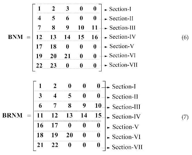
The above steps are repeated until the BN value reaches the last branch number. At the end, the BNM and BRNM are obtained as follows:

4. Three-Phase HPFA with Non-Linear Loads and D-STATCOM Devices

For modeling the linear and non-linear loads for HPFA, the fundamental power flow solution is required. Hence, the algorithm consists of two parts. PartA illustrates the iterative procedure for FPFA with the D-STATCOM device and PartB illustrates the iterative procedure for HPFA with linear loads, non-linear loads, and D-STATCOM devices.

After developing the BNM and BRNM for the URDN, the iterative procedure is explained with the following steps.

PartA: FPFA with D-STATCOM

• The voltages at all busses are assigned as substation bus voltage.

  $$\left[\begin{array}{c}{\mathrm{V}}_{\mathrm{a}}\\ {\mathrm{V}}_{\mathrm{b}}\\ {\mathrm{V}}_{\mathrm{c}}\end{array}\right]=\left[\begin{array}{c}1\angle 0^{\mathrm{o}}\\ 1\angle -{120}^{\mathrm{o}}\\ 1\angle {120}^{\mathrm{o}}\end{array}\right]$$

  (8)
• Find the line current matrix serving the load at all buses.
• Start with collecting line current matrix at bus−23 (the tail bus in section-VII in BNM), and thereby find the line current matrix for branch−22 (the tail branch in section-VII in BRNM). Then, continue to the bus−22 and branch−21 to find the line current matrix at the bus and line current matrix in branch, respectively. From Figure 4, the following equations are obtained by applying the KCL at every bus:

  $${\left[{\mathrm{I}}_{\mathrm{a}\mathrm{b}\mathrm{c}}\right]}_{\mathrm{k}}={\left[\mathrm{I}{\mathrm{L}}_{\mathrm{a}\mathrm{b}\mathrm{c}}\right]}_{\mathrm{k}}+{\left[\mathrm{I}\mathrm{s}{\mathrm{h}}_{\mathrm{a}\mathrm{b}\mathrm{c}}\right]}_{\mathrm{k}}+{\left[\mathrm{I}{\mathrm{C}}_{\mathrm{a}\mathrm{b}\mathrm{c}}\right]}_{\mathrm{k}}$$

  (9)

  $${\left[{\mathrm{I}}_{\mathrm{a}\mathrm{b}\mathrm{c}}\right]}_{\mathrm{j}\mathrm{k}}={\left[{\mathrm{I}}_{\mathrm{a}\mathrm{b}\mathrm{c}}\right]}_{\mathrm{k}}$$

  (10)

  $${\left[{\mathrm{I}}_{\mathrm{a}\mathrm{b}\mathrm{c}}\right]}_{\mathrm{j}}={\left[{\mathrm{I}}_{\mathrm{a}\mathrm{b}\mathrm{c}}\right]}_{\mathrm{j}\mathrm{k}}+{\left[\mathrm{I}{\mathrm{L}}_{\mathrm{a}\mathrm{b}\mathrm{c}}\right]}_{\mathrm{j}}+{\left[\mathrm{I}\mathrm{s}{\mathrm{h}}_{\mathrm{a}\mathrm{b}\mathrm{c}}\right]}_{\mathrm{j}}+{\left[\mathrm{I}{\mathrm{C}}_{\mathrm{a}\mathrm{b}\mathrm{c}}\right]}_{\mathrm{j}}$$

  (11)

  $${\left[{\mathrm{I}}_{\mathrm{a}\mathrm{b}\mathrm{c}}\right]}_{\mathrm{i}\mathrm{j}}={\left[{\mathrm{I}}_{\mathrm{a}\mathrm{b}\mathrm{c}}\right]}_{\mathrm{j}}$$

  (12)

  $${\left[{\mathrm{I}}_{\mathrm{a}\mathrm{b}\mathrm{c}}\right]}_{\mathrm{i}}={\left[{\mathrm{I}}_{\mathrm{a}\mathrm{b}\mathrm{c}}\right]}_{\mathrm{i}\mathrm{j}}$$

  (13)

  where:
  

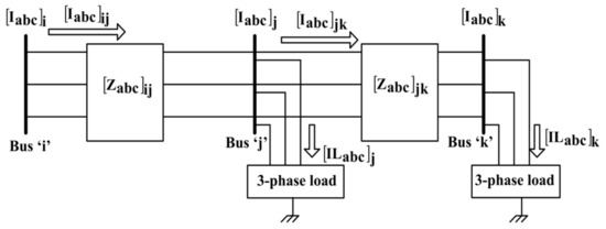  Figure 4. A simple URDN three busses.
  ${\left[{\mathrm{I}}_{\mathrm{a}\mathrm{b}\mathrm{c}}\right]}_{\mathrm{k}}:$ Line current matrix at bus-k;
  ${\left[\mathrm{I}{\mathrm{L}}_{\mathrm{a}\mathrm{b}\mathrm{c}}\right]}_{\mathrm{j}\mathrm{k}}:$ Line current in branch-jk;
  ${\left[\mathrm{I}{\mathrm{L}}_{\mathrm{a}\mathrm{b}\mathrm{c}}\right]}_{\mathrm{k}}:$ Load current matrix at bus-k;
  ${\left[\mathrm{I}\mathrm{s}{\mathrm{h}}_{\mathrm{a}\mathrm{b}\mathrm{c}}\right]}_{\mathrm{k}}:$ Line current matrix drawn by shunt admittance at bus-k;
  ${\left[\mathrm{I}{\mathrm{C}}_{\mathrm{a}\mathrm{b}\mathrm{c}}\right]}_{\mathrm{k}}:$ Line current matrix drawn by capacitor bank at bus-k, if any.
• Now go to section-VI and repeat procedure as in step 5 to find the line current matrix at the head bus and line current matrix for head branch. Similarly, proceed up to section-I and find the line current matrix up to bus−1 and line current matrix up to branch−1.
• Now start with head bus in section-I and continue to the tail bus in section-I by finding the phase voltage matrix at all buses with Equation (2). Then, go to the next section and repeat the same procedure.
• Steps 4 to 6 are to be repeated until the convergence criterion as given in Equation (14) is satisfied:

  $$\left|{\left[{\mathrm{V}}_{\mathrm{a}\mathrm{b}\mathrm{c}}\right]}_{\mathrm{i}}^{\mathrm{r}}-{\left[{\mathrm{V}}_{\mathrm{a}\mathrm{b}\mathrm{c}}\right]}_{\mathrm{i}}^{\mathrm{r}-1}\right|\le \left[{\mathsf{\epsilon }}_{\mathrm{a}\mathrm{b}\mathrm{c}}\right]$$

  (14)

  where ‘r’ is the iteration number.
• D-STATCOM location is selected and model as PV bus for the outside γ^thiteration.
• The mismatches in voltages at D-STATCOM buses are obtained with Equation (13):

  $${\left[\begin{array}{c}\Delta {\mathrm{V}}_{\mathrm{a}}\\ \Delta {\mathrm{V}}_{\mathrm{b}}\\ \Delta {\mathrm{V}}_{\mathrm{c}}\end{array}\right]}_{}^{\gamma }=\left|\begin{array}{c}{\mathrm{V}}_{\mathrm{a}}^{\mathrm{s}\mathrm{p}}\\ {\mathrm{V}}_{\mathrm{b}}^{\mathrm{s}\mathrm{p}}\\ {\mathrm{V}}_{\mathrm{c}}^{\mathrm{s}\mathrm{p}}\end{array}\right|-{\left|\begin{array}{c}{\mathrm{V}}_{\mathrm{a}}^{\mathrm{c}\mathrm{a}\mathrm{l}}\\ {\mathrm{V}}_{\mathrm{b}}^{\mathrm{c}\mathrm{a}\mathrm{l}}\\ {\mathrm{V}}_{\mathrm{c}}^{\mathrm{c}\mathrm{a}\mathrm{l}}\end{array}\right|}^{\gamma }$$

  (15)

  $${\left[\Delta {\mathrm{V}}_{\mathrm{a}\mathrm{b}\mathrm{c}}\right]}^{\gamma }\le \left[{\mathsf{\epsilon }}_{\mathrm{a}\mathrm{b}\mathrm{c}}\right]$$

  (16)

  where ${\left[\Delta \mathrm{V}\right]}^{\gamma }$ is the mismatch matrix for the voltage and its size is $3\cdot \mathrm{n}\times 1$, and ‘n’ is the total number of PV buses.
• If the Equation (16) is not satisfied, then the incremental current injection matrix at D-STATCOM bus is calculated with Equation (17) to maintain the specified voltages:

  $${\left[\Delta \mathrm{I}\right]}^{\gamma }={\left[{\mathrm{Z}}_{\mathrm{P}\mathrm{V}}\right]}^{-1}\cdot {\left[\Delta \mathrm{V}\right]}^{\gamma }$$

  (17)

  where $\left[{\mathrm{Z}}_{\mathrm{P}\mathrm{V}}\right]$ is the sensitivity matrix for the PV bus with its size $3\cdot \mathrm{n}\times 3\cdot \mathrm{n}$. The formation of this matrix is presented in [30].
• The incremental reactive current injection matrix at D-STATCOM bus is obtained with Equation (18):

  $${\left[\begin{array}{c}\Delta {\mathrm{I}}_{\mathrm{D},\mathrm{a}}\\ \Delta {\mathrm{I}}_{\mathrm{D},\mathrm{b}}\\ \Delta {\mathrm{I}}_{\mathrm{D},\mathrm{c}}\end{array}\right]}_{\mathrm{j}}^{\gamma }={\left[\begin{array}{c}\left|\Delta {\mathrm{I}}_{\mathrm{a}}\right|\cdot \left(\mathrm{c}\mathrm{o}\mathrm{s}\left(90^0+{\delta }_{\mathrm{v},\mathrm{a}}\right)+\mathrm{j}*\mathrm{s}\mathrm{i}\mathrm{n}\left(90^0+{\delta }_{\mathrm{v},\mathrm{a}}\right)\right)\\ \left|\Delta {\mathrm{I}}_{\mathrm{b}}\right|\cdot \left(\mathrm{c}\mathrm{o}\mathrm{s}\left(90^0+{\delta }_{\mathrm{v},\mathrm{b}}\right)+\mathrm{j}*\mathrm{s}\mathrm{i}\mathrm{n}\left(90^0+{\delta }_{\mathrm{v},\mathrm{b}}\right)\right)\\ \left|\Delta {\mathrm{I}}_{\mathrm{c}}\right|\cdot \left(\mathrm{c}\mathrm{o}\mathrm{s}\left(90^0+{\delta }_{\mathrm{v},\mathrm{c}}\right)+\mathrm{j}*\mathrm{s}\mathrm{i}\mathrm{n}\left(90^0+{\delta }_{\mathrm{v},\mathrm{c}}\right)\right)\end{array}\right]}_{\mathrm{j}}^{\gamma }$$

  (18)
• In Figure 5, by applying the KCL at bus-j, the line current matrix in branch-ij is obtained as:

  $${\left[\begin{array}{c}{\mathrm{I}}_{\mathrm{a}}\\ {\mathrm{I}}_{\mathrm{b}}\\ {\mathrm{I}}_{\mathrm{c}}\end{array}\right]}_{\mathrm{i}\mathrm{j}}^{\gamma }={\left[\begin{array}{c}\mathrm{I}{\mathrm{L}}_{\mathrm{a}}\\ \mathrm{I}{\mathrm{L}}_{\mathrm{b}}\\ \mathrm{I}{\mathrm{L}}_{\mathrm{c}}\end{array}\right]}_{\mathrm{j}}^{\gamma }-{\left[\begin{array}{c}\Delta {\mathrm{I}}_{\mathrm{D},\mathrm{a}}\\ \Delta {\mathrm{I}}_{\mathrm{D},\mathrm{b}}\\ \Delta {\mathrm{I}}_{\mathrm{D},\mathrm{c}}\end{array}\right]}_{\mathrm{j}}^{\gamma }$$

  (19)
  

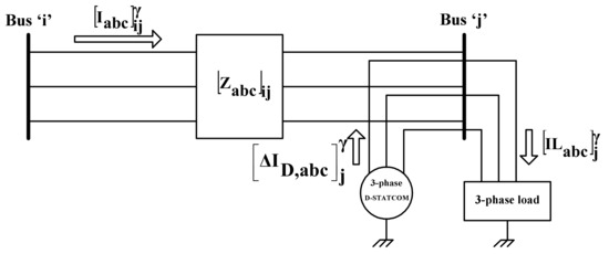  Figure 5. A simple URDN with two buses with D-STATCOM placed at bus-j.
  With ${\left[{\mathrm{V}}_{\mathrm{a}\mathrm{b}\mathrm{c}}\right]}_{\mathrm{j}}^{\gamma }$ and ${\left[{\mathrm{I}}_{\mathrm{a}\mathrm{b}\mathrm{c}}\right]}_{\mathrm{i}\mathrm{j}}^{\gamma }$, the reactive power flow in the line ${\left[{\mathrm{Q}}_{\mathrm{a}\mathrm{b}\mathrm{c}}\right]}_{\mathrm{i}\mathrm{j}}^{\gamma }$ is evaluated. Then, the incremental reactive current injection matrix is obtained with Equation (20):

  $${\left[\begin{array}{c}\Delta {\mathrm{Q}}_{\mathrm{D},\mathrm{a}}\\ \Delta {\mathrm{Q}}_{\mathrm{D},\mathrm{b}}\\ \Delta {\mathrm{Q}}_{\mathrm{D},\mathrm{c}}\end{array}\right]}_{\mathrm{j}}^{\gamma }={\left[\begin{array}{c}\mathrm{Q}{\mathrm{L}}_{\mathrm{a}}\\ \mathrm{Q}{\mathrm{L}}_{\mathrm{b}}\\ \mathrm{Q}{\mathrm{L}}_{\mathrm{c}}\end{array}\right]}_{\mathrm{j}}^{\gamma }-{\left[\begin{array}{c}{\mathrm{Q}}_{\mathrm{a}}\\ {\mathrm{Q}}_{\mathrm{b}}\\ {\mathrm{Q}}_{\mathrm{c}}\end{array}\right]}_{\mathrm{i}\mathrm{j}}^{\gamma }$$

  (20)
  The reactive power generation matrix needed at D-STATCOM bus-j is obtained with Equation (21):

  $${\left[\begin{array}{c}{\mathrm{Q}}_{\mathrm{D},\mathrm{a}}\\ {\mathrm{Q}}_{\mathrm{D},\mathrm{b}}\\ {\mathrm{Q}}_{\mathrm{D},\mathrm{c}}\end{array}\right]}_{\mathrm{j}}^{\gamma }={\left[\begin{array}{c}{\mathrm{Q}}_{\mathrm{D},\mathrm{a}}\\ {\mathrm{Q}}_{\mathrm{D},\mathrm{b}}\\ {\mathrm{Q}}_{\mathrm{D},\mathrm{c}}\end{array}\right]}_{\mathrm{j}}^{\gamma -1}+{\left[\begin{array}{c}\Delta {\mathrm{Q}}_{\mathrm{D},\mathrm{a}}\\ \Delta {\mathrm{Q}}_{\mathrm{D},\mathrm{b}}\\ \Delta {\mathrm{Q}}_{\mathrm{D},\mathrm{c}}\end{array}\right]}_{\mathrm{j}}^{\gamma }$$

  (21)
• If the D-STATCOM device is able to generate limited reactive power, then find the total reactive power generation of D-STATCOM device with Equation (22). The total reactive power generation of D-STATCOM is now compared with the maximum and minimum limits of reactive power generation of D-STATCOM device limits. Equation (22) is calculated as follows:

  $${\left({\mathrm{Q}}_{\mathrm{D}}\right)}_{\mathrm{j}}^{\gamma }={\left({\mathrm{Q}}_{\mathrm{D},\mathrm{a}}\right)}_{\mathrm{j}}^{\gamma }+{\left({\mathrm{Q}}_{\mathrm{D},\mathrm{b}}\right)}_{\mathrm{j}}^{\gamma }+{\left({\mathrm{Q}}_{\mathrm{D},\mathrm{c}}\right)}_{\mathrm{j}}^{\gamma }$$

  (22)
  If ${\mathrm{Q}}_{\mathrm{j},\min }\le {\left({\mathrm{Q}}_{\mathrm{D}}\right)}_{\mathrm{j}}^{\gamma }\le {\mathrm{Q}}_{\mathrm{j},\max }$
  Then set complex power generation is as in Equation (21)
  If ${\left({\mathrm{Q}}_{\mathrm{D}}\right)}_{\mathrm{j}}^{\gamma }\le {\mathrm{Q}}_{\mathrm{j},\min }$
  Then set ${\left({\mathrm{Q}}_{\mathrm{D}}\right)}_{\mathrm{j}}^{\gamma }={\mathrm{Q}}_{\mathrm{j},\min }$ and ${\left({\mathrm{Q}}_{\mathrm{D},\mathrm{a}}\right)}_{\mathrm{j}}^{\gamma }={\left({\mathrm{Q}}_{\mathrm{D},\mathrm{b}}\right)}_{\mathrm{j}}^{\gamma }={\left({\mathrm{Q}}_{\mathrm{D},\mathrm{c}}\right)}_{\mathrm{j}}^{\gamma }={\mathrm{Q}}_{\mathrm{j},\mathrm{m}\mathrm{i}\mathrm{n}}/3$
  If ${\left({\mathrm{Q}}_{\mathrm{D}}\right)}_{\mathrm{j}}^{\gamma }\ge {\mathrm{Q}}_{\mathrm{j},\max }$
  Then set ${\left({\mathrm{Q}}_{\mathrm{D}}\right)}_{\mathrm{j}}^{\gamma }={\mathrm{Q}}_{\mathrm{j},\max }$ and ${\left({\mathrm{Q}}_{\mathrm{D},\mathrm{a}}\right)}_{\mathrm{j}}^{\gamma }={\left({\mathrm{Q}}_{\mathrm{D},\mathrm{b}}\right)}_{\mathrm{j}}^{\gamma }={\left({\mathrm{Q}}_{\mathrm{D},\mathrm{c}}\right)}_{\mathrm{j}}^{\gamma }={\mathrm{Q}}_{\mathrm{j},\mathrm{m}\mathrm{a}\mathrm{x}}/3$
• Now, find the complex power generation matrix at D-STATCM bus with Equation (23):

  $${\left[\begin{array}{c}{\mathrm{S}}_{\mathrm{D},\mathrm{a}}\\ {\mathrm{S}}_{\mathrm{D},\mathrm{b}}\\ {\mathrm{S}}_{\mathrm{D},\mathrm{c}}\end{array}\right]}_{\mathrm{j}}^{\gamma }={\left[\begin{array}{c}{\mathrm{P}}_{\mathrm{D},\mathrm{a}}\\ {\mathrm{P}}_{\mathrm{D},\mathrm{b}}\\ {\mathrm{P}}_{\mathrm{D},\mathrm{c}}\end{array}\right]}_{\mathrm{j}}+\mathrm{j}\cdot {\left[\begin{array}{c}{\mathrm{Q}}_{\mathrm{D},\mathrm{a}}\\ {\mathrm{Q}}_{\mathrm{D},\mathrm{b}}\\ {\mathrm{Q}}_{\mathrm{D},\mathrm{c}}\end{array}\right]}_{\mathrm{j}}^{\gamma }$$

  (23)

  where ${\left[{\mathrm{P}}_{\mathrm{D},\mathrm{a}\mathrm{b}\mathrm{c}}\right]}_{\mathrm{j}}$ is the specified real power generation matrix of the D-STATCOM device and its value is set to zero.
• The line current matrix injected by the D-STATCOM is obtained with the complex power generation matrix obtained in Equation (23) and bus voltage matrix as:

  $${\left[{\mathrm{I}}_{\mathrm{D},\mathrm{a}\mathrm{b}\mathrm{c}}\right]}_{\mathrm{j}}^{\gamma }={\left[\begin{array}{c}{\left({\mathrm{S}}_{\mathrm{D},\mathrm{a}}/{\mathrm{V}}_{\mathrm{a}}\right)}^{\ast }\\ {\left({\mathrm{S}}_{\mathrm{D},\mathrm{b}}/{\mathrm{V}}_{\mathrm{b}}\right)}^{\ast }\\ {\left({\mathrm{S}}_{\mathrm{D},\mathrm{c}}/{\mathrm{V}}_{\mathrm{c}}\right)}^{\ast }\end{array}\right]}_{\mathrm{j}}^{\gamma }$$

  (24)
• Using the current injection matrix at the D-STATCOM buses, repeat from step 7 by setting γ = γ+1.
• If Equation (16) is satisfied at all D-STATCOM buses, then stop the FPFA algorithm.
• With the complex power loss in branch-ij in Equation (25), find the total power loss in the network by summing up the losses in all branches:

  $${\left[\begin{array}{c}SLos{s}_{\mathrm{a}}\\ SLos{s}_{\mathrm{b}}\\ SLos{s}_{\mathrm{c}}\end{array}\right]}_{\mathrm{i}\mathrm{j}}=\left[\begin{array}{c}{\left({\mathrm{V}}_{\mathrm{a}}\right)}_{\mathrm{i}}\cdot {\left({\mathrm{I}}_{\mathrm{a}}\right)}_{\mathrm{i}\mathrm{j}}^{\ast }\\ {\left({\mathrm{V}}_{\mathrm{b}}\right)}_{\mathrm{i}}\cdot {\left({\mathrm{I}}_{\mathrm{b}}\right)}_{\mathrm{i}\mathrm{j}}^{\ast }\\ {\left({\mathrm{V}}_{\mathrm{c}}\right)}_{\mathrm{i}}\cdot {\left({\mathrm{I}}_{\mathrm{c}}\right)}_{\mathrm{i}\mathrm{j}}^{\ast }\end{array}\right]-\left[\begin{array}{c}{\left({\mathrm{V}}_{\mathrm{a}}\right)}_{\mathrm{j}}\cdot {\left({\mathrm{I}}_{\mathrm{a}}\right)}_{\mathrm{j}\mathrm{i}}^{\ast }\\ {\left({\mathrm{V}}_{\mathrm{b}}\right)}_{\mathrm{j}}\cdot {\left({\mathrm{I}}_{\mathrm{b}}\right)}_{\mathrm{j}\mathrm{i}}^{\ast }\\ {\left({\mathrm{V}}_{\mathrm{c}}\right)}_{\mathrm{j}}\cdot {\left({\mathrm{I}}_{\mathrm{c}}\right)}_{\mathrm{j}\mathrm{i}}^{\ast }\end{array}\right]$$

  (25)

PartB: HPFA with non-linear loads and D-STATCOM device.

18.

With the converged bus voltages and specified load, the impedances of the linear loads are calculated for the harmonic order-h of interest.

19.

Find the harmonic current injection matrix for the non-linear loads for the selected h-order harmonic of interest. The harmonic current injection matrix of D-STATCOM is taken as zero.

20.

The harmonic voltage at the substation bus is taken as zero since the supply voltage is assumed to bea pure sinusoidal voltage waveform.

21.

The harmonic voltages at all other buses for the first iteration are assumed to be zeros as that of the substation bus:

$${\left[\begin{array}{c}{\mathrm{V}}_{\mathrm{a}}\\ {\mathrm{V}}_{\mathrm{b}}\\ {\mathrm{V}}_{\mathrm{c}}\end{array}\right]}^{\mathrm{h}}=\left[\begin{array}{c}0\\ 0\\ 0\end{array}\right]$$

(26)

22.

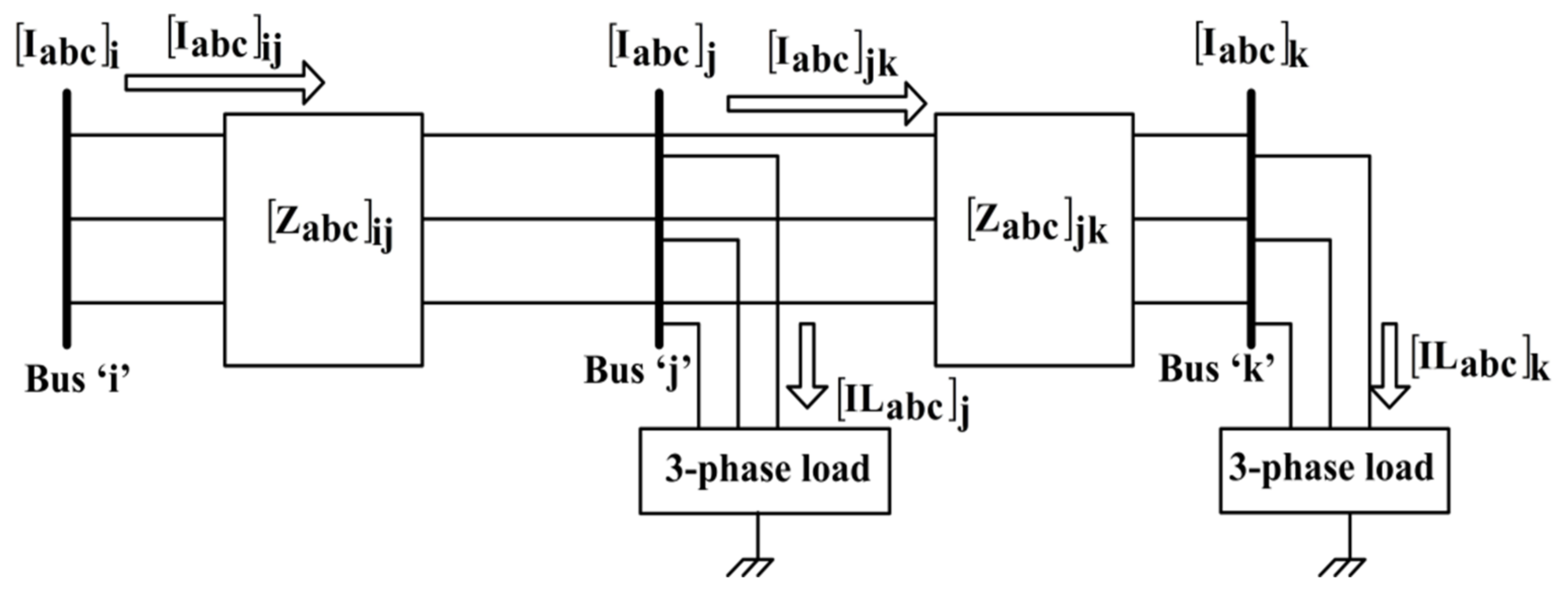
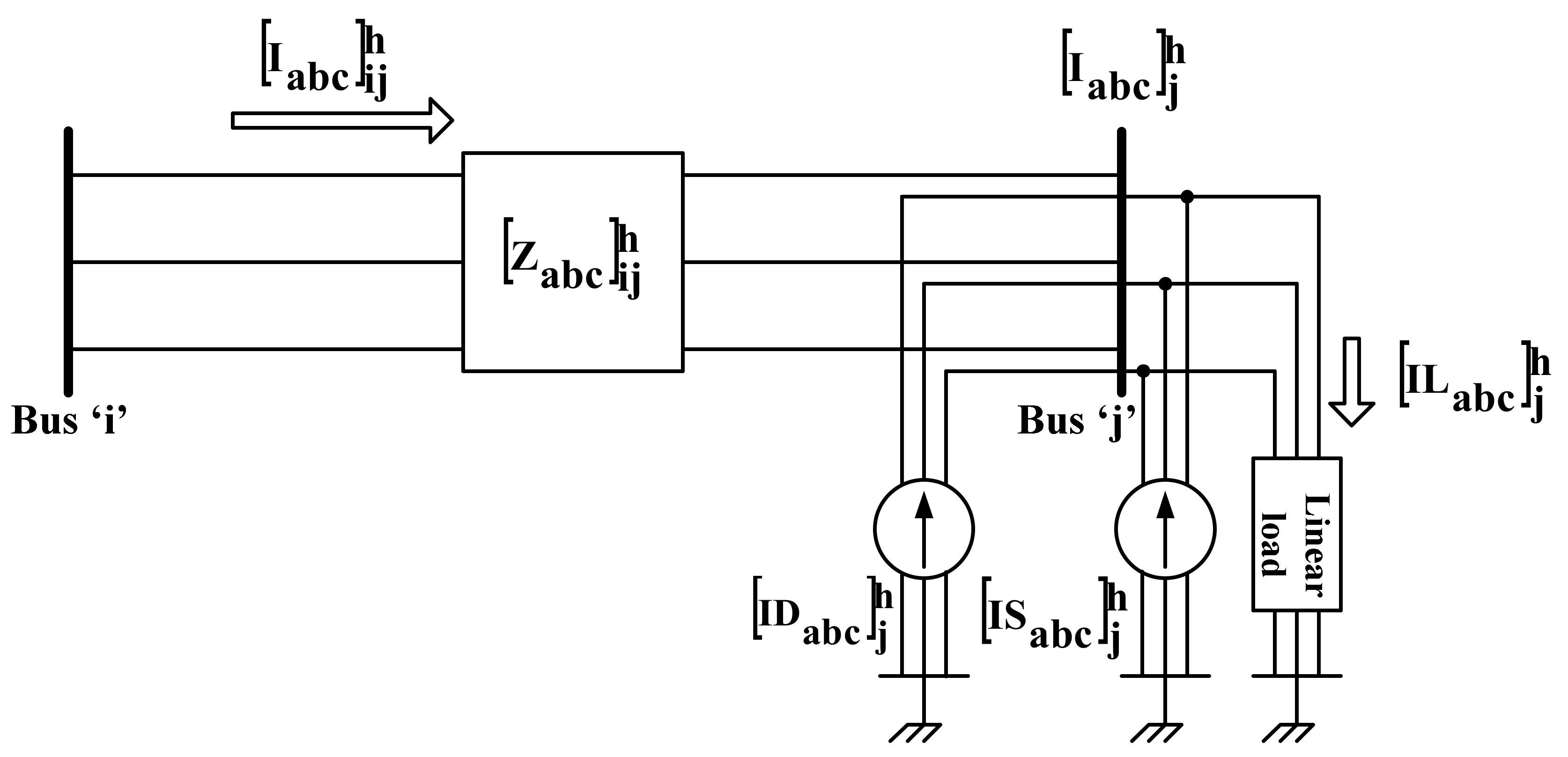
Find the net harmonic current matrix at all the buses with the harmonic current matrix drawn by the linear loads and the harmonic current injection matrix of non-linear loads and the D-STATCOM device. The current matrix drawn by the linear loads at all the buses is zero for the first iteration as the harmonic voltage at all the buses is zero for the first iteration. This is illustrated with the sample section as shown in Figure 6. The net harmonic current matrix at bus-j is given by Equation (27), and the harmonic current matrix in branch-ij is given by Equation (28):

$${\left[{\mathrm{I}}_{\mathrm{a}\mathrm{b}\mathrm{c}}\right]}_{\mathrm{j}}^{\mathrm{h}}=-{\left[\mathrm{I}{\mathrm{S}}_{\mathrm{a}\mathrm{b}\mathrm{c}}\right]}_{\mathrm{j}}^{\mathrm{h}}-{\left[\mathrm{I}{\mathrm{D}}_{\mathrm{a}\mathrm{b}\mathrm{c}}\right]}_{\mathrm{j}}^{\mathrm{h}}+{\left[\mathrm{I}{\mathrm{L}}_{\mathrm{a}\mathrm{b}\mathrm{c}}\right]}_{\mathrm{j}}^{\mathrm{h}}$$

(27)

$${\left[{\mathrm{I}}_{\mathrm{a}\mathrm{b}\mathrm{c}}\right]}_{\mathrm{i}\mathrm{j}}^{\mathrm{h}}={\left[{\mathrm{I}}_{\mathrm{a}\mathrm{b}\mathrm{c}}\right]}_{\mathrm{j}}^{\mathrm{h}}$$

(28)

where:

Figure 6. Sample section of two buses for HPFA.

${\left[{\mathrm{I}}_{\mathrm{a}\mathrm{b}\mathrm{c}}\right]}_{\mathrm{j}}^{\mathrm{h}}:$ Harmonic current matrix at bus-j for harmonic order-h;

${\left[{\mathrm{I}}_{\mathrm{a}\mathrm{b}\mathrm{c}}\right]}_{\mathrm{i}\mathrm{j}}^{\mathrm{h}}:$ Harmonic current matrix in branch-ij for harmonic order-h;

${\left[\mathrm{I}{\mathrm{L}}_{\mathrm{a}\mathrm{b}\mathrm{c}}\right]}_{\mathrm{j}}^{\mathrm{h}}:$ Harmonic current matrix drawn by linear load at bus-j for harmonic order-h;

${\left[\mathrm{I}{\mathrm{S}}_{\mathrm{a}\mathrm{b}\mathrm{c}}\right]}_{\mathrm{j}}^{\mathrm{h}}:$ Harmonic current injection matrix by non-linear load at bus-j for harmonic order-h;

${\left[\mathrm{I}{\mathrm{D}}_{\mathrm{a}\mathrm{b}\mathrm{c}}\right]}_{\mathrm{j}}^{\mathrm{h}}:$ Harmonic current injection matrix by D-STATCOM device at bus-j for harmonic order-h.

Likewise, the harmonic currents in all branches are to be obtained by moving up to the substation as explained in step 3 to step 4 in PartA for FPFA.

23.

Then, start finding the harmonic voltages at all buses downstream from the substation bus with Equation (29) as explained in step 5 in PartA:

$${\left[\begin{array}{c}{\mathrm{V}}_{\mathrm{a}}\\ {\mathrm{V}}_{\mathrm{b}}\\ {\mathrm{V}}_{\mathrm{c}}\end{array}\right]}_{\mathrm{j}}^{\mathrm{h}}={\left[\begin{array}{c}{\mathrm{V}}_{\mathrm{a}}\\ {\mathrm{V}}_{\mathrm{b}}\\ {\mathrm{V}}_{\mathrm{c}}\end{array}\right]}_{\mathrm{i}}^{\mathrm{h}}-{\left[\begin{array}{ccc}{\mathrm{Z}}_{\mathrm{a}\mathrm{a}}& {\mathrm{Z}}_{\mathrm{a}\mathrm{b}}& {\mathrm{Z}}_{\mathrm{a}\mathrm{c}}\\ {\mathrm{Z}}_{\mathrm{b}\mathrm{a}}& {\mathrm{Z}}_{\mathrm{b}\mathrm{b}}& {\mathrm{Z}}_{\mathrm{b}\mathrm{c}}\\ {\mathrm{Z}}_{\mathrm{c}\mathrm{a}}& {\mathrm{Z}}_{\mathrm{c}\mathrm{b}}& {\mathrm{Z}}_{\mathrm{c}\mathrm{c}}\end{array}\right]}_{\mathrm{i}\mathrm{j}}^{\mathrm{h}}\cdot {\left[\begin{array}{c}{\mathrm{I}}_{\mathrm{a}}\\ {\mathrm{I}}_{\mathrm{b}}\\ {\mathrm{I}}_{\mathrm{c}}\end{array}\right]}_{\mathrm{i}\mathrm{j}}^{\mathrm{h}}$$

(29)

24.

Repeat the steps 22 to 23 until the magnitude mismatch of harmonic voltages of h-order at all the busses is within the tolerance limit.

25.

Find the harmonic power loss in all branches using Equation (30). Then find the total harmonic power loss in the network for the selected harmonic order-h using Equation (31):

$${\left[\begin{array}{c}\mathrm{S}\mathrm{L}\mathrm{o}\mathrm{s}{\mathrm{s}}_{\mathrm{a}}\\ \mathrm{S}\mathrm{L}\mathrm{o}\mathrm{s}{\mathrm{s}}_{\mathrm{b}}\\ \mathrm{S}\mathrm{L}\mathrm{o}\mathrm{s}{\mathrm{s}}_{\mathrm{c}}\end{array}\right]}_{\mathrm{i}\mathrm{j}}^{\mathrm{h}}={\left[\begin{array}{c}{\left({\mathrm{V}}_{\mathrm{a}}\right)}_{\mathrm{i}}\cdot {\left({\mathrm{I}}_{\mathrm{a}}\right)}_{\mathrm{i}\mathrm{j}}^{\ast }\\ {\left({\mathrm{V}}_{\mathrm{b}}\right)}_{\mathrm{i}}\cdot {\left({\mathrm{I}}_{\mathrm{b}}\right)}_{\mathrm{i}\mathrm{j}}^{\ast }\\ {\left({\mathrm{V}}_{\mathrm{c}}\right)}_{\mathrm{i}}\cdot {\left({\mathrm{I}}_{\mathrm{c}}\right)}_{\mathrm{i}\mathrm{j}}^{\ast }\end{array}\right]}^{\mathrm{h}}-{\left[\begin{array}{c}{\left({\mathrm{V}}_{\mathrm{a}}\right)}_{\mathrm{j}}\cdot {\left({\mathrm{I}}_{\mathrm{a}}\right)}_{\mathrm{j}\mathrm{i}}^{\ast }\\ {\left({\mathrm{V}}_{\mathrm{b}}\right)}_{\mathrm{j}}\cdot {\left({\mathrm{I}}_{\mathrm{b}}\right)}_{\mathrm{j}\mathrm{i}}^{\ast }\\ {\left({\mathrm{V}}_{\mathrm{c}}\right)}_{\mathrm{j}}\cdot {\left({\mathrm{I}}_{\mathrm{c}}\right)}_{\mathrm{j}\mathrm{i}}^{\ast }\end{array}\right]}^{\mathrm{h}}$$

(30)

$${\left[\mathrm{T}\mathrm{S}\_\mathrm{l}\mathrm{o}\mathrm{s}{\mathrm{s}}_{\mathrm{a}\mathrm{b}\mathrm{c}}\right]}^{\mathrm{h}}={\displaystyle \sum _{\mathrm{b}\mathrm{r}=1}^{\mathrm{N}\mathrm{b}\mathrm{r}}\left[{\left[\mathrm{S}\mathrm{L}\mathrm{o}\mathrm{s}{\mathrm{s}}_{\mathrm{a}\mathrm{b}\mathrm{c}}\right]}_{\mathrm{b}\mathrm{r}}^{\mathrm{h}}\right]}$$

(31)

26.

Likewise, repeat the steps from 10 to 16 for all the harmonics of selected harmonic orders (h = 3, 5, 7, 9, 11, 13, and 15).

27.

Find the total harmonic loss of the network using Equation (32):

$$\left[\mathrm{T}\mathrm{o}\mathrm{t}\mathrm{a}\mathrm{l}\_\mathrm{l}\mathrm{o}\mathrm{s}\mathrm{s}\right]={\displaystyle \sum _{\mathrm{h}={\mathrm{h}}_{\mathrm{o}}}^{{\mathrm{h}}_{\mathrm{m}}}{\displaystyle \sum _{\mathrm{b}\mathrm{r}=1}^{\mathrm{N}\mathrm{b}\mathrm{r}}\left[{\left[\mathrm{S}\mathrm{L}\mathrm{o}\mathrm{s}{\mathrm{s}}_{\mathrm{a}\mathrm{b}\mathrm{c}}\right]}_{\mathrm{b}\mathrm{r}}^{\mathrm{h}}\right]}}$$

(32)

28.

The total r.m.s voltage at bus-i, say, phase ‘a’, is calculated as:

$${\left({\mathrm{V}}_{\mathrm{a}}\right)}_{\mathrm{i}}=\sqrt{{\left|{\left({\mathrm{V}}_{\mathrm{a}}\right)}_{\mathrm{i}}^1\right|}^2+{\displaystyle \sum _{\mathrm{h}={\mathrm{h}}_{\mathrm{o}}}^{{\mathrm{h}}_{\mathrm{m}}}{\left|{\left({\mathrm{V}}_{\mathrm{a}}\right)}_{\mathrm{i}}^{\mathrm{h}}\right|}^2}}$$

(33)

29.

The total harmonic distortion at every bus is calculated using Equation (34):

$${\left(\mathrm{T}\mathrm{H}\mathrm{D}\right)}_{\mathrm{i}}^{\mathrm{a}}=\frac{\sqrt{{\displaystyle \sum _{\mathrm{h}={\mathrm{h}}_{\mathrm{o}}}^{{\mathrm{h}}_{\mathrm{m}}}{\left|{\left({\mathrm{V}}_{\mathrm{a}}\right)}_{\mathrm{i}}^{\mathrm{h}}\right|}^2}}}{\left|{\left({\mathrm{V}}_{\mathrm{a}}\right)}_{\mathrm{i}}^1\right|}$$

(34)

where:

${\mathrm{h}}_{\mathrm{o}}:$ Minimum harmonic order;

${\mathrm{h}}_{\mathrm{m}}:$ Maximum harmonic order;

$\mathrm{b}\mathrm{r}:$ Branch number;

$\mathrm{N}\mathrm{b}\mathrm{r}:$ Total number of branches.

5. Results and Discussions

5.1. IEEE−13 Bus URDN

5.1.1. Fundamental Power Flow Solution for Accuracy Test

The proposed three-phase FPFA is examined on IEEE−13 bus unbalanced test feeder without interfacing of D-STATCOM device. Figure 7 shows the IEEE−13 bus feeder and its data is collected from [31]. 5000 kVA and 4.16 kV are the chosen base values for this network. The FPFA is taken 5 iterations for its convergence with tolerance for convergence is 10⁻⁴. The comparison of obtained power flow solution with IEEE solution and errors in voltage magnitudes and phase angles at every bus are presented in Table 4. Table 5 presents the comparison of obtained power loss with the IEEE losses. Insignificant values of maximum errors of 0.0005 p.u and 0.010^o for voltage magnitudes and phase angles are observed in Table 6. So that, in terms of accuracy the test results are consistent with IEEE results.

Figure 7. IEEE 13 Bus URDN.

Table 4. Fundamental voltage solution for IEEE−13 bus URDN.

Bus	Phase	Obtained Solution	IEEE Solution [31]	Error in Voltage Mag.	Error in Voltage Ang.
650	a	1 $\angle$ 0o	1 $\angle$ 0o	0.0000	0.00
	b	1 $\angle$ −120o	1 $\angle$ −120o	0.0000	0.00
	c	1 $\angle$ 120o	1 $\angle$ 120o	0.0000	0.00
RG	a	1.0625 $\angle$ 0o	1.0625 $\angle$ 0o	0.0000	0.00
	b	1.0500 $\angle$ −120o	1.0500 $\angle$ −120o	0.0000	0.00
	c	1.0687 $\angle$ 120o	1.0687 $\angle$ 120o	0.0000	0.00
632	a	1.0210 $\angle$ −2.49o	1.0210 $\angle$ −2.49o	0.0000	0.00
	b	1.0420 $\angle$ −121.72o	1.0420 $\angle$ −121.72o	0.0000	0.00
	c	1.0175 $\angle$ 117.83o	1.0170 $\angle$ 117.83o	−0.0005	0.00
671	a	0.9900 $\angle$ −5.30o	0.9900 $\angle$ −5.30o	0.0000	0.00
	b	1.0529 $\angle$ −122.34o	1.0529 $\angle$ −122.34o	0.0000	0.00
	c	0.977 $\angle$ 116.03o	0.9778 $\angle$ 116.02o	0.0001	−0.01
680	a	0.9900 $\angle$ −5.30o	0.9900 $\angle$ −5.30o	0.0000	0.00
	b	1.0529 $\angle$−122.34o	1.0529 $\angle$ −122.34o	0.0000	0.00
	c	0.9778 $\angle$ 116.03o	0.977 $\angle$ 116.02o	0.0001	−0.01
633	a	1.0180 $\angle$ −2.55o	1.0180 $\angle$ −2.56o	0.0000	0.01
	b	1.0401 $\angle$ −121.77o	1.0401 $\angle$ −121.77o	0.0000	0.00
	c	1.0148 $\angle$ 117.82o	1.0148 $\angle$ 117.82o	0.0000	0.00
634	a	0.9940 $\angle$ −3.23o	0.9940 $\angle$ −3.23o	0.0000	0.00
	b	1.0218 $\angle$ −122.22o	1.0218 $\angle$ −122.22o	0.0000	0.00
	c	0.9960 $\angle$ 117.35o	0.9960 $\angle$ 117.34o	0.0000	−0.01
645	b	1.0328 $\angle$ −121.90o	1.0329 $\angle$ −121.90o	0.0001	0.00
	c	1.0155 $\angle$ 117.86o	1.0155 $\angle$ 117.86o	0.0001	0.00
646	b	1.0311 $\angle$ −121.98o	1.0311 $\angle$ −121.98o	0.0000	0.00
	c	1.0134 $\angle$ 117.90o	1.0134 $\angle$ 117.90o	0.0000	0.01
692	a	0.9900 $\angle$ −5.30o	0.9900 $\angle$ −5.31o	0.0000	0.01
	b	1.0529 $\angle$ −122.34o	1.0529 $\angle$ −122.34o	0.0000	0.00
	c	0.9778 $\angle$ 116.03o	0.9777 $\angle$ 116.02o	−0.0001	−0.01
675	a	0.9835 $\angle$ −5.55o	0.9835 $\angle$ −5.56o	0.0000	0.01
	b	1.0553 $\angle$ −122.52o	1.0553 $\angle$ −122.52o	0.0000	0.00
	c	0.9759 $\angle$ 116.04o	0.9758 $\angle$ 116.03o	−0.0001	−0.01
684	a	0.9881 $\angle$ −5.32o	0.9881 $\angle$ −5.32o	0.0000	0.00
	c	0.9758 $\angle$ 115.92o	0.9758 $\angle$ 115.92o	0.0000	0.00
611	c	0.9738 $\angle$ 115.78o	0.9738 $\angle$ 115.78o	0.0000	0.00
652	a	0.9825 $\angle$ −5.24o	0.9825 $\angle$ −5.25o	0.0000	0.01

Table 5. Power loss in IEEE−13 bus URDN.

Phase	Obtained Power Loss		IEEE Loss [31]
	Active (kW)	Reactive (kVAR)	Active (kW)	Reactive (kVAR)
a	39.13	152.62	39.11	152.59
b	−4.74	42.27	−4.70	42.22
c	76.59	129.69	76.65	129.85
Total	110.98	324.57	111.13	324.66

Table 6. Power loss in IEEE−13 bus URDN.

Harmonic Order	Harmonic Power Loss
	APL (kW)	RPL (kVAR)
3	0.7958	6.5165
5	0.0856	1.1483
7	0.0072	0.1183
9	0.0043	0.0902
11	0.0008	0.0164
13	0.0008	0.0226
15	0.0010	0.0340
Total harmonic loss	0.8983	7.9464
Fundamental loss	147.33	433.54
Total power loss	148.23	441.49

5.1.2. Fundamental and Harmonic Power Flow Solutions without D-STATCOM

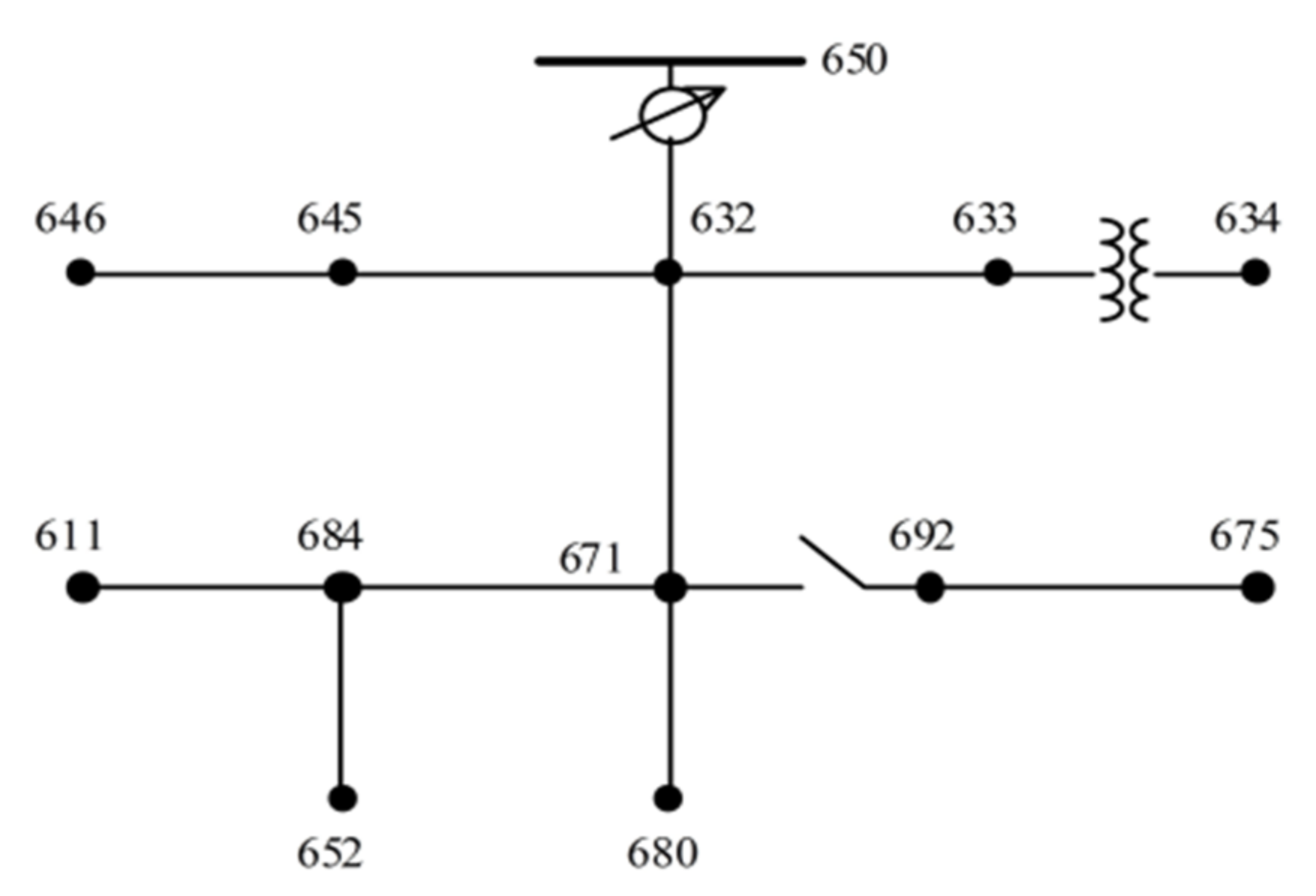
The regulator between buses 650 and 632 is removed and the capacitor banks at bus 675 and 611 are removed from the network. The data for the harmonic load composition and current spectra of harmonic loads aretaken from [32]. The convergence tolerance is taken as 10⁻⁴. Table 6 presents the harmonic power losses and total power loss of the network including fundamental and harmonic loss. The harmonic voltage solutions for the selected range of harmonics of order 3, 5, 7, 9, 11, 13, and 15 are presented in Table 7. Table 8 presents the fundamental r.m.s profile, the total harmonic voltage profile, and the THD %. It is observed from Table 8 that the maximum THD % on the network is 5.2263 at bus−611 for c-phase, and in [2], it was reported that the maximum THD % at bus−611 is 5.23. Therefore, the results of the proposed HPFA are almost matches the literature in terms of accuracy. To see the impact of the D-STATCOM on the fundamental r.m.s voltage profile, the total r.m.s voltage profile, the fundamental and harmonic power loss, and the THD %, the results of this case study are taken as benchmarks.

Table 7. Fundamental r.m.s voltage, total r.m.s voltages, and THD % in IEEE−13 bus URDN.

Bus	Phase	S. No	Fundamental r.m.s Voltage	Total r.m.s Voltage	THD %
650	a	1	1 $\angle$ 0o	1	0
	b	2	1 $\angle$ −120o	1	0
	c	3	1 $\angle$ 120o	1	0
632	a	4	0.9498 $\angle$ −2.7462o	0.9500	1.9173
	b	5	0.9839 $\angle$ −121.6817o	0.9839	0.4974
	c	6	0.9300 $\angle$ 117.8000o	0.9302	2.2737
671	a	7	0.9109 $\angle$ −5.8987o	0.9117	4.0623
	b	8	0.9875 $\angle$ −122.2091o	0.9875	1.0363
	c	9	0.8717 $\angle$ 115.9500o	0.8728	4.9409
680	a	10	0.9109 $\angle$ −5.8987o	0.9117	4.0623
	b	11	0.9875 $\angle$ −122.2091o	0.9875	1.0363
	c	12	0.8717 $\angle$ 115.9500o	0.8728	4.9409
633	a	13	0.9466 $\angle$ −2.8223o	0.9468	1.9098
	b	14	0.9819 $\angle$ −121.7315o	0.9819	0.4919
	c	15	0.9271 $\angle$ 117.7946o	0.9273	2.2648
634	a	16	0.9207 $\angle$ −3.6073o	0.9209	1.8801
	b	17	0.9624 $\angle$ −122.2445o	0.9624	0.4873
	c	18	0.9064 $\angle$ 117.2178o	0.9066	2.2406
645	b	19	0.9745 $\angle$ −121.8646o	0.9745	0.4991
	c	20	0.9283 $\angle$ 117.8225o	0.9286	2.2769
646	b	21	0.9729 $\angle$ −121.9382o	0.9729	0.5000
	c	22	0.9264 $\angle$ 117.8696o	0.9267	2.2815
692	a	23	0.9109 $\angle$ −5.8987o	0.9117	4.0623
	b	24	0.9875 $\angle$ −122.2091o	0.9875	1.0363
	c	25	0.8717 $\angle$ 115.9500o	0.8728	4.9409
675	a	26	0.9025 $\angle$ −6.0795o	0.9034	4.3128
	b	27	0.9887 $\angle$ −122.3037o	0.9887	1.0491
	c	28	0.8678 $\angle$ 116.0660o	0.8689	5.0687
684	a	29	0.9093 $\angle$ −5.9502o	0.9100	4.0765
	c	30	0.8684 $\angle$ 115.9163o	0.8695	5.0741
611	c	31	0.8651 $\angle$ 115.8365o	0.8663	5.2263
652	a	32	0.9041 $\angle$ −5.8755o	0.9049	4.0900

Table 8. Fundamental and Harmonic power loss for IEEE−13 URDN with D-STATCOM.

Harmonic Order	Harmonic Power Loss
	Active (kW)	Reactive (kVAR)
3	0.7836	6.3935
5	0.0841	1.1282
7	0.0071	0.1168
9	0.0043	0.0886
11	0.0008	0.0160
13	0.0008	0.0223
15	0.0009	0.0336
Total harmonic loss	0.8816	7.7991
Fundamental Loss	135.34	396.63
Total power loss	136.22	404.43

5.1.3. IEEE−13 Bus URDN with D-STATCOM

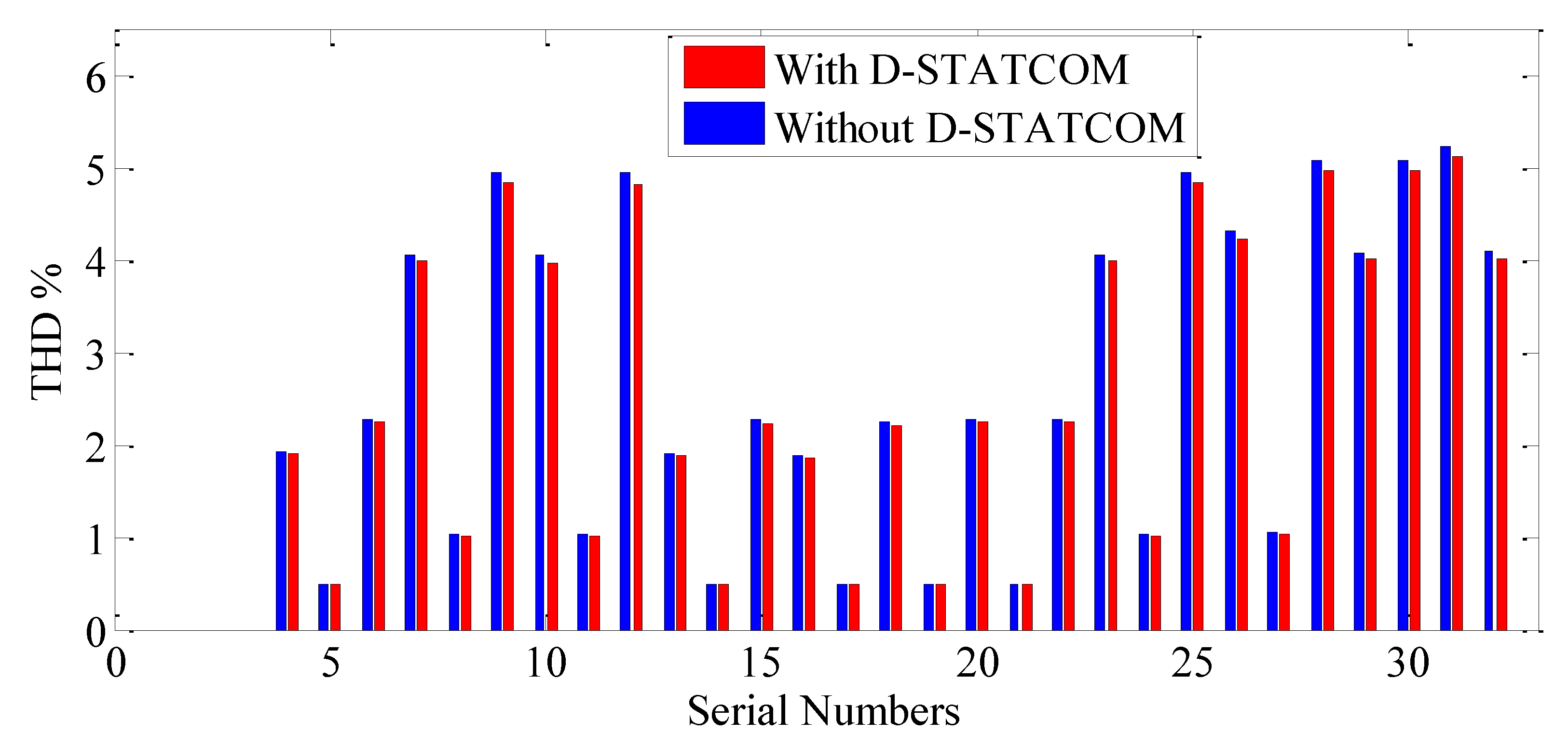
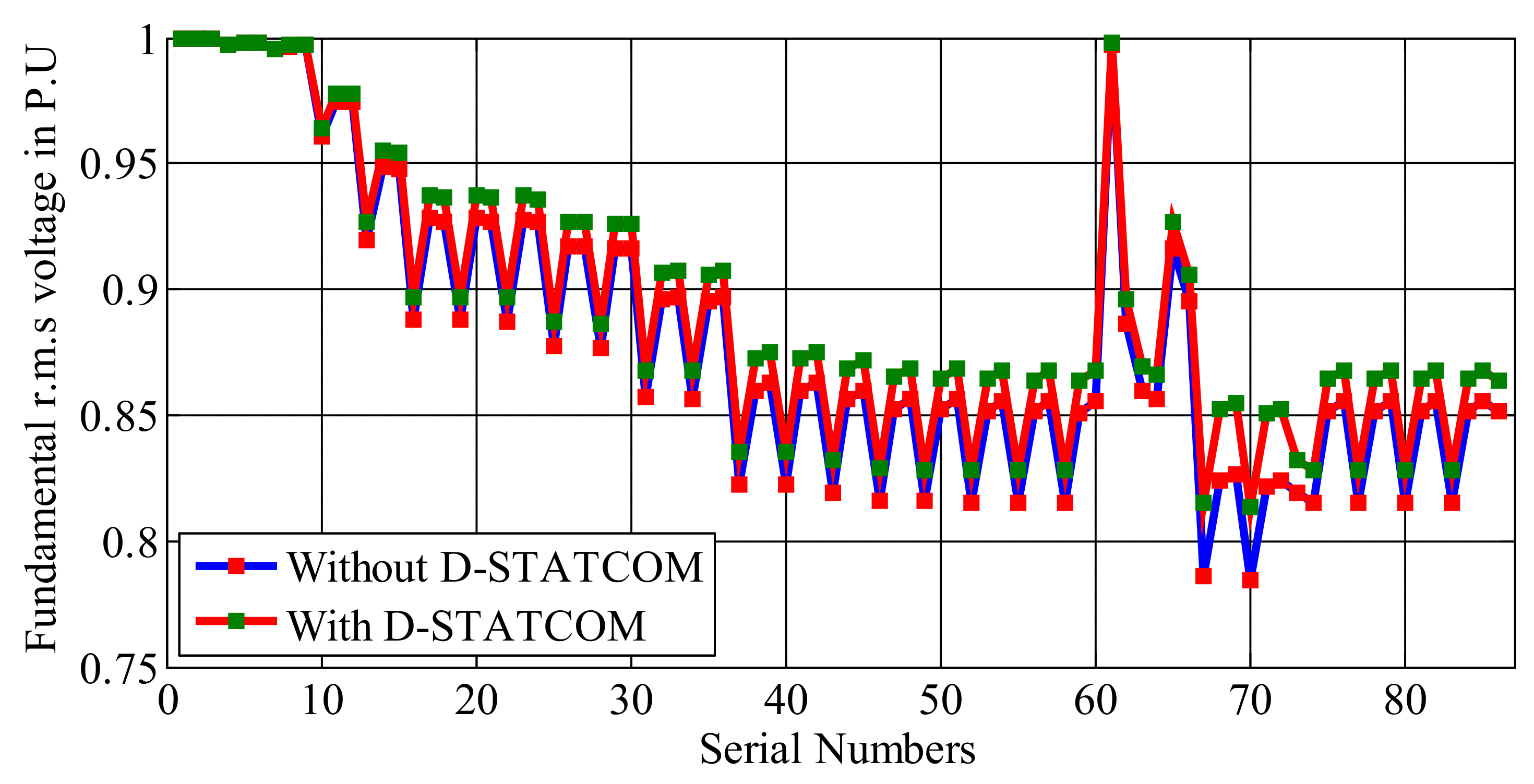
In this case, a three-phase D-STATCOM is integrated at bus 680. The D-STATCOM is modelled as a PV model with its real power generation set to zero and the lower limit and upper limit for the three-phase reactive power generation are 100 kVAR and 1000 kVAR, respectively. The phase voltages specified at this bus are 1 p.u. Table 8 presents the harmonic power loss and total power loss (including fundamental and harmonic power loss). In comparison with Table 6, it is observed that the integration of the D-STATCOM into the network reduces both the fundamental and harmonic power losses, thereby the total power loss in the network is also reduced. Table 9 presents the fundamental r.m.s voltage profile, the total r.m.s voltage profile, and the THD %.In comparison with Table 7, it is observed that there is an improvement in fundamental r.m.s voltage profile. The minimum fundamental r.m.s voltage in the network without D-STATCOM is 0.8651 p.uat bus−611 for c-phase, whereas its value is 0.8763 p.u at bus−611 for c-phase with integration of D-STATCOM. The maximum THD % in the network is reduced from 5.2263 to 5.1133 with integration of D-STATCOM. Figure 8 shows the comparison of THD % with and without integration of D-STATCOM. Figure 9 presents the comparison of fundamental r.m.s voltages on the network for the two case studies.

Table 9. Fundamental r.m.s voltages, total r.m.s voltages, and THD % in IEEE−13 bus URDN with D-STATCOM.

Bus	Phase	Fundamental r.m.s Voltage	Total r.m.s Voltage in p.u	THD %
650	a	1.0000$\angle$0o	1	0
	b	1.0000$\angle$−120o	1	0
	c	1.0000$\angle$120o	1	0
632	a	0.9545$\angle$−2.8433o	0.9547	1.8920
	b	0.9883$\angle$−121.7039o	0.9883	0.4923
	c	0.9355$\angle$117.6975o	0.9357	2.2404
671	a	0.9204$\angle$−6.0689o	0.9211	3.9865
	b	0.9961$\angle$−122.2496o	0.9962	1.0211
	c	0.8829$\angle$115.7512o	0.8839	4.8346
680	a	0.9227$\angle$−6.1274o	0.9234	3.9764
	b	0.9983$\angle$−122.2605o	0.9983	1.0189
	c	0.8855$\angle$115.6856o	0.8865	4.8205
633	a	0.9512$\angle$−2.9186o	0.9514	1.8846
	b	0.9863$\angle$−121.7535o	0.9863	0.4869
	c	0.9326$\angle$117.6923o	0.9329	2.2317
634	a	0.9255$\angle$−3.6957o	0.9256	1.8556
	b	0.9669$\angle$−122.2618o	0.9669	0.4823
	c	0.9121$\angle$117.1225o	0.9123	2.2082
645	b	0.9789$\angle$−121.8864o	0.9789	0.4940
	c	0.9338$\angle$117.7205o	0.9341	2.2436
646	b	0.9773$\angle$−121.9600o	0.9773	0.4948
	c	0.9319$\angle$117.7674o	0.9322	2.2482
692	a	0.9204$\angle$−6.0689o	0.9211	3.9865
	b	0.9961$\angle$−122.2496o	0.9962	1.0211
	c	0.8829$\angle$115.7512o	0.8839	4.8346
675	a	0.9121$\angle$−6.2456o	0.9129	4.2312
	b	0.9973$\angle$−122.3429o	0.9973	1.0335
	c	0.8790$\angle$115.8645o	0.8801	4.9586
684	a	0.9187$\angle$−6.1203o	0.9194	4.0007
	c	0.8796$\angle$115.7184o	0.8807	4.9647
611	c	0.8763$\angle$115.6396o	0.8775	5.1133
652	a	0.9135$\angle$−6.0456o	0.9142	4.0140

Figure 8. Comparison of THD % for case studies on IEEE−13 URDN.

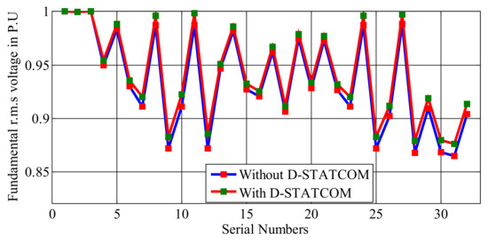
Figure 9. Comparison of fundamental r.m.svoltages for case studies on IEEE−13 URDN.

5.2. IEEE−34 Bus URDN

The date for the IEEE−34 bus URDN is taken from [31]. The base values selected for the system are 2500 kVA and 24.9 kV. The load composition at spot loads for harmonic analysis is presented in Table 10. The data for the current spectra of harmonic loads aretaken from [32]. The convergence tolerance for both fundamental and harmonic power flows is 10⁻⁴. The case studies on the network are presented in Table 11. The rating and location of the D-STATCOM device for Case2 is presented in Table 11. Table 12 presents the fundamental r.m.s voltage profile, the total r.m.s voltage profile, and the THD % for Case1. The test results of Case1 are used as a benchmark to see the fundamental and harmonic impacts of D-STATCOM on the network. The summary of results for the case studies is presented in Table 13. In Case2, which has integrations of two D-STATCOM devices, the maximum THD% is observed to be 5.2567 which is less than in Case 1. The number of phases effected with a THD% more than fiveis reduced from fourto twofrom Case 1 to Case 2. From Case 1 to Case 2, it is found that the minimum fundamental voltage on the network is improved from 0.7641 p.u to 0.8137 p.u at bus 890 for the a-phase.The fundamental power loss and the total power loss including harmonic loss of the network reduced in Case 2 in comparison with Case 1. Figure 10 shows the comparison of THD % with and without the integration of the D-STATCOM. Figure 11 shows the comparison of the fundamental r.m.s voltages on the network for the two case studies.

Table 10. Load composition of spot loads in IEEE−34 bus URDN.

Bus No.	Load Composition
	Non-Linear Loads			Linear Loads
	Fluorescent Light Banks	Adjustable Speed Drives	Composite Residential Loads
830	None	None	80%	20%
844	30%	30%	30%	10%
848	30%	30%	30%	10%
890	30%	None	60%	10%
860	30%	30%	30%	10%
840	30%	30%	30%	10%

Table 11. Case studies on IEEE−34 bus URDN.

Case Study	Description
Case 1 (Without D-STATCOM)	Voltage regulator is taken off between bus−614 and bus−650 and bus−852 and bus−832. Capacitor banks are taken off at bus−844 and bus−848. Load composition of spot loads as in Table 9
Case 2 (With D-STATCOM)	Three-phase D-STATCOM placed at bus 890 is modeled as PV bus with P = 0 and three-phase reactive power limits: 100 ≤ Q ≤ 500 kVAR. Three-phase D-STATCOM placed at bus 650 is modeled as PV bus with P = 0 and three-phase reactive power limits: 100 ≤ Q ≤ 500 kVAR.

Table 12. Fundamental r.m.s voltages, total r.m.s voltages, and THD % in the IEEE−34 bus URDN for Case 1.

Bus No.	S. No.	Ph.	Total r.m.s Voltages in p.u	THD %	Bus No	S. No.	Ph.	Total r.m.sVoltages in p.u	THD %
800	1	a	1	0		46	a	0.8169	4.8628
	2	b	1	0	834	47	b	0.8531	4.0835
	3	c	1	0		48	c	0.8570	4.5399
802	4	a	0.9972	0.0541		49	a	0.8168	4.8691
	5	b	0.9980	0.0481	842	50	b	0.8530	4.0888
	6	c	0.9981	0.0531		51	c	0.8569	4.5458
806	7	a	0.9953	0.0908		52	a	0.8164	4.8990
	8	b	0.9967	0.0808	844	53	b	0.8524	4.1147
	9	c	0.9969	0.0891		54	c	0.8565	4.5742
808	10	a	0.9605	0.7955		55	a	0.8162	4.9094
	11	b	0.9745	0.6983	846	56	b	0.8519	4.1261
	12	c	0.9742	0.7706		57	c	0.8562	4.5841
812	13	a	0.9200	1.6825		58	a	0.8162	4.9109
	14	b	0.9488	1.4531	848	59	b	0.8518	4.1276
	15	c	0.9479	1.6045		60	c	0.8562	4.5855
814	16	a	0.8880	2.4435	810	61	b	0.9975	0.0562
	17	b	0.9284	2.0813	818	62	a	0.8869	2.4466
	18	c	0.9271	2.2994	820	63	a	0.8599	2.5235
850	19	a	0.8880	2.4438	822	64	a	0.8564	2.5339
	20	b	0.9284	2.0815	826	65	b	0.9169	2.3333
	21	c	0.9271	2.2997	856	66	b	0.8954	2.8693
816	22	a	0.8877	2.4526		67	a	0.7875	5.5150
	23	b	0.9281	2.0888	888	68	b	0.8248	4.8565
	24	c	0.9268	2.3079		69	c	0.8275	5.1312
824	25	a	0.8778	2.7468		70	a	0.7853	5.5791
	26	b	0.9171	2.3328	890	71	b	0.8228	4.9085
	27	c	0.9173	2.5798		72	c	0.8252	5.1873
828	28	a	0.8769	2.7713	864	73	a	0.8203	4.7018
	29	b	0.9162	2.3529	860	74	a	0.8164	4.8734
	30	c	0.9165	2.6025		75	b	0.8526	4.0921
830	31	a	0.8574	3.3823		76	c	0.8566	4.5493
	32	b	0.8961	2.8557		77	a	0.8162	4.8779
	33	c	0.8974	3.1673	836	78	b	0.8522	4.0967
854	34	a	0.8569	3.3981		79	c	0.8565	4.5531
	35	b	0.8956	2.8688		80	a	0.8162	4.8790
	36	c	0.8969	3.1820	840	81	b	0.8522	4.0976
852	37	a	0.8233	4.5667		82	c	0.8564	4.5542
	38	b	0.8603	3.8340		83	a	0.8162	4.8779
	39	c	0.8634	4.2626	862	84	b	0.8522	4.0968
832	40	a	0.8233	4.5671		85	c	0.8565	4.5530
	41	b	0.8603	3.8342	838	86	b	0.8520	4.0977
	42	c	0.8634	4.2629	---
858	43	a	0.8203	4.7018
	44	b	0.8570	3.9475
	45	c	0.8604	4.3890

Table 13. Summary of results for the case studies on IEEE−34 bus URDN.

Case Study	Min. Fundamental Voltage, p.u	Min. Total r.m.sVoltage, p.u	Max. THD%	No. of Phases of Buses (THD > 5%)
Case 1	0.7841 at bus−890, a-phase	0.7853 at bus−890, a-phase	5.5791 at bus−890, a-phase	4
Case 2	0.8137 at bus−890, a-phase	0.8148 at bus−890, a-phase	5.2567 at bus−890, a-phase	2
Case study	Total fundamental power loss		Total power loss including total harmonic loss
	Active (kW)	Reactive (kVAR)	Active (kW)	Reactive (kVAR)
Case 1	260.89	180.49	264.56	188.15
Case 2	227.69	155.82	231.23	163.21

Figure 10. Comparison of THD% for case studies on IEEE−34 URDN.

Figure 11. Comparison of fundamental r.m.svoltages for case studies on IEEE−34 URDN.

6. Conclusions

This paper proposes new three-phase PFAs for URDN with the presence of linear and non-linear loads and D-STATCOM devices. These PFAs can give both fundamental and harmonic power flow solutions with/without the presence of D-STATCOM devices. The developed BNM and BRNM make both the FPFA and HPFA simple. These matrices are developed by exploiting the radial topology in distribution networks. This method uses the basic concepts of circuit theory, and they can be easily understood. In this paper, the linear loads are modeled as a series combination of resistance and reactance, and non-linear loads are modeled as constant current sources with its magnitude and angle obtained from the current spectra. The harmonic current injections from the D-STATCOM are assumed as zero. The proposed FPFA and HPFA are tested on the IEEE−13 bus URDN, and the results are found to be accurate with the literature. The test studies are carried on the IEEE−13 bus and IEEE−34 bus URDN, and the results of the case studies show thatthere is an improvement in the fundamental voltage profile, a reduction in the fundamental and harmonic power loss, and a reduction in THD% with the integration of D-STATCOM devices.

References

- Burch, R.; Chang, G.K.; Grady, M.; Hatziadoniu, C.; Liu, Y.; Marz, M.; Ortmeyer, T.; Xu, W.; Ranade, S.; Ribeiro, P. Impact of aggregate linear load modeling on harmonic analysis: A comparison of common practice and analytical models. IEEETrans. Power Deliv. 2003, 18, 625–630. [Google Scholar] [CrossRef]
- Yang, N.-C.; Le, M.-D. Three-phase harmonic power flow by direct ZBUS method for unbalanced radial distribution systems with passive power filters. IET Gener. Transm. Distrib. 2016, 10, 3211–3219. [Google Scholar] [CrossRef]
- Milovanović, M.; Radosavljević, J.; Perović, B.; Dragičević, M. Power flow in radial distribution systems in the presence of harmonics. Int. J. Electr. Eng. Comput. 2018, 2, 11–19. [Google Scholar] [CrossRef]
- Amini, M.A.; Jalilian, A.; Behbahani, M.R.P. Fast network reconfiguration in harmonic polluted distribution network based on developed backward/forward sweep harmonic load flow. Electr. Power Syst. Res. 2019, 168, 295–304. [Google Scholar] [CrossRef]
- Milovanović, M.; Radosavljević, J.; Perović, B. A backward/forward sweep power flow method for harmonic polluted radial distribution systems with distributed generation units. Int. Trans. Electr. Energy Syst. 2019, 30, e12310. [Google Scholar] [CrossRef]
- Nduka, O.S.; Ahmadi, A.R. Data-driven robust extended computer-aided harmonic power flow analysis. IET Gener. Transm. Distrib. 2020, 14, 4398–4409. [Google Scholar] [CrossRef]
- Hernandez, J.C.; Ruiz-Rodriguez, F.J.; Jurado, F.; Sanchez-Sutil, F. Tracing harmonic distribution and voltage unbalance in secondary radial distribution networks with photovoltaic uncertainties by a multiphase harmonic load flow. Electr. Power Syst. Res. 2020, 185, 1–18. [Google Scholar] [CrossRef]
- Ruiz-Rodriguez, F.J.; Hernandez, J.C.; Jurado, F. Iterative harmonic load flow by using the point-estimate method and complex affine arithmetic for radial distribution systems with photovoltaic uncertainties. Electr. Power Energy Syst. 2020, 118, 1–16. [Google Scholar] [CrossRef]
- El-Fergany, A.; Abdelaziz, A.Y. Cuckoo Search-based Algorithm for Optimal Shunt Capacitors Allocations in Distribution Networks. Electr. Power Compon. Syst. 2013, 41, 1567–1581. [Google Scholar] [CrossRef]
- Abdelaziz, A.Y.; Ali, E.S.; Abd Elazim, S.M. Flower Pollination Algorithm for Optimal Capacitor Placement and Sizing in Distribution Systems. Electr. Power Compon. Syst. J. 2016, 44, 544–555. [Google Scholar] [CrossRef]
- Satish, R.; Kantarao, P.; Vaisakh, K. A new algorithm for impacts of multiple DGs and D-STATCOM in unbalanced radial distribution networks. Int. J. Renew. Energy Technol. 2021, 12, 221–242. [Google Scholar] [CrossRef]
- Satish, R.; Vaisakh, K.; Abdelaziz, A.Y.; El-Shahat, A. A Novel Three-phase Power Flow Algorithm for Evaluation of Impact of Renewable Energy Sources and D-STATCOM Device in Unbalanced Radial Distribution Networks. Energies 2021, 14, 6152. [Google Scholar] [CrossRef]
- Othman, M.M.; Hegazy, Y.G.; Abdelaziz, A.Y. Electrical Energy Management in Unbalanced Distribution Networks using Virtual Power Plant Concept. Electr. Power Syst. Res. 2017, 145, 157–165. [Google Scholar] [CrossRef]
- Abdelaziz, A.Y.; Hegazy, Y.G.; El-Khattam, W.; Othman, M.M. A Multi objective Optimization for Sizing and Placement of Voltage Controlled Distributed Generation Using Supervised Big Bang Big Crunch Method. Electr. Power Compon. Syst. 2015, 43, 105–117. [Google Scholar] [CrossRef]
- Abdelaziz, A.Y.; Hegazy, Y.G.; El-Khattam, W.; Othman, M.M. Optimal Planning of Distributed Generators in Distribution Networks Using Modified Firefly Method. Electr. Power Compon. Syst. 2015, 43, 320–333. [Google Scholar] [CrossRef]
- Rohouma, W.; Balog, R.S.; Peerzada, A.A.; Begovic, M.M. D-STATCOM for harmonic mitigation in low voltage distribution network with high penetration of nonlinear loads. Renew. Energy 2020, 145, 1449–1464. [Google Scholar] [CrossRef]
- Sirjani, R.; Jordehi, A.R. Optimal placement and sizing of distribution static compensator (D-STATCOM) in electric distribution networks: A review. Renew. Sustain. Energy Rev. 2017, 77, 688–694. [Google Scholar] [CrossRef]
- Rezaeian-Marjani, S.; Galvani, S.; Talavat, V.; Farhadi-Kangarlu, M. Optimal allocation of D-STATCOM in distribution networks including correlated renewable energy sources. Electr. Power Energy Syst. 2020, 122, 1–14. [Google Scholar] [CrossRef]
- Patel, S.K.; Arya, S.R.; Maurya, R. Optimal Step LMS-Based Control Algorithm for DSTATCOM in Distribution System. Electr. Power Compon. Syst. 2019, 47, 675–691. [Google Scholar] [CrossRef]
- Singh, B.; Singh, S. GA-based optimization for integration of DGs, STATCOM and PHEVs in distribution systems. Energy Rep. 2019, 5, 84–103. [Google Scholar] [CrossRef]
- Badoni, M.; Singh, A.; Singh, B.; Saxena, H. Real-time implementation of active shunt compensator with adaptive SRLMMN control technique for power quality improvement in the distribution system. Int. Trans. Electr. Energy Syst. 2020, 14, 1598–1606. [Google Scholar] [CrossRef]
- Selvaraj, G.; Rajangam, K. Multi-objective grey wolf optimizer algorithm for combination of network reconfiguration and D-STATCOM allocation in distribution system. Int. Trans. Electr. Energy Syst. 2019, 29, e12100. [Google Scholar] [CrossRef]
- Kersting, W.H. Distribution System Modeling and Analysis, 4th ed.; CRC Press: Boca Raton, FL, USA, 2017. [Google Scholar]
- Task Force on Harmonics Modeling and Simulation. Modeling and simulation of the propagation of harmonics in electric power networks I. Concepts, models, and simulation techniques. IEEE Trans. Power Deliv. 1996, 11, 452–465. [Google Scholar] [CrossRef]
- Chen, T.H.; Chang, J.D.; Chang, Y.L. Models of grounded mid-tap open-wye and open-delta connected transformers for rigorous analysis of a distribution system. IEEE Proc. Gener. Transm. Distrib. 1996, 143, 82–88. [Google Scholar] [CrossRef]
- Arrillaga, J.; Bradley, D.A.; Bodger, P.S. Power System Harmonics, 1st ed.; Wiley: Hoboken, NJ, USA, 1985. [Google Scholar]
- Yang, Z.; Shen, C.; Crow, M.L.; Zhang, L. An improved STATCOM model for power flow analysis. In Proceedings of the 2000 Power Engineering Society Summer Meeting, Seattle, WA, USA, 16–20 July 2000; pp. 1121–1126. [Google Scholar]
- Jazebi, S.; Hosseinian, S.H.; Vahidi, B. DSTATCOM allocation in distribution networks considering reconfiguration using differential evolution algorithm. Energy Convers. Manag. 2011, 52, 2777–2783. [Google Scholar] [CrossRef]
- Das, D.; Nagi, H.S.; Kothari, D.P. Novel method for solving radial distribution networks. IEEE Proc. Gener. Transm. Distrib. 1994, 141, 291–298. [Google Scholar] [CrossRef]
- Shirmohammadi, D.; Carol, S.; Cheng, A. A Three phase power flow method for real time distribution system analysis. IEEE Trans. Power Syst. 1995, 10, 671–679. [Google Scholar]
- Radial Distribution Test Feeders. Available online: http://sites.ieee.org/pes-testfeeders/resources (accessed on 28 September 2021).
- Abu-Hashim, R.; Burch, R.; Chang, G.; Grady, M.; Gunther, E.; Halpin, M.; Xu, W.; Marz, M.; Sim, T.; Liu, Y.; et al. Test systems for harmonic modeling and simulation. IEEE Trans. Power Deliv. 1999, 14, 579–587. [Google Scholar] [CrossRef]
Publisher’s Note: MDPI stays neutral with regard to jurisdictional claims in published maps and institutional affiliations. |
© 2021 by the authors. Licensee MDPI, Basel, Switzerland. This article is an open access article distributed under the terms and conditions of the Creative Commons Attribution (CC BY) license (https://creativecommons.org/licenses/by/4.0/).