
A Novel Three-Phase Harmonic Power Flow Algorithm for Unbalanced Radial Distribution Networks with the Presence of D-STATCOM Devices


Abstract
:1. Introduction
2. Network Components and Their Modeling
2.1. Overhead or Underground Distribution Lines
2.2. Loads
2.2.1. Linear Loads
2.2.2. Non-Linear Loads
2.3. Capacitor Banks
2.4. Tree-Phase Transformer
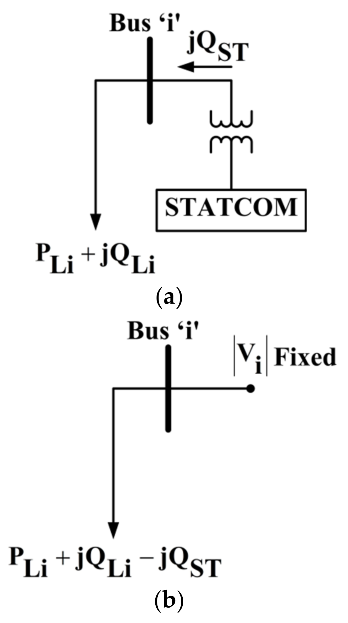
2.5. D-STATCOM
3. Algorithm for Developing BNM and BRNM
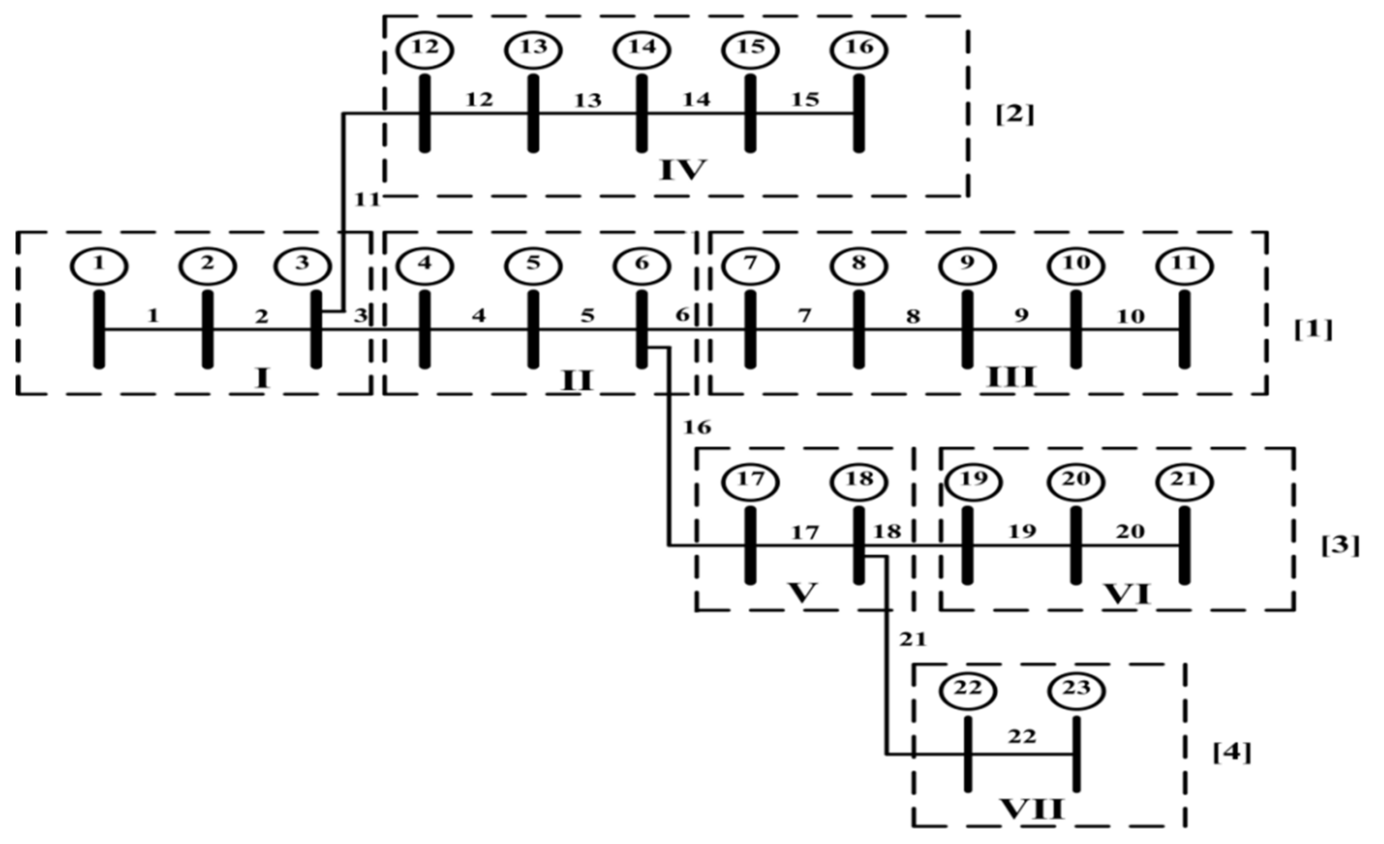
- Start with BN = 1.Read the RE of BN, i.e., 2. Then, check how many times this 2 appears in the SE row. Inthe above table, it appears one time. That means bus 2 is the sending end for only one branch. Fill these RE 2 and BN 1 in two different matrices (BNM and BRNM) as the first row and first column elements. Then, increase the column number by one.
- Increase the BN (i.e., BN = 2), and read the RE of BN, i.e., 3. Then, as in step 1, check for the appearance of 3 in SE row. The bus 3 appears two times. That means that, from the bus 3, two branches are leaving. Then, fill these RE 3 and BN 2 into the same variables as the first row and present the column elements. Name this row elements as section-I. Now increase the row number by one and set the column number to one.
- Similarly, increase the BN, and read the RE of BN. Then, check for the appearance of this RE in the SE row. If it appears one time, then fill these RE and BN values as the present row and present column elements of the variables BNM and BRNM. Then increase the column number by one and repeat step 4. If it does not appears or appears more than one time in the SE row, then fill the corresponding RE and BN values as present row and present column elements. Then identify this row as a section. Then increase the row number by one and set the column number to one and repeat the step 4.

4. Three-Phase HPFA with Non-Linear Loads and D-STATCOM Devices
- The voltages at all busses are assigned as substation bus voltage.
- Find the line current matrix serving the load at all buses.
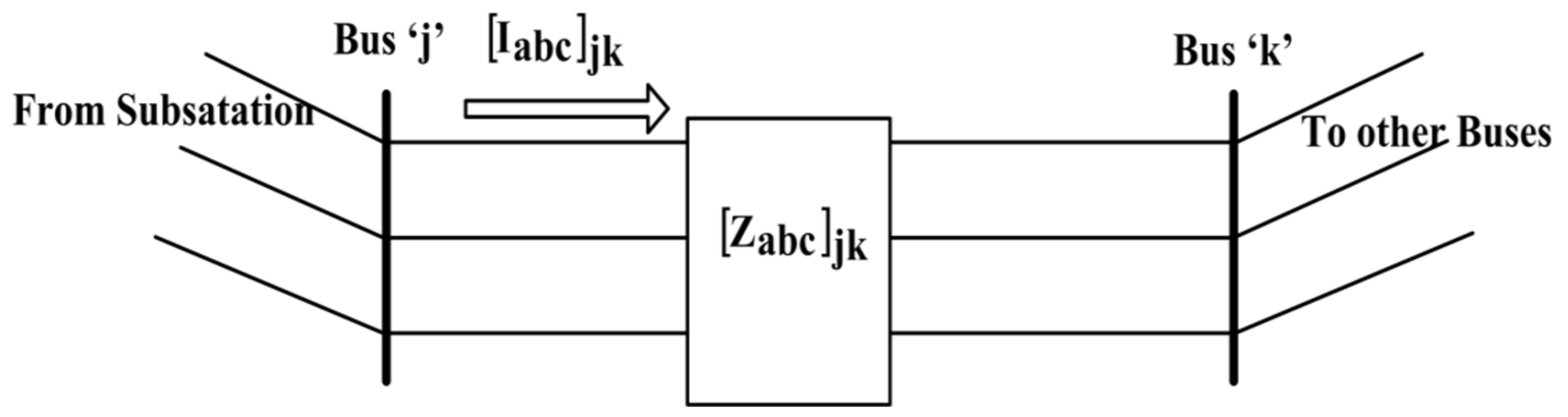
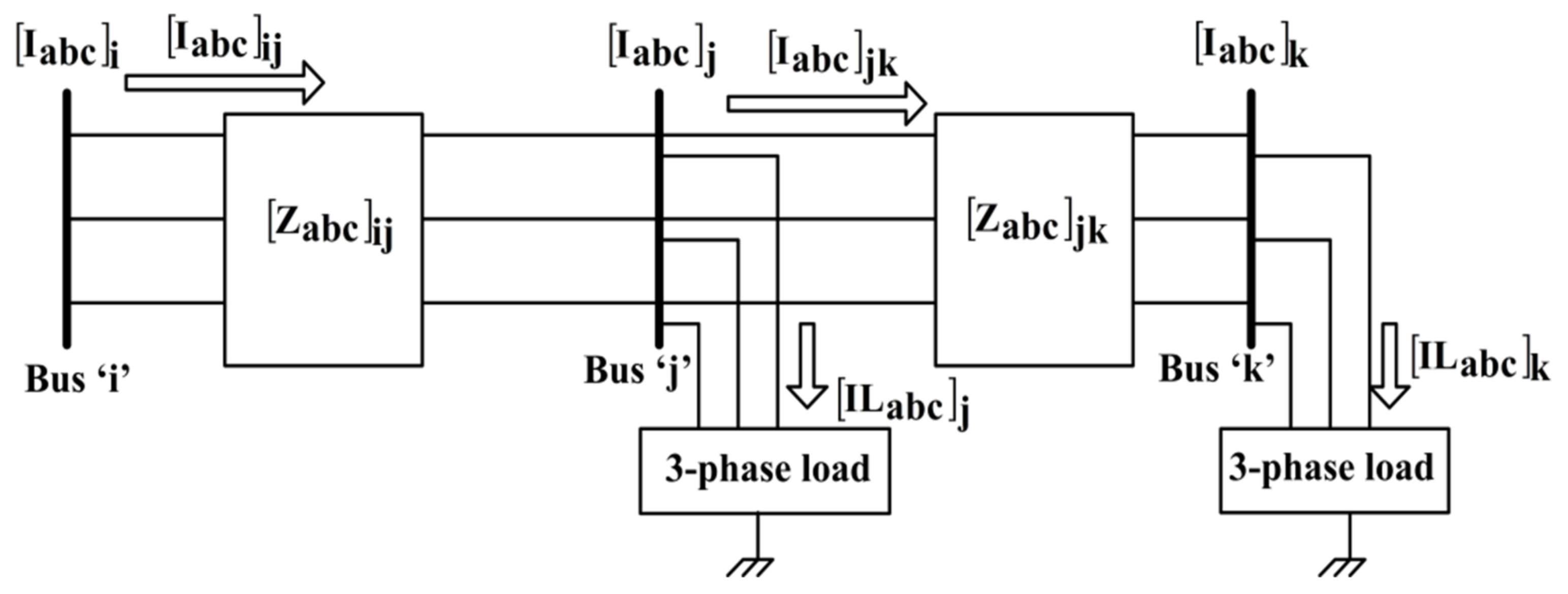
- Start with collecting line current matrix at bus−23 (the tail bus in section-VII in BNM), and thereby find the line current matrix for branch−22 (the tail branch in section-VII in BRNM). Then, continue to the bus−22 and branch−21 to find the line current matrix at the bus and line current matrix in branch, respectively. From Figure 4, the following equations are obtained by applying the KCL at every bus:where:Line current matrix at bus-k;Line current in branch-jk;Load current matrix at bus-k;Line current matrix drawn by shunt admittance at bus-k;Line current matrix drawn by capacitor bank at bus-k, if any.
- Now go to section-VI and repeat procedure as in step 5 to find the line current matrix at the head bus and line current matrix for head branch. Similarly, proceed up to section-I and find the line current matrix up to bus−1 and line current matrix up to branch−1.
- Now start with head bus in section-I and continue to the tail bus in section-I by finding the phase voltage matrix at all buses with Equation (2). Then, go to the next section and repeat the same procedure.
- Steps 4 to 6 are to be repeated until the convergence criterion as given in Equation (14) is satisfied:where ‘r’ is the iteration number.
- D-STATCOM location is selected and model as PV bus for the outside γthiteration.
- The mismatches in voltages at D-STATCOM buses are obtained with Equation (13):where is the mismatch matrix for the voltage and its size is , and ‘n’ is the total number of PV buses.
- If the Equation (16) is not satisfied, then the incremental current injection matrix at D-STATCOM bus is calculated with Equation (17) to maintain the specified voltages:where is the sensitivity matrix for the PV bus with its size . The formation of this matrix is presented in [30].
- The incremental reactive current injection matrix at D-STATCOM bus is obtained with Equation (18):
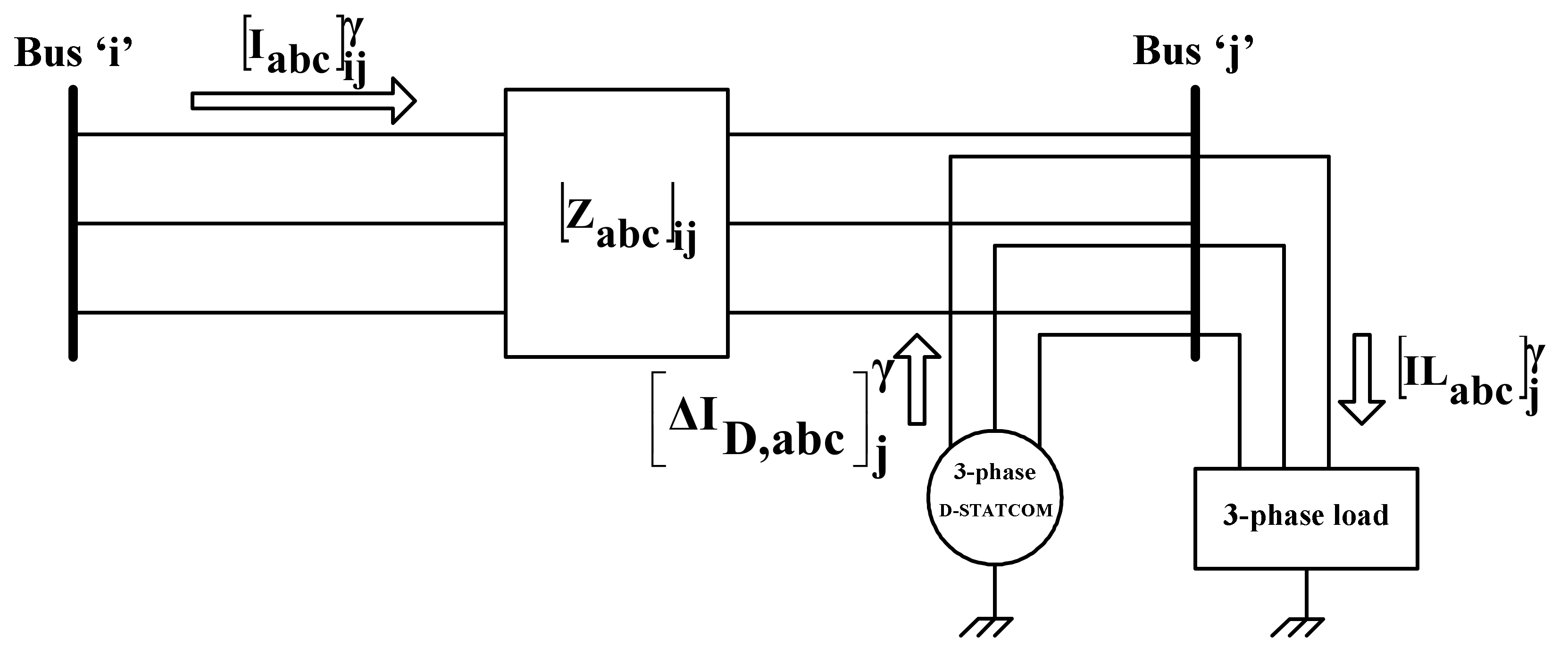
- In Figure 5, by applying the KCL at bus-j, the line current matrix in branch-ij is obtained as:With and , the reactive power flow in the line is evaluated. Then, the incremental reactive current injection matrix is obtained with Equation (20):The reactive power generation matrix needed at D-STATCOM bus-j is obtained with Equation (21):
- If the D-STATCOM device is able to generate limited reactive power, then find the total reactive power generation of D-STATCOM device with Equation (22). The total reactive power generation of D-STATCOM is now compared with the maximum and minimum limits of reactive power generation of D-STATCOM device limits. Equation (22) is calculated as follows:IfThen set complex power generation is as in Equation (21)IfThen set andIfThen set and
- Now, find the complex power generation matrix at D-STATCM bus with Equation (23):where is the specified real power generation matrix of the D-STATCOM device and its value is set to zero.
- The line current matrix injected by the D-STATCOM is obtained with the complex power generation matrix obtained in Equation (23) and bus voltage matrix as:
- Using the current injection matrix at the D-STATCOM buses, repeat from step 7 by setting γ = γ+1.
- If Equation (16) is satisfied at all D-STATCOM buses, then stop the FPFA algorithm.
- With the complex power loss in branch-ij in Equation (25), find the total power loss in the network by summing up the losses in all branches:
- 18.
- With the converged bus voltages and specified load, the impedances of the linear loads are calculated for the harmonic order-h of interest.
- 19.
- Find the harmonic current injection matrix for the non-linear loads for the selected h-order harmonic of interest. The harmonic current injection matrix of D-STATCOM is taken as zero.
- 20.
- The harmonic voltage at the substation bus is taken as zero since the supply voltage is assumed to bea pure sinusoidal voltage waveform.
- 21.
- The harmonic voltages at all other buses for the first iteration are assumed to be zeros as that of the substation bus:
- 22.
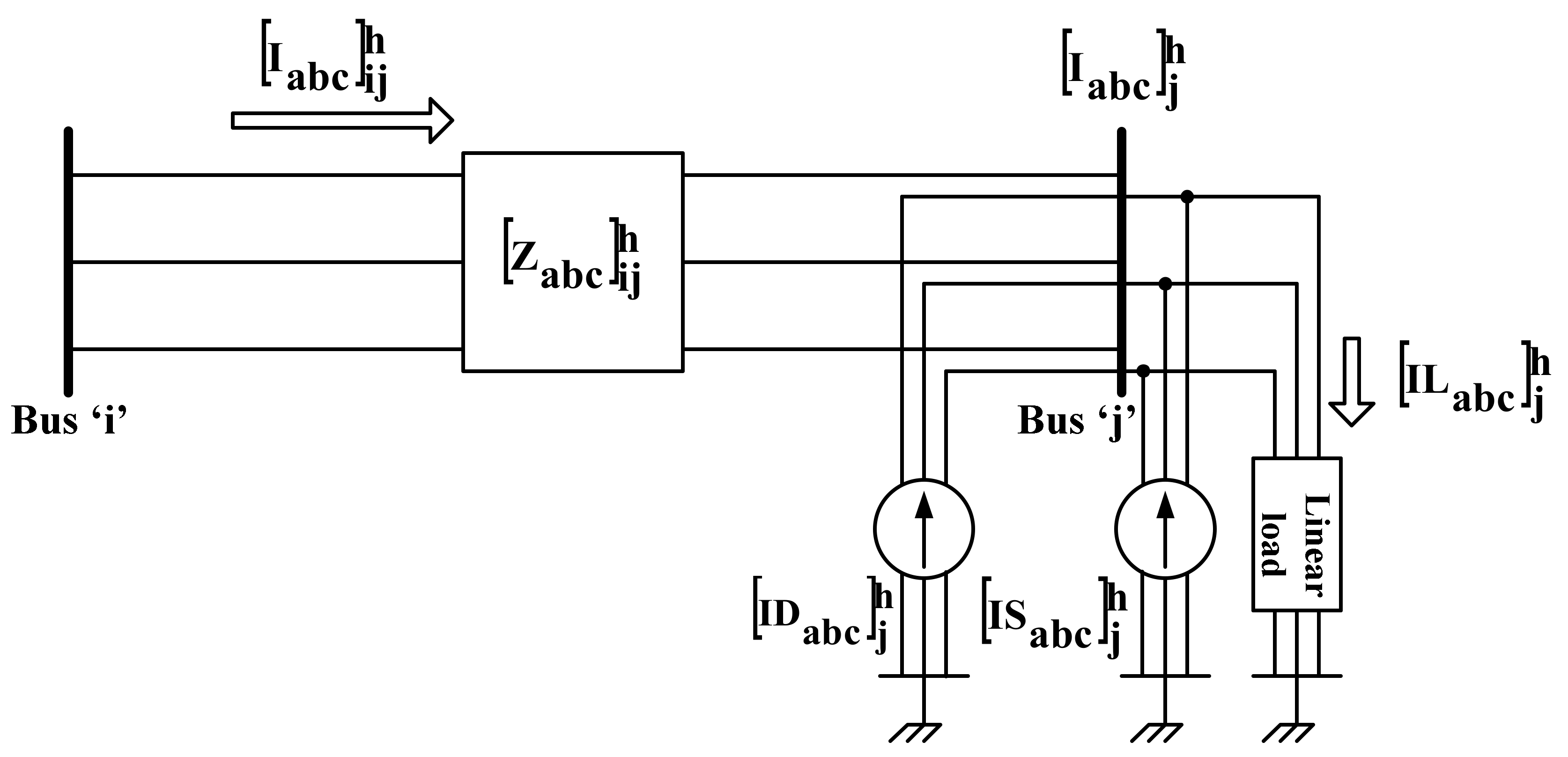
- Find the net harmonic current matrix at all the buses with the harmonic current matrix drawn by the linear loads and the harmonic current injection matrix of non-linear loads and the D-STATCOM device. The current matrix drawn by the linear loads at all the buses is zero for the first iteration as the harmonic voltage at all the buses is zero for the first iteration. This is illustrated with the sample section as shown in Figure 6. The net harmonic current matrix at bus-j is given by Equation (27), and the harmonic current matrix in branch-ij is given by Equation (28):where:Harmonic current matrix at bus-j for harmonic order-h;Harmonic current matrix in branch-ij for harmonic order-h;Harmonic current matrix drawn by linear load at bus-j for harmonic order-h;Harmonic current injection matrix by non-linear load at bus-j for harmonic order-h;Harmonic current injection matrix by D-STATCOM device at bus-j for harmonic order-h.Likewise, the harmonic currents in all branches are to be obtained by moving up to the substation as explained in step 3 to step 4 in PartA for FPFA.
- 23.
- Then, start finding the harmonic voltages at all buses downstream from the substation bus with Equation (29) as explained in step 5 in PartA:
- 24.
- Repeat the steps 22 to 23 until the magnitude mismatch of harmonic voltages of h-order at all the busses is within the tolerance limit.
- 25.
- Find the harmonic power loss in all branches using Equation (30). Then find the total harmonic power loss in the network for the selected harmonic order-h using Equation (31):
- 26.
- Likewise, repeat the steps from 10 to 16 for all the harmonics of selected harmonic orders (h = 3, 5, 7, 9, 11, 13, and 15).
- 27.
- Find the total harmonic loss of the network using Equation (32):
- 28.
- The total r.m.s voltage at bus-i, say, phase ‘a’, is calculated as:
- 29.
- The total harmonic distortion at every bus is calculated using Equation (34):where:Minimum harmonic order;
5. Results and Discussions
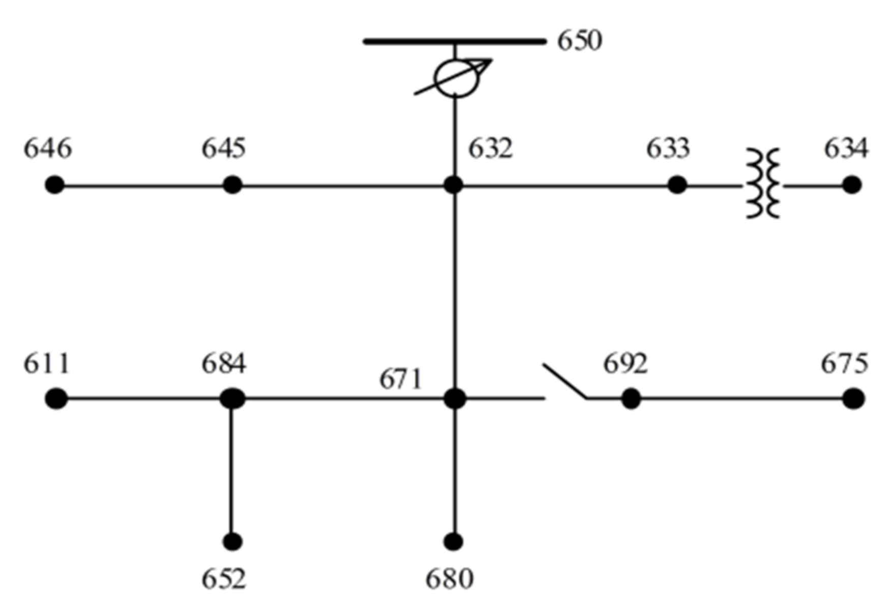
5.1. IEEE−13 Bus URDN
5.1.1. Fundamental Power Flow Solution for Accuracy Test
5.1.2. Fundamental and Harmonic Power Flow Solutions without D-STATCOM
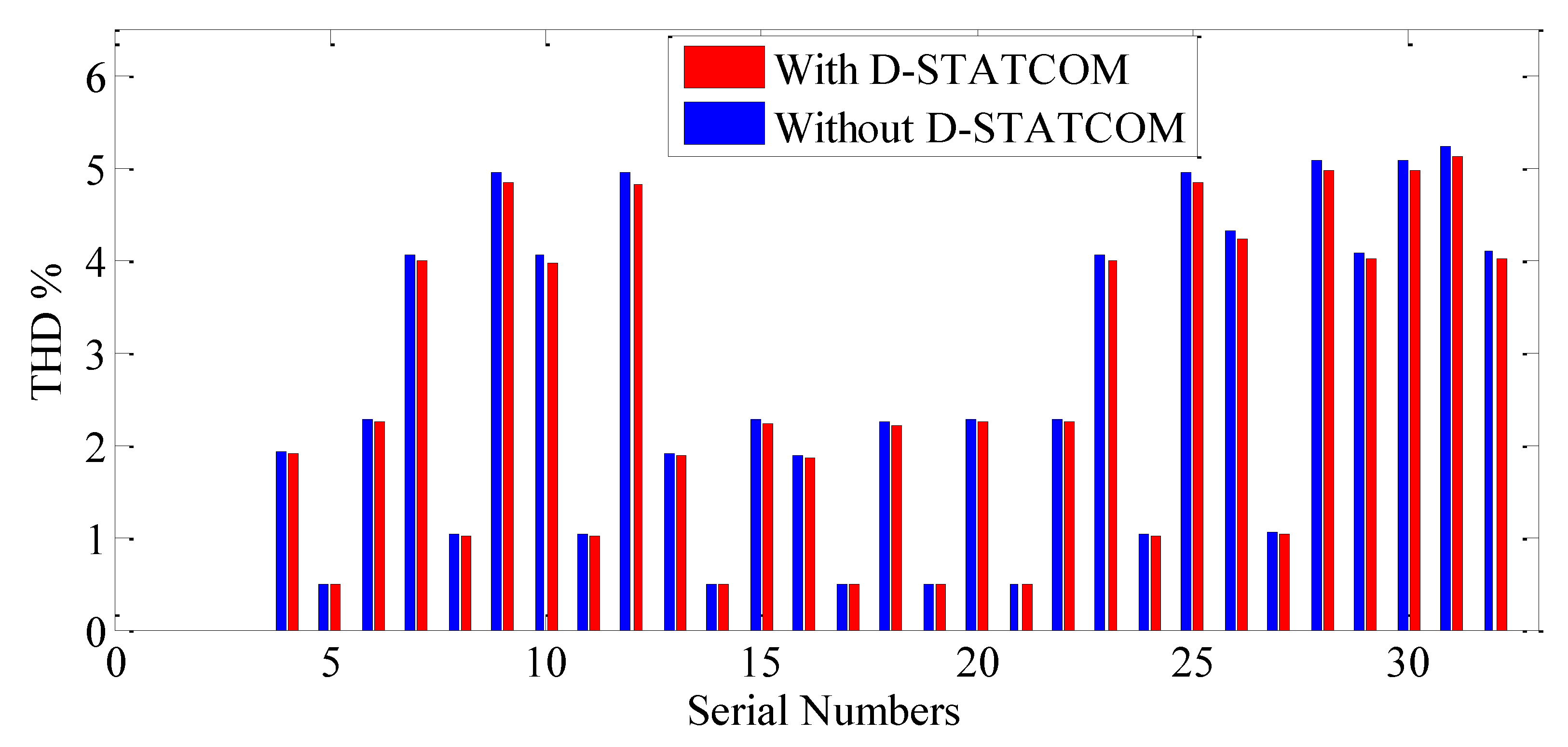
5.1.3. IEEE−13 Bus URDN with D-STATCOM
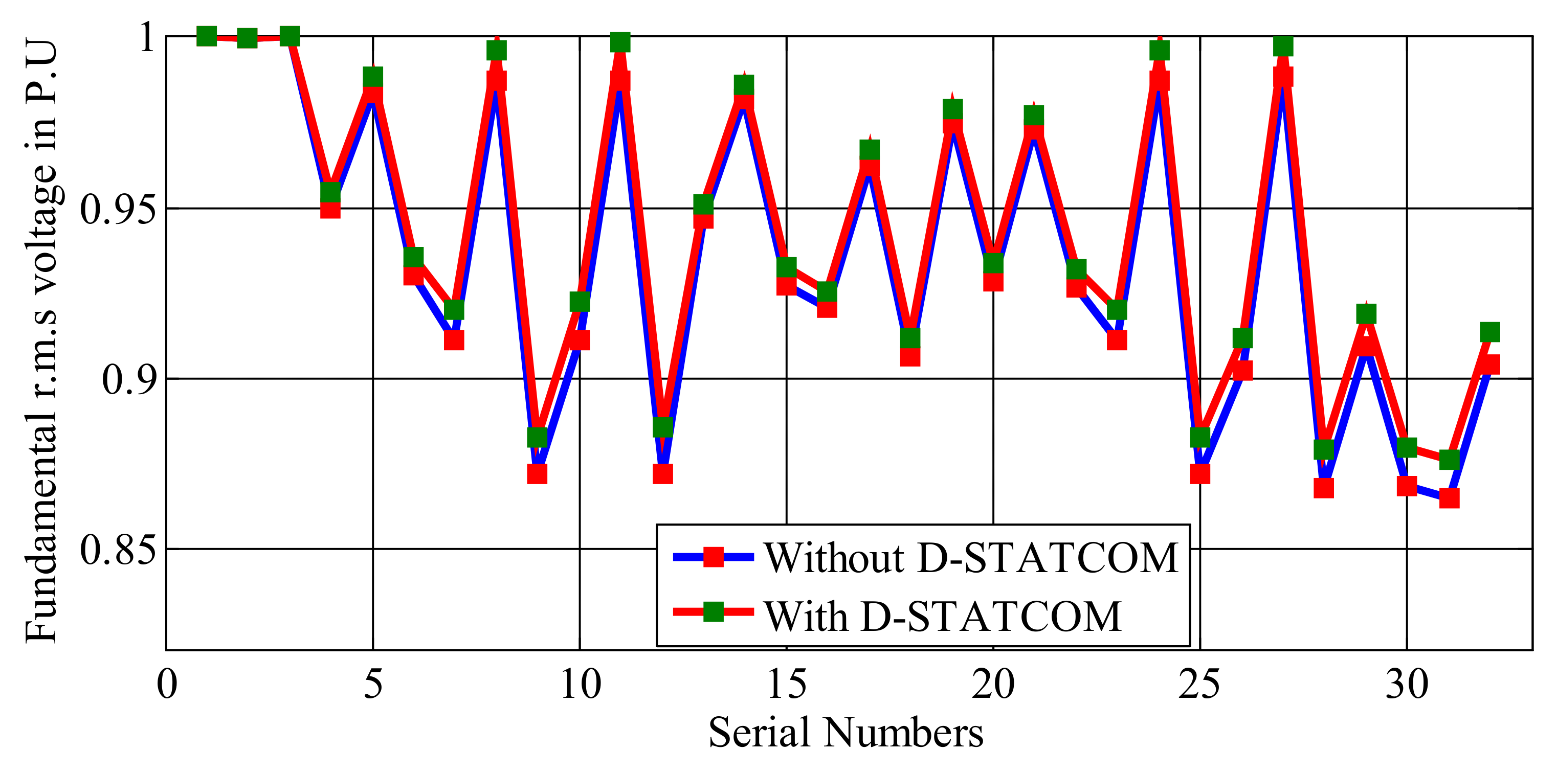
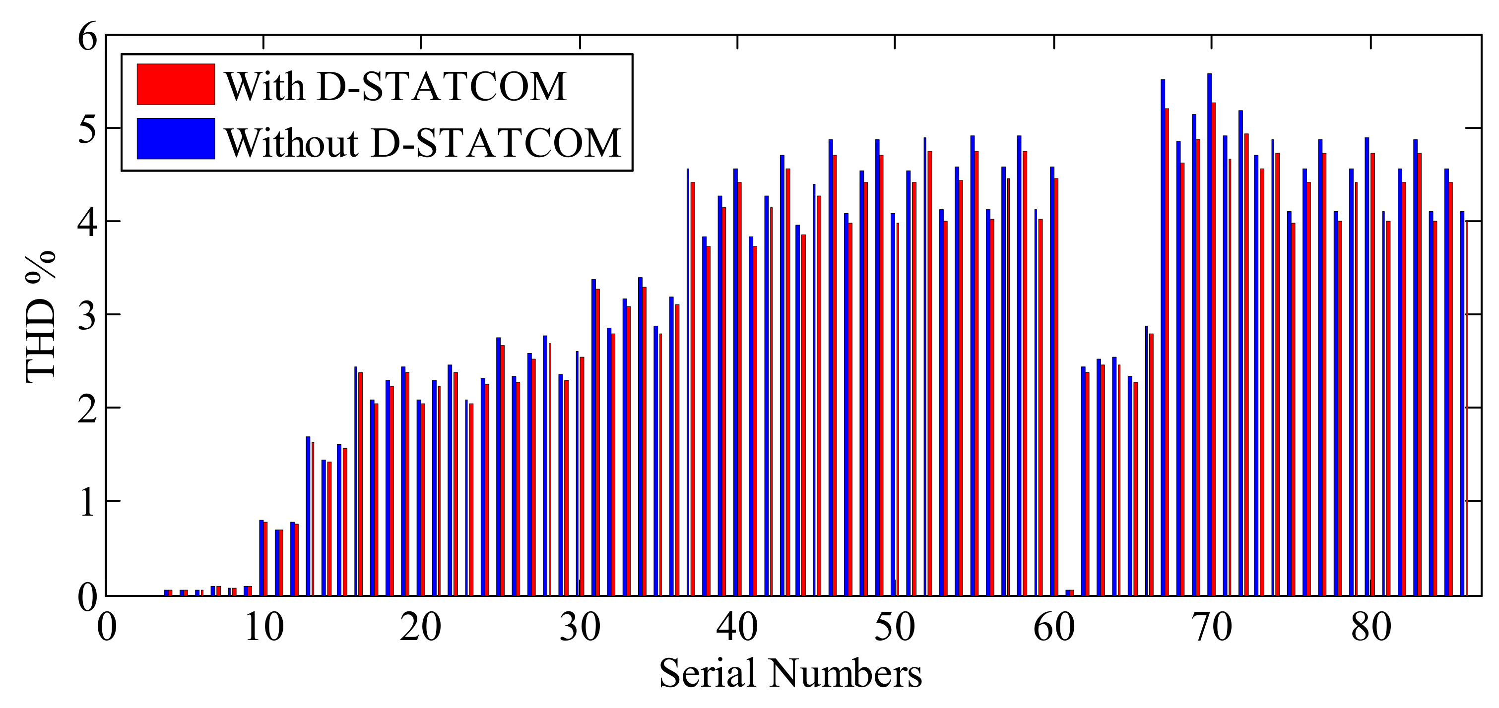
5.2. IEEE−34 Bus URDN
6. Conclusions
Author Contributions
Funding
Conflicts of Interest
References
- Burch, R.; Chang, G.K.; Grady, M.; Hatziadoniu, C.; Liu, Y.; Marz, M.; Ortmeyer, T.; Xu, W.; Ranade, S.; Ribeiro, P. Impact of aggregate linear load modeling on harmonic analysis: A comparison of common practice and analytical models. IEEETrans. Power Deliv. 2003, 18, 625–630. [Google Scholar] [CrossRef]
- Yang, N.-C.; Le, M.-D. Three-phase harmonic power flow by direct ZBUS method for unbalanced radial distribution systems with passive power filters. IET Gener. Transm. Distrib. 2016, 10, 3211–3219. [Google Scholar] [CrossRef]
- Milovanović, M.; Radosavljević, J.; Perović, B.; Dragičević, M. Power flow in radial distribution systems in the presence of harmonics. Int. J. Electr. Eng. Comput. 2018, 2, 11–19. [Google Scholar] [CrossRef]
- Amini, M.A.; Jalilian, A.; Behbahani, M.R.P. Fast network reconfiguration in harmonic polluted distribution network based on developed backward/forward sweep harmonic load flow. Electr. Power Syst. Res. 2019, 168, 295–304. [Google Scholar] [CrossRef]
- Milovanović, M.; Radosavljević, J.; Perović, B. A backward/forward sweep power flow method for harmonic polluted radial distribution systems with distributed generation units. Int. Trans. Electr. Energy Syst. 2019, 30, e12310. [Google Scholar] [CrossRef]
- Nduka, O.S.; Ahmadi, A.R. Data-driven robust extended computer-aided harmonic power flow analysis. IET Gener. Transm. Distrib. 2020, 14, 4398–4409. [Google Scholar] [CrossRef]
- Hernandez, J.C.; Ruiz-Rodriguez, F.J.; Jurado, F.; Sanchez-Sutil, F. Tracing harmonic distribution and voltage unbalance in secondary radial distribution networks with photovoltaic uncertainties by a multiphase harmonic load flow. Electr. Power Syst. Res. 2020, 185, 1–18. [Google Scholar] [CrossRef]
- Ruiz-Rodriguez, F.J.; Hernandez, J.C.; Jurado, F. Iterative harmonic load flow by using the point-estimate method and complex affine arithmetic for radial distribution systems with photovoltaic uncertainties. Electr. Power Energy Syst. 2020, 118, 1–16. [Google Scholar] [CrossRef]
- El-Fergany, A.; Abdelaziz, A.Y. Cuckoo Search-based Algorithm for Optimal Shunt Capacitors Allocations in Distribution Networks. Electr. Power Compon. Syst. 2013, 41, 1567–1581. [Google Scholar] [CrossRef]
- Abdelaziz, A.Y.; Ali, E.S.; Abd Elazim, S.M. Flower Pollination Algorithm for Optimal Capacitor Placement and Sizing in Distribution Systems. Electr. Power Compon. Syst. J. 2016, 44, 544–555. [Google Scholar] [CrossRef]
- Satish, R.; Kantarao, P.; Vaisakh, K. A new algorithm for impacts of multiple DGs and D-STATCOM in unbalanced radial distribution networks. Int. J. Renew. Energy Technol. 2021, 12, 221–242. [Google Scholar] [CrossRef]
- Satish, R.; Vaisakh, K.; Abdelaziz, A.Y.; El-Shahat, A. A Novel Three-phase Power Flow Algorithm for Evaluation of Impact of Renewable Energy Sources and D-STATCOM Device in Unbalanced Radial Distribution Networks. Energies 2021, 14, 6152. [Google Scholar] [CrossRef]
- Othman, M.M.; Hegazy, Y.G.; Abdelaziz, A.Y. Electrical Energy Management in Unbalanced Distribution Networks using Virtual Power Plant Concept. Electr. Power Syst. Res. 2017, 145, 157–165. [Google Scholar] [CrossRef]
- Abdelaziz, A.Y.; Hegazy, Y.G.; El-Khattam, W.; Othman, M.M. A Multi objective Optimization for Sizing and Placement of Voltage Controlled Distributed Generation Using Supervised Big Bang Big Crunch Method. Electr. Power Compon. Syst. 2015, 43, 105–117. [Google Scholar] [CrossRef]
- Abdelaziz, A.Y.; Hegazy, Y.G.; El-Khattam, W.; Othman, M.M. Optimal Planning of Distributed Generators in Distribution Networks Using Modified Firefly Method. Electr. Power Compon. Syst. 2015, 43, 320–333. [Google Scholar] [CrossRef]
- Rohouma, W.; Balog, R.S.; Peerzada, A.A.; Begovic, M.M. D-STATCOM for harmonic mitigation in low voltage distribution network with high penetration of nonlinear loads. Renew. Energy 2020, 145, 1449–1464. [Google Scholar] [CrossRef]
- Sirjani, R.; Jordehi, A.R. Optimal placement and sizing of distribution static compensator (D-STATCOM) in electric distribution networks: A review. Renew. Sustain. Energy Rev. 2017, 77, 688–694. [Google Scholar] [CrossRef]
- Rezaeian-Marjani, S.; Galvani, S.; Talavat, V.; Farhadi-Kangarlu, M. Optimal allocation of D-STATCOM in distribution networks including correlated renewable energy sources. Electr. Power Energy Syst. 2020, 122, 1–14. [Google Scholar] [CrossRef]
- Patel, S.K.; Arya, S.R.; Maurya, R. Optimal Step LMS-Based Control Algorithm for DSTATCOM in Distribution System. Electr. Power Compon. Syst. 2019, 47, 675–691. [Google Scholar] [CrossRef]
- Singh, B.; Singh, S. GA-based optimization for integration of DGs, STATCOM and PHEVs in distribution systems. Energy Rep. 2019, 5, 84–103. [Google Scholar] [CrossRef]
- Badoni, M.; Singh, A.; Singh, B.; Saxena, H. Real-time implementation of active shunt compensator with adaptive SRLMMN control technique for power quality improvement in the distribution system. Int. Trans. Electr. Energy Syst. 2020, 14, 1598–1606. [Google Scholar] [CrossRef]
- Selvaraj, G.; Rajangam, K. Multi-objective grey wolf optimizer algorithm for combination of network reconfiguration and D-STATCOM allocation in distribution system. Int. Trans. Electr. Energy Syst. 2019, 29, e12100. [Google Scholar] [CrossRef]
- Kersting, W.H. Distribution System Modeling and Analysis, 4th ed.; CRC Press: Boca Raton, FL, USA, 2017. [Google Scholar]
- Task Force on Harmonics Modeling and Simulation. Modeling and simulation of the propagation of harmonics in electric power networks I. Concepts, models, and simulation techniques. IEEE Trans. Power Deliv. 1996, 11, 452–465. [Google Scholar] [CrossRef]
- Chen, T.H.; Chang, J.D.; Chang, Y.L. Models of grounded mid-tap open-wye and open-delta connected transformers for rigorous analysis of a distribution system. IEEE Proc. Gener. Transm. Distrib. 1996, 143, 82–88. [Google Scholar] [CrossRef]
- Arrillaga, J.; Bradley, D.A.; Bodger, P.S. Power System Harmonics, 1st ed.; Wiley: Hoboken, NJ, USA, 1985. [Google Scholar]
- Yang, Z.; Shen, C.; Crow, M.L.; Zhang, L. An improved STATCOM model for power flow analysis. In Proceedings of the 2000 Power Engineering Society Summer Meeting, Seattle, WA, USA, 16–20 July 2000; pp. 1121–1126. [Google Scholar]
- Jazebi, S.; Hosseinian, S.H.; Vahidi, B. DSTATCOM allocation in distribution networks considering reconfiguration using differential evolution algorithm. Energy Convers. Manag. 2011, 52, 2777–2783. [Google Scholar] [CrossRef]
- Das, D.; Nagi, H.S.; Kothari, D.P. Novel method for solving radial distribution networks. IEEE Proc. Gener. Transm. Distrib. 1994, 141, 291–298. [Google Scholar] [CrossRef]
- Shirmohammadi, D.; Carol, S.; Cheng, A. A Three phase power flow method for real time distribution system analysis. IEEE Trans. Power Syst. 1995, 10, 671–679. [Google Scholar]
- Radial Distribution Test Feeders. Available online: http://sites.ieee.org/pes-testfeeders/resources (accessed on 28 September 2021).
- Abu-Hashim, R.; Burch, R.; Chang, G.; Grady, M.; Gunther, E.; Halpin, M.; Xu, W.; Marz, M.; Sim, T.; Liu, Y.; et al. Test systems for harmonic modeling and simulation. IEEE Trans. Power Deliv. 1999, 14, 579–587. [Google Scholar] [CrossRef]


| Wye Connection | Delta Connection | |
|---|---|---|
| Phase voltage matrix and specified load matrix at bus. | , | , |
| Phase current matrix serving constant power load | ||
| Phase current matrix serving the constant impedance load | ||
| Phase current matrix serving the constant current load | ||
| Line current matrix entering the load | ||
| Distributed Loads | Create a duplicate node at a distance of one-fourth the length from the sending end and connect a two-third of lode. At the receiving end one-third of load is connected. | |
| Wye Connected | Delta Connected | |
|---|---|---|
| Phase voltage matrix and specified reactive power matrix at bus. | , | , |
| Phase current matrix serving the capacitor bank | ||
| Line current matrix serving the capacitor bank |
| Branch Number(BN) | Sending Bus(SE) | Receiving Bus(RE) |
|---|---|---|
| 1 | 1 | 2 |
| 2 | 2 | 3 |
| 3 | 3 | 4 |
| 4 | 4 | 5 |
| 5 | 5 | 6 |
| 6 | 6 | 7 |
| 7 | 7 | 8 |
| 8 | 8 | 9 |
| 9 | 9 | 10 |
| 10 | 10 | 11 |
| 11 | 3 | 12 |
| 12 | 12 | 13 |
| 13 | 13 | 14 |
| 14 | 14 | 15 |
| 15 | 15 | 16 |
| 16 | 6 | 17 |
| 17 | 17 | 18 |
| 18 | 18 | 19 |
| 19 | 19 | 20 |
| 20 | 20 | 21 |
| 21 | 18 | 22 |
| 22 | 22 | 23 |
| Bus | Phase | Obtained Solution | IEEE Solution [31] | Error in Voltage Mag. | Error in Voltage Ang. |
|---|---|---|---|---|---|
| 650 | a | 1 0o | 1 0o | 0.0000 | 0.00 |
| b | 1 −120o | 1 −120o | 0.0000 | 0.00 | |
| c | 1 120o | 1 120o | 0.0000 | 0.00 | |
| RG | a | 1.0625 0o | 1.0625 0o | 0.0000 | 0.00 |
| b | 1.0500 −120o | 1.0500 −120o | 0.0000 | 0.00 | |
| c | 1.0687 120o | 1.0687 120o | 0.0000 | 0.00 | |
| 632 | a | 1.0210 −2.49o | 1.0210 −2.49o | 0.0000 | 0.00 |
| b | 1.0420 −121.72o | 1.0420 −121.72o | 0.0000 | 0.00 | |
| c | 1.0175 117.83o | 1.0170 117.83o | −0.0005 | 0.00 | |
| 671 | a | 0.9900 −5.30o | 0.9900 −5.30o | 0.0000 | 0.00 |
| b | 1.0529 −122.34o | 1.0529 −122.34o | 0.0000 | 0.00 | |
| c | 0.977 116.03o | 0.9778 116.02o | 0.0001 | −0.01 | |
| 680 | a | 0.9900 −5.30o | 0.9900 −5.30o | 0.0000 | 0.00 |
| b | 1.0529 −122.34o | 1.0529 −122.34o | 0.0000 | 0.00 | |
| c | 0.9778 116.03o | 0.977 116.02o | 0.0001 | −0.01 | |
| 633 | a | 1.0180 −2.55o | 1.0180 −2.56o | 0.0000 | 0.01 |
| b | 1.0401 −121.77o | 1.0401 −121.77o | 0.0000 | 0.00 | |
| c | 1.0148 117.82o | 1.0148 117.82o | 0.0000 | 0.00 | |
| 634 | a | 0.9940 −3.23o | 0.9940 −3.23o | 0.0000 | 0.00 |
| b | 1.0218 −122.22o | 1.0218 −122.22o | 0.0000 | 0.00 | |
| c | 0.9960 117.35o | 0.9960 117.34o | 0.0000 | −0.01 | |
| 645 | b | 1.0328 −121.90o | 1.0329 −121.90o | 0.0001 | 0.00 |
| c | 1.0155 117.86o | 1.0155 117.86o | 0.0001 | 0.00 | |
| 646 | b | 1.0311 −121.98o | 1.0311 −121.98o | 0.0000 | 0.00 |
| c | 1.0134 117.90o | 1.0134 117.90o | 0.0000 | 0.01 | |
| 692 | a | 0.9900 −5.30o | 0.9900 −5.31o | 0.0000 | 0.01 |
| b | 1.0529 −122.34o | 1.0529 −122.34o | 0.0000 | 0.00 | |
| c | 0.9778 116.03o | 0.9777 116.02o | −0.0001 | −0.01 | |
| 675 | a | 0.9835 −5.55o | 0.9835 −5.56o | 0.0000 | 0.01 |
| b | 1.0553 −122.52o | 1.0553 −122.52o | 0.0000 | 0.00 | |
| c | 0.9759 116.04o | 0.9758 116.03o | −0.0001 | −0.01 | |
| 684 | a | 0.9881 −5.32o | 0.9881 −5.32o | 0.0000 | 0.00 |
| c | 0.9758 115.92o | 0.9758 115.92o | 0.0000 | 0.00 | |
| 611 | c | 0.9738 115.78o | 0.9738 115.78o | 0.0000 | 0.00 |
| 652 | a | 0.9825 −5.24o | 0.9825 −5.25o | 0.0000 | 0.01 |
| Phase | Obtained Power Loss | IEEE Loss [31] | ||
|---|---|---|---|---|
| Active (kW) | Reactive (kVAR) | Active (kW) | Reactive (kVAR) | |
| a | 39.13 | 152.62 | 39.11 | 152.59 |
| b | −4.74 | 42.27 | −4.70 | 42.22 |
| c | 76.59 | 129.69 | 76.65 | 129.85 |
| Total | 110.98 | 324.57 | 111.13 | 324.66 |
| Harmonic Order | Harmonic Power Loss | |
|---|---|---|
| APL (kW) | RPL (kVAR) | |
| 3 | 0.7958 | 6.5165 |
| 5 | 0.0856 | 1.1483 |
| 7 | 0.0072 | 0.1183 |
| 9 | 0.0043 | 0.0902 |
| 11 | 0.0008 | 0.0164 |
| 13 | 0.0008 | 0.0226 |
| 15 | 0.0010 | 0.0340 |
| Total harmonic loss | 0.8983 | 7.9464 |
| Fundamental loss | 147.33 | 433.54 |
| Total power loss | 148.23 | 441.49 |
| Bus | Phase | S. No | Fundamental r.m.s Voltage | Total r.m.s Voltage | THD % |
|---|---|---|---|---|---|
| 650 | a | 1 | 1 0o | 1 | 0 |
| b | 2 | 1 −120o | 1 | 0 | |
| c | 3 | 1 120o | 1 | 0 | |
| 632 | a | 4 | 0.9498 −2.7462o | 0.9500 | 1.9173 |
| b | 5 | 0.9839 −121.6817o | 0.9839 | 0.4974 | |
| c | 6 | 0.9300 117.8000o | 0.9302 | 2.2737 | |
| 671 | a | 7 | 0.9109 −5.8987o | 0.9117 | 4.0623 |
| b | 8 | 0.9875 −122.2091o | 0.9875 | 1.0363 | |
| c | 9 | 0.8717 115.9500o | 0.8728 | 4.9409 | |
| 680 | a | 10 | 0.9109 −5.8987o | 0.9117 | 4.0623 |
| b | 11 | 0.9875 −122.2091o | 0.9875 | 1.0363 | |
| c | 12 | 0.8717 115.9500o | 0.8728 | 4.9409 | |
| 633 | a | 13 | 0.9466 −2.8223o | 0.9468 | 1.9098 |
| b | 14 | 0.9819 −121.7315o | 0.9819 | 0.4919 | |
| c | 15 | 0.9271 117.7946o | 0.9273 | 2.2648 | |
| 634 | a | 16 | 0.9207 −3.6073o | 0.9209 | 1.8801 |
| b | 17 | 0.9624 −122.2445o | 0.9624 | 0.4873 | |
| c | 18 | 0.9064 117.2178o | 0.9066 | 2.2406 | |
| 645 | b | 19 | 0.9745 −121.8646o | 0.9745 | 0.4991 |
| c | 20 | 0.9283 117.8225o | 0.9286 | 2.2769 | |
| 646 | b | 21 | 0.9729 −121.9382o | 0.9729 | 0.5000 |
| c | 22 | 0.9264 117.8696o | 0.9267 | 2.2815 | |
| 692 | a | 23 | 0.9109 −5.8987o | 0.9117 | 4.0623 |
| b | 24 | 0.9875 −122.2091o | 0.9875 | 1.0363 | |
| c | 25 | 0.8717 115.9500o | 0.8728 | 4.9409 | |
| 675 | a | 26 | 0.9025 −6.0795o | 0.9034 | 4.3128 |
| b | 27 | 0.9887 −122.3037o | 0.9887 | 1.0491 | |
| c | 28 | 0.8678 116.0660o | 0.8689 | 5.0687 | |
| 684 | a | 29 | 0.9093 −5.9502o | 0.9100 | 4.0765 |
| c | 30 | 0.8684 115.9163o | 0.8695 | 5.0741 | |
| 611 | c | 31 | 0.8651 115.8365o | 0.8663 | 5.2263 |
| 652 | a | 32 | 0.9041 −5.8755o | 0.9049 | 4.0900 |
| Harmonic Order | Harmonic Power Loss | |
|---|---|---|
| Active (kW) | Reactive (kVAR) | |
| 3 | 0.7836 | 6.3935 |
| 5 | 0.0841 | 1.1282 |
| 7 | 0.0071 | 0.1168 |
| 9 | 0.0043 | 0.0886 |
| 11 | 0.0008 | 0.0160 |
| 13 | 0.0008 | 0.0223 |
| 15 | 0.0009 | 0.0336 |
| Total harmonic loss | 0.8816 | 7.7991 |
| Fundamental Loss | 135.34 | 396.63 |
| Total power loss | 136.22 | 404.43 |
| Bus | Phase | Fundamental r.m.s Voltage | Total r.m.s Voltage in p.u | THD % |
|---|---|---|---|---|
| 650 | a | 1.00000o | 1 | 0 |
| b | 1.0000−120o | 1 | 0 | |
| c | 1.0000120o | 1 | 0 | |
| 632 | a | 0.9545−2.8433o | 0.9547 | 1.8920 |
| b | 0.9883−121.7039o | 0.9883 | 0.4923 | |
| c | 0.9355117.6975o | 0.9357 | 2.2404 | |
| 671 | a | 0.9204−6.0689o | 0.9211 | 3.9865 |
| b | 0.9961−122.2496o | 0.9962 | 1.0211 | |
| c | 0.8829115.7512o | 0.8839 | 4.8346 | |
| 680 | a | 0.9227−6.1274o | 0.9234 | 3.9764 |
| b | 0.9983−122.2605o | 0.9983 | 1.0189 | |
| c | 0.8855115.6856o | 0.8865 | 4.8205 | |
| 633 | a | 0.9512−2.9186o | 0.9514 | 1.8846 |
| b | 0.9863−121.7535o | 0.9863 | 0.4869 | |
| c | 0.9326117.6923o | 0.9329 | 2.2317 | |
| 634 | a | 0.9255−3.6957o | 0.9256 | 1.8556 |
| b | 0.9669−122.2618o | 0.9669 | 0.4823 | |
| c | 0.9121117.1225o | 0.9123 | 2.2082 | |
| 645 | b | 0.9789−121.8864o | 0.9789 | 0.4940 |
| c | 0.9338117.7205o | 0.9341 | 2.2436 | |
| 646 | b | 0.9773−121.9600o | 0.9773 | 0.4948 |
| c | 0.9319117.7674o | 0.9322 | 2.2482 | |
| 692 | a | 0.9204−6.0689o | 0.9211 | 3.9865 |
| b | 0.9961−122.2496o | 0.9962 | 1.0211 | |
| c | 0.8829115.7512o | 0.8839 | 4.8346 | |
| 675 | a | 0.9121−6.2456o | 0.9129 | 4.2312 |
| b | 0.9973−122.3429o | 0.9973 | 1.0335 | |
| c | 0.8790115.8645o | 0.8801 | 4.9586 | |
| 684 | a | 0.9187−6.1203o | 0.9194 | 4.0007 |
| c | 0.8796115.7184o | 0.8807 | 4.9647 | |
| 611 | c | 0.8763115.6396o | 0.8775 | 5.1133 |
| 652 | a | 0.9135−6.0456o | 0.9142 | 4.0140 |
| Bus No. | Load Composition | |||
|---|---|---|---|---|
| Non-Linear Loads | Linear Loads | |||
| Fluorescent Light Banks | Adjustable Speed Drives | Composite Residential Loads | ||
| 830 | None | None | 80% | 20% |
| 844 | 30% | 30% | 30% | 10% |
| 848 | 30% | 30% | 30% | 10% |
| 890 | 30% | None | 60% | 10% |
| 860 | 30% | 30% | 30% | 10% |
| 840 | 30% | 30% | 30% | 10% |
| Case Study | Description |
|---|---|
| Case 1 (Without D-STATCOM) |
|
| Case 2 (With D-STATCOM) |
|
| Bus No. | S. No. | Ph. | Total r.m.s Voltages in p.u | THD % | Bus No | S. No. | Ph. | Total r.m.sVoltages in p.u | THD % |
|---|---|---|---|---|---|---|---|---|---|
| 800 | 1 | a | 1 | 0 | 46 | a | 0.8169 | 4.8628 | |
| 2 | b | 1 | 0 | 834 | 47 | b | 0.8531 | 4.0835 | |
| 3 | c | 1 | 0 | 48 | c | 0.8570 | 4.5399 | ||
| 802 | 4 | a | 0.9972 | 0.0541 | 49 | a | 0.8168 | 4.8691 | |
| 5 | b | 0.9980 | 0.0481 | 842 | 50 | b | 0.8530 | 4.0888 | |
| 6 | c | 0.9981 | 0.0531 | 51 | c | 0.8569 | 4.5458 | ||
| 806 | 7 | a | 0.9953 | 0.0908 | 52 | a | 0.8164 | 4.8990 | |
| 8 | b | 0.9967 | 0.0808 | 844 | 53 | b | 0.8524 | 4.1147 | |
| 9 | c | 0.9969 | 0.0891 | 54 | c | 0.8565 | 4.5742 | ||
| 808 | 10 | a | 0.9605 | 0.7955 | 55 | a | 0.8162 | 4.9094 | |
| 11 | b | 0.9745 | 0.6983 | 846 | 56 | b | 0.8519 | 4.1261 | |
| 12 | c | 0.9742 | 0.7706 | 57 | c | 0.8562 | 4.5841 | ||
| 812 | 13 | a | 0.9200 | 1.6825 | 58 | a | 0.8162 | 4.9109 | |
| 14 | b | 0.9488 | 1.4531 | 848 | 59 | b | 0.8518 | 4.1276 | |
| 15 | c | 0.9479 | 1.6045 | 60 | c | 0.8562 | 4.5855 | ||
| 814 | 16 | a | 0.8880 | 2.4435 | 810 | 61 | b | 0.9975 | 0.0562 |
| 17 | b | 0.9284 | 2.0813 | 818 | 62 | a | 0.8869 | 2.4466 | |
| 18 | c | 0.9271 | 2.2994 | 820 | 63 | a | 0.8599 | 2.5235 | |
| 850 | 19 | a | 0.8880 | 2.4438 | 822 | 64 | a | 0.8564 | 2.5339 |
| 20 | b | 0.9284 | 2.0815 | 826 | 65 | b | 0.9169 | 2.3333 | |
| 21 | c | 0.9271 | 2.2997 | 856 | 66 | b | 0.8954 | 2.8693 | |
| 816 | 22 | a | 0.8877 | 2.4526 | 67 | a | 0.7875 | 5.5150 | |
| 23 | b | 0.9281 | 2.0888 | 888 | 68 | b | 0.8248 | 4.8565 | |
| 24 | c | 0.9268 | 2.3079 | 69 | c | 0.8275 | 5.1312 | ||
| 824 | 25 | a | 0.8778 | 2.7468 | 70 | a | 0.7853 | 5.5791 | |
| 26 | b | 0.9171 | 2.3328 | 890 | 71 | b | 0.8228 | 4.9085 | |
| 27 | c | 0.9173 | 2.5798 | 72 | c | 0.8252 | 5.1873 | ||
| 828 | 28 | a | 0.8769 | 2.7713 | 864 | 73 | a | 0.8203 | 4.7018 |
| 29 | b | 0.9162 | 2.3529 | 860 | 74 | a | 0.8164 | 4.8734 | |
| 30 | c | 0.9165 | 2.6025 | 75 | b | 0.8526 | 4.0921 | ||
| 830 | 31 | a | 0.8574 | 3.3823 | 76 | c | 0.8566 | 4.5493 | |
| 32 | b | 0.8961 | 2.8557 | 77 | a | 0.8162 | 4.8779 | ||
| 33 | c | 0.8974 | 3.1673 | 836 | 78 | b | 0.8522 | 4.0967 | |
| 854 | 34 | a | 0.8569 | 3.3981 | 79 | c | 0.8565 | 4.5531 | |
| 35 | b | 0.8956 | 2.8688 | 80 | a | 0.8162 | 4.8790 | ||
| 36 | c | 0.8969 | 3.1820 | 840 | 81 | b | 0.8522 | 4.0976 | |
| 852 | 37 | a | 0.8233 | 4.5667 | 82 | c | 0.8564 | 4.5542 | |
| 38 | b | 0.8603 | 3.8340 | 83 | a | 0.8162 | 4.8779 | ||
| 39 | c | 0.8634 | 4.2626 | 862 | 84 | b | 0.8522 | 4.0968 | |
| 832 | 40 | a | 0.8233 | 4.5671 | 85 | c | 0.8565 | 4.5530 | |
| 41 | b | 0.8603 | 3.8342 | 838 | 86 | b | 0.8520 | 4.0977 | |
| 42 | c | 0.8634 | 4.2629 | --- | |||||
| 858 | 43 | a | 0.8203 | 4.7018 | |||||
| 44 | b | 0.8570 | 3.9475 | ||||||
| 45 | c | 0.8604 | 4.3890 | ||||||
| Case Study | Min. Fundamental Voltage, p.u | Min. Total r.m.sVoltage, p.u | Max. THD% | No. of Phases of Buses (THD > 5%) |
|---|---|---|---|---|
| Case 1 | 0.7841 at bus−890, a-phase | 0.7853 at bus−890, a-phase | 5.5791 at bus−890, a-phase | 4 |
| Case 2 | 0.8137 at bus−890, a-phase | 0.8148 at bus−890, a-phase | 5.2567 at bus−890, a-phase | 2 |
| Case study | Total fundamental power loss | Total power loss including total harmonic loss | ||
| Active (kW) | Reactive (kVAR) | Active (kW) | Reactive (kVAR) | |
| Case 1 | 260.89 | 180.49 | 264.56 | 188.15 |
| Case 2 | 227.69 | 155.82 | 231.23 | 163.21 |
Publisher’s Note: MDPI stays neutral with regard to jurisdictional claims in published maps and institutional affiliations. |
© 2021 by the authors. Licensee MDPI, Basel, Switzerland. This article is an open access article distributed under the terms and conditions of the Creative Commons Attribution (CC BY) license (https://creativecommons.org/licenses/by/4.0/).
Share and Cite
Satish, R.; Vaisakh, K.; Abdelaziz, A.Y.; El-Shahat, A. A Novel Three-Phase Harmonic Power Flow Algorithm for Unbalanced Radial Distribution Networks with the Presence of D-STATCOM Devices. Electronics 2021, 10, 2663. https://doi.org/10.3390/electronics10212663
Satish R, Vaisakh K, Abdelaziz AY, El-Shahat A. A Novel Three-Phase Harmonic Power Flow Algorithm for Unbalanced Radial Distribution Networks with the Presence of D-STATCOM Devices. Electronics. 2021; 10(21):2663. https://doi.org/10.3390/electronics10212663
Chicago/Turabian StyleSatish, Raavi, Kanchapogu Vaisakh, Almoataz Y. Abdelaziz, and Adel El-Shahat. 2021. "A Novel Three-Phase Harmonic Power Flow Algorithm for Unbalanced Radial Distribution Networks with the Presence of D-STATCOM Devices" Electronics 10, no. 21: 2663. https://doi.org/10.3390/electronics10212663
APA StyleSatish, R., Vaisakh, K., Abdelaziz, A. Y., & El-Shahat, A. (2021). A Novel Three-Phase Harmonic Power Flow Algorithm for Unbalanced Radial Distribution Networks with the Presence of D-STATCOM Devices. Electronics, 10(21), 2663. https://doi.org/10.3390/electronics10212663