Abstract
In recent years, Environmental Sound Recognition (ESR) has become a relevant capability for urban monitoring applications. The techniques for automated sound recognition often rely on machine learning approaches, which have increased in complexity in order to achieve higher accuracy. Nonetheless, such machine learning techniques often have to be deployed on resource and power-constrained embedded devices, which has become a challenge with the adoption of deep learning approaches based on Convolutional Neural Networks (CNNs). Field-Programmable Gate Arrays (FPGAs) are power efficient and highly suitable for computationally intensive algorithms like CNNs. By fully exploiting their parallel nature, they have the potential to accelerate the inference time as compared to other embedded devices. Similarly, dedicated architectures to accelerate Artificial Intelligence (AI) such as Tensor Processing Units (TPUs) promise to deliver high accuracy while achieving high performance. In this work, we evaluate existing tool flows to deploy CNN models on FPGAs as well as on TPU platforms. We propose and adjust several CNN-based sound classifiers to be embedded on such hardware accelerators. The results demonstrate the maturity of the existing tools and how FPGAs can be exploited to outperform TPUs.
1. Introduction
Environmental Sound Recognition (ESR), especially in urban environments, is becoming a relevant feature for many applications, from monitoring traffic in smart cities [1] and monitoring criminal activity [2], to noise disturbances monitoring in residential or natural areas [3,4], such as the noise produced by overflying airplanes taking off or landing at a nearby airport [5]. Embedded platforms are often used toward the deployment of intelligent sound monitoring devices. Several methods have been explored in the past to accurately classify urban sounds using constrained embedded devices. Among others, k-Nearest Neighbor (k-NN), Support Vector Machine (SVM), Naive Bayes and Decision Trees are machine learning algorithms that have been already evaluated [6]. Recent advances in machine learning show that Deep Neural Networks (DNN), and more specifically, Convolutional Neural Networks (CNNs), provide high accuracy for sound recognition [7]. However, they often demand computationally intensive operations, with the consequence of having a limited accuracy and slow response time when ported to embedded devices. Recording sound locally with a microphone and processing it in the cloud is not always possible nor desirable. This approach cannot only introduce privacy concerns as the communication can be intercepted by a third party, but also leads to a high latency. Moreover, power consumption is also an important factor since most embedded devices are battery powered and designed for applications with a low complexity. High speed communication protocols are power consuming, and low power communication protocols have a low throughput, hence they are not real-time. Therefore, near-sensor intelligence or embedded solutions are necessary, ideally combining the accuracy of CNNs with high inference speed and low power consumption.
Dedicated platforms for this task already exist [8]. Google, for example, offers an extension to their popular machine learning framework, TensorFlow, for fast and lightweight CNN inference on high-level embedded platforms such as a Raspberry Pi (RPi). They also developed a dedicated Tensor Processing Unit (TPU) that serves as a hardware accelerator for deep neural networks and can be deployed as a low-latency, low-power embedded solution.
Field-Programmable Gate Arrays (FPGAs) are power efficient and highly suitable for computationally intensive algorithms like CNNs. Due to their parallel nature, they have the potential to accelerate the inference time compared to other embedded devices. Additionally, FPGAs can be configured to embed streaming architectures, leading to low-latency response solutions. Embedding a neural network on an FPGA is a time-consuming and high-effort task. Fortunately, several tool flows have recently been developed to allow the conversion of a CNN model from a high-level machine learning framework to one that is deployable for FPGAs.
The presented work evaluates the existing solutions for deploying CNN models on embedded devices. As an example, two CNN models for ESR are embedded. Due to the application requirements, low latency, power efficiency and real-time response, low-end FPGAs and TPUs are the embedded devices under evaluation, while high-end general-purpose embedded devices such as RPi are used as reference. Hardware accelerators such as FPGAs or TPUs are evaluated from the accuracy and latency perspective, while several tool flows are analyzed, evaluated and discussed. This includes the tool flows designed for embedding CNN models on FPGAs, hls4ml [9] and Vitis AI [10], as well as tool flows used for TPUs: Edge TPU [11] and TensorFlow Lite (TFLite) [12]. Altogether, this provides a wide perspective of the steps needed to follow and the effort expended toward embedding CNN models on FPGAs and TPUs, including the different strategies adopted to exploit such different technologies.
The main contributions of this work can be summarized as follows:
- Novel CNN model toward real-time ESR using hardware accelerators.
- In depth analysis, evaluation and discussion about the current tool flows for deploying CNN models on FPGAs and TPUs.
- Comparison of the achievable performance on FPGAs and TPUs for ESR for the novel CNN model and an adapted one.
This paper is organized as follows. Section 2 presents related work. The datasets and audio features used by the CNN models are described in Section 3. All of the background needed to understand the implemented CNN models, the evaluation of the generated solutions, tool flows and the description of the embedded platforms under test are described in Section 4. In Section 5, the novel CNN model is proposed and used to introduce, evaluate and discuss the hls4ml tool flow. The first experimental evaluation of the FPGA solutions and the TPU-based technologies is also presented. In Section 6, a second CNN model is adjusted to fully exploit the TPU characteristics and to evaluate the Vitis AI tool flow. The discussion of the experimental results and the lessons learned is contained in Section 7. Finally, the conclusions are drawn in Section 8.
2. Related Work
Previous works evaluated the use of machine learning techniques for sound recognition on embedded devices. For instance, in [6], several classical machine learning algorithms are embedded on a RPi, evaluated in terms of accuracy and classification time. Additionally, a hierarchical approach is presented to classify the audio in multiple stages, resulting in a more flexible solution by choosing the classifier in each stage, according to the type of audio and by considering execution time and power consumption.
The work presented in [7] is one of the earlier works that evaluate the use of CNNs for ESR. It has become a popular reference for newer networks to compare their performance using the ESC dataset [13].
The authors of [14] propose a real-time system for urban sound classification in an Internet of Things (IoT) context. Their CNN model is based on 2D convolutions using spectrogram feature maps as input and deployed on a RPi 4. However an evaluation concerning inference time is not presented. Similarly, in [15], another embedded solution making use of CNNs and spectrogram inputs is presented and evaluated. In this case, the classification happens on a low-power microcontroller. Multiple CNNs are compared to see which performs best with regard to accuracy in combination with CPU and memory usage of the microcontroller. Here, the timing summary is also missing. It shows however that lightweight CNNs for constrained embedded devices can still reach state-of-the-art accuracy.
An overview of the status, vision and challenges of the Internet of Audio Things (IoAuT) is given in [16], where the authors also tackle the challenges related to embedded machine learning for audio recognition and embedded solutions. Both pruning and quantization are proposed as methods for model compression when targeting deployment of an urban sound classification model in a constrained IoT context.
In [17,18,19], model compression methods for reducing resource consumption in hardware accelerators are presented. In fact, a framework is presented to modify CNNs for efficient inference on FPGAs by pruning weights from resource consuming layers. Similarly, an extension to prune neural networks for compression in TensorFlow [20] is evaluated in [18]. A tool for low-precision quantization is presented in [19]. These methods are used later in this work to compress and prepare CNN models for the FPGA.
The performance, architectural properties and supported deep learning frameworks of existing tool flows to embed CNNs on FPGAs are compared in [21]. A distinction is made between streaming architectures, where each layer is implemented as a single functional block, and single computational engine architectures, where all operations are executed sequentially using a specific DNN instruction set. This work aims for a streaming architecture, because of its advantages in throughput and its parallel potential on an FPGA.
In [9,22], the hls4ml, tool and tool flow is presented. This tool makes use of all previously mentioned techniques to compress a neural network for deployment in a streaming architecture on FPGAs. The tool is compatible with TensorFlow, which facilitates the comparison of compatible CNN models with other hardware accelerators such as TPUs. A more detailed evaluation specifically for CNNs is given in [23]. The hls4ml tool flow is chosen for embedding the CNNs on an FPGA because it generates a streaming architecture output and has compatibility with TensorFlow. The fact that it is directly compatible with TensorFlow offers interesting possibilities for comparing a model with other platforms that use TFLite [12] or the Coral Edge TPU.
The authors of [24] compare the performance of ResNet34-U-Net running on a Deep Processing Unit (DPU) inside an Ultra96v2 against the performance of the same CNN model running on a PC. The CNN model is trained to detect the position of spacecrafts and it is shown that although the DPU is using 8-bit integers instead of 32-bit floating point numbers, the drop in performance is relatively small, while the Ultra96V2 used less than 4W of energy.
The inference time of a DPU on a Zedboard against a CPU, two GPUs and two TPU solutions is compared in [8]. Four common CNNs are tested: Mobilenet v1, Mobilenet v2, Inception v1 and Inception v3. The DPU shows promising results, but is defeated by the TPU and the GPUs. However, the DPU configuration is limited by the resources of the board and the authors mention that the TPUs fixed hardware is designed with popular neural networks in mind. This raises the question of how well a TPU performs for custom models.
Besides the use of hardware accelerators to improve inference time of CNN models, software solutions are also developed. One of such solutions, NeoCPU, is proposed in [25] and compared against other inference optimization libraries for CPUs. The paper also tests these software solutions on an ARM processor, which is commonly used in embedded devices. However, in the experiments, the ARM processor had 16 cores, while current embedded systems such as a RPi 4 only have four cores.
Finally, in [26], the authors use a teacher–student learning paradigm, which they call Specialized Embedding Approximation, to reduce the amount parameters of a CNN model. By reducing the size of the CNN model, the model becomes more suitable for embedding in constrained edge devices such as microcontrollers.
In this work, we will only consider CNN models as sound classifiers. One is a novel CNN model with a reduced number of parameters, while another one is selected from the literature [27]. Such analysis provides a wider perspective about what can be expected when porting CNN models to embedded systems, including hardware accelerators.
3. Methodology
In this section, an overview is given of the methodology used to implement embedded sound classifiers and for their evaluation. First, an overview of the well-known audio datasets is given. Second, an overview of different audio features and their extraction to be used for the classifiers’ training are explained. Finally, several metrics to evaluate the sound classifiers are discussed.
3.1. Datasets
In this work, four popular audio datasets in ESR are used. These datasets are listed below together with their characteristics:
- BDLib2 [28]: is a collection of 10-second-long audio segments originating from BBC Complete Sound Effects Library [29] and freesound.org [30]. The authors have carefully selected the 180 samples, making sure that there is no background noise or overlap of the 10 classes. Each class contains 18 samples in the form of a 16-bit .wav file with a sample rate of 44,100 Hz.
- ESC-10/50 [13]: is a collection of 2000 audio samples, distributed over 50 classes, each one containing 40 five seconds long samples. A subset of 10 classes from the ESC-50 dataset is the ESC-10 dataset. These datasets are also built using audio originating from the freesound.org project.
- UrbanSound1k/8k [31]: is another 10 class dataset consisting of 1302 samples. As with the BDLib and ESC datasets, the recordings are also obtained from the freesound.org project. However, in contrast to these datasets, the recordings of UrbanSound vary in length and can contain multiple audio events. A second version of UrbanSound called UrbanSound8k also exits. UrbanSound8k consists of 8732 samples with a length of four seconds or less taken from the samples of UrbanSound. All samples are divided into 10 folds by assigning each audio file a number or placing it in a different folder. The fold to which an audio file belongs is carefully chosen so that all audio files from the same source are in the same fold and that all folds contain the same amount of audio files for each label. Distributing the audio files across 10 folds allows for 10-fold cross validation. This is a technique for comparing the performance of deep learning models against each other by ensuring that each model is trained and tested using the same data.
3.2. Feature Extraction
Classical machine learning classifiers require the extraction of different features from the raw audio signal [6]. Although it is possible to feed raw audio into classifiers based on CNN models, these types of classifiers require many layers and are quite large in both number of layers and parameters. This is because the CNN models have to learn to extract features from the raw audio in the first layers. As audio features already exist, these can be used instead, allowing for a smaller model that is more suitable for embedded devices.
Audio features can be divided into perceptual features and physical features. Perceptual features are features that give an approximation of how humans perceive audio, such as pitch, loudness, rhythm and timbre. Physical features on the other hand are based on mathematical, statistical and physical properties of the audio signal. The features used as input for the classifier proposed in Section 5 are Mel Frequency Cepstral Coefficients, Chroma related features, Mel Spectrogram, Spectral Contrast and Tonnetz. They are selected because they are the most relevant for the datasets used [32].
Although there exist multiple tools to perform audio feature extraction, librosa [33] is used. librosa is a specialized python library for music and audio analysis.
3.3. Training
Classical types of machine learning algorithms such as SVMs, k-NNs,... [32] have been used for ESR. CNN models, however, achieve higher accuracy for sound recognition than classical approaches.
A neural network consist of layers of neurons. Each neuron uses the output of the previous layer as input and each input is assigned a weight which indicate how important the input is or how much the input contributes to the output. All inputs are multiplied by their respective weights and summed together, and an additional bias is added to the sum. The result of this sum is used as the input of the so called activation function of that layer. This is a mathematical equation, typically the ReLU function or the sigmoid function. The output of this function is the output of the neuron, and the output of all neurons combined is the output of the layer. By combining multiple layers, a model is created. In a CNN, the first layers consist of convolutional layers. These layers are used to extract spatial relationships in the input of the layer. To make meaningful predictions, these models are trained using datasets (in this case, the ones in Section 3.1) that contain labeled data. During training, the model is given an input, and the error on the output is calculated. This error or loss function is used to update the weights and biases (model parameters) so that the quality of the predictions improves.
After training, the models can be used to make predictions on unseen data. This process is called inference. The time it takes the model to make a prediction is called the inference time. By using labeled data, that are not used during training, in the inference stage, a model is tested. The accuracy of the model during testing is referred to as testing accuracy or test accuracy.
Several frameworks and libraries exists for developing and training CNN models. The most popular ones are TensorFlow, Pytorch and Caffe. Pytorch is mainly developed by Facebook AI research lab, while TensorFlow was originally developed by Google. Keras, which is a deep learning Application Programming Interface (API) built on top of TensorFlow [20] with a focus on ease-of-use and a user friendly interface, is also commonly used. In this paper, Keras is used for training and evaluation of the 32-bit floating point models.
Two CNN models are used for our evaluation: a novel 1D CNN (Section 5) and a 2D CNN model (Section 6) that is adapted from the literature based on the limitations of the tools. While the proposed model in Section 5 performs the audio classification using the listed features, the second model described in Section 6 uses spectrograms as input.
3.4. Metrics
Several metrics are used to compare the different implementations of the models. As the goal of this paper is embedded devices, three metrics are used to evaluate the performance of the models on such devices. These metrics are accuracy, inference time and resource consumption. For each of these metrics, a short description is given.
- Accuracy: Accuracy is one of the most commonly used metrics to compare CNN models. It is defined as the number of correct predictions divided by the total amount of predictions.
- Inference Time: Inference time is, generally speaking, the time a model needs to make a prediction. In this case, embedded devices are compared against each other to classify sound. So the inference time is the time to classify a sound using the model running on an embedded device. Because the ultimate goal is to implement real-time sound recognition, the inference time has to be as low as possible. A higher inference time means that real time would be hard to be achieved as the sound also has to go through some pre-processing.Certain solutions on FPGAs use a streaming-based solution. Here, the term latency is used instead of inference time. Another major difference with streaming-based solutions is that they can start working on the next prediction before the previous prediction is finished. As a result of this, the time between predictions (Initiation Interval or II) and the latency (inference time) are not the same.
- Resources: A resource consumption metric is only applied to compare CNN models implemented on FPGAs. Since FPGAs consist of logic blocks with configurable interconnections, FPGAs do not always use all of their logic blocks and components, also called resources. Depending on the resource consumption, the size of the required FPGA changes, becoming more expensive. The most common resources of an FPGA are: Lookup Tables (LUT), Flip FLops (FF), Block RAM (BRAM_18k) and Digital Signal Processing slices (DSP). LUTs can also be used as RAM to store values, in this case it is called LUTRAM. A deep dive about the relationship of all types of resources and how they are used is beyond the scope of this paper.
4. Model Optimizations: Moving towards Embedded Devices
When targeting embedded devices, it is important to keep in mind the limitations of such devices. Unlike high end servers or general purpose computers, embedded devices have a limited amount of computing power. Moreover, most embedded devices are powered by a battery. Having a large CNN model with many parameters, which is computationally intensive, would lead to a higher power consumption. Embedding CNN models demands additional steps to adapt the CNN model to the target platform. Depending on the platform, these tools may change. An overview of the tool flow is shown in Figure 1.
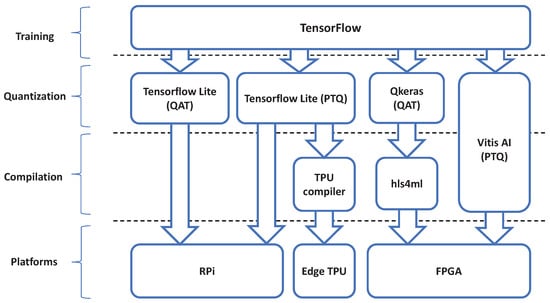
Figure 1.
Tool flows for embedding a CNN on different embedded devices. Tensorflow, the general framework for training CNNs, is at the top. Going down, the tools for converting the floating point models to fixed point models (Post-Training Quantization or Qantized Aware Training) is below this. Under that, for certain platforms, the tools for compiling the quantized models depending on the specific platform. At the bottom, the embedded platforms are displayed. Notice that Vitis AI performs both quantization and compilation.
On top is the general framework for training the models, here this is TensorFlow. TensorFlow also features an extension called Tensor Flow Lite (TFLite) [12], for inference on mobile and embedded devices [12]. Depending on the embedded device, a different tool is required to embed the model. TFLite is used, for instance, for the RPi and the Coral Dev Board, while for the FPGA either Vitis AI [10] or QKeras in combination with hls4ml [9] is used. Each of these tools support optimizations to reduce the CNN model complexity while preserving the original accuracy.
4.1. Platforms
Five types of platforms are used to evaluate embedded CNN models for ESR. One general purpose embedded platform in combination with two ASIC design based platforms is seen in Figure 2. Furthermore, two Xilinx FPGAs used to evaluate the performance and compare the technology of the previously mentioned platforms against FPGAs, is seen in Figure 3.
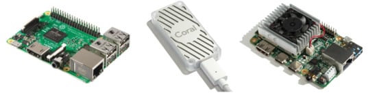
Figure 2.
General-purpose embedded platforms and TPU-based platforms: RPi 4B (left), USB Coral TPU (center) and Coral Devboard (right).
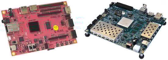
Figure 3.
The Pynq-z2 (left) and ZCU104 (right) boards are the FPGA platforms used in the analysis.
- High-end general-purpose embedded platforms
- –
- Raspberry Pi 4B: The RPi 4B+ is equipped with a quad-core 64-bit BCM 2711 SoC (ARM Cortex A72 cores) and 4 GB of RAM [34]. Previous deep learning benchmarks [35] show a significant speedup as compared to previous RPi platforms.
- TPU-based platforms
- –
- USB Coral TPU: The USB Coral is a hardware accelerator for deep neural networks written in TFLite. It was developed by Google for the fast and power efficient inference of quantized models. The first version of the USB Coral TPU was released in 2017 [36]. It has a USB 3.0 interface for communication [37]. For the evaluation of the first CNN model, the USB Coral is connected to a RPi 4B over USB.
- –
- Coral DevBoard: The Coral DevBoard is a single-board computer with a TPU SoM on the same module. The overhead caused by the USB interface that is present with the USB Coral disappears, producing a positive effect on the inference time, compared to a RPi + USB Coral combination [8]. The DevBoard has a quad-core NXP i.MX 8M SoC (ARM Cortex A53 and Cortex-M4F cores) and 1 GB of RAM [38].
- FPGAs
- –
- Zynq Z-7020 SoC: This is a low cost FPGA with a limited amount of resources [39]. It is becoming very popular, as it is the FPGA featured on the Pynq-Z2 development board (Figure 3). The low price of this board in combination with the simplicity of the Pynq framework makes this a good board for educational purposes and starters with little knowledge of FPGAs.
- –
- Zynq UltraScale+ XCZU7EV MPSoC: The second target platform, the ZCU104 board, contains a Zynq UltraScale+ XCZU7EV MPSoC. The ZCU104 is one of the two embedded boards that have pre-build reference designs for Vitis AI. The large amount of resources allow developers to place multiple DPU cores on the Programming Logic (PL). The ZCU104 features a Quad core ARM Cortex-A53 MPCore [40].
4.2. Optimizations
Before inference is possible on an embedded platform, small adaptations are required to the CNN model. These adaptations are required because of the difference in architecture between a PC and an embedded platform. Moreover, they help to improve the performance of the models when ported to embedded platforms. Examples of such modifications are quantization and model pruning, which are explained in this subsection.
4.2.1. Model Quantization
Although models are trained using floating point numbers, most embedded devices reach better performance when using fixed-point. To bridge this gap, the floating point models are quantized. Quantizing a CNN model converts the model parameters from a floating point representation to a fixed-point representation.
Post-Training Quantization
One technique to convert a floating point CNN model to fixed point is by first training the CNN model and quantizing the weights after training, hence the name Post-Training Quantization (PTQ). As the precision of the numbers changes, the accuracy of the CNN model also changes. Although the accuracy can increase, overall, most of the time the accuracy will decrease. The number of bits for the parameters in fixed point representation can also change, depending on the tool used. Hence, a 32-bit floating point CNN model can be converted to a 5-bit fixed-point representation.
Besides Keras, TFLite [12] offers a set of tools to convert and run models on embedded devices. It is used to convert trained Keras models from the ’.h5’ format to the more lightweight ’.tflite’ format, suitable for the RPi and other embedded devices. It also comes with a toolbox providing possibilities to speed up the embedded inference or to ensure high accuracy while using quantized models. In this paper, TFLite v2.5.0 is used.
Quantization Aware Training
An alternative for PTQ is Quantization Aware Training (QAT), which uses quantized parameters to train the model. The advantage of QAT over PTQ is that it has a higher accuracy, or a smaller loss in accuracy, after quantization, but it also takes longer to train the model. Furthermore, the error of the model that is used to update these parameters during training is still calculated as a floating point number.
Although TensorFlow does support QAT, it still stores the model parameters as 32-bit floating point numbers. As a result, the model needs to be quantized again using TFLite after training the model. An alternative approach to this is using QKeras for QAT [19,41]. Qkeras is a framework for QAT of TensorFlow models, specifically aimed toward compressing models for hardware accelerators while providing high accuracy, low latency, and minimal energy consumption. QKeras has the advantage over standard TensorFlow quantization in that it allows more control over the number of bits used for the parameters. TensorFlow, for example, only supports 8, 16 or 32-bit fixed point numbers, where QKeras allows controlling the exact number of bits. Despite the fact that QKeras is more flexible, it is not supported on the RPi or the Coral Dev Board. These platforms only support TFLite. Hence, QKeras is only used for hls4ml and TFLite is used on the other platforms.
Besides hls4ml, another tool also exists for embedding CNNs on FPGAs: Vitis AI, which is described in full in Section 6. Vitis AI not only supports PTQ and QAT, but also a third quantization technique called Fast Finetuning or Advanced Calibration. This technique uses the AdaQuant algorithm [42], but can only be used for Pytorch and is in development for TensorFlow 2. In this paper, only PTQ is evaluated for Vitis AI.
4.2.2. Model Pruning
In addition to quantization, pruning, also called sparsity, helps in embedding models. Pruning reduces the size of the model by setting a predefined number of weights to zero during training [18]. After training, the multiplications involving weights that are set to zero are removed from the model. Although TFLite has an API for model pruning [43], it does not have an impact on the inference time or the size of the model on the disk. Nevertheless, hls4ml removes any multiplication involving weights that are set to zero, thus saving resources on the FPGA.
Vitis AI, a free and open source tool developed by Xilinx for embedding CNNs on FPGAs using a DPU, also supports model pruning through the Vitis AI optimizer. The Vitis AI optimizer requires a commercial license, unlike the other parts of Vitis AI, which have no license cost. Because the Vitis AI optimizer does not support Tensorflow 2 and only supports TensorFlow 1.15 [44], Vitis AI is used without the optimizer in this paper. It is worth noting that for Vitis AI, pruning does not save resources as the resource consumption is independent of the model. Instead, it only improves the latency and throughput of the model.
4.3. Tool Flows
Depending on the platform used, some different tools and additional steps are required to embed CNN models.
4.3.1. Tool Flows for TPU
The fixed architecture of TPUs limits some model optimizations. For instance, to run inference on the TPU, it is necessary that the models are quantized to an 8-bit integer format. These quantized models also need to be compiled for the TPU using Google’s Edge TPU compiler [11]. In this work, v15.0 is used. This converts a ’.tflite’-model to a model compatible with the TPU and maps the unsupported operations to the CPU of the host. Figure 4 shows the tool flow used to deploy a model on a Coral device.
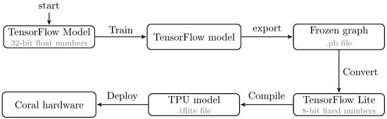
Figure 4.
Tool flow for embedding a model on the Coral Dev Board. On top is the standard training procedure, at the bottom, the specific steps to export the trained model to the board.
It is important to note that the TPU compiler currently has an important limitation in that the TPU does not support all operations, and thus some operations are executed on the CPU [45]. In the current version of the compiler, all operations after the first non supported operation are also mapped on the CPU [45]. This CPU is slower than the TPU itself, which means that the architecture of the model can have a big impact on the performance of the model on the TPU [8].
4.3.2. Tool Flows for FPGAs
- Dataflow Architectures: Several tool flows exist for embedding CNN models on FPGAs in a dataflow fashion. These approaches fully allocate all the layers of the model using the resources of the FPGA. Their advantage is that the implemented solutions operate in streaming, achieving very low latencies due to pipeline the execution of the layers of the CNN model. One popular tool is FINN [46], which generates pipelined streaming architectures for Xilinx FPGAs using Brevitas [47], a research library for QAT in Pytorch. However, it does not support TensorFlow models, which limits the portability of CNN models to other hardware accelerators such as the Coral TPU. Similarly, hls4ml is an open-source tool that, unlike FINN, does support TensorFlow. Just like FINN, it generates a streaming design in High-Levels Systhesis (HLS), with additional support for external tools such as Qkeras.The hls4ml framework [23] is one of the tool flows used for this evaluation, mainly because of its streaming approach and its compatibility with TensorFlow. It also offers the possibility to convert a Keras model to fixed-point representation through PTQ or it can be used with Qkeras for QAT. An overview of the tool flow is given in Figure 5. After setting the desired configuration and choosing the FPGA part, the fixed-point model is compiled into High Level Synthesis C++ code. This HLS code is pre-synthesized using Vivado HLS, after which it is exported to generate Register-Transfer Level (RTL) code. The exported RTL is available as an IP block in Vivado, where it can be used in a HDL design. In this paper, hls4ml v0.5.1 is used.
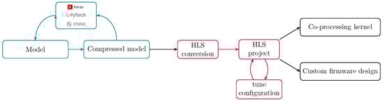 Figure 5. hls4ml tool flow as presented in [9].
 - Matrix of Processing Elements: Alternative approaches based on a matrix of processing elements, more similar to GPUs and TPUs, also exist for FPGAs. An example is Vitis AI [10] from Xilinx, which uses a general purpose DPU architecture that is placed in the PL. Vitis AI has a similar tool flow to the TPU: after training, the model is quantized and compiled. Vitis AI is fully open-source [48], except for the DPU, which is provided as an encrypted IP that can be used in Vivado or Vitis to be allocated in the design. There are several different versions of the DPU depending on the FPGA used. For embedded devices, like the ZCU102 or ZCU104, there is only one DPU available: the DPUCZDX8G [49]. This is a DPU designed for general purpose CNN applications with 8-bit quantization. There are also other versions of the DPU like the DPUCADF8H, which is designed for high throughput and is supported on the U200 and U250 Alveo cards. In Section 6, the Vitis AI tool flow is used to evaluate and compare the implementation of a CNN model on an FPGA against TPU-based platforms. In this paper, Vitis AI v1.3.2, together with DPU version 1.3 and Vitis/Vivado 2020.2, are used.
5. Embedding a 1D CNN Model for ESR: FPGAs against Embedded Platforms with TPUs
The first CNN model for ESR of our evaluation is a 1D CNN model. The proposed CNN model is designed to be small in order to fit on low cost FPGA with limited resources. This novel CNN model has one-dimensional convolutional layers and takes as input a vector of spectro-temporal features such as the ones described in Section 3.2. The FPGA-based solution implemented using hls4ml is compared against two other platforms: the coral DevBoard and the RPi 4 with/without the USB Coral TPU.
Before the FPGA solution can be compared, it first requires optimizations to reduce the resource consumption of the model on the FPGA so that the model fits on the FPGA. As these optimizations have a negative impact on the accuracy and also influence the inference time, one has to find an optimal solution that reduces the resource consumption of each type of resource on the FPGA, while not sacrificing accuracy. It is for this reason that first, the effects of the optimizations in hls4ml are evaluated to find an optimal implementation of the model before the hls4ml solution is compared against the other platforms.
5.1. Description of a CNN with 1D Spectro-Temporal Features as Input
Our proposed CNN model has the goal of being a lightweight CNN for embedded devices. The layers of this model are showed in Table 1. The input features that are all of the features presented in Section 3.2. Similarly, the datasets also presented in the same section are used to evaluate its performance.

Table 1.
Overview of our proposed 1D CNN model. It will be used as a reference when comparing to embedded solutions.
Although the proposed CNN model is designed to be lightweight in terms of the number of parameters, the CNN model is still too large for hls4ml. Moreover, this tool does not currently support dense layers with a multidimensional input. As a result, some modifications are needed. All modifications made to the CNN model for compatibility with hls4ml are marked in bold in Table 2. The first modification involves flattening the output feature map after the last convolutional layer, so that the next dense layer gets a one-dimensional input. To reduce the number of parameters, the number of filters is also reduced in each convolutional layer, together with the number of neurons in the first dense layer. For the rest of the paper, this CNN model is referred to as the CNN1D model as it takes one-dimensional inputs and outputs of 1D convolutional layers.
Table 2.
Adjustments of our proposed CNN1D model. All modifications highlighted in bold for compatibility with hls4ml.
As expected, the accuracy achieved with the CNN model outperforms, in most of the cases, the accuracy of using classical machine learning as reported in the literature (Table 3). Although other CNN models can outperform our proposed one, they have a higher complexity and a high number of parameters. Such large models present a lower throughput when executed on embedded devices, which do not make them good candidates to be embedded on small FPGAs. However, as a consequence of the modifications, the overall accuracy of the CNN1D decreases compared to the original proposed CNN model. An inevitable consequence of the modifications to the network to make the CNN1D model compatible with the entire tool flow of hls4ml.
Table 3.
Classifiers’ accuracy and standard deviation per dataset reported in the literature [6] compared to the proposed CNN model.
5.2. Steps Through hls4ml
Figure 6 summarizes the steps in the methodology, reflecting the modifications and optimizations required to port the CNN1D model to an FPGA using hls4ml. They include the comparison of the full precision model with a fixed-point version, which is used as baseline for the optimizations available in hls4ml.

Figure 6.
The steps through hls4ml to port a model.
5.2.1. Accuracy Baseline
Full Precision Baseline
The baseline performance is defined as the accuracy of the 32-bit floating point model. For the CNN1D, the model is trained five times using 5-fold cross validation. This means that each time the model is trained, a different set of training, validation and test data is used like with UrbanSound8k (Section 3.1). The main difference is that for UrbanSound8k, 10 folds are used, and here, only 5 folds are used. As a result, the model parameters are different after each training. Hence, the accuracy of the model is also different. From these five trained models, the average accuracy and standard deviation are used to obtain representative results per model and per dataset. This full precision baseline is depicted in Table 3.
hls4ml Baseline
After training the baseline floating point models, a first step is to also define a baseline in hls4ml. The process consists of converting a Keras (.h5) model to hls4ml by replacing all of the floating point parameters by their fixed-point representations. This is done because fixed-point calculations are not as expensive as floating point calculations on an FPGA, both in terms of resources, latency and energy consumption. Therefore, the use of fixed-point number representation is a logical consequence when building a design for an FPGA. It is also desirable that the hls4ml models have the same accuracy as their Keras counterparts. Because the direct conversion using PTQ shows accuracy degradation when using less than 32 bits, 32-bit fixed-point numbers are used in the hls4ml baseline.
5.2.2. Optimizations
hls4ml has a set of optimizations available to optimize the performance and resource consumption of a model [9]. To identify the contribution and effect of each optimization on the resource consumption, inference time, and accuracy, each optimization is evaluated. Based on the results of the evaluations, an optimized design is generated for comparing hls4ml against the other embedded devices. The three parameters that are evaluated are the following:
- Quantization: The number of bits used in the fixed-point representation of the model parameters and feature maps. Naturally, this has an effect on the resources consumed by the design.
- Pruning: The portion of weights in the network that are set to zero. This results in less calculations and also affects the resource consumption.
- Reusability: A reuse factor defines the number of times a multiplier is reused.
Quantization and pruning are already described in Section 4.2 and are related to the model parameters itself. The reusability, however, is an optimization related to how the model is implemented in the FPGA. The factor of reuse, as defined in hls4ml, influences the used resources and latency at deployment on the FPGA by determining the level of parallelism. For instance, a reuse factor of 1 means that each multiplier in a layer is only used once and is thus fully parallel. This also increases the resource consumption since the multiplier is implemented multiple times to ensure the desired parallelism. On the other hand, using a maximal reuse factor results in a single multiplier, saving resources but increasing the latency, as it prevents parallel computations on the layer level.
5.3. Evaluation of the hls4ml Baseline
The performance of the 32-bit fixed-point baseline is used as reference for a later comparison with the optimized solutions. Since the goal is to embed the model on the FPGA for real-time sound recognition, parameters such as the resource consumption and the execution time or latency are crucial.
5.3.1. Latency
The latency is the time it takes for the model to generate an output, after receiving an input vector, hence, it is the same as the inference time. On FPGAs, latency can be expressed as a number of clock cycles or as a duration in seconds. The number of clock cycles can easily be calculated after Vivado HLS pre-synthesis. Together with the estimated clock frequency, it provides an estimation of the latency in seconds.
Another useful parameter is the II. This is the time it takes between two consecutive calculations of an output vector. The II can differ from the latency when the design is pipelined. In this way, the different layers can compute their feature maps in parallel, allowing multiple operations of different input vectors at the same time in the functional block. hls4ml creates a streaming design and automatically performs high-level pipelining. This brings as an advantage, that the throughput can be higher than without pipelining.
After pre-synthesis in Vivado HLS, the tool gives the expected latency and initiation interval of the design, together with a first rough estimation of the clock frequency. When synthesized in Vivado subsequently, a new clock frequency is estimated. The estimation after synthesis is a more realistic one than the one after pre-synthesis. Table 4 shows that the pre-synthesis clock period is a rather optimistic underestimation, since the synthesis clock period is more than double its value. When expressed in seconds, the latency and II after synthesis are, respectively, 16.4 ms and 9.9 ms for the CNN1D baseline solution. It is interesting to remark that, for this CNN1D model, the value of II corresponds to the most time demanding layer of the model, which corresponds to the first dense layer.
Table 4.
Timing summary baseline CNN1D as reported in Vivado HLS and after the synthesis in Vivado.
5.3.2. Resource Consumption
The resource consumption provides information regarding the suitability of the model to be allocated on the FPGA. In order to minimize the resource consumption, the highest possible reuse factor of the multipliers in each layer is applied. Where the latency is underestimated, the resource consumption is highly overestimated. Figure 7 exemplifies how inaccurate the pre-synthesis estimations of Vivado HLS are when compared to the synthesis estimations, with the exception of the DSP blocks consumption. It should be noted that the pre-synthesis gives no LUTRAM estimation, but uses BRAM instead. Nonetheless, the hls4ml baseline CNN1D model does not fit on the Zynq Z-7020 due to its large resource demand.
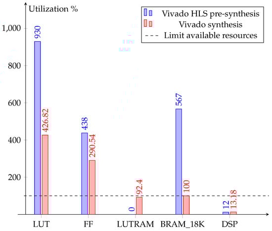
Figure 7.
Resource estimation comparison between pre-synthesis and synthesis for the baseline CNN1D model on the Zynq Z-7020.
5.4. Model Compression
The oversized hls4ml baseline version of the CNN1D model is certainly not acceptable for small FPGAs. Moreover, this version does not take advantage of the full potential of hls4ml. The different optimizations available in hls4ml are used to reduce the model size, at the cost of certain accuracy drop.
5.4.1. Quantization Aware Training with Qkeras
Model compression is necessary to reduce the model size, thus saving resources on the FPGA. The first compression step has the goal of quantizing the model parameters to a lower number of bits. Because PTQ can affect the accuracy negatively due to rounding or wrap around errors when using a low number of bits, the models are QAT with Qkeras. The desirable model has the least amount of bits possible, while keeping the accuracy close to the baseline accuracy. Although it is possible to fine tune the number of bits in each layer individually, for this paper, all layers use the same number of bits as this helps to draw more general conclusions.
Figure 8 shows the effect on the accuracy of QAT with different number of bits in Qkeras for the CNN1D model. For different number of bits of the CNN1D model, it is clear that the accuracy stays at the baseline level until quantization to one bit (a binary neural network). The choice is made to use 3-bit quantized models for deployment onto the FPGA, which still ensures good accuracy while compressing the models as much as possible.
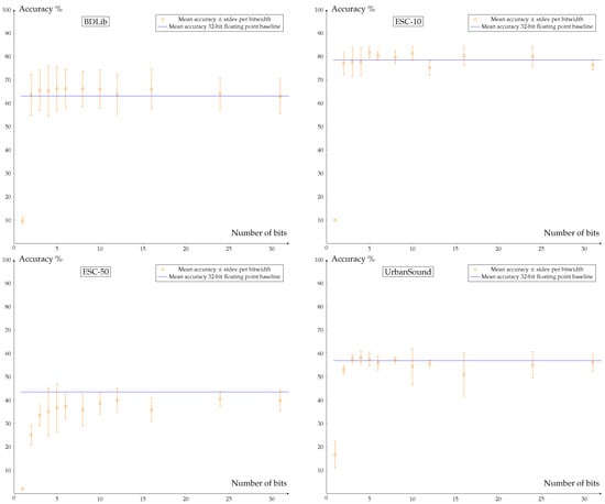
Figure 8.
Accuracy of models after QAT depending on the number of bits for the model parameters after quantizing the model. The blue line represents the accuracy of the floating point model. A clear degradation in accuracy can be observed when using one bit, while using three or more bits only results in a minor loss of accuracy.
5.4.2. Training with Sparsity
A second method that is used to compress the models is training with sparsity. For the experiments in this paper, a pruning schedule with constant sparsity is used. This implies that during the whole training, the number of weights that are set to zero is constant. More complex pruning schedules are possible, but they are not used here. To find the ideal sparsity to be used further in the next steps, experiments are performed to see the effect of different levels of sparsity on the accuracy. The models are trained using QAT with 3-bit quantization. Figure 9 shows that the accuracy of the CNN1D models starts to drop at a sparsity level of 80%.
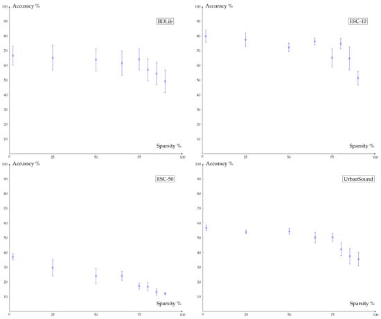
Figure 9.
Accuracy of the (trained) models for different levels of sparsity. Only a small degradation in accuracy can be observed up to 75% sparsity. Above 75% sparsity, the accuracy drops significantly.
Based on the results of these experiments, it is decided to use 3-bit quantized and 75% sparse models for conversion of the CNN1D to hls4ml. Using this method, the accuracy is kept close to the baseline level, while the future resource consumption on FPGA becomes minimal. Figure 10 shows the evolution of the accuracy for the CNN1D models after each modification step, together with the accuracy after the final model optimizations. The decisions concerning quantization and sparsity level are based on the results from experiments with the selected dataset.
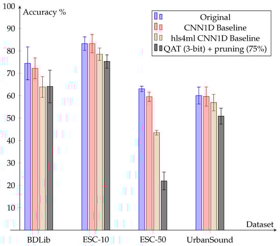
Figure 10.
Accuracy evolution after modifications and optimizations for the CNN1D model.
5.4.3. Optimized Version for Resources
A maximal reuse factor is retained for all layers as previously performed for the baseline. The results for CNN1D, concerning resource utilization of different quantization and sparsity levels are compared with the baseline in Table 5. It shows that the 8-bit model already fits. As expected, the 3-bit models use the least resources. For the 3-bit models: the BRAM utilization is reduced to 33%, the DSP utilization is only 3%, the LUT utilization is 18%, the FF utilization is 11% and finally the LUTRAM is still 79% of the baseline usage. However, the sparsity of the models does not seem to have a significant effect. The lack of the effect of sparsity on the resource utilization can be explained by the fact that the reuse factor is maximal and the amount of used DSPs is also very small. The consequence of this is that no DSPs can be dropped for the multiplications with zero, as intended when making use of sparse models.
Table 5.
Resource consumption (% of available resources of the Zynq Z-7020 FPGA) of the CNN1D designs with maximal reuse factor, % sp. stands for percentage of sparsity.
After finding an optimal resource solution for the 3-bit models, the latency of the CNN1D model is observed to be approximately the same as the baseline latency. This is already expected, since no modifications are made to improve the latency.
5.4.4. Optimized Version for Resources and Latency
In the previous designs, a maximal reuse factor is used to limit the resource consumption. Since these kinds of solutions fail to exploit the parallel nature of FPGAs and CNNs fully, an alternative solution is to optimize the latency. A new design can be allocated in a resource constrained Zynq Z-7020 FPGA while achieving the lowest possible latency. Therefore, it is necessary to adjust the reuse factors of the hls4ml configuration in a right way for each layer. The timing summaries of the baseline given in Table 6 show that specific layers, e.g., the convolutional layers and Dense_1, correspond to the majority of the introduced latency. The latency of these bottleneck layers can be reduced by using a lower reuse factor. As a result, the II benefits maximally from the inter-layer parallelism. This has also a positive effect on the latency.
Table 6.
Comparison of the latency per layer and II achieved with the hls4ml baseline model and the optimized version for resources and latency (CNN1D). All values are in clock cycles.
The latency of each layer of the optimized version of the model can be found in Table 6. The convolutional layers are now the ones that induce most of the latency. With around 6000 clock cycles, the latency of all these layers is approximately the same, which has been set as a goal to optimize the latency and II. Because of this, it is even clearer than before that the inter-layer parallelism is well exploited since the total latency (9432 clock cycles) is smaller than the sum of all latencies (23,153 clock cycles). Since the clock period stays the same, the latency of this solution is 96.8 times lower than the one from the baseline, and the new II is 79 times lower than the baseline II. When combining the results with a clock period of 18 ns, the new latency is 0.17 ms (compared to 16.4 ms for the baseline) and the new II is 0.13 ms (compared to 9.9 ms for the baseline).
Table 7 shows a comparison of the resource utilization of the solution with optimizations for latency and the solution with optimizations for resource consumption. Notice how the LUT utilization limits further optimizations towards lower latency, because the available LUTs are almost fully used. Compared to the low-resource design, the utilization of LUTs and FFs increases by 22.1 % and 39.5 %, respectively. The other resources have similar or slightly lower utilization than in the resource strategy design. However, the increase in resources does not directly lead to a decrease in latency. Smart tuning the hls4ml configuration by choosing the right reuse factors, combined with model compression during quantization, allows low resource consumption with low latency to fit a model to the constraints of an FPGA.
Table 7.
Resource consumption (% of available resources of the Zynq Z-7020 FPGA) comparison of the solutions optimized for resources and latency of the CNN1D.
Figure 11 summarizes the resource consumption on the Zynq Z-7020 of all evaluated solutions designed for CNN1D. It turns out that reducing the number of bits during quantization is the most effective compression technique and saves the most amount of resources. While decreasing the reuse factors has a big effect on the latency, the effect on the resource consumption is rather limited.
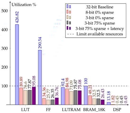
Figure 11.
Vivado synthesis: Resource usage (% of available resources of the Zynq Z-7020 FPGA) for different model configurations, with maximal reuse factor for each layer and the latency-optimized solution with optimized reuse factors.
5.5. Evaluating Embedded Platforms with TPUs
As previously mentioned, one of the goals of this paper is to compare FPGA-based solutions such as hls4ml, against other embedded platforms. The results for CNN1D on each of the embedded devices of Section 4.1 can be found in Table 8, Table 9, Table 10 and Table 11. The tables include inference times for both a PTQ and QAT model on the RPi as well as a RPi combined with a USB TPU, the Coral dev board and the hls4ml solution. Note that for the models on the TPU, only PTQ models are used since support for QAT models is still under development for the TPU compiler.
Table 8.
CNN1D: Zynq Z-7020 vs. other embedded devices for the BDLib dataset.
Table 9.
CNN1D: Zynq Z-7020 vs. other embedded devices for the ESC-10 dataset.
Table 10.
CNN1D: Zynq Z-7020 vs. other embedded devices for the ESC-50 dataset.
Table 11.
CNN1D: Zynq Z-7020 vs. other embedded devices for the UrbanSound dataset.
A few conclusions can be made based on the results in the tables:
- The quantized models generally have a lower inference time than the non-quantized models on the same device. This is the expected result since these quantized models are smaller and computationally less intensive than their non-quantized counterparts.
- The PTQ models can show a clear decrease in accuracy. For the quantized models that use QAT, the accuracy is always the same or even better than that of the floating point models.
- The CNN1D PTQ models are faster than the QAT models. This is because, for the QAT, 1D convolutional layers are not supported, so they are replaced by an equivalent two-dimensional representation with exactly the same effect. The inference time of the models increases when using this method, which indicates a bigger overhead when using 2D convolutional layers.
- The CNN1D models are slower when using the TPU as an accelerator than without using the TPU. This can be explained by the fact that not all used operations are supported for execution on the TPU. When the compiler encounters an unsupported operation, it maps this operation and the subsequent operations back to the CPU of the host. As a consequence, only a few layers are accelerated on the TPU. The rest of the layers have the latency inherent to the CPU of the host. In addition, the communication overhead between CPU and TPU results in a slower inference time than without making use of the TPU.
5.6. Conclusions of the Technology Comparison
To place the performance on the FPGAs into context, the Zynq Z-7020 with CNN1D is compared with the RPi 4B and the Coral DevBoard + TPU in Table 8, Table 9, Table 10 and Table 11 for all datasets. The solution generated using hls4ml for the Zynq Z-7020 FPGA is faster than any solution on other devices (PTQ 8-bit model on a RPi 4B), while maintaining a high accuracy. The best performing model on embedded devices that is still on the level of the full precision accuracy (QAT 8-bit on RPi 4B) is outperformed by the FPGA by 40% in inference time. The throughput is even doubled, taking advantage of the streaming model of the FPGA design.
When compared to the best solution that uses a dedicated TPU (PTQ 8-bit on the Coral DevBoard + TPU), the FPGA achieves both better accuracy and a speedup of 75%. However, this should be placed into perspective because the capabilities of the TPU could not be fully exploited due to unsupported operations.
6. Embedding a 2D CNN Model for ESR: Comparing DPUs and TPUs
Our CNN1D cannot fully exploit the TPU capabilities, which could lead to biased conclusions regarding the performance of FPGAs when compared to TPUs. Moreover, many CNN-based models do not use features as input, but rather images or, for audio signals, spectrograms. To compare the technologies when looking for the most performing solution for ESR applications, another CNN-based model is adapted for TPUs is evaluated. This time the Xilinx DPU is also included in the evaluation in order to compare similar deep learning approaches. This comparison enlarges the number of tool flows involved since the Xilinx DPUs are implemented using Vitis AI, another tool from Xilinx to embed CNNs on FPGAs. Although the previous datasets are perfectly valid for the evaluation of CNNs, most of them are not large enough to satisfy the recommendable minimums to evaluate Vitis AI solutions. As a solution, UrbanSound8K [31], an extended version or the UrbanSound dataset, is the dataset used for this comparison.
6.1. A Spectrogram-Based CNN2D Model
The model proposed in [27] is selected for this comparison due to its relatively small size and relative high accuracy. To be fully supported by hls4ml and Vitis AI, the model needs to be adjusted. The modifications needed include:
- The size of the pooling layers needs to be changed from to because hls4ml only supports square pooling layers.
- A max pooling layer is added between the third Relu layer and the flatten layer. This modification reduces the number of connections in the first Relu layer after the flatten layer, which is the layer containing the most amount of weights in the model. By adding the max pooling layer, the number of weights in the Relu layer is reduced from 307,264 to 27,712, which results in a reduction of the total amount of weights from 395,034 to 115,482. Moreover, the reduction of the amount of weights helps save resources when using the hls4ml approach to embed the CNN on the FPGA.
An overview of the layers and the number of parameters in each layer of the model can be found in Table 12.
Table 12.
Overview of the layers in the modified model (CNN2D).
Besides the changes to the model itself, the training strategy also demands minor modifications. To begin with, no data augmentation is used during training. The first three seconds from each audio file are taken for generating the spectrograms like the training data in [32], instead of using a random position as performed in the original work [27]. Audio files with less than three seconds of audio are repeated to generate three seconds of audio. These three second audio fragments are converted to mel spectrograms using the librosa’s melspectrogram function [50]. The hop length and FFT window length are both 1024 samples, and the number of mel bands is equal to 128. This results in grayscale spectrograms with a resolution of . Each spectrogram is normalized on the range of zero to one.
Then, instead of using mini-batch stochastic gradient descent and 50 epochs, the Adam optimizer is used with a learning rate of 0.001 for 100 epochs with a batch size of 30. After each epoch, the model is evaluated on one of the nine folds used for training and the model with the highest evaluation score is saved. To ensure that the validation fold and the test fold are never the same, the validation fold is set to the fold before the test fold. This means that if fold 10 is the test fold, folds 1 through 8 are used for training and fold 9 for validation. For test fold 1, fold 10 is used for validation and folds 2 through 9 for training. Nonetheless, these changes decrease the average test accuracy for all 10 folds from an original 79% to 63.88%.
6.2. FPGAs
The modified CNN model, referred as CNN2D from here on, is implemented on FPGAs using two different tool flows: hls4ml and Vitis AI.
6.2.1. hls4ml
To embed the model using hls4ml, a similar approach is taken as for the CNN1D model to find the optimal configuration. The intermediate results from these experiments are not discussed in depth here as they show a similar pattern to the ones of the CNN1D. Instead, an overview of the configuration is given.
To get optimal accuracy using a low number of bits, the models are trained using QAT without model pruning. Because for a very low bit width (3-bit) QAT shows a reduction of the accuracy compared to the baseline and because Vitis AI uses 8-bit quantization, 8-bit quantization is also used for the hls4ml model. The reuse factors are tuned in such a way that the latency is optimized, while the resource consumption stays within the boundaries of the ZCU104. It should be noted that there are not sufficient LUTs available, as seen in Table 13 because a large amount of LUTRAM is used.
Table 13.
Resource consumption (% of available resources) of CNN2D on the ZCU104 with hls4ml.
6.2.2. Vitis AI
As mentioned before, the Vitis AI tool flow is very similar to the tool flow of the TPU. However, instead of using a TPU with a fixed architecture to infer models, a configurable DPU is used. Xilinx provides a docker container with all necessary libraries and tools installed to quantize and compile models for the DPU. Two of these tools are the Vitis AI quantizer and Vitis AI compiler. First, the Vitis AI quantizer quantizes a trained model. This process requires a set of unlabeled input data to optimize the quantized weights [49]. After quantization, the quantized model can be tested inside the docker container before deployment on the FPGA. The second tool, the vitis AI compiler, compiles the quantized model to a set of proprietary DPU assembly instructions based on the configuration of the DPU IP. Depending on the version of the framework used, these tools come in the form of python functions or shell scripts.
This configuration controls the active layers and the performance of the DPU. When a model does not use specific layers, the corresponding operations can be disabled in the DPU to save resources without impacting the performance of the model. Examples of such layers are average pooling, leakyRelu and softmax, which can be disabled. For instance, because the CNN2D model does not use average pooling or leakyRelu, both of the operations are disabled, thus saving between 1854 and 4096 LUTs depending on the size of the DPU architecture [51]. Similarly, the softmax layer is also disabled in the design because the softmax function is only used at the end of the model. To determine the predicted class on the hard-core ARM processor of the Zynq MPSoC, the label with the highest score has to be found, and the softmax does not change which label this is, only the value of the score. However, disabling the softmax layer saves 9580 LUTs, 8019 FF, 4 BRAM and 14 DSPs. The option to enable the softmax function differs from other layers as it not only changes the internal structure of the IP, but also the connection interface of the IP by adding an extra interrupt pin and an extra AXI port. Unlike the other options, the resource consumption of the softmax function is not influenced by the DPU architecture or the number of DPU cores.
A second category of parameters address resource savings at the cost of increasing the latency. The most important one is the size of the systolic array, also called the DPU architecture. For instance, this parameter is referred to as B512 or B4096 for the smallest and the largest DPU architecture, respectively. The number 512 or 4096 stands for the peak Ops, which corresponds to the number of operations per clock cycle. The size of the DPU architecture has a direct impact on the resource consumption of other parameters such as the average pooling described previously. Nonetheless, four options of Vitis AI are changed between configurations.
- Channel augmentation: Channel augmentation improves the efficiency of the DPU when the number of input channels is less than the channel parallelism of the DPU architecture. This is most common in the first layers of a CNN, as the number of feature maps generally increases for later layers in a CNN.
- Depthwise convolution: Depthwise convolution or depthwise separable convolution changes the way convolutions are performed on the DPU by splitting the standard convolution into two convolutions: one convolution over the channels (depthwise) followed by a second convolution with a 1 × 1 filter (pointwise).
- RAM usage: The DPU uses BRAM as a buffer to store intermediate features, weights and biases. The BRAM consumption is controlled through this parameter, enabling higher or lower latency of the DPU through the consumption of BRAM.
- DSP Usage: The last option is not a straight forward reduction of resources, but rather a trade-off between types of resources. The DSP usage gives the option to replace DSPs by LUTs. In high DSP usage mode, the DPU uses DSPs for both accumulations and multiplications. In low DSP usage mode, the accumulations are performed using LUTs instead of DSPs.
Changing the configuration of the DPU influences the model execution on the DPU, for this reason, a json file is generated by Vivado or Vitis. This json file describes the DPU architecture used and has to be provided to the Vitis AI compiler when compiling the model. When the DPU does not support a layer from the model, Vitis AI can still compile the model. In this case, the model is split into several parts called subgraphs. When the model is loaded using Vitis AI runtime libraries, each subgraph indicates if execution on the DPU is allowed or not. Subgraphs that cannot be executed on the DPU are executed on the CPU instead. This results in a significant impact on the performance, as the CPU is slower than the DPU. The DPU has to be reprogrammed with the next subgraph and the data has to be transferred between the DPU and the CPU after execution of each subgraph on the DPU. Furthermore, the application code has to be adapted to execute the inference in several parts. Training and quantization of the model are not influenced by the DPU configuration and should not be repeated when the DPU configuration changes. This also means that the accuracy is not affected as it only depends on the accuracy after training and quantization. It is worth noting that the quantization used in Vitis AI is not compatible with the quantization used in the hls4ml flow. For this reason, both quantized models have a different accuracy.
Four different configurations of the DPU are used, one focusing on latency, one focusing on resource consumption, and two intermediate configurations focusing on a trade-off between resources and latency:
- Configuration 1: The first configuration focus on latency by using the largest systolic array in combination with high RAM and DSP usage and enabling both channel augmentation and depth-wise convolutions.
- Configuration 2: The second configuration also focus on latency by using the largest systolic array, but resources are saved by disabling the other options.
- Configuration 3: The third configuration is the opposite of the second configuration: it consists of the smallest systolic array to save resources and instead all other options are enabled to improve the latency like the first configuration.
- Configuration 4: The last configuration focus on resource consumption by using the smallest systolic array and disabling the other options.
The latest Xilinx Ultrascale+ FPGAs include a new type of memory blocks, UltraRAM (URAM), which largely increases the on-chip memory. The DPU can benefit from the use of this type of on-chip memory by using URAM used instead of BRAM.Since the ZCU104 includes a Zynq Ultrascale+ MPSoC FPGA, URAMs resources can be exploited. For instance, the configuration of the DPU in the Target Reference Design (TRD) of the ZCU104 consumes more BRAM than available on the board [48]. However, by enabling URAM, two DPU cores can be placed on the board, both having the largest DPU architecture. Having two DPU cores also allows either running two models at the same time or processing multiple inputs for one model in parallel.
An overview of the configurations under test can be found in Table 14. DPU version 1.3 and Vitis AI v1.3.2 are used together with Vitis 2020.2. Average pooling, element-wise multiply and leaky Relu are not used by the model and are disabled in all configurations. Each configuration uses only one DPU core, and no URAM is used. If two DPU cores are used, not all configurations fit on the board without using URAM. The DPU also needs two clock signals, one twice the frequency of the other. Here, the two clocks are set at 300 MHz and 600 MHz.
Table 14.
The four different configurations of the DPU together with the resource consumption of the configurations.
6.3. Conclusions of the Technology Comparison
The comparison of the test accuracy for each fold can be found in Table 15. Notice that all tool flows have the same average accuracy despite the fact that there is a large difference in accuracy for some folds between the tool flows. Nonetheless, there is no clear winner in terms of accuracy. During quantization, the accuracy can increase slightly due to the change in precision of the model parameters.
Table 15.
Accuracy (in %) for each fold and average accuracy across all 10 folds of the UrbanSound8k dataset for the different tool flows with the CNN2D model after quantization.
Figure 12 shows a quite different story. Firstly, the inference times are higher than the ones obtained for the CNN1D model due to the complexity that the CNN2D model presents. Whereas the optimized solution from hls4ml perform below milliseconds for CNN1D, the inference time grows to almost 3 ms for the CNN2D model. However, this is still far below the 3 s of recording time that is used to generate the spectrograms and still allows the system to operate in real time. Thanks to fully supporting all operations in the CNN2D model, the TPU outperforms the optimized hls4ml solution by a factor of two. Secondly, Xilinx DPUs present the better trade-offs in terms of inference time. The most resource-demanding configurations present a significantly lower inference time. In the best case, Xilinx DPUs are almost twice as fast as the TPU on the Coral Dev Board. The resource cost is demonstrated to be directly related to the inference time. As a result, the less-demanding DPU configuration offers a similar performance to the optimized hls4ml solution.
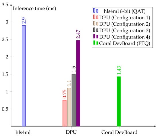
Figure 12.
Inference time (in ms) of hls4ml, different configurations of the DPU and the Coral DevBoard with the TPU.
7. Discussion and Generalization
A view of the tool flows shows that each one has its own limitations. As depicted in Table 16, the tools do not support all types of layers or models. For the TPU, the supported layers also depend on the quantization strategy, as there is a difference between supported layers for PTQ and QAT. For some layers, QAT is not yet supported and additionally, since QAT models on the TPU are still in development, it is possible that some models work perfectly fine with PTQ, but not after QAT.
Table 16.
Summary of supported layers/operations across the tool flows.
7.1. Lessons Learned with hls4ml
Based on the experiments porting CNN1D to embedded platforms, the FPGA solution with optimizations outperforms all other embedded solutions. Since the Zynq Z-7020 is a rather constrained FPGA, this makes it very suitable to be deployed for real-time urban sound recognition on the edge. Although one might think that this makes the CNN1D superior for deployment on embedded devices, the remark should be made that the time for the feature extraction is not included in these results. CNN1D uses multiple input audio features that would likely result in slower feature extraction that could possibly nullify the inference latency difference [6]. Moreover, the FPGA solution generated with hls4ml performs better than the TPU solution because some operations are not fully supported on the TPU. Nonetheless, this is one of the added values of hls4ml. Whereas popular layers are fully supported by most of the tools in Table 16, notice that 1D layers are only supported by hls4ml. Since hls4ml is an open-source tool, which is under continuous development and extension from the community, hls4ml offers support for less adopted layers, offering an interesting and competitive solution to porting custom CNN models on FPGAs.
From the experience, the major drawback of hls4ml is, perhaps, the model size. Large models lead to unacceptable resource consumption, or in some cases, the tool cannot handle the model size and crashes. Since the hls4ml tool flow limits the size of the models, concessions have to be made in terms of accuracy. Despite the fact that the models are compressed while keeping the accuracy as high as possible, there is still an inevitable loss.
7.2. Lessons Learned with DPUs and TPUs
Xilinx Vitis AI has shown very interesting results for the CNN2D model. Although DPUs present the same approach as TPUs and similar deep learning-based accelerators, they have been seen to offer competitive results while offering a certain level of flexibility. Of course, such a level of flexibility is rather limited when compared to hls4ml. While hls4ml can grow in layer and model support, the DPU is a relatively fixed and closed architecture which can only grow through modifications at the internal architecture level. Nevertheless, where hls4ml fails in support for large models, DPUs outperform equivalent TPUs. The supported modes of DPUs enable them to adjust their resource consumption to the desirable performance level. As a result, DPUs are adaptable solutions to embed complex models on FPGAs.
7.3. General Lessons
The tool flows to embed CNN models on FPGAs have been shown to be mature enough to provide competitive alternatives to other hardware accelerators such as TPUs. Following one of the main characteristics of FPGAs, the flexibility shown by hls4ml and Xilinx Vitis AI demonstrates that there is no unique solution when using FPGA, but rather the opposite. Low complex, small or customized CNN models can benefit from hls4ml. Thanks to the streaming architecture it generates, the model can be optimized to pipeline solutions with low II, something that is not possible on the other embedded platforms. Larger models, on the other hand, can achieve high throughputs when ported to Xilinx DPUs. Despite their limited supported modes, DPUs can fully exploit available resources, making FPGAs outperform TPUs.
8. Conclusions
The journey of developing CNN-based sound classifiers for embedded platforms provides us an excuse to evaluate different tool flows and technologies. Relatively small and low complex CNN models have shown that they can be exploited by using streaming architectures like the ones generated with hls4ml, an open-source tool flow to port CNNs on FPGAs. Although the obtained solutions outperform general-purpose embedded devices such as RPi platforms, dedicated hardware accelerators, such as TPUs, promise higher performance when embedding CNN models. However, the experiments have demonstrated that, although Xilinx DPUs use an architecture approach similar to TPUs, they can exploit FPGA resources toward outperforming TPUs. As a result, tool flows to embed CNN models on FPGAs have been demonstrated to be flexible enough to support and to produce high-performance solutions.
Author Contributions
Conceptualization, B.d.S. and A.T.; methodology, J.V., N.W. and B.d.S.; software, J.V., N.W. and M.L.; validation, J.V. and N.W.; investigation, J.V., N.W. and B.d.S.; data curation, J.V. and N.W.; writing—original draft preparation, J.V., N.W. and B.d.S.; writing—review and editing, J.V., N.W. and B.d.S.; visualization, J.V., N.W. and B.d.S.; supervision, B.d.S., M.Y.C. and A.T.; project administration, B.d.S. and A.T.; funding acquisition, A.T. All authors have read and agreed to the published version of the manuscript.
Funding
This work is part of the COllective Research NETworking (CORNET) project “AITIA: Embedded AI Techniques for Industrial Applications” [52]. The Belgian partners are funded by VLAIO under grant number HBC.2018.0491, while the German partners are funded by the BMWi (Federal Ministry for Economic Affairs and Energy) under IGF-Project Number 249 EBG. The authors would like to thank Xilinx for the provided software and hardware under the Xilinx University Program donation.
Data Availability Statement
Models and code are available in: https://gitlab.com/etrovub/embedded-systems/publications/embedded-esr.
Conflicts of Interest
The authors declare no conflict of interest.
Abbreviations
The following abbreviations are used in this manuscript:
| Advanced eXtensible Interface | AXI |
| Application Programming Interface | API |
| Application-Specific Integrated Circuit | ASIC |
| Artificial Intelligence | AI |
| Block RAM | BRAM_18k |
| Central Processing Unit | CPU |
| Convolutional Neural Network | CNN |
| Deep Neural Network | DNN |
| Deep Processing Unit | DPU |
| Digital Signal Processing slice | DSP |
| Environmental Sound Classification | ESC |
| Environmental Sound Recognition | ESR |
| Fast Fourier Transform | FFT |
| Field-Programmable Gate Array | FPGA |
| Flip FLop | FF |
| Graphical Processing Unit | GPU |
| Hardware Description Language | HDL |
| High-Levels Synthesis | HLS |
| Initiation Interval | II |
| Intellectual Property | IP |
| Internet of Things | IoT |
| k-Nearest Neighbor | k-NN |
| Lookup Table | LUT |
| Lookup Tables as RAM | LUTRAM |
| Post-Training Quantization | PTQ |
| Programming Logic | PL |
| Quantization Aware Training | QAT |
| Random-Access Memory | RAM |
| Raspberry Pi | RPi |
| Rectified Linear Unit | ReLU |
| Register-Transfer Level | RTL |
| Support Vector Machine | SVM |
| System On Chip | SoC |
| System On Module | SoM |
| Target Reference Design | TRD |
| TensorFlow Lite | TFLite |
| Tensor Processing Unit | TPU |
| UltraRAM | URAM |
| Universal Serial Bus | USB |
References
- Adamson, A. Paris Testing Noise Radar System That Can Identify Furthermore, Ticket Loud Cars. 2019. Available online: https://www.techtimes.com/articles/245203/20190902/paris-testing-noise-radar-system-that-can-identify-and-ticket-loud-cars.htm (accessed on 7 September 2021).
- Ozkan, Y.; Barkana, B.D. Forensic Audio Analysis and Event Recognition for Smart Surveillance Systems. In Proceedings of the 2019 IEEE International Symposium on Technologies for Homeland Security (HST), Woburn, MA, USA, 5–6 November 2019; pp. 1–6. [Google Scholar] [CrossRef]
- Tsalera, E.; Papadakis, A.; Samarakou, M. Monitoring, profiling and classification of urban environmental noise using sound characteristics and the KNN algorithm. Energy Rep. 2020, 6, 223–230. [Google Scholar] [CrossRef]
- López, J.M.; Alonso, J.; Asensio, C.; Pavón, I.; Gascó, L.; de Arcas, G. A Digital Signal Processor Based Acoustic Sensor for Outdoor Noise Monitoring in Smart Cities. Sensors 2020, 20, 605. [Google Scholar] [CrossRef] [PubMed] [Green Version]
- Pak, J.w.; Kim, M.k. Convolutional neural network approach for aircraft noise detection. In Proceedings of the 2019 International Conference on Artificial Intelligence in Information and Communication (ICAIIC), Okinawa, Japan, 11–13 February 2019; pp. 430–434. [Google Scholar]
- da Silva, B.; Happi, A.W.; Braeken, A.; Touhafi, A. Evaluation of Classical Machine Learning Techniques towards Urban Sound Recognition on Embedded Systems. Appl. Sci. 2019, 9, 3885. [Google Scholar] [CrossRef] [Green Version]
- Piczak, K.J. Environmental sound classification with convolutional neural networks. In Proceedings of the 2015 IEEE 25th international workshop on machine learning for signal processing (MLSP), IEEE Computer Society, Boston, MA, USA, 17–20 September 2015; Volume 2015-November. [Google Scholar] [CrossRef]
- Rancaño, X.; Molanes, R.F.; González-Val, C.; Rodríguez-Andina, J.J.; Fariña, J. Performance Evaluation of State-of-the-Art Edge Computing Devices for DNN Inference. In Proceedings of the IECON 2020 The 46th Annual Conference of the IEEE Industrial Electronics Society, Singapore, 18–21 October 2020; pp. 2286–2291. [Google Scholar] [CrossRef]
- Duarte, J.; Han, S.; Harris, P.; Jindariani, S.; Kreinar, E.; Kreis, B.; Ngadiuba, J.; Pierini, M.; Rivera, R.; Tran, N.; et al. Fast inference of deep neural networks in FPGAs for particle physics. J. Instrum. 2018, 13, P07027. [Google Scholar] [CrossRef]
- Xilinx. Xilinx Vitis AI. 2021. Available online: https://www.xilinx.com/products/design-tools/vitis/vitis-ai.html (accessed on 25 June 2021).
- LLC., G. Edge TPU Compiler. 2020. Available online: https://coral.ai/docs/edgetpu/compiler/#system-requirements (accessed on 26 May 2021).
- LLC., G. TensorFlow Lite. 2021. Available online: https://www.tensorflow.org/lite/guide (accessed on 3 June 2021).
- Piczak, K.J. ESC: Dataset for Environmental Sound Classification. In Proceedings of the 23rd ACM International Conference on Multimedia; Association for Computing Machinery: New York, NY, USA, 2015. MM ’15. pp. 1015–1018. [Google Scholar] [CrossRef]
- Shah, S.K.; Tariq, Z.; Lee, Y. IoT based Urban Noise Monitoring in Deep Learning using Historical Reports. In Proceedings of the 2019 IEEE International Conference on Big Data (Big Data), Los Angeles, CA, USA, 9–12 December 2019; pp. 4179–4184. [Google Scholar] [CrossRef]
- Nordby, J. Environmental Sound Classification on Microcontrollers Using Convolutional Neural Networks. Master’s Thesis, Norwegian University of Life Sciences, Oslo, Norway, 2019. [Google Scholar]
- Turchet, L.; Fazekas, G.; Lagrange, M.; Ghadikolaei, H.S.; Fischione, C. The Internet of Audio Things: State of the Art, Vision, and Challenges. IEEE Internet Things J. 2020, 7, 10233–10249. [Google Scholar] [CrossRef]
- Faraone, J.; Gambardella, G.; Boland, D.; Fraser, N.; Blott, M.; Leong, P.H. Customizing low-precision deep neural networks for FPGAs. In Proceedings of the 2018 28th International Conference on Field Programmable Logic and Applications (FPL), Dublin, Ireland, 27–31 August 2018; pp. 97–973. [Google Scholar]
- Zhu, M.; Gupta, S. To prune, or not to prune: Exploring the efficacy of pruning for model compression. arXiv 2017, arXiv:1710.01878. [Google Scholar]
- Coelho, C.N.; Kuusela, A.; Li, S.; Zhuang, H.; Ngadiuba, J.; Aarrestad, T.K.; Loncar, V.; Pierini, M.; Pol, A.A.; Summers, S. Automatic heterogeneous quantization of deep neural networks for low-latency inference on the edge for particle detectors. Nat. Mach. Intell. 2021, 3, 675–686. [Google Scholar] [CrossRef]
- Abadi, M.; Agarwal, A.; Barham, P.; Brevdo, E.; Chen, Z.; Citro, C.; Corrado, G.S.; Davis, A.; Dean, J.; Devin, M.; et al. TensorFlow: Large-Scale Machine LEARNING on Heterogeneous Systems. 2015. Available online: https://www.tensorflow.org (accessed on 20 October 2021).
- Venieris, S.I.; Kouris, A.; Bouganis, C.S. Toolflows for mapping convolutional neural networks on FPGAs: A survey and future directions. arXiv 2018, arXiv:1803.05900. [Google Scholar] [CrossRef] [Green Version]
- Fahim, F.; Hawks, B.; Herwig, C.; Hirschauer, J.; Jindariani, S.; Tran, N.; Carloni, L.P.; Di Guglielmo, G.; Harris, P.; Krupa, J.; et al. hls4ml: An Open-Source Codesign Workflow to Empower Scientific Low-Power Machine Learning Devices. arXiv 2021, arXiv:2103.05579. [Google Scholar]
- Aarrestad, T.; Loncar, V.; Ghielmetti, N.; Pierini, M.; Summers, S.; Ngadiuba, J.; Petersson, C.; Linander, H.; Iiyama, Y.; Di Guglielmo, G.; et al. Fast convolutional neural networks on FPGAs with hls4ml. arXiv 2021, arXiv:2101.05108. [Google Scholar]
- Cosmas, K.; Kenichi, A. Utilization of FPGA for Onboard Inference of Landmark Localization in CNN-Based Spacecraft Pose Estimation. Aerospace 2020, 7, 159. [Google Scholar] [CrossRef]
- Liu, Y.; Wang, Y.; Yu, R.; Li, M.; Sharma, V.; Wang, Y. Optimizing {CNN} model inference on cpus. In Proceedings of the 2019 {USENIX} Annual Technical Conference ({USENIX}{ATC} 19), Renton, WA, USA, 10–12 July 2019; pp. 1025–1040. [Google Scholar]
- Srivastava, S.; Roy, D.; Cartwright, M.; Bello, J.P.; Arora, A. Specialized Embedding Approximation for Edge Intelligence: A Case Study in Urban Sound Classification. In Proceedings of the ICASSP 2021–2021 IEEE International Conference on Acoustics, Speech and Signal Processing (ICASSP), Toronto, ON, Canada, 6–11 June 2021; pp. 8378–8382. [Google Scholar]
- Salamon, J.; Bello, J.P. Deep convolutional neural networks and data augmentation for environmental sound classification. IEEE Signal Process. Lett. 2017, 24, 279–283. [Google Scholar] [CrossRef]
- Bountourakis, V.; Vrysis, L.; Papanikolaou, G. Machine learning algorithms for environmental sound recognition: Towards soundscape semantics. In Proceedings of the Audio Mostly 2015 on Interaction With Sound, Thessaloniki, Greece, 7–9 October 2015; ACM: New York, NY, USA, 2015; p. 5. [Google Scholar]
- bbc.co.uk. BBC Sound Effects. Available online: https://sound-effects.bbcrewind.co.uk (accessed on 27 May 2021).
- Font, F.; Roma, G.; Serra, X. Freesound technical demo. In Proceedings of the 21st ACM international conference on Multimedia, Barcelona, Spain, 21–25 October 2013; ACM: New York, NY, USA, 2013. [Google Scholar]
- Salamon, J.; Jacoby, C.; Bello, J.P. A dataset and taxonomy for urban sound research. In Proceedings of the 22nd ACM international conference on Multimedia, New York, NY, USA, 3–7 November 2014; pp. 1041–1044. [Google Scholar]
- Lhoest, L.C.; Lamrini, M.; Vandendriessche, J.; Wouters, N.; da Silva, B.; Chkouri, M.Y.; Touhafi, A. MosAIc: A Classical Machine Learning Multi-Classifier based approach against Deep Learning Classifiers for Embedded Sound Classification. Appl. Sci. 2021, 11, 8394. [Google Scholar] [CrossRef]
- McFee, B.; Metsai, A.; McVicar, M.; Balke, S.; Thomé, C.; Raffel, C.; Zalkow, F.; Malek, A.; Dana; Lee, K.; et al. Librosa/Librosa: 0.8.1rc2. 2021. Available online: https://zenodo.org/record/4792298#.YXjA5EUzbIU (accessed on 25 May 2021). [CrossRef]
- B, R.P..M. Product Brief. 2019. Available online: https://datasheets.raspberrypi.org/rpi4/raspberry-pi-4-product-brief.pdf (accessed on 27 June 2021).
- Allan, A. Benchmarking Machine Learning on the New Raspberry Pi 4, Model B—Hackster.io. 2019. Available online: https://www.hackster.io/news/benchmarking-machine-learning-on-the-new-raspberry-pi-4-model-b-88db9304ce4 (accessed on 26 June 2021).
- Jouppi, N.P.; Young, C.; Patil, N.; Patterson, D.; Agrawal, G.; Bajwa, R.; Bates, S.; Bhatia, S.; Boden, N.; Borchers, A.; et al. In-datacenter performance analysis of a tensor processing unit. In Proceedings of the 44th Annual International Symposium on Computer Architecture, Toronto, ON, Canada, 24–28 June 2017; pp. 1–12. [Google Scholar]
- LLC., G. USB Coral Data Sheet. 2019. Available online: https://coral.ai/docs/accelerator/datasheet (accessed on 26 May 2021).
- LLC., G. Coral DevBoard Data Sheet. 2020. Available online: https://coral.ai/docs/dev-board/datasheet/#features (accessed on 26 May 2021).
- Corporation, T. Introducing TUL PYNQTM-Z2. 2020. Available online: https://www.tul.com.tw/images/PYNQ-Z2_PA_v2_pp_20201209_STD.pdf (accessed on 27 June 2021).
- Xilinx. ZCU104 Evaluation Board User Guide, UG1267 (v1.1). 2018. Available online: https://www.xilinx.com/support/documentation/boards_and_kits/zcu104/ug1267-zcu104-eval-bd.pdf (accessed on 27 June 2021).
- Xilinx. GitHub—Google/QKeras. 2021. Available online: https://github.com/google/qkeras (accessed on 10 September 2021).
- Hubara, I.; Nahshan, Y.; Hanani, Y.; Banner, R.; Soudry, D. Improving post training neural quantization: Layer-wise calibration and integer programming. arXiv 2020, arXiv:2006.10518. [Google Scholar]
- LLC., G. TensorFlow Lite Model Optimization. 2021. Available online: https://www.tensorflow.org/lite/performance/model_optimization (accessed on 1 September 2021).
- Xilinx. Vitis AI Optimizer User Guide, UG1333 (v1.3). 2021. Available online: https://www.xilinx.com/support/documentation/sw_manuals/vitis_ai/1_3/ug1333-ai-optimizer.pdf, (accessed on 9 September 2021).
- LLC., G. TensorFlow Models on the Edge TPU. 2020. Available online: https://coral.ai/docs/edgetpu/models-intro (accessed on 1 September 2021).
- Umuroglu, Y.; Fraser, N.J.; Gambardella, G.; Blott, M.; Leong, P.; Jahre, M.; Vissers, K. Finn: A framework for fast, scalable binarized neural network inference. In Proceedings of the 2017 ACM/SIGDA International Symposium on Field-Programmable Gate Arrays, Monterey, CA, USA, 22–24 February 2017; pp. 65–74. [Google Scholar]
- Pappalardo, A. Xilinx/Brevitas. Available online: https://zenodo.org/record/4783285/ (accessed on 20 October 2021). [CrossRef]
- Xilinx. GitHub-Xilinx/Vitis-AI. 2021. Available online: https://github.com/Xilinx/Vitis-AI (accessed on 25 June 2021).
- Xilinx. Xilinx Vitis AI User Guide, UG1414 (v1.3). 2021. Available online: https://www.xilinx.com/support/documentation/sw_manuals/vitis_ai/1_3/ug1414-vitis-ai.pdf (accessed on 26 June 2021).
- Librosa Melspectrogram. 2021. Available online: https://librosa.org/doc/main/generated/librosa.feature.melspectrogram.html (accessed on 26 June 2021).
- Xilinx. Xilinx Zynq DPU User Guide, PG338 (v3.3). 2021. Available online: https://www.xilinx.com/support/documentation/ip_documentation/dpu/v3_3/pg338-dpu.pdf (accessed on 25 June 2021).
- Brandalero, M.; Ali, M.; Le Jeune, L.; Hernandez, H.G.M.; Veleski, M.; da Silva, B.; Lemeire, J.; Van Beeck, K.; Touhafi, A.; Goedemé, T.; et al. AITIA: Embedded AI Techniques for Embedded Industrial Applications. In Proceedings of the 2020 International Conference on Omni-layer Intelligent Systems (COINS), Barcelona, Spain, 31 August–2 September 2020; pp. 1–7. [Google Scholar]
Publisher’s Note: MDPI stays neutral with regard to jurisdictional claims in published maps and institutional affiliations. |
© 2021 by the authors. Licensee MDPI, Basel, Switzerland. This article is an open access article distributed under the terms and conditions of the Creative Commons Attribution (CC BY) license (https://creativecommons.org/licenses/by/4.0/).