Abstract
The use of renewable energy sources is one way to decarbonize current energy consumption. In this context, photovoltaic (PV) technology plays a direct fundamental role since it can convert sun irradiance into electricity to be used for supplying electric loads for households. Despite the huge availability of the solar resource, the intermittence of PV production may reduce its exploitation. This problem can be solved by the introduction of storage systems, such as batteries, storing electricity when PV overproduction occurs and acting as a source when PV generation is absent. Consequently, increase in self-sufficiency and self-consumption can be expected in residential end users, paving the way for more sustainable energy systems. In this paper, an economic, energy, and environmental analysis of PV systems (without and with batteries) for the household is performed for the whole of Italy, by means of a Geographical Information Systems (GIS) approach. A model to simulate energy balance and to manage batteries is defined for households to assess the profitability of such systems under an Italian regulation framework. Concerning results, indicators are provided at a national scale using GIS tools to highlight areas where investments are more profitable, boosting the CO emission reduction.
1. Introduction
Presently, the spread of renewable energy sources is essential to decrease fossil fuel consumption. Fossil fuels have been identified as one of the main factors responsible for greenhouse gas emissions, thus putting climate change as a top-priority challenge to be faced for the coming decades [1]. CO is the gas most associated with combustion for energy purposes, and hence lots of effort and research has been put in place to develop its significant reduction. Energy production through renewable sources (RES), such as photovoltaic (PV) plants, represents one of technological solution to achieve CO savings [2]. In particular, the use of PV in residential applications can greatly contribute to reducing the environmental impact of household consumption [3]. However, PV installation has not always been profitable, especially for small plants, due to the high investment cost. Nevertheless, the introduction of incentives and the progressive reduction of capital cost for PV modules has promoted PV installation at the residential level in Italy [4]. In fact, around 15% of national PV production is generated by domestic plants, and around 30% of total PV capacity was installed in households in 2019.
However, the intermittence of PV production and its variability throughout the year introduces mismatching between required end-user demand and the energy production of the PV system. Consequently, PV overproduction must be injected into the grid, not self-consumed. However, the energy delivered by a PV system could be further exploited by the integration of a storage system. Batteries can optimize energy management, storing PV overproduction and delivering electricity when PV production is not sufficient or absent, in order to cover electrical household demand [5,6]. In this way, self-consumed energy increases while net demand decreases together with the electricity purchased from the grid [7,8].
Within this context, the use of the Geographical Information System (GIS) allows the provision of technical end economic feasibility studies about the exploitation of a renewable source, to highlight areas where profitability in renewable investment are particularly affordable. For instance, distributed storage potential for the south-west of England was investigated in [9]: a GIS-based framework mapped the region into 1888 geographical units, each with its own aggregated yearly energy demand and PV generation data on half-hourly basis, considering domestic and non-domestic users for each geographical unit. In that case, multiple benefits were observed in the use of PV battery systems: better exploitation of PV, smoothing of the daily load profile, and an improvement to the balance between generation and demand.
An hourly-based dataset for Switzerland was developed in [10] using a methodology combining physical models, Machine Learning (ML) algorithms and GIS tools. The latter was used to estimate shading effects in building rooftops, the Sky View Factor (visible portion of the sky), and calculate the available roof area for PV installation. Geographic map data was combined with ML and a physical model to obtain an hourly based national dataset for PV potential with related uncertainty, showing how GIS could be used in possible action plans by policy makers and investors to increase PV penetration.
A GIS method combined with Analytic Hierarchy Process (AHP) was used by [11] to study optimal site selection for the installation of a PV system in Malatya, Turkey. Eleven map layers were used, including maps describing solar energy potentials, transmission lines, roads, lakes and dams, land cover, residential areas, etc. AHP was used to weight all involved decision-criteria factors and produce a map with 20 m resolution data to show the most appropriate areas for PV installation.
Similarly, a GIS-based model was applied by [12] to obtain possible candidate areas in which PV systems could be installed in French Guyana, starting with sets of input data (e.g., land use, road, grid and solar radiation maps). This was done through the subdivision of the study area into polygons that had to be processed to exclude the ones not satisfying pre-established geographical constraints (i.e., surface threshold, distance from roads and grid, etc.). An energy conversion model was applied to estimate PV production in the remaining areas. An optimization problem was then defined to mark out the area where PV could be installed to cover local energy demand.
A techno-economic analysis for the residential sector was developed in [13] in Portugal, by considering PV sizes from 0.5 to 4 kWp. Different scenarios were compared, assuming no self-consumption as a reference. The others used combinations of self-consumption, storage, and net-metering options to investigate and highlight their energy and economic benefits. Results showed that lower PV sizes (0.5 and 1 kWp) with self-consumption were the most cost-effective solutions. The introduction of storage is attractive only from an energy point of view to increase PV self-consumption, but the high investment costs of batteries still represents a barrier to a wide diffusion.
Similar results were observed in [14], where energy and economic analysis was performed to compare residential storage systems with a net-metering scheme within Italy. Three locations were investigated (Turin, Rome, and Palermo) to take into account a variation of solar radiation at different latitudes. The analysis was performed assuming PV sizes from 3 to 6 kWp, and storage capacities up to 14 kWh. The results clearly show how storage systems are still not a valuable option with respect to the net-metering scheme from an economic point of view, due to the high investment cost of such systems. However, the study does not analyze the whole country, since the GIS approach is not used.
Considering to this existing literature, the whole of Italy is analyzed in this paper through a GIS approach with the aim of providing national evaluation of economic, energy, and environmental indicators to highlight the areas in which PV potential could be better exploited by households, taking into account the integration of storage solutions. In particular, the proposed approach is capable of performing analysis by considering the variability of the solar resource on an hourly basis at different latitudes, PV sizes, household energy demands, and the current Italian regulatory framework. A simplified control strategy for storage systems is also defined to further evaluate the integration of battery system within a residential installation of PV. As a result, this work provides a contribution to energy-interested investors through a series of maps in which each elementary unit is associated with proper values of economic, energy, and environmental indicators.
The study is performed considering two different scenarios:
- PV installations are investigated for different consumption and different PV sizes without storage systems;
- PV and battery installations are investigated for different consumption and different PV sizes, calculating the battery size on an energy basis.
This work is structured as follows:
- An energy model is defined to simulate household demand, PV production, and storage management;
- Economic assumptions were described for the Italian context;
- The definition of energy, economic, and environmental indicators to measure the PV impact in households are presented;
- Results of the study are reported and discussed for the whole of Italy.
2. Energy Model
The identification of an energy model is fundamental to evaluate the electricity exchange within an household. In particular, self-consumption of the PV production as well as the energy exchanged with the grid and the battery need to be calculated. In fact, the economic performances of a PV investment for residential end-users are based on these data. Despite the potential of PV investment was already investigated in a previous study [15] for Italian households, the present approach analyses more in detail this aspect including the possible integration of storage solutions (i.e., battery) to increase PV self-consumption.
The improvements presented in this paper concern the use of hourly solar radiation data to calculate an yearly PV production on hourly basis. In this way, if an yearly electricity demand is also estimated on hourly basis, the match between costumer’s need and PV production can be performed for households on hourly basis. Consequently, the energy exchanged with the grid and the battery can be more easily and precisely evaluated taking also into account the variation of the solar irradiance at different location and latitude.
In this paper, Italy was represented by a meshed grid with a raster resolution of 2.5 × 2.5 km. Thus, the hourly solar radiation data of Italy were extracted from the European Joint Research Center database by means of the non-interactive services via web API [16], with the same raster resolution. In particular, dowloaded data refer to PV plants with optimal tilt angle (i.e., the tilt angle maximizing the PV production) and South facing. Data of solar radiation were further subdivided at NUTS 2 level in order to reduce computational costs and to highlight differences at regional level.
2.1. Household Demand
The yearly electricity load profile for an Italian domestic end-user was estimated considering an yearly electricity demands for households and a normalized load profile derived by [17,18]. The normalized daily load profile (see Figure 1) was adapted by means of an opportune scaling factor to ensure that the yearly household demand is kept. Without loss of generality, all days of a year were assumed here with the same load profile, so seasonal variations were substantially neglected, as follows [19]:
where represents the number of days in a given i-th month, while is the normalized load profile on hourly basis. Under this approximation, the resulting daily load profile was representative of an Italian residential end-user according to its yearly energy consumption , as follows:
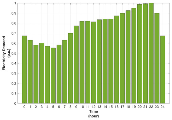
Figure 1.
Normalized load profile for an Italian household [15].
The simplified yearly load profile was then identified by repeating the daily load profile of Equation (2) along the whole year.
2.2. PV Production
The yearly PV production profile was calculated as a function of the PV size, solar irradiance and other factors (i.e., plant location, weather condition, etc.). As already mentioned, hourly data of solar radiation were obtained from PVGIS database, by means of API function [16], assuming PV modules with an optimal tilt angle and South facing. In particular, data were extracted for each cells of the raster up to cover the whole Country, by supposing the PV plants located in the centroids of the raster cells. Through the methodology presented in [19], the PV production profile can be finally calculated on hourly basis, as follows:
where is the hourly irradiance from PVGIS database, is the rated power of the PV plant, is the productivity loss factor to consider the yearly degradation of PV modules and is the performance ratio of PV system. The simplified approach of Equation (3) is derived by comparing the production of a PV module operating in real condition with the maximum (peak) production obtained during standard conditions (i.e., where G = 1000 W/m). Then, and were introduced to take into account PV module degradation, DC/AC conversion losses, cable losses and external temperature effects in the yearly production of PV plants. In particular, factor was assumed to increase linearly along years, as presented in [15].
2.3. Battery Management and Replacement
The integration of storage solutions within a PV plant introduces more flexibility in the system. Consequently, a management strategy for the battery must be identified in order to model how and when the storage should be used (i.e., how and when the battery should be charged or discharged), according to the PV production and the electricity demand. In this paper, the scheduling of the storage unit was implemented through an algorithm to evaluate and to manage the energy exchange with the battery, according to its operational limits. The proposed control strategy for the battery is based on the assumption that only a charge/discharge cycle per day can be acted in order to increase battery lifetime [20]. The following simplified scheduling was adopted:
- The battery is charged only with the PV overproduction. Otherwise, the battery can not be charged with electricity from the grid.
- The battery is discharged only when PV production is zero (i.e., during nighttime) to cover household demand. So, the discharge is avoided during daylight.
This simplified scheduling does not significantly affect the economic benefits of the storage. In fact, a flat tariff is assumed here for the electricity purchased from the grid. This is a common condition for residential end-users in Italy [21]. Under this assumption, battery discharge during nighttime has the same economic effect of a discharge during daytime. So, discharge during daylight can be potentially avoided increasing battery lifetime without impact on economic revenues.
Finally, the algorithm for the battery management verifies the energy balance of the storage at each time interval. Hence, the State of Charge () of the battery is calculated taking into account the charge/discharge efficiencies (i.e., and ) and the power flows through the battery, as follows [22]:
where and are the electricity injected into the battery and released by the storage, while and are the efficiency during charge and the discharge operation of the battery, respectively. Then, the is kept within an opportune operational interval, as follows:
The constraint of Equation (5) is needed to limit the level of Depth of Discharge () according to the battery technology [23]. In fact, it is worth noting that the minimum (i.e., ) and consequently the adopted should prevent capacity loss and degradation of battery lifetime due to high or unusual . Additionally, the power exchanged with the battery during the charge and the discharge were limited according to the full charge/discharge time of the battery and , as follows:
However, battery is affected by a degradation of its rated capacity and performances along the years. So, battery must be replaced when the number of discharge cycles reaches the battery’s cycle life (i.e., when the battery lifetime is reached) according to the adopted . For this reason, the number of yearly discharge cycles was calculated, as follows [24]:
The battery was replaced when the cumulative sum of the yearly discharge cycles is grater than the battery’s cycle life.
2.4. Battery Sizing
After the identification of a strategy for the battery management, the size of the storage system was also calculated on energy basis for different PV sizes and yearly household demand. In particular, the daily load profile was compared on hourly basis to the daily profile of the PV production over the whole year. Consequently, the electricity sold to the grid and the one purchased from the grid can be easily calculated for each day of the year and used to create two vectors:
where and are the vectors of the daily electricity sold to the grid and purchased from the grid, respectively. The battery size, or equivalently the maximum state of charge of the battery, was calculated by comparing these two vectors, as follows:
Under the assumption that battery is used to cover nighttime load demand (as presented in Section 2.3), Equation (11) ensures the following conditions:
- battery size is not overestimated when the higher possible PV overproduction occurs (i.e., battery is not underused during winter)
- battery size is not overestimated when the higher net electricity demand during nighttime occurs (i.e., battery is not underused during summer)
2.5. Household Energy Balance
Once the load profile, the PV size and the storage capacity were set, the electricity sold to the grid and the one purchased from the grid as well as the one self-consumed were calculated on hourly basis. This energy balance is fundamental, since the economic, energy and environmental indicators (described in the next sections) depend on how energy fluxes are exchanged within the household.
The hourly energy balance described by Equation (12) highlights that the storage unit is not used (i.e., and are zeros) during daytime, if PV production is lower than end-user demand , according to the rules described in Section 2.3. Consequently, the net load demand (i.e. the difference between demand and PV production) is covered by the electricity purchased from the grid .
Instead, when PV overproduction occurs during daytime (see Equation (13)), electricity is no longer purchased from the grid (i.e., ) and the energy surplus is stored in the battery (i.e., and ) until its maximum capacity is reached. Consequently, PV overproduction can be sold to the grid (i.e., ) only when battery is fully charged.
Finally, the battery can only be discharged (i.e., and ) when PV does not operate during nighttime (see Equation (14)), to cover the end-user demand down to its minimum SOC (i.e., ). When the storage is fully discharged (i.e., ) the load demand is totally covered by the electricity purchased from the grid.
It can be noticed that the described energy balance is based only on real power, even if reactive power can also be produced by the PV and battery inverter. However, the present Italian regulatory framework strongly limits the power factor within household. In this case, the production of reactive power is not taken into account, since the reactive power is assumed to be within the limits. Thus, no penalty has to be payed and the economic analysis is unaffected by reactive power production.
3. Economic Assumption
As already described, the energy model presented in Section 2 was used to identify the electricity flows within the household. Later, economic values were identified for each flow in order to perform the economic analysis of the PV and storage installation. In particular, the current electricity costs and revenues potentially gained by an Italian residential end-user were identified in this section.
3.1. Electricity Costs
The cost of the electricity purchased from the grid by a residential end-user is formed by different components in the Italian billing system: the energy cost, the access/grid costs and the taxes. The access and general system costs are formed by a fixed and a variable part. In particular, the yearly fixed costs are related to the installed capacity and to the number of the end-user connection points to the national grid , calculated as follows:
where and are the fixed access costs and the fixed general system costs. Differently, the yearly variable part of access/grid costs are related to the end-user electricity purchased from the grid , as follows:
where and are the variable access costs and the variable general system costs, respectively. Both fixed and variable parts of the access and general system costs are imposed and periodically updated by the Italian Regulatory Authority for Energy, Networks and Environment (ARERA).
In this context, the variable part of access and general system costs can be integrated into the energy cost to define an overall purchasing price which also includes the variable grid charges, as follows:
Consequently, the yearly cost for purchasing electricity from the grid can be calculated, as follows:
where taxes includes VAT and excises.
3.2. End-User Yearly Revenue
The installation of a PV system within an household converts the end-user into a prosumer, where PV production can be self-consumed and PV overproduction can be sold to the grid. Thus, the prosumer can gain an economic benefit from the PV production, that is defined as the difference between the cost to cover household demand without PV and the cost to cover the net household demand when PV is installed, as follows:
where is the net-metering contribution, while is the yearly operational and maintenance cost of the PV plant. In the Italian context, the additional net-metering contribution is an economic compensation mechanism based on the economic values of the energy injected into and purchased from the grid, which can be calculated as defined in [25,26,27]:
where is the economic value of the electricity taken from the grid to supply the household, is the economic value of the electricity sold to the grid, is the exchanged energy to the grid and S is an additional income. The is formed by three different contributions. The first term compensates, in whole or in part, the costs of the energy taken from the grid (see Equation (21)) with the economic value of the surplus energy produced by the PV plant and injected into the grid (see Equation (22)), where and are defined, as follows:
where is the reference national market price and is the reference zonal market price for energy injected into the grid. In this paper, a different price is assumed for each Italian region according to the six market zones of the National electricity market [28], as follows:
- North: Valle D’Aosta, Piemonte, Liguria, Lombardia, Trentino, Veneto, Friuli Venezia Giulia, Emilia Romagna.
- Northern-Central: Toscana, Umbria, Marche.
- Southern-Central: Lazio, Abruzzo, Campania.
- South: Molise, Puglia, Basilicata, Calabria.
- Sicily: Sicilia.
- Sardinia: Sardegna.
In particular:
- if < net-metering refunds the value of the whole energy purchased from the grid;
- if > net-metering refunds the value of energy produced by PV and injected into the grid (i.e., only a part of the energy purchased from the grid is refunded).
The second term of Equation (20) represents the contribution to refund the general system cost and the access cost for the exchanged energy , that is defined as follows:
where and are the energy purchased from the grid and the energy injected into the grid, respectively. The exchanged energy in Equation (23) is the electricity produced by PV plant and injected into the grid, which is subsequently taken from the grid to cover the household demand. The exchanged energy has an economic value measured through the coefficient , which is the weighted average value of the general system costs and the access costs.
The last term of Equation (20) represents the additional income S that can be further obtained if the economic value of the electricity produced by PV and injected into the grid is higher than the economic value of the electricity purchased from the grid. Substantially, the net-metering recovers this economic surplus which otherwise would be lost, as follows:
4. Economic, Environmental and Energy Indicators
The performances of a PV plant installed within an household were analyzed from the economic, energy and environmental point of view through different indicators. These indicators were also used to perform a comparison of the performances when different PV sizes and storage capacity were considered. In this section, the different indicators used in the analysis are presented and described.
4.1. Economic Indicators
The economic profitability of a PV plant with or without storage unit was based here on a cost-benefit analysis. In particular, the yearly costs and revenues, presented in the previous section, were used to calculate economic indicators to highlight the benefits of investing in PV plants with and without storage. Net Present Value (NPV), Internal Rate of Return (IRR), Discounted Pay Back Time (DPBT) and Levelized Cost of Energy (LCOE) are the economic indicators used here to evaluate the PV investment. The NPV is calculated as follows:
where N is the technical lifetime of the PV plant, d is the discount rate and is the tax deduction currently available in Italy for PV plant and storage unit. However, is a further benefit available only for small size residential installations. In fact, natural person (i.e., residential end-user) can recover 50% of the capital cost for installing a residential PV system, which can include a storage system, as tax deduction in a time span of ten years [3]. Equation (27) is also used to calculate the Discounted Pay Back Time (DPBT) for installing PV (with or without the integration of a battery system), since the DPBT is the period required to recover the initial capital expenditure . The Internal Rate of Return (i.e., the discount rate for which the NPV is equal to zero) is also calculated to evaluate the opportunity of the PV investment, as follows:
An IRR higher than the discount rate d reveals that the PV investment has an interest rate greater than an alternative investment, so it is potentially more attractive for investors. In addition, LCOE is also used to evaluate investment opportunity, since it defines the costs for RES electricity generation [29], as follows:
Typically, LCOE is compared either to the cost of the electricity purchased from the grid or to the generation cost of other alternative electricity sources. When LCOE is lower than the cost of the electricity purchased from the grid the so called “grid parity” is obtained.
Finally, an indicator of the cost saving for an end-user installing a PV system (with or without storage) is defined, as follows:
where is calculated as follows:
This indicator compares the overall costs for the End-User to buy electricity when PV system is installed with ones that were necessary if the whole electricity demand of end-user was taken from the grid (including VAT and excises).
4.2. Energy Indicators
The energy impact due to the installation of a PV system (with and without storage unit) within an household was analyzed through two different indicators: the self-consumption () and the self-sufficiency (). The former identifies the self-consumed PV production compared to the yearly PV production, while the latter identifies the self-consumed PV production compared to the yearly end-user demand, as follows [30]:
The values of these indicators depend on the match between the PV generation profile and the load profile of the household. In this paper, both hourly profiles were compared to analyze how and change according to different PV sizes and to different annual electricity household demand.
4.3. Environmental Indicator
Finally, the environmental impact of the PV installation was measured through the evaluation of the CO emission reduction (i.e., CO savings), calculated as follows:
where represents the national CO emission factor for the electricity purchased from the grid, as defined in [31]. Equation (34) compares the CO emissions due to the electricity purchased from the grid when PV is not installed (i.e., ), and the avoided emission due to the production of renewable energy by the PV. This indicator assumes that PV overproduction injected into the grid also contributes to the reduction of the CO emission, according to a global emission balance. In fact, the electricity sold to the grid reduces the need of producing electricity by the national thermoelectric power plants.
5. Results and Discussion
The aforementioned economic, energy and environmental analysis were performed considering different household consumption. In this paper two different yearly household electricity demand were assumed: 2700 kWp and 4000 kWh. The former represents the average consumption of an Italian residential end-user, while the latter represents the consumption of an household with an increased demand of 30% compared to the average one.
Once the energy demand is fixed, different sizes of the PV system were considered in a range from 1 kWp to 6 kWp, since the average size of PV installation for residential end-user is close to 4 kWp [4]. This PV size variation was considered to exploit PV potential in all the possible configurations taking also into account the integration of storage systems within households. As already described, the study presented here was performed subdividing the Italian territory at regional (i.e., NUTS2) level through a meshed grid with 2.5 × 2.5 km of resolution. Thus, a GIS approach was used to create a map with the same resolution, where hourly solar radiation data from JRC dataset [16] were assumed in each raster cell. Then the economic, energy and environmental analysis were performed in each cell within MATLAB environment by importing the raster map as a matrix. Table 1 highlights the main energy, economic and environmental parameters used to perform the analysis along the whole Italian context, while Table 2 summarizes the technical and operational characteristics of the battery considered in this study.

Table 1.
Energy economic and environmental parameters used for calculating indicators in each raster cell [19,20,31,32,33].
Table 2.
Main characteristics of the storage system considered in the study [20].
Finally, the national single price () and the zonal prices were extracted from [34] to measure the economic value of the electricity injected into the grid on hourly basis, as described in Section 3. In particular, a specific hourly zonal prices was considered for each administrative region, according to the six zones of the Italian electricity market.
A first result concerning the LCOE is shown in Figure 2. It can be noticed how the tax deduction supports the reduction of LCOE, since values lower than 200 €/MWh can be generally observed across Italy, making grid-parity closer also for residential end-user. The integration of battery storage solutions introduce benefits from the energy point of view. However, LCOE increases due to the still relevant unitary cost of storage system. In particular, LCOE get worse when the PV installed capacity increases, since the battery size and the corresponding investment costs increase as well.
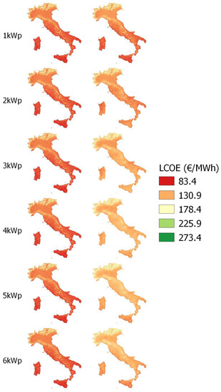
Figure 2.
Levelized Cost of Energy (LCOE) of photovoltaic (PV) sintallation, left side without battery and right side with battery.
In the next sections, results of the economic, environmental and energy analysis are presented and discussed for households with different yearly energy demand. Summary of the results are also presented in different tables at regional level by means of average values () and standard deviations (). Graphical representations of the economic, environmental and energy indicators are then reported in Appendix, through a series of colormaps.
5.1. Results = 2700 kWh without Battery
Results concerning the PV installation without battery are discussed in this section for an household with an electricity consumption corresponding to an average Italian residential end-user. As shown in Table 3 and Figure A2, CO savings in the range 40–60% are achievable at the lowest PV size. A stronger reduction of CO emission is expected for PV with an installed capacity of 6 kWp. In this case, savings up to 240–350% can be obtained due to the higher overproduction by renewable energy injected into the grid as confirmed by Table 4 and Table 5, where an increasing PV size reflects lower and unchanged .
Table 3.
CO saving for = 2700 kWh without battery.
Table 4.
Self-Consumption for = 2700 kWh without battery.
Table 5.
Self-Sufficiency for = 2700 kWh without battery.
Similar trends can be observed for the cost savings in Table 6 and Figure A3, where savings increase with the PV sizes. Typical costs saving ranges from 20–29% to 44–83% for an installed capacity of PV from 1 kWp to 6 kWp, respectively. Of course, a significant growth rate can be observed on cost saving for small PV size (i.e., 1–2 kWp), while a slightly growth rate is observed for higher PV size. This effect is due to the marginal impact of PV production with respect to the household energy demand, when PV sizes are higher (i.e., 5–6 kWp). In that case, self-consumption does not increase, so more PV overproduction is sold to the grid at selling price lower than the purchasing one .
Table 6.
Cost saving for = 2700 kWh without battery.
The Self-Consumption parameter decreases with increasing PV size (see Table 4 and Figure A7), showing how higher PV installed capacity increases the electricity injected into the grid. In facts, drops from 65–80% to 13–18% or an installed capacity of PV from 1 kWp to 6 kWp, respectively. This effect is more relevant in southern Italian regions with higher solar irradiance and higher PV production at fixed PV size.
Differently, an opposite trend occurs if Self-Sufficiency is considered (see Table 5 and Figure A8). In fact, higher PV sizes can potentially cover a larger part of the electrical load of the household. Thus, in the Italian territory, index can homogeneously range from 30–37% to 44–46% for PV sizes from 1 kWp to 6 kWp, respectively. However, the growth rate of decreases at higher PV size, since more electricity overproduction is expected.
Table 7 and Figure A4 show how the IRR lowers from about 1–3% to −2.5/−6% for PV sizes from 1 kWp to 6 kWp, respectively. The NPV shows a similar trend (see Table 8 and Figure A5), since it decreases from 154–470 € to −2044/−4580 € for PV sizes form 1 kWp to 6 kWp, respectively. Similarly, Table 9 and Figure A6 show that DPBT is also affected by the PV size. The economic return on PV investment can be expected within the range of 13–18 years at lower installed capacity of PV and in the southern Italian regions. In particular, Southern regions with higher yearly solar irradiation show positive economic profitability, since DPBT is lower than PV lifetime (i.e., 25 years) for installed capacity up to 2 kWp, with Sicily that can be attractive for investors up to 3 kWp. Otherwise, DPBT greater than PV lifetime (i.e., 25 years) can be observed in all the Italian regions for installed capacity higher than 4 kWp.
Table 7.
Internal Rate of Return (IRR) = 2700 kWh without battery.
Table 8.
Net Present Value (NPV) for = 2700 kWh without battery.
Table 9.
Discounted Pay Back Time (DPBT) for = 2700 kWh without battery.
5.2. Results = 2700 kWh with Battery
Results concerning the PV installation with battery are discussed in this section for an household with an electricity consumption corresponding to an average Italian residential end-user. As shown in Figure A1, the storage capacity calculated by adopting the sizing proposed in Section 2.4, it is strongly influenced by the PV peak power. In fact, small PV size can not have sufficient overproduction to be stored, hence bringing battery capacity to be lower. In contrast, battery size increases up to 4 kWh when PV size is grater than 3 kWp in Southern regions where higher solar irradiance is available.
Table 10 and Figure A2 show that the use of a storage system has a small influence on CO saving, since ita can range from 38–56% to 235–333% for PV sizes from 1 kWp to 6 kWp, respectively. Instead, the cost savings (see Table 11 and Figure A3) increase with respect to a configuration without storage. In fact, savings from 23–31% to 53–102% can be obtained by increasing PV size from 1 kWp to 6 kWp. It can be noticed that the cost saving can be greater than 100% in some cases, since PV overproduction can be sold to the grid and net-metering option is available.
Table 10.
CO saving for = 2700 kWh with battery.
Table 11.
Cost saving for = 2700 kWh with battery.
From the energy point of view, the results of Self-Consumption and Self-Sufficiency factors (see Table 12 and Table 13 and Figure A7 and Figure A8) clearly show how battery use introduce significant benefits. In fact, increases with respect to the configuration without storage. This is due to the possibility to self-consume the stored PV overproduction instead of selling it into the electric grid. For this reason, can range from 70–83% to 25–29% for installed capacities of PV ranging from 1 kWp to 6 kWp, respectively. Conversely, appears not influenced by the storage (i.e., ranges from 30% to 37%) for small PV size (i.e., small battery size), while is almost double (i.e., ranges from 61% to 81%) at higher PV size (i.e., at 6 kWp).
Table 12.
Self-Consumption for = 2700 kWh with battery.
Table 13.
Self-Sufficiency for = 2700 kWh with battery.
From an economic point of view, investment costs increase due to the capital cost of the battery system to be integrated within the plant. Consequently, the IRR (see Table 14 and Figure A4) range from 1–7% to −4.6/−7%, showing an increase if compared to the previous scenario without storage.
Table 14.
IRR = 2700 kWh with battery.
Moreover, results in Table 15 and Figure A5 indicate that the introduction of storage increases the NPV for small PV sizes (i.e., 200–1240 € is obtained at 1 kWp). While NPV decreases for higher PV size and battery in all the Italian regions. In fact, NPV lower than −4500 € can be observed in most of the cases where installed capacity of PV is greater than 4 kWp.
Table 15.
NPV for = 2700 kWh with battery.
Finally, if a storage unit is integrated within the PV plant, the DPBT decreases for small PV size, due to higher self-consumed energy (see Table 16 and Figure A6). Otherwise the economic profitability of the storage is lost when PV size is greater than 3 kWp, since no regions seem to allow acceptable investment payback time.
Table 16.
DPBT for = 2700 kWh with battery.
5.3. Results = 4000 kWh without Battery
Results concerning the PV installation without battery are discussed in this section for an household with an electricity consumption increased with respect to an average Italian residential end-user. This context was explored to consider also residential end-user with an higher attitude in electricity consumption.
From the economic point of view, Table 17 and Figure A12 show that IRR lowers from about 3–9% to −1% for PV sizes ranging from 1 kWp to 6 kWp, respectively. Similarly, the NPV shows a trend (see Table 18 and Figure A13) where it can ranges from 560/1600 € down to around −1220/−1320 € for PV sizes from 1 kWp to 6 kWp, respectively. Table 19 and Figure A14 finally show that DPBT is still influenced by the PV size ranging from around 7 years to values grater than the PV lifetime. However, household with an increased energy consumption can obtain more benefits from an economic perspective, since PV production can be largely self-consumed. In fact, the comparison of these economic results with ones at lower yearly consumption (i.e., 2700 kWh), reveals that economic performances are better for households with higher demand. These benefits are even better for southern Italian regions with higher availability of solar radiation.
Table 17.
IRR for = 4000 kWh without battery.
Table 18.
NPV for = 4000 kWh without battery.
Table 19.
DPBT for = 4000 kWh without battery.
From the environmental point of view, CO savings range from 30% to 40% for small PV size (i.e., 1 kWp), as shown in Table 20 and Figure A10. However, a strong increase up to 164–242% can be obtained for higher PV size (i.e., 6 kWp), due to the higher PV production.
Table 20.
CO saving for = 4000 kWh without battery.
Instead, Table 21 and Figure A11 show how cost savings can range from 15–24% to 49–67% for PV sizes ranging from 1 kWp to 6 kWp, respectively. Once again, higher costs saving can be observed in southern regions due to higher availability of solar radiation. In addition, as already pointed out for the other economic indicators, households with higher yearly consumption (i.e., 4000 kWh) can also obtain higher cost savings compared to ones with lower yearly consumption (i.e., 2700 kWh).
Table 21.
Cost saving for = 4000 kWh without battery.
From the energy point of view, the Self-Consumption decreases with increasing PV size. This trend shows how higher PV size increases the energy that can be injected into the grid and not self-consumed (see Table 22 and Figure A15). In facts, drops from 84–95% (at 1 kWp) to 19–27% (at 6 kWp). Finally, Self-Sufficiency shows an opposite trend with respect to (see Table 23 and Figure A16). In fact, can range from 25–33% to 42–45% when PV size ranges from 1 kWp to 6 kWp.
Table 22.
Self-Consumption for = 4000 kWh without battery.
Table 23.
Self-Sufficiency for = 4000 kWh without battery.
5.4. Results = 4000 kWh with Battery
Results concerning the PV installation with battery are discussed in this section for an household with an electricity consumption (i.e., 4000 kWh) increased with respect to an average Italian residential end-user. As shown in Figure A9, the storage capacity calculated by adopting the sizing proposed in Section 2.4, it is strongly influenced by the PV peak power. In fact, as already observed for the scenario with 2700 kWh of yearly demand, small PV size can not have sufficient overproduction to be stored, hence bringing battery capacity to be lower.
In this scenario, Self-Consumption still decreases with increasing PV sizes (see Table 24 and Figure A15). In particular, almost all the PV production can be self-consumed in configurations with small PV sizes. Conversely, PV sizes above 3 kWp inject part of the energy produced into the grid. However, benefits can be obtained from the energy point of view, when a storage system is integrated. In fact, increases, if compared to the configuration without storage, showing ranges from 88–96% to 30–36% for PV size from 1 kWp to 6 kWp, respectively. This is still due to the possibility to self-consume the stored PV overproduction, which otherwise would be sold to the grid.
Table 24.
Self-Consumption for = 4000 kWh with battery.
On the other hand, seems not influenced by the storage in configuration with small PV sizes (see Table 25 and Figure A16), since it ranges from 23% to 32%. While battery can almost double the at higher PV size. In fact, ranges from 50% to 78% for PV size of 6 kWp.
Table 25.
Self-Sufficiency for = 4000 kWh with battery.
The environmental impact decreases with increasing PV size (i.e., the CO emission decreases), as already observed for the scenario with 2700 kWh of yearly demand. However, Table 26 and Figure A10 shows that the storage system has a limited influence on CO saving. Indeed, CO savings range from 25.69–37.95% to 152–223% for PV size from 1 kWp to 6 kWp, respectively. But these results are close to ones observed for the scenario without storage system.
Table 26.
CO saving for = 4000 kWh with battery.
Finally, the trends of the economic indicators appear similar to those obtained for the scenario an yearly demand of 2700 kWh. Cost savings (see Table 27 and Figure A11) are comparable with ones obtained for the scenario without storage: cost saving ranges from 17–27% to 57–82% for PV size ranging from 1 kWp to 6 kWp. The IRR (see Table 28 and Figure A12) ranges from 3–8% (at 1 kWp) to −1/−5% (at 6 kWp), showing an increasing trend with respect to the scenario without battery system. Results in Table 29 and Figure A13 indicate that the integration of storage increases the NPV for small PV size (588–1561 € at 1 kWp), but economic benefits decreases with increasing PV and battery size. Finally, DPBT increases for higher PV size, since battery size increase with increasing PV size and higher investment cost are thus expected (see Table 30 and Figure A14). As a result, the economic convenience of the storage is lost for configurations with an installed PV capacity greater than 3 kWp. In fact, higher PV sizes show investment payback time greater than the PV technical lifetime.
Table 27.
Cost saving for = 4000 kWh with battery.
Table 28.
IRR for = 4000 kWh with battery.
Table 29.
NPV for = 4000 kWh with battery.
Table 30.
DPBT for = 4000 kWh with battery.
6. Conclusions
The study presented in this paper aiming at investigating how renewable solar energy can be exploited by households, through a detailed economic, energy, and environmental analysis for the whole of Italy, considering the current regulatory framework (i.e., including tax deduction for renewable installation) and the integration of storage systems. The analysis was performed through an hourly-based energy balance considering PV production with different PV sizes and different household energy demands. The investigation was implemented through a GIS (Geographical Information System) approach, where the whole Italian territory is represented by a meshed grid with a resolution of 2.5 × 2.5 km (i.e., formed by raster cells).
This approach investigates investment profitability as well as energy and environmental benefits for grid-connected PV systems with and without storage systems in large areas, where the yearly amount of available solar energy resource changes according to the plant location within the meshed grid. Results were measured by energy, economic and environmental indicators for each raster cell, considering both 2700 kWh and 4000 kWh yearly energy demand for Italian households.
The main outline of this paper is twofold:
- without storage, the DPBT in a scenario with a yearly demand of 2700 kWh seems to be globally lower than PV lifetime just for PV size lower than 2 kWp. Furthermore, the average IRR remains positive (i.e., around 1.85%) only for small PV sizes (i.e., 1 kWp). On the other hand, for a yearly consumption of 4000 kWh, the DPBT can still be within the range of 11–17 years for PV sizes up to 4 kWp. Besides, all Italian regions show positive IRR for PV sizes up to 4 kWp, with a maximum (i.e. around 6.3%) for the smallest one (i.e., 1 kWp). Hence, it can be concluded that scenarios with larger energy demand are more suitable for PV installation from an economic point of view, since an increase of and a decrease of are observed. From the energy point of view, the decreases with increasing PV size from 72% to 16% for 2700 kWh yearly demand and from 90% to 23% for 4000 kWh yearly consumption. So, higher are expected in households with higher demand due to a larger self-consumption of PV production.
- with storage, the renewable energy self-consumed by the residential end-user can be further increased. PV overproduction can be stored instead of selling it into the grid and the battery can be discharged when PV production is absent (i.e., during nighttime). As a result, higher self-consumption can be obtained, if compared to the scenarios without storage, since the ranges from 76% to 27% at 2700 kWh yearly demand, while it ranges from 93% to 34% at 4000 kWh yearly consumption. The storage systems also lead to an increase of , especially at high PV sizes. increases from 45% to 73% in a scenario with a yearly consumption of 2700 kWh and a PV size of 6 kWp. The same increase is observed in a scenario with a yearly consumption of 4000 kWh where passes from 44% to 63%. On the other hand, installation of a battery system raises investment costs, so that DPBT worsens due to the still high battery cost and IRR lowered as well.
Environmental benefits were also investigated, showing that PV production reduces greenhouse gas emissions up to 203% considering the self-consumption effect and the injection of PV overproduction into the grid.
Additionally, it can be concluded that the integration of storage within a PV installation improves the energy performance of the system due to the increased ability of the user to be independent of the electric grid. On the other hand, the use of battery systems increases system costs, so that only smaller PV sizes remain attractive to investors from an economic point of view. A reduction in storage costs could further boost the installation of renewable energy plants.
Future works may involve energy analysis with larger energy demands considering the electrification of other energy vectors as a target to be combined with renewable energy sources. According to this paper, huge energy consumption seems to make photovoltaic and/or storage systems attractive from energy, economic and environmental points of view. In this context, Renewable Energy Communities (REC) or Collective Self-Consumption Communities, introduced by the EU Renewable Energy Directive 2018/2001 [35] (also known as RED II), can represent an opportunity as a cluster of domestic users (for example, a condominium) equipped with a PV plant to maximize global self-consumption.
Author Contributions
Conceptualization, P.L.; Data curation, M.Q. and I.M.; Formal analysis, P.L., M.Q. and I.M.; Methodology, P.L. and M.R.; Software, P.L., M.Q. and I.M.; Writing original draft, P.L., M.Q. and I.M.; Writing, review & editing, P.L. and M.R. All authors have read and agreed to the published version of the manuscript.
Funding
This research received no external funding.
Institutional Review Board Statement
Not applicable.
Informed Consent Statement
Not applicable.
Data Availability Statement
Publicly available datasets were analyzed in this study. This data can be found here: https://ec.europa.eu/jrc/en/PVGIS/docs/noninteractive.
Conflicts of Interest
The authors declare no conflict of interest.
Abbreviations
The following abbreviations are used in this manuscript:
| economic value of the electricity produced and injected into the grid | |
| price of electricity bought from the grid excluding grid costs | |
| price of electricity bought from the grid including grid costs | |
| price of electricity sold to the grid | |
| investment cost for PV plant | |
| investment cost for battery | |
| weighted average value of the general system costs and access costs for the end-user | |
| d | discount rate |
| depth of charge of the battery | |
| DPBT | discounted pay-back time of the investment (years) |
| yearly electricity exchanged with the grid | |
| yearly end-user energy consumption | |
| yearly energy bought from the grid | |
| yearly energy sold to the grid | |
| hourly solar irradiance at optimum tilt and south facing | |
| IRR | internal rate of return |
| LCOE | levelized cost of energy |
| N | technical lifetime of PV modules |
| net-metering contribution | |
| NPV | net present value |
| economic value of the electricity bought from the grid | |
| operational costs for PV plant | |
| peak power of the PV plant | |
| percentage of the energy cost reduction for the end-user | |
| productivity loss of PV module | |
| performance ratio of the PV plant | |
| S | additional net-metering income for PV energy surplus |
| self-consumption | |
| state of charge of the battery | |
| self-sufficiency | |
| tax deduction of PV installation | |
| yearly cost for the end-user | |
| yearly energy supply cost for the end-user | |
| yearly revenues |
Appendix A
In this section, the results presented and discussed in Section 5 are graphically shown as a series of colormaps, each one representing the investigated energy, economic and environmental indicators for the whole Italian country. For each indicator, the comparison between storage and no-storage configuration can be graphically observed from Figure A1, Figure A2, Figure A3, Figure A4, Figure A5, Figure A6, Figure A7, Figure A8, Figure A9, Figure A10, Figure A11, Figure A12, Figure A13, Figure A14, Figure A15 and Figure A16 by considering different PV size and different yearly household electricity demand.

Figure A1.
Battery size for = 2700 kWh.

Figure A2.
CO saving for = 2700 kWh, left side without battery and right side with battery.

Figure A3.
Cost saving for = 2700 kWh, left side without battery and right side with battery.

Figure A4.
IRR for = 2700 kWh, left side without battery and right side with battery.

Figure A5.
NPV for = 2700 kWh, left side without battery and right side with battery.

Figure A6.
DPBT for = 2700 kWh, left side without battery and right side with battery.

Figure A7.
SC for = 2700 kWh, left side without battery and right side with battery.

Figure A8.
SS for = 2700 kWh, left side without battery and right side with battery.

Figure A9.
Battery size for = 4000 kWh.

Figure A10.
CO saving for = 4000 kWh, left side without battery and right side with battery.

Figure A11.
Cost saving for = 4000 kWh, left side without battery and right side with battery.

Figure A12.
IRR for = 4000 kWh, left side without battery and right side with battery.

Figure A13.
NPV for = 4000 kWh, left side without battery and right side with battery.

Figure A14.
DPBT for = 4000 kWh, left side without battery and right side with battery.

Figure A15.
SC for = 4000 kWh, left side without battery and right side with battery.

Figure A16.
SS for = 4000 kWh, left side without battery and right side with battery.
References
- IEA. CO2 Emissions from Fuel Combustion. 2020. Available online: https://www.iea.org/reports/co2-emissions-from-fuel-combustion-overview (accessed on 8 January 2021).
- IEA. Empowering Electricity Consumers to Lower Their Carbon Footprint. 2020. Available online: https://www.iea.org/commentaries/empowering-electricity-consumers-to-lower-their-carbon-footprint (accessed on 8 January 2021).
- Cucchiella, F.; D’Adamo, I.; Gastaldi, M. Economic Analysis of a Photovoltaic System: A Resource for Residential Households. Energies 2017, 10, 814. [Google Scholar] [CrossRef]
- GSE. Solare Fotovoltaico–Rapporto Statistico. 2020. Available online: https://www.gse.it/documenti_site/Documenti%20GSE/Rapporti%20statistici/Solare%20Fotovoltaico%20-%20Rapporto%20Statistico%202019.pdf (accessed on 8 January 2021).
- Gomez-Gonzalez, M.; Hernandez, J.; Vera, D.; Juradoa, F. Optimal sizing and power schedule in PV household-prosumers for improving PV self-consumption and providing frequency containment reserve. Energy 2020, 191, 116554. [Google Scholar] [CrossRef]
- Hernandez, J.; Sanchez-Sutil, F.; Muñoz-Rodríguez, F.J.; Baier, C.R. Optimal sizing and management strategy for PV household-prosumers with self-consumption/sufficiency enhancement and provision of frequency containment reserve. Appl. Energy 2020, 277, 115529. [Google Scholar] [CrossRef]
- Aniello, G.; Shamon, H.; Kuckshinrichs, W. Micro-economic assessment of residential PV and battery systems: The underrated role of financial and fiscal aspects. Appl. Energy 2021, 281, 115667. [Google Scholar] [CrossRef]
- Elkazaz, M.; Sumner, M.; Pholboon, S.; Davies, R.; Thomas, D. Performance Assessment of an Energy Management System for a Home Microgrid with PV Generation. Energies 2020, 13, 3436. [Google Scholar] [CrossRef]
- Candelise, C.; Westacott, P. Can integration of PV within UK electricity network be improved? A GIS based assessment of storage. Energy Policy 2017, 109, 694–703. [Google Scholar] [CrossRef]
- Walch, A.; Castello, R.; Mohajeri, N.; Scartezzini, J. Big Data mining for the estimation of hourly rooftop photovoltaic potential and its uncertainty. Appl. Energy 2020, 262. [Google Scholar] [CrossRef]
- Colak, H.; Memisoglu, T.; Gercek, Y. Optimal site selection for solar photovoltaic (PV) power plants using GIS and AHP: A case study of Malatya Province, Turkey. Renew. Energy 2020, 149, 565–576. [Google Scholar] [CrossRef]
- Pillot, B.; Al-Kurdi, N.; Gervet, C.; Linguet, L. An integrated GIS and robust optimization framework for solar PV plant planning scenarios at utility scale. Appl. Energy 2020, 260, 114257. [Google Scholar] [CrossRef]
- Camilo, F.M.; Castro, R.; Almeida, M.E.; Pires, V.F. Economic assessment of residential PV systems with self-consumption and storage in Portugal. Sol. Energy 2017, 150, 353–362. [Google Scholar] [CrossRef]
- Cerino Abdin, G.; Noussan, M. Electricity storage compared to net metering in residential PV applications. J. Clean. Prod. 2018, 176, 175–186. [Google Scholar] [CrossRef]
- Lazzeroni, P.; Moretti, F.; Stirano, F. Economic potential of PV for Italian residential end-users. Energy 2020, 200C, 117508. [Google Scholar] [CrossRef]
- PVGIS—European Communities. Non-Interactive Service. 2020. Available online: https://ec.europa.eu/jrc/en/PVGIS/docs/noninteractive (accessed on 8 January 2021).
- Alabito, M. Contributo Delle Elettrotecnologie per usi Finali al Carico di Punta; Technical Report. 2005. Available online: https://www.rse-web.it/documenti.page?RSE_originalURI=/documenti/documento/311943&RSE_manipulatePath=yes&country=ita (accessed on 8 January 2021).
- Liddo, P.D.; Lazzeroni, P.; Olivero, S.; Repetto, M.; Ricci, V.A. Application of Optimization Procedure to the Management of Renewable Based Household Heating & Cooling Systems. Energy Procedia 2014, 62, 329–336. [Google Scholar] [CrossRef][Green Version]
- Lazzeroni, P.; Olivero, S.; Repetto, M. Economic perspective for PV under new Italian regulatory framework. Renew. Sustain. Energy Rev. 2017, 71, 283–295. [Google Scholar] [CrossRef]
- Minuto, F.D.; Lazzeroni, P.; Borchiellini, R.; Olivero, S.; Bottaccioli, L.; Lanzini, A. Modeling technology retrofit scenarios for the conversion of condominium into an energy community: An Italian case study. J. Clean. Prod. 2020, 124536. [Google Scholar] [CrossRef]
- ARERA. Relazione Annuale Sullo Stato dei Servizi e Sull’attivita’ Svolta. 2020. Available online: https://www.arera.it/allegati/relaz_ann/20/RA20_volume1.pdf (accessed on 8 January 2021).
- Lazzeroni, P.; Repetto, M. Optimal planning of battery systems for power losses reduction in distribution grids. Electr. Power Syst. Res. 2019, 167, 94–112. [Google Scholar] [CrossRef]
- Letcher, T. Storing Energy with Special Reference to Renewable Energy Sources; Elsevier: Amsterdam, The Netherlands, 2016. [Google Scholar]
- Debarberis, L.; Lazzeroni, P.; Olivero, S.; Ricci, V.A.; Stirano, F.; Repetto, M. Technical and economical evaluation of a PV plant with energy storage. In Proceedings of the 39th Annual Conference of the IEEE Industrial Electronics Society (IECON), Vienna, Austria, 10–13 November 2013. [Google Scholar] [CrossRef]
- Testo Integrato Delle Modalità e Delle Condizioni Tecnico-Economiche per L’erogazione del Servizio di Scambio sul Posto. Deliberazione 570/2012/r/efr, 20 Dicembre 2012. Available online: https://www.arera.it/allegati/docs/08/074-08argall.pdf (accessed on 8 January 2021).
- Attuazione Delle Disposizioni del Decreto Legge 91/14 in Materia di Scambio sul Posto. Deliberazione 612/2014/r/eel, 11 Dicembre 2014. Available online: https://www.arera.it/allegati/docs/14/612-14.pdf (accessed on 8 January 2021).
- GSE. Servizio di Scambio sul Posto. Determinazione del Contributo in conto Scambio ai Sensi Dell’articolo 12 Dell’Allegato A alla Deliberazione 570/2012/R/efr e s.m.i.–Regole Tecniche; Gestore dei Servizi Energetici S.p.A: Roma, Italy, 2019. [Google Scholar]
- GME. Italian Electricity Market Zones. 2020. Available online: http://www.mercatoelettrico.org/en/mercati/mercatoelettrico/zone.aspx (accessed on 8 January 2021).
- Braker, K.; Pathak, M.; Pearce, J. A review of solar photovoltaic levelized cost of electricity. Renew. Sustain. Energy Rev. 2011, 15, 4470–4482. [Google Scholar] [CrossRef]
- IEA. Photovoltaic Power Systems Programme—A Methodology for the Analysis of PV Self-Consumption Policies. 2016. Available online: https://iea-pvps.org/wp-content/uploads/2020/01/IEA-PVPS_-_A_methodology_for_the_Analysis_of_PV_Self-Consumption_Policies.pdf (accessed on 8 January 2021).
- ISPRA. Fattori di Emissione Atmosferica di gas a Effetto Serra nel Settore Elettrico Nazionale e nei Principali Paesi Europei. 2019. Available online: https://www.isprambiente.gov.it/it/pubblicazioni/rapporti/fattori-di-emissione-atmosferica-di-gas-a-effetto-serra-nel-settore-elettrico-nazionale-e-nei-principali-paesi-europei (accessed on 8 January 2021).
- Energy and Strategy Group. Renewable Energy Report; Technical Report; Politecnico di Milano: Milan, Italy, 2018. [Google Scholar]
- ARERA. Deliberazione 25 Gennaio 2018 32/2018/R/efr—Determinazione del Valore Medio del Prezzo di Cessione Dell’energia Elettrica Dell’anno 2017, ai fini Della Quantificazione, per L’anno 2018, del Valore Degli Incentivi Sostitutivi dei Certificati Verdi. 2018. Available online: https://www.arera.it/it/docs/18/032-18.htm (accessed on 8 January 2021).
- Gestore Mercati Energetici—GME. Available online: http://www.mercatoelettrico.org/en/Default.aspx (accessed on 8 January 2021).
- Promotion of the Use of Energy from Renewable Sources. Directive (EU) 2018/2001 of the European Parliament and of the Council, 11 December 2018. Available online: https://eur-lex.europa.eu/legal-content/EN/TXT/?uri=LEGISSUM%3Aen0009 (accessed on 8 January 2021).
Publisher’s Note: MDPI stays neutral with regard to jurisdictional claims in published maps and institutional affiliations. |
© 2021 by the authors. Licensee MDPI, Basel, Switzerland. This article is an open access article distributed under the terms and conditions of the Creative Commons Attribution (CC BY) license (http://creativecommons.org/licenses/by/4.0/).