Meta-Heuristic Optimization Techniques Used for Maximum Power Point Tracking in Solar PV System

Abstract

A critical advancement in solar photovoltaic (PV) establishment has led to robust acceleration towards the evolution of new MPPT techniques. The sun-oriented PV framework has a non-linear characteristic in varying climatic conditions, which considerably impact the PV framework yield. Furthermore, the partial shading condition (PSC) causes major problems, such as a drop in the output power yield and multiple peaks in the P–V attribute. Hence, following the global maximum power point (GMPP) under PSC is a demanding problem. Subsequently, different maximum power point tracking (MPPT) strategies have been utilized to improve the yield of a PV framework. However, the disarray lies in choosing the best MPPT technique from the wide algorithms for a particular purpose. Each algorithm has its benefits and drawbacks. Hence, there is a fundamental need for an appropriate audit of the MPPT strategies from time to time. This article presents new works done in the global power point tracking (GMPPT) algorithm field under the PSCs. It sums up different MPPT strategies alongside their working principle, mathematical representation, and flow charts. Moreover, tables depicted in this study briefly organize the significant attributes of algorithms. This work will serve as a reference for sorting an MPPT technique while designing PV systems.

1. Introduction

Reserves of natural fossil fuels are getting depleted at a rapid pace. Therefore, the growing electricity demand can be met by employing renewable energy sources. Renewable energy sources show potential avenues for electricity generation. Among various sustainable energy sources, solar energy proves to be a viable substitute for electricity generation, since it is an ample, inexhaustible, and non-polluting source of energy.

Solar energy production is booming at a fast rate. This growth is due to the recent advancements in accuracy, convergence speed for harvesting maximum energy [1,2]. As suggested by the International Energy Agency report ‘Global Energy Review 2021’, global electricity demand is due to increase by 4.5% in 2021, or more than 1000 TWh. In 2020, renewable energy grew by 3%. Furthermore, the demand for renewable energy will increase in 2021 in every sector, such as heating, power, etc. Sun-powered photovoltaic (PV) and wind are estimated to be a factor of two-thirds of renewable development. The contribution of renewable energy sources in electricity production will grow practically by 30% in 2021, indicating the highest share of renewable energy sources since the Industrial Revolution. Therefore, Solar PV electricity production is likely to ascend by 145 TWh, or practically by 18% in 2021.

A solar cell produces DC power when solar rays incident on it. Therefore, several solar cells are connected to form a PV module. Later, the grouping of solar modules results in the formation of the solar array. PV modules have relatively low conversion efficiency due to the nonlinear characteristics of the solar cells. Therefore, it becomes necessary to exploit the maximum available power from the PV modules.

Moreover, the maximum power supplied by the photovoltaic module is not static as the atmospheric parameters such as irradiance level, temperature, dirt, and the particular installing conditions, such as the geographical conditions of an area, influence the performance of a PV system [3]. Hence, there is a need to investigate studies related to forecasting weather conditions precisely as solar energy is available free of cost in nature. So, PV systems can either be a grid-connected generating unit or a standalone generating unit. Therefore, rural areas and poor grid power quality regions get electricity from such units [4].

The P–V characteristics of the solar cell exhibit an optimum point that varies under atmospheric conditions (i.e., solar irradiance and temperature). At that point, the cell generates the maximum power. Consequently, the maximum power point tracking (MPPT) technique is employed to ensure that the photovoltaic (PV) module exploits optimum capacity at all times [5].

In the last decade, various MPPT methodologies were suggested to extract the maximum power from the PV modules [6]. However, the selection of a particular method is still obscure. Moreover, until now, recent research works do not include all newly developed MPPT algorithms. Therefore, there is a great need to analyze and review the proposed strategies from time to time, which will provide an insight into the selection of specific methods as per the context.

In this article, different MPPT techniques have been reviewed and then compared on the basis of several factors such as tracking speed, cost of implementation, complexity, etc. These MPPT techniques can be classified into two significant groups, specifically, conventional and meta-heuristic strategies. Conventional techniques comprise perturb and observe (P&O), incremental conductance, fractional open-circuit voltage, and fractional short circuit currents. Meta-heuristic strategies reassessed include swarm-intelligence (SI) and bio-inspired (BI). SI consists of the particle swarm optimization (PSO), ant colony optimization (ACO), artificial bee colony (ABC), grey wolf optimization (GWO), emperor penguin optimization (EPO), salp swarm algorithm (SSA), and jaya algorithm (JA). BI comprises cuckoo search (CS), flying squirrel search optimization (FSSO), owl search algorithm (OSA), and firefly algorithm (FFA). Whereas artificial intelligence (AI) techniques include fuzzy logic control (FLC), artificial neural networks (ANN), and its sub-categorization evolutionary computational (EC). EC strategies studied consist of a genetic algorithm (GA) and differential evolution (DE).

This article is structured as follows: Section 2 explains the Solar cell characteristic. The influence of environmental factors on the I–V and P–V curves is discussed in Section 3. Section 4 introduces the equivalent circuit diagram of the solar cell. Section 5 discusses the partial shading effect. In Section 6, MPPT algorithms and their categorization are discussed. Section 7 presents a comparison between the MPPT techniques along with their merits and demerits. Section 8 covers the simulation results of the implemented algorithm under partial shading conditions (PSC). The future scope of the research work is discussed in Section 9. Lastly, Section 10 concludes the work with some operable viewpoints.

2. Equivalent Circuit Model of Solar Cell

The simple single diode model represents the PV cell. The equivalent single diode circuit consists of a diode, a current source, a shunt resistor, and a series resistor. Primarily, an ideal solar cell is modeled by a current source in parallel with a diode. For practical applications, the model incorporates series resistance and shunt resistance. Generally, in the equivalent model of the solar cell, the shunt resistance (R_sh) signifies manufacturing defects and poor solar cell design, while the series resistance (R_s) accounts for the contact resistances [7]. The fundamental single-diode model of the PV cell is illustrated in Figure 1.

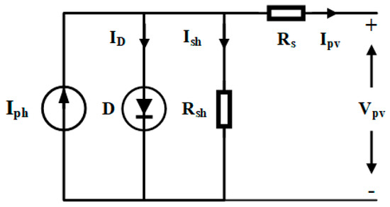
Figure 1. Single diode model of the solar cell.

The current produced by the solar cell is given by Equation (1).

$$I_{pv}=I_{ph}-I_D-I_{sh}$$

(1)

where I_pv represents output current; I_ph indicates the photoelectric current; I_D denotes the diode current; I_sh signifies the shunt current.

To compute current flowing in the diode, utilize the Shockley equation as per Equation (2).

$$I_D=I_0\left[exp\left(\frac{q}{nkT}\left(V_{pv}+I_{pv} R_S\right)\right)-1\right]$$

(2)

By Ohms law, the current flowing in the shunt resistor, I_sh, is calculated by using Equation (3).

$$I_{sh}=\frac{ V_{pv}+I_{pv}{R}_S}{R_{sh}}$$

(3)

The characteristic equation of a solar cell is specified in Equation (4).

$$I_{pv}=I_{ph}-I_0\left[exp\left(\frac{q}{nkT}\left(V_{pv}+I_{pv} R_S\right)\right)-1\right]-\frac{V_{pv}+I_{pv}{R}_S}{R_{sh}}$$

(4)

where I_ph signifies the photoelectric current, q denotes the electron charge; I₀ represents the reverse saturation current of the diode; V_pv indicates the voltage across the diode; R_s and R_sh represent the series and shunt resistors of the solar cell in (Ω), respectively; T denotes the temperature at the junction; K means the Boltzmann’s constant [4]; n signifies the ideality factor of the diode.

3. Solar Cell Characteristic

The short circuit current (I_sc) stands for the current flow in the short-circuit condition of the solar cell. The open-circuit voltage (V_oc) signifies the maximum voltage available from the solar cell during the open-circuit condition. However, short circuit and open circuit conditions do not contribute to power generation. Nevertheless, a specific combination of voltage and current led to maximum power (P_max) generation. The coordinates of the combination indicate the maximum power point (MPP). I–V and P–V curves of the solar cell are exhibited in Figure 2.

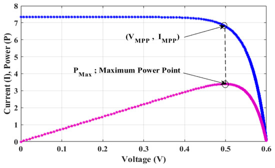
Figure 2. The I–V and P–V characteristic curves of the solar cell.

4. Influence of Environmental Factors on I–V and P–V Characteristic Curves

4.1. Effect of Varying Temperature on I–V and P–V Characteristicsof the Solar Cell

Temperature change shows a significant impact on the performance of the module. The effect of change in temperature on the P–V and I–V curves is demonstrated in Figure 3 and Figure 4, respectively. The variation in temperature from 25 °C to 125 °C is studied. Furthermore, from Figure 3, it can be concluded that the open-circuit voltage (V_oc) of the PV module decreases with the increase in temperature. As a result, the output power yield of the PV module will drop.

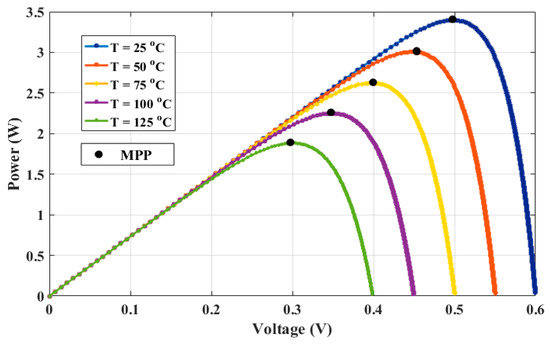
Figure 3. The influence of varying the temperature on the P–V characteristics of the solar cell.

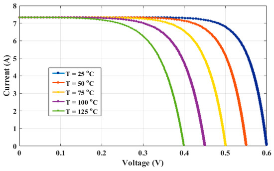
Figure 4. The effect of varying the temperature on the I–V characteristics of the solar cell.

4.2. Effect of Varying Insolation on I–V and P–V Characteristicsof the Solar Cell

The effect of change of insolation on the I–V and P–V curve is observed by varying the insolation from 200 W/m² to 1000 W/m², by an increment of 200 W/m². As the solar irradiance increases, the PV module can generate more output power due to the rise in the current. The upgrade in current exemplifies the higher peaks on the I–V and P–V curves, as depicted in Figure 5 and Figure 6, respectively.

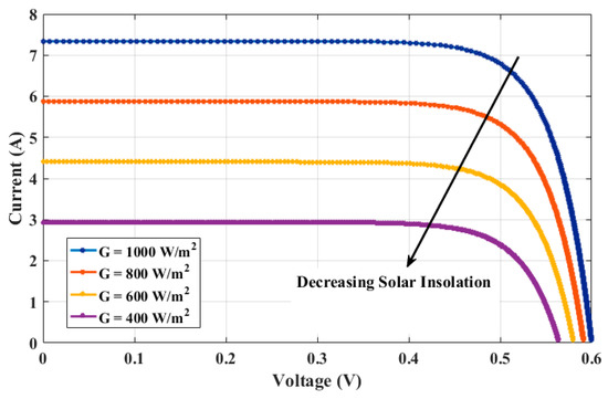
Figure 5. The stimulus of varying insolation on the I–V characteristics of the solar cell.

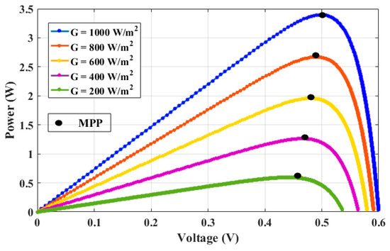
Figure 6. The impact of varying insolation on the P–V characteristics of the solar cell.

5. Partial Shading Condition

Photovoltaic systems are highly prone to partial shading. A shadow is an image cast obtained upon a surface (like a solar panel) by any obstruction intercepting the solar rays resulting in a partial shading effect (PSC). Thus, Uniform irradiance is not possible continually because of the changing environmental conditions such as rain, clouds, storms, etc. Furthermore, building shade and tree shade also contribute to shading. Hence, this effect prevents a solar panel connected in series from receiving the same incident irradiance level [8].

Due to shading on the PV array, the output power yield of the PV module decreases. The non-linearity in the PV module’s output I–V characteristics has led to multiple local maxima on the P–V curve. Thus, shading leads to hot spots that cause severe damage to these cells. Additionally, current mismatch within a PV string and voltage mismatch between parallel modules are also significant drawbacks of shadowing. The severity of the impact of shade depends on the configuration of the PV string, the type of module used, placement of the bypass diode, partial shading patterns, and the shading heaviness [9].

If partial shading of one cell occurs, then less current flows in the shaded cell in contrast with the other cells of the string. Consequently, a higher current will be forced to flow through the un-shaded cells. As a result, cells act as a diode in the reverse direction. Furthermore, the shaded cell limits the current flow in the string. Hence, the output power of the PV string decreases. Moreover, as the number of shaded cells increases, the decrease in the output power of the PV string will be more prominent.

The number of multiple peaks in the P–V curve increases with an increase in the shaded modules. Therefore, to mitigate the shading effect, a bypass diode is introduced across the string of particular cells connected in series. A bypass diode allows only unidirectional current flow. Bypass diodes, connected in anti-parallel, offer the low impedance path to power when the power flows toward the sink [10].

Under the ordinary conditions of uniform irradiance, the P–V curve presents a unique MPP, as illustrated by the curve in Figure 2. However, during partial shading, a staircase current waveform is obtained as the I–V curve. Meanwhile, the corresponding P–V curve shows the multiple peaks as depicted by Figure 7 and Figure 8, respectively.

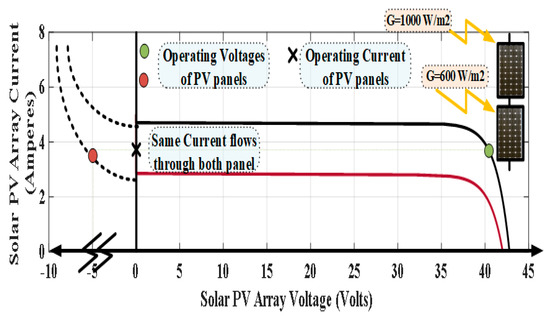
Figure 7. I–V curve under different solar insolation.

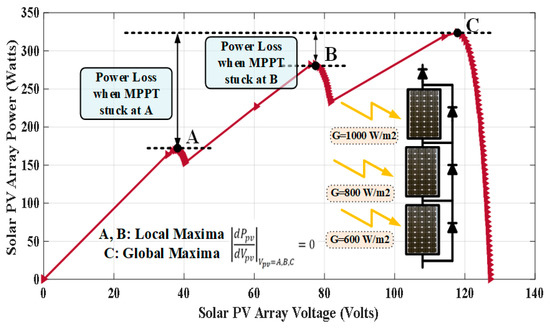
Figure 8. P–V curve at the different solar insolation.

6. Maximum Power Point Tracking Algorithms

PV array has a non-linear characteristic but has a distinct maximum power point (MPP). Therefore, to exploit the optimum power from PV panels, MPPT techniques are employed. The electronic converter enforces the MPPT algorithm. The MPPT ensures that the PV array must operate at the V_ref (reference voltage) all the time, resulting in improvements in PV panel efficiency under varying atmospheric conditions [11]. The typical block diagram of the MPPT framework is illustrated in Figure 9.

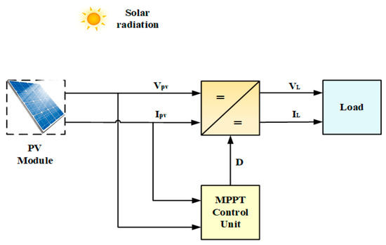
Figure 9. The typical block design of the MPPT implementation for PV systems.

6.1. Conventional MPPT Strategies

Recent developments in conventional algorithms are discussed in concise form in Table 1 at the end of this section, while in the following sub-sections, each traditional method is explained comprehensively.

6.1.1. Perturb and Observe (P&O) MPPT Technique

The P&O strategy is a broadly utilized strategy owing to its effortlessness and ease of execution [12]. Furthermore, fewer number of sensors are required, resulting in lower actualized costs [13]. The P&O MPPT algorithm deals with similar rules tothe ‘Hill Climb Search’ technique. However, the latter is less efficient than the previous one [14].

The P&O strategy is an iterative technique used to track the maximum power point (MPP). Predominantly, its operating principle works by introducing a slight disturbance in the voltage of the PV array, and the corresponding impact on the power is measured. Accordingly, the PV module voltage is elevated or decremented by varying the duty cycle of the dc–dc converter. These perturbations help in confirming whether the power is enhanced or stepped-down. Therefore, if an increment in the voltage increases the power, then the working point of the PV module is on the left edge of the P–V plot. Thus, there is a signal that the perturbation is set in a positive direction [15]. However, if an increment in the voltage prompts a decrease in the power, then the operating point is on the right edge side of the P–V plot. Hence, to follow the MPP, the perturbation direction needs to converge towards a specific end. Consequently, the iteration process is continued until the MPP is attained.

Even though the P&O strategy works well during the settled insolation, it too has few disadvantages of wavering near the MPP, a slow MPP tracking speed, and endures to locate the true MPP under partial shading conditions [13,16]. Therefore, an altered P&O technique has been proposed to conquer these drawbacks [17,18]. The standard flowchart to implement the P&O algorithm is shown in Figure 10.

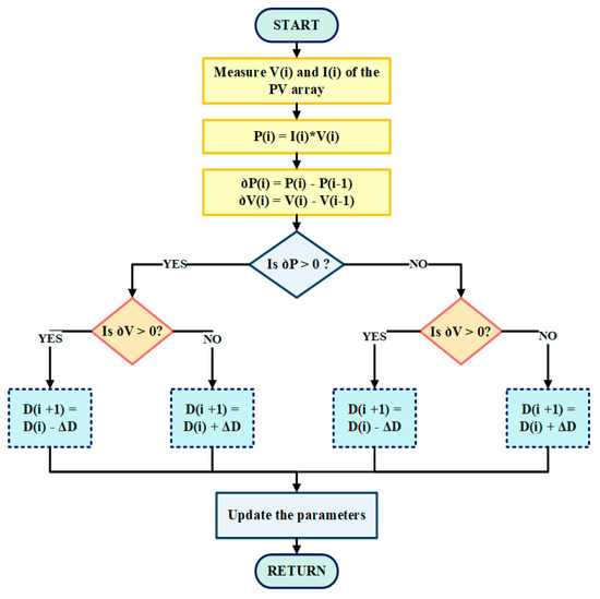
Figure 10. Flowchart to implement the P&O strategy.

6.1.2. Incremental Conductance MPPT Algorithm

The incremental conductance (INC) technique is an enhanced version of the P&O strategy. This technique is utilized in following the MPP under fast changes of atmospheric conditions [19,20].

The INC technique is principally established on the reality that the slope of power (P–V) curve of PV array is zero (∂p/∂v = 0) at MPP, positive (∂p/∂v > 0) on the left of MPP, and negative (∂p/∂v < 0) on the right of MPP.

The instantaneous power (P) is defined as the product of current and voltage.

$$P=V\times I$$

(5)

On differentiating Equation (5) with respect to V, the slope of the P–V curve can be computed as follows in Equation (6)

$$\frac{\partial P}{\partial V}=\frac{\partial \left(V\times I\right)}{\partial V}=I+V\times \left(\frac{\partial I}{\partial V}\right)$$

(6)

Therefore, the following expressions can be composed

$$\frac{\partial I}{\partial V}=-\left(\frac{I}{V}\right) \mathrm{at} \mathrm{the} \mathrm{MPP}, \mathrm{i}.\mathrm{e}., \left(\frac{\partial P}{\partial V}=0\right)$$

(7)

at the MPP, i.e., (7)

$$\frac{\partial I}{\partial V}>-\left(\frac{I}{V}\right) \mathrm{at} \mathrm{the} \mathrm{left} \mathrm{of} \mathrm{MPP}, \mathrm{i}.\mathrm{e}.,(\frac{\partial P}{\partial V}>0 )$$

(8)

at the left of MPP, i.e., (8)

$$\frac{\partial I}{\partial V}<-\left(\frac{I}{V}\right) \mathrm{at} \mathrm{the} \mathrm{right} \mathrm{of} \mathrm{MPP}, \mathrm{i}.\mathrm{e}., (\frac{\partial P}{\partial V}<0)$$

(9)

at the right of MPP, i.e., (9)

Thus, MPP can be followed by comparing incremental conductance (∂I/∂V) to an instantaneous one (I/V), as illustrated in the flowchart to implement the INC technique given in Figure 11.

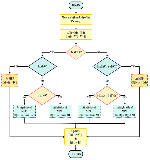
Figure 11. INC algorithm flowchart.

The INC technique can avoid oscillations in a steady state until the conditions (irradiance and temperature) are changed [21]. However, during the transition, the INC strategy acts analogous to the P&O technique. Hence, the theoretical preference of the Incremental Conductance algorithm over Perturb and Observe is lost [21,22].

6.1.3. Fractional Open Circuit Voltage MPPT Method

The Fractional Open Circuit Voltage (FOCV) MPPT technique is the least complicated indirect strategy. The FOCV method is utilized for low power functions. This algorithm can be actualized handily with digital and analog techniques. The typical block diagram of the fractional open circuit (FOCV) MPPT technique is depicted in Figure 12.

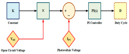
Figure 12. Fractional open circuit voltage MPPT strategy block diagram implementation.

The FOCV technique employs the theory that there exists an approximated linear relation between the maximum power point voltage (V_MPP) and open-circuit voltage (V_OC) of the PV module, as given in Equation (10).

$$V_{MPP}\approx C_V\times V_{OC}$$

(10)

where C_V signifies the proportionality constant, which depends on the PV module’s characteristics and climatic circumstances (i.e., temperature and solar insolation) [23]. C_V value varies in the range [0.71, 0.78] [24].

The FOCV technique has some drawbacks, such as the load having to be isolated during the interim, debasing the linear relationship between the V_MPP and V_OC with time, and additional types of equipment are needed to measure V_OC after a specific interval [25].

6.1.4. Fractional Short Circuit Current Technique

The Fractional Short Circuit Current (FSCC) technique is additionally an indirect technique practically identical to the FOCV method. The FSCC technique is actualized on the fact that there exists a straight-line relationship between the current at the maximum power point (I_MPP) and the short circuit current (I_SC) of the PV module, as demonstrated in Equation (11) [26]. The block diagram of the FSCC strategy is represented in Figure 13.

$$I_{MPP}\approx C_I\times I_{SC}$$

(11)

where C_I denotes the invariable current factor which generally varies between [0.78, 0.92] [27].

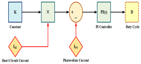
Figure 13. Fractional short-circuit current MPPT strategy schematic diagram.

During the short circuit condition, V_out is zero, resulting in zero output power. Hence, it is a squander of energy.

Table 1. Recent research work done in the field of conventional MPPT strategies.

Authors, Year	Strategies Involved	Control Parameter	DC-DC Converter	Controller Implementation	Findings/Remarks
M. H. Osman, et al. [28], 2021	Traditional, two-step size, and variable-step scale P&O	V	Boost converter	MATLAB/Simulink	A trade-off between steady-state and dynamic performance can be easily handled by the variable-step and two-step strategies. Improved stability in case of external atmospheric changes (i.e., temperature and irradiation). Modified algorithms track the MPP in half of the time taken by traditional P&O.
G. A. Raiker, et al. [29], 2021	Momentum-based P&O + voltage directed current control	V and I	Boost Converter	TMS320F28379D, C2000 series controller	The utilization of current control causes a fast response to rapid variations in irradiation. Momentum-based P&O enhances the tracking rate by enlarging the step size of the P&O MPPT while preserving the oscillation magnitude. Change to traditional P&O is simply carried out by employing a storage variable. Oscillations attenuated by 30% and following speed incremented by a factor of two.
S. Manna, et al. [30], 2021	Conventional, drift-free, and updated, P&O MPPT methods.	Du	Boost converter	MATLAB/Simulink	In terms of efficiency and tracking power, the drift-free technique presents better results in contrast with the other two strategies. Power loss decreases as the drift-free P&O method can trace several radiation profiles accurately with a small perturbation from the MPP.
P. E. Sarika, et al. [31], 2020	Variable Step Size Zero Oscillation P&O (i.e., VSS ZOPO)+ Look-Up Table (LUT) technique	Du	Boost converter	MATLAB/Simulink	VPV and IPV serve as breakpoint data for the LUT strategy. Hence, there is no need for skilled knowledge and trained data in implementing the VSS ZOPO-LUT algorithm. The strategy responds quickly. Thus, the method demonstrates less tracking time. The proposed algorithm exhibits almost zero oscillations around MPP.
D. Ounnas, et al. [32], 2021	Modified INC strategy	Step size and permitted error	Boost converter	MATLAB/Simulink, and Arduino mega board	To overcome the problem of choosing step size, the notion of variable step size is introduced. Right decision judgment is verified by utilizing permitted error during a sudden change in solar insolation level. Fast convergence to reach the MPP with fewer oscillations.
M. Hebchi, et al. [33], 2021	Improved INC algorithm	$\frac{I}{V}$&$\frac{∆I}{∆V}$	Boost converter	MATLAB/Simulink	The likelihood to change the preliminary constraint during the search procedure is a significant benefit of this method. This method successfully improves the search dynamics of the pulse position modulation. Hence, the proposed strategy gives a practical solution, notably for provinces with repetitive solar irradiance and high insolation change. An insightful approach is needed to select the fair values for the ideal working of the proposed method.
M. A. B. Siddique, et al. [34], 2021	Linearly modified INC-MPPT method	$\frac{∆I}{∆t}$&$\frac{∆V}{∆t}$	Boost converter	MATLAB/Simulink	The proposed technique conveys zero oscillation in the yield power of the solar photovoltaics system during MPP tracking. Accurate and efficient MPP tracking of the PV system. More reliable MPPT strategy.
M. N. Ali, et al. [35], 2021	Variable step INC + FLC MPPT method	Du	Boost converter	MATLAB/Simulink	FLC block is utilized for changing the step size of the voltage of the INC MPPT strategy per the fuzzy inputs. Duty cycle adjusts the VPV by the variable step INC method. The suggested algorithm improves the PPV and decreases the convergence time during changing climatic conditions.
D. Baimel, et al. [36], 2019	Semi-pilot cell (SPC) FOCV and Semi-pilot panel (SPP) FOCV strategy	VOC	Buck-Boost converter	MATLAB/Simulink	Replacement of pilot cell by SPC aids in power loss reduction during measurement of open-circuit voltage. SPP FOCV and SPC FOCV MPPT algorithms can accurately assess the VMPP. Hence, the overall efficiency of the PV system is enhanced. SPP-FOCV is not intended to be implemented during PSCs.
M. Krishnan M, et al. [37], 2019	FOCV + P&O MPPT algorithms	VOC	Buck converter	MATLAB/Simulink	Rapid MPP tracking. Reduction in perturbation magnitude during P&O tracking mode improves the PV system’s efficiency and lessens the oscillation around MPP without affecting the tracking speed. No need for an external sensor to sense Voc during varying climatic conditions.
K. R. Bharath, et al. [38], 2017	Improved FOCV technique	Experimentally calculated factor; k	Buck Converter	AVR supported ATMega16 microcontroller	Periodic open-circuit voltage check improves the algorithm’s efficiency by briefly impeding the energy drawn from the PV panel and supporting a vital switching sequence to the converter. Effective when temperature change leads to variation in VOC. A single sensor is employed to sense voltage and load.
C. B. N. Fapi, et al. [39], 2021	Enhanced FSCC MPPT strategy	$\frac{I_{PV}}{I_{SC}}$	Boost Converter	Matlab/Simulink + Control Desk Software + DS1104 control board	Direct detection of the ISC by basically reading the IPV through decrement and increment in solar irradiance. During changing atmospheric conditions, the proposed algorithm shows a short following time and increases power production.
H. A. Sher, et al. [40], 2015	Modified FSCC MPPT technique	$\frac{I_{PV}}{I_{SC}}$ error	Buck-Boost converter	Matlab/Simulink + dSPACE DS1104 based controller board	The strategy consists of two loops: standard loop and IPV loop. The suggested algorithm eliminates the need of the irradiance sensor. Cost-effective alternative for low price solar PV appliance without compromising on the energy loss.

Note: Du—Duty cycle, V_OC—Open circuit voltage, I_PV—PV array current, I_SC—Short circuit current.

Table 1. Recent research work done in the field of conventional MPPT strategies.

Authors, Year	Strategies Involved	Control Parameter	DC-DC Converter	Controller Implementation	Findings/Remarks
M. H. Osman, et al. [28], 2021	Traditional, two-step size, and variable-step scale P&O	V	Boost converter	MATLAB/Simulink	A trade-off between steady-state and dynamic performance can be easily handled by the variable-step and two-step strategies. Improved stability in case of external atmospheric changes (i.e., temperature and irradiation). Modified algorithms track the MPP in half of the time taken by traditional P&O.
G. A. Raiker, et al. [29], 2021	Momentum-based P&O + voltage directed current control	V and I	Boost Converter	TMS320F28379D, C2000 series controller	The utilization of current control causes a fast response to rapid variations in irradiation. Momentum-based P&O enhances the tracking rate by enlarging the step size of the P&O MPPT while preserving the oscillation magnitude. Change to traditional P&O is simply carried out by employing a storage variable. Oscillations attenuated by 30% and following speed incremented by a factor of two.
S. Manna, et al. [30], 2021	Conventional, drift-free, and updated, P&O MPPT methods.	Du	Boost converter	MATLAB/Simulink	In terms of efficiency and tracking power, the drift-free technique presents better results in contrast with the other two strategies. Power loss decreases as the drift-free P&O method can trace several radiation profiles accurately with a small perturbation from the MPP.
P. E. Sarika, et al. [31], 2020	Variable Step Size Zero Oscillation P&O (i.e., VSS ZOPO)+ Look-Up Table (LUT) technique	Du	Boost converter	MATLAB/Simulink	VPV and IPV serve as breakpoint data for the LUT strategy. Hence, there is no need for skilled knowledge and trained data in implementing the VSS ZOPO-LUT algorithm. The strategy responds quickly. Thus, the method demonstrates less tracking time. The proposed algorithm exhibits almost zero oscillations around MPP.
D. Ounnas, et al. [32], 2021	Modified INC strategy	Step size and permitted error	Boost converter	MATLAB/Simulink, and Arduino mega board	To overcome the problem of choosing step size, the notion of variable step size is introduced. Right decision judgment is verified by utilizing permitted error during a sudden change in solar insolation level. Fast convergence to reach the MPP with fewer oscillations.
M. Hebchi, et al. [33], 2021	Improved INC algorithm	$\frac{I}{V}$&$\frac{∆I}{∆V}$	Boost converter	MATLAB/Simulink	The likelihood to change the preliminary constraint during the search procedure is a significant benefit of this method. This method successfully improves the search dynamics of the pulse position modulation. Hence, the proposed strategy gives a practical solution, notably for provinces with repetitive solar irradiance and high insolation change. An insightful approach is needed to select the fair values for the ideal working of the proposed method.
M. A. B. Siddique, et al. [34], 2021	Linearly modified INC-MPPT method	$\frac{∆I}{∆t}$&$\frac{∆V}{∆t}$	Boost converter	MATLAB/Simulink	The proposed technique conveys zero oscillation in the yield power of the solar photovoltaics system during MPP tracking. Accurate and efficient MPP tracking of the PV system. More reliable MPPT strategy.
M. N. Ali, et al. [35], 2021	Variable step INC + FLC MPPT method	Du	Boost converter	MATLAB/Simulink	FLC block is utilized for changing the step size of the voltage of the INC MPPT strategy per the fuzzy inputs. Duty cycle adjusts the VPV by the variable step INC method. The suggested algorithm improves the PPV and decreases the convergence time during changing climatic conditions.
D. Baimel, et al. [36], 2019	Semi-pilot cell (SPC) FOCV and Semi-pilot panel (SPP) FOCV strategy	VOC	Buck-Boost converter	MATLAB/Simulink	Replacement of pilot cell by SPC aids in power loss reduction during measurement of open-circuit voltage. SPP FOCV and SPC FOCV MPPT algorithms can accurately assess the VMPP. Hence, the overall efficiency of the PV system is enhanced. SPP-FOCV is not intended to be implemented during PSCs.
M. Krishnan M, et al. [37], 2019	FOCV + P&O MPPT algorithms	VOC	Buck converter	MATLAB/Simulink	Rapid MPP tracking. Reduction in perturbation magnitude during P&O tracking mode improves the PV system’s efficiency and lessens the oscillation around MPP without affecting the tracking speed. No need for an external sensor to sense Voc during varying climatic conditions.
K. R. Bharath, et al. [38], 2017	Improved FOCV technique	Experimentally calculated factor; k	Buck Converter	AVR supported ATMega16 microcontroller	Periodic open-circuit voltage check improves the algorithm’s efficiency by briefly impeding the energy drawn from the PV panel and supporting a vital switching sequence to the converter. Effective when temperature change leads to variation in VOC. A single sensor is employed to sense voltage and load.
C. B. N. Fapi, et al. [39], 2021	Enhanced FSCC MPPT strategy	$\frac{I_{PV}}{I_{SC}}$	Boost Converter	Matlab/Simulink + Control Desk Software + DS1104 control board	Direct detection of the ISC by basically reading the IPV through decrement and increment in solar irradiance. During changing atmospheric conditions, the proposed algorithm shows a short following time and increases power production.
H. A. Sher, et al. [40], 2015	Modified FSCC MPPT technique	$\frac{I_{PV}}{I_{SC}}$ error	Buck-Boost converter	Matlab/Simulink + dSPACE DS1104 based controller board	The strategy consists of two loops: standard loop and IPV loop. The suggested algorithm eliminates the need of the irradiance sensor. Cost-effective alternative for low price solar PV appliance without compromising on the energy loss.

Note: Du—Duty cycle, V_OC—Open circuit voltage, I_PV—PV array current, I_SC—Short circuit current.

6.2. Meta-Heuristic Techniques

The classification of the meta-heuristic algorithm reviewed in this article is illustrated in Figure 14.

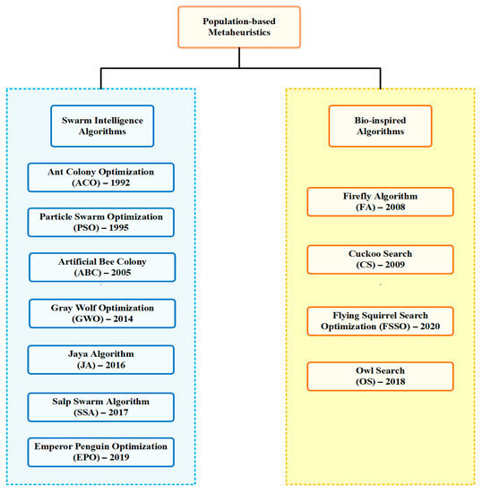
Figure 14. Categorization of reviewed meta-heuristic strategies.

6.2.1. Swarm Intelligence Methods

This section sub-part explains each swarm intelligence technique in a detailed manner. Additionally, at last, current work related to these algorithms is tabulated in Table 2.

(a) 

Particle Swarm Optimization Method

The Particle Swarm Optimization (PSO) technique is among the most widely used random search methods. The PSO strategy maximizes the nonlinear continuous functions. The PSO strategy was suggested by Eberhart and Kennedy in 1995 [41].

The functioning rule of the PSO algorithm is demonstrated after the natural demeanor of fish schooling and flock gathering [42]. In this strategy, numerous collaborative birds are employed, and each bird signifies a particle.

Each particle has its fitness value in the search space, which is mapped by a position vector and velocity vector. Furthermore, each particle utilizes its fitness value to choose the direction and distance of its step. After that, each particle proposed a resolution by trading the information obtained in its particular search process to find the best solution. The primary flowchart of PSO methodology is depicted in Figure 15.

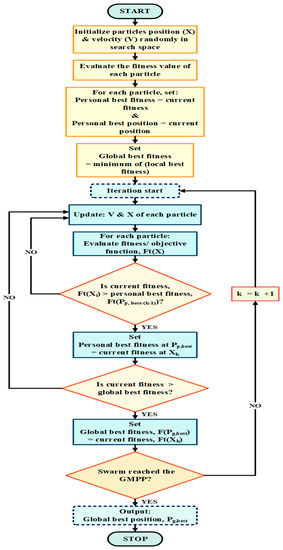
Figure 15. Typical PSO MPPT technique flowchart.

The PSO method initializes with a group of random solutions (position and velocity for each particle) in the search arena. After each iteration, particles change their fitness value by employing an intellectual, social trade-off. The trade-off leads to a change in the individual best (P_p,best) and neighborhood’s (characterized as the entire populace or as the subset of it) best position (P_g,best).

Every particle remembers the individual best of all particles in addition to the global best position. Thus, the swarm attempts to find the best solution by refreshing the position and velocity after every cycle. Subsequently, each particle rapidly converges to the global maxima. The refreshing conditions [43] for the position (X) and velocity (V) of the nth molecule for the kth cycle are given in Equations (12) and (13).

$$V_n\left(k+1\right)=\omega V_n\left(k\right)+s_1{\rho }_1\left(P_{p, best-k}-X_n\left(k\right)\right)+s_2{\rho }_2\left(P_{g, best}-X_n\left(k\right)\right)$$

(12)

$$X_n\left(k+1\right)=X_n\left(k\right)+V_n\left(k+1\right)$$

(13)

n = 1, 2, 3, …, N

where k signifies the iteration count; X_n corresponds to the position of the nth particle; $V_n$ indicates the velocity of the nth particle; ω represents the inertia burden; s₁, s₂ denote the social and cognitive acceleration coefficients, respectively; ${\rho }_1$, ${\rho }_2$ indicate the arbitrary variables and their assessments are uniformly distributed between zero and one; P_p,best-i signifies the individual optimal position of the nth particle at the kth iteration; P_g,best implies the swarm–optimum position. If an extempore situation, such as the condition in Equation (14) of initialization, was satisfied, then the method update is in accordance with Equation (15).

Ft(X_n−k) > Ft(P_p,best-k)

(14)

P_p,best-k = X_n-k

(15)

where Ft shows the target function needed to be maximized.

Although the traditional PSO strategy can track the global maximum power point GMPP under all cases, its overall tracking speed is slower than the common INC method for certain cases [44]. Various variations of the PSO procedure can be procured by consolidating it with other developmental techniques. There is a pattern in exploration to make a cross variety of the PSO algorithm to improve the general advancement of the computation. Some used variations of the PSO estimation are introduced in [44,45,46].

Applications: PSO strategy discovered its first application in the field of neural network training. From that point forward, it has been utilized in a wide assortment of fields like power systems, telecommunications, configuration, power frameworks, control, and numerous others. A PSO algorithm has been employed in the following cases, such as the Min–Max issues and different advancement problems.

(b) 

Ant Colony Optimization Strategy

The Ant Colony Optimization (ACO) strategy is the ant systems’ most distinguished and effective substitution. Macro Dorigo first proposed the ant system in 1992 [47]. Later, further enhancements were done by Gambardella in1997 to ant systems [48].

The ACO technique is inspired by the cooperative searching conduct of ants searching for the shortest route between their colony and source food. The trail-laying and trail-following conduct of ants is the foundation of the ACO strategy. The flowchart of the ACO algorithm is depicted in Figure 16.

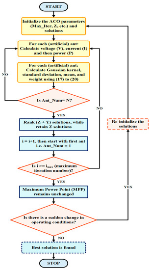
Figure 16. Flowchart of the ACO strategy.

At first, ants wander in random directions. When one or more ants come across the food source, they re-visit their province (with food), while leaving behind pheromone trails. Ants use pheromone as a means of communication. The pheromone consists of specific synthetic substances delivered by living beings to impart messages or signs to different individuals of a similar species. If other ants discover such a path, they follow the route to the food source contrary to meandering arbitrarily. When they re-visit their province, they also leave pheromones, resulting in enriching the current pheromone intensity. Pheromone evaporates with time, in this way reducing the strength of the pheromone. Eventually, the ants adjust and locate the briefest course to the food source.

The process begins by considering a single colony of (artificial) ants placed arbitrarily in that colony. Let there be N parameters indicating ants. Each ant in the population entices another ant with its magnetic force. Contingent upon the attractive force, the ants relocate from the lower strength zone to the higher strength zone. After every iteration cycle, the appealing power is determined. As per the results, ants move towards the optimum solution.

At first, consider an issue where N parameters (artificial ants) are to be optimized such that Z ≥ N. Z symbolizes the initially generated random solutions and is stored in the solution chronicle. Then the result is positioned as per their fitness value Ft(s_i), as demonstrated in Equation (16).

$$\mathrm{Ft}\left({\mathrm{s}}_1\right) \le \mathrm{Ft}\left({\mathrm{s}}_2\right) \le \mathrm{Ft}\left({\mathrm{s}}_3\right) \dots \le \mathrm{Ft}\left({\mathrm{s}}_{\mathrm{N}}\right)$$

(16)

Likewise, new arrangements are formed by sampling the Gaussian Kernel function to ascertain the ants’ positions by following Equation (17).

$${\mathsf{Ĝ}}_i\left(x\right)={\displaystyle \sum }_{k=1}^z{ŵ}_k{\hat{g}}_k^i\left(x\right)={\displaystyle \sum }_{k=1}^z{w}_k\frac{1}{{\stackrel{\sim }{\sigma }}_k^i\sqrt{2\pi }}{e}^{\left[-\frac{{\left(x-{\hat{\mu }}_k^i\right)}^2}{2{\left({\tilde{\sigma }}_k^i\right)}^2}\right]}$$

(17)

where Ĝ_i(x) denotes the Gaussian kernel for the ith dimension of the solution;

• $ŵ$_k indicates the weight factor for the kth solution;
• ${ĝ}_k^i$ represents the kth sub-Gaussian function for the ith dimension;
• ${\tilde{\sigma }}_i^k$ symbolizes the ith dimensional standard deviation for the kth solution;
• ${\hat{\mu }}_k^i$ signifies the ith means value for the kth solution.

Utilizing Z initial solutions, the computation for the standard deviation, mean value, and weight factor can be done following Equations (18)–(20), respectively.

Standard Deviation:

$${\tilde{\sigma }}_k^i=\in {\displaystyle \sum }_{k=1}^z\frac{\left|s_k^i-s_k^i\right|}{Z-1}$$

(18)

where $\in$ symbolizes the convergence rate.

Mean Value:

$${\hat{\mu }}^i=\left\{{\hat{\mu }}_1^i,\dots , {\hat{\mu }}_k^i,\dots ,{\hat{\mu }}_z^i\right\}=\left\{s_1^i,\dots ,s_k^i,\dots ,s_z^i\right\}$$

(19)

Weight:

$${ŵ}_k=\frac{1}{\phi Z\sqrt{2\pi }}{e}^{\left[-\frac{{\left(k-1\right)}^2}{2{\left(\phi Z\right)}^2}\right]}$$

(20)

where φ represents the best optimal operating solution.

The probability value of selecting the kth Gaussian function can be evaluated using Equation (21).

$$P_k=\frac{{ŵ}_k}{{{\displaystyle \sum }}_{j=1}^z{ŵ}_j}$$

(21)

The examining cycle will be continued as per the number of parameters to be enhanced. Create Y new solutions that sum up to the Z initial solutions. Then, the Z + Y solutions need to be positioned in the search area. Later, Z’s best arrangements are re-established once more. In this way, the whole cycle is re-hashed for the necessary number of iterations [49].

The ACO method effectively tracks the global MPP dissimilar to the traditional optimization techniques. The ACO algorithm has a higher convergence rate. In addition, ACO requires a lesser number of iterations to get the result. Hence, the ACO method is more advantageous compared to other algorithms.

Applications: The ACO method is naturally appropriate for discrete value optimization problems [50]. Furthermore, ACO can handle continuous value optimization. However, the design vector in the continuous value problem ought to be transformed into little discrete advances. Moreover, ACO discusses earlier works with input–output mapping only like all other algorithms. Therefore, subsidiary data of objective work is not fundamental.

(c) 

Artificial Bee Colony Technique

The Artificial Bee Colony (ABC) method is centered on the honey bees’ intelligent foraging conduct. The ABC algorithm was proposed by Dervis Karaboga in 2005 to improve the polynomial mathematical issues [51]. The ABC strategy is sensibly a modern stochastic algorithm for global optimization. The fundamental flowchart of the ABC strategy is depicted in Figure 17.

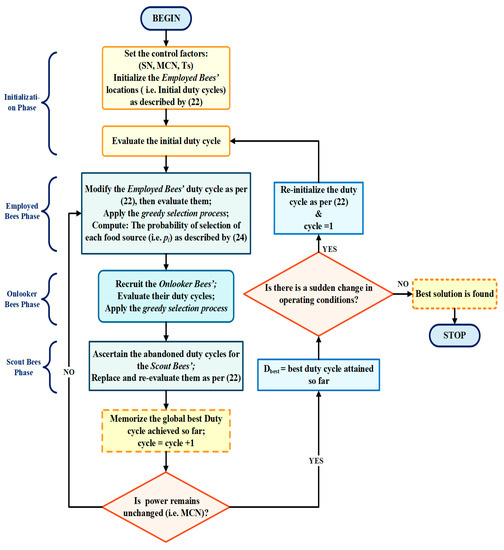
Figure 17. Flowchart of the ABC technique.

The honey bees live within the frame of the province (i.e., in the hives). The honey bees can communicate with one another utilizing pheromone (chemical trade) and the waggle dance. If any bee discovers the nourishment source, and it brings back some food to the province, it trades off the food source location through a waggle dance. The strength and span of the waggle dance demonstrate the extravagance of the food source found. The waggling moves change from one group of species to another group.

The ABC strategy divides the artificial bees into the following three classes: employed bees, onlooker bees, and scouts. Half of the honey bee province consists of employed bees and another half of the onlooker bees. The objective of the entire ant group is to locate the optimum source of nectar, signifying the food. Initially, employed honey bees search for a food source, return to the hive and share their data through the waggle dance moves. The onlooker honey bees attempt to discover a food source by watching the employed honey bee’s waggle dance, whereas scout honey bees look for new food sources haphazardly. The communication of honey bees is subject to the quality of the food source. The likelihood of sharing the data by employed bees is straightforwardly relative to the productivity of food sources. In this way, artificial honey bees communicate and coordinate among themselves to obtain optimal solutions in a brief time [52,53].

To simplify the ABC solution process, mathematically and logically, the following assumptions have to be considered [54]:

• In the solution course, the sources reached by the bees in the food search relate to the possible optimum values. In the ABC strategy, the nectar amount is computed. The nectar idea is utilized in light of the nature of the solution values gainedfrom the sources.
• The nectar (food) in each source must be taken by only one employer bee. For this situation, the absolute number of food sources and employer bees are considered equivalent.

The ABC algorithm employed the following steps to track the GMPP:

• Step-1 [Initialization Phase]: Randomly build N_s food source in the search space. The larger the group is, the better is the performance of the algorithm. To distribute all the employed bees corresponding to each unique food source as per Equation (22), each solution X_i is an n-dimensional vector.

$$X_{i,j}=X_{min,i}+rand\left[0,1\right]\left(X_{max,i}-X_{min,i}\right)$$

(22)

$$i=1, 2, 3,\dots , N_s; j=1, 2, 3,\dots , n$$

where n specifies the number of optimization parameters; X_max,i and X_min,i indicate the maximum and the minimum value of the nth dimension, respectively.

• Step-2 (Employed Bee Phase): The aim is to follow the food source position with maximum nectar available (i.e., GMPP) in the search area. Each employed bee advances its new position (V_i,j) in the proximity space using the old position value (X_i) to keep safely in memory, as per Equation (23).

$$V_{i,j}=X_{i,j}+{\alpha }_{i,j}\left(X_{i,j}-X_{k,j}\right); k=1, 2,3, \dots N_s$$

(23)

where X_k indicates the randomly selected food source other than X_i, i.e., k should be different from ‘i’; α_i,j indicates the random number between them [−1, 1].

When the employed honey bee investigates another food source location, it uses the greedy selection strategy. This strategy involves a comparison of the amount of nectar present at the old and new positions. Thus, it preserves a better solution.

• Step-3 (Onlooker Bee Phase): According to the information (i.e., the nectars in the food sources) conveyed by the employed bees to the onlooker bees with the assistance of a waggle dance, onlooker bees perform the probabilistic selection process for the selection of food sources (solutions). The probability of selection of each food source is computed using Equation (24).

$${\hat{p}}_i=\frac{f\left(x_i\right)}{{{\displaystyle \sum }}_{n=1}^{N_s}f\left(x_i\right)}; i=1, 2, 3,\dots , N_s$$

(24)

where f(x) represents the fitness factor as per the food resource.

• Step-4 (Scout Bee Phase): As per Equation (24), scout bees can discover new promising solutions around the selected food source. In any case, the fitness value of a food source remains unenhanced for the given step even after the inspection of the whole search area by employed and onlooker bees. In the next step, the corresponding employed bees become scout bees, and the scout bees look for new possible solutions, utilizing Equation (22).
• Step-5 (Conclusion Phase): The entire procedure ceases when there is no further improvement in the output power. However, when there is a fluctuation in the output power, the process will reinitiate. The fluctuation effect can be because of solar insolation changes. Such changes in insolation are represented by the inequality condition, represented in Equation (25).

$$\left|\frac{P_{pv}-P_{pv, old}}{P_{pv, old}}\right|\ge ∆P_{pv}\%$$

(25)

The GMPP search will again start if the above-mentioned criterion in (25) is satisfied. Hence, the ABC strategy can indeed distinguish the genuine MPP regardless of partial shading conditions.

(d) 

Grey Wolf Optimization Technique

The Grey Wolf Optimization (GWO) technique was advised by Mirjalili et al. in the year 2014. The GWO strategy is inspired by grey wolves’ social hierarchy and hunting conduct in nature [55]. Generally, grey wolves prefer to live in a pack. The average grey wolf pack size is in the [5,12] range. Based on the social dominance attribute, the grey wolves are categorized into four types, as per the hierarchical sequence shown in Figure 18. At the top, Alpha (ά) wolves are the pioneers and are hence considered to be the fittest solution for a given optimization issue. Beta (β′) wolves come after ά wolves’ and help the ά wolves in obligations. Therefore, β′ wolves can substitute ά wolves if they die. The second last category consists of the delta (δ′) wolves, which constitute the hunters, keepers, and explorers of the pack. Hence, β′ and δ′ wolves stand for the second and third-best solutions, respectively. The last category is Omega (ώ) wolves. Ώ wolves are the young members of the pack, and hence represent the remaining solutions [56]. The dominance of wolves decreases in correspondence to the decrease in the rank of wolves from the top to the bottom in a hierarchical sequence. The primary flowchart of the GWO strategy is depicted in Figure 19.

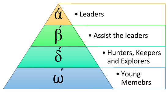
Figure 18. The hierarchical sequence of grey wolves.

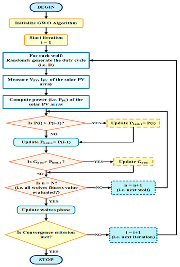
Figure 19. Flowchart of the GWO MPPT algorithm.

Other than the social order of wolves, aggregate hunting also significantly involves the social conduct of grey wolves. Based on this, the mathematical model of the GWO algorithm considers the following measure [56]: social hierarchy, tracking and encircling, hunting, searching, and attacking the prey as follows:

• Social Hierarchy:

To model the hierarchical system of wolves in the GWO technique, assume the fittest solution as the alpha (ά) followed by beta (β′) and delta (δ′) as the second and third best solutions, respectively. The remaining candidate solutions are supposed to be omega (ώ). In this way, the hunting process is guided by alpha, beta, and delta wolves, while the omega wolves follow them.

ii.

Tracking and Encircling the prey:

During the hunting process, grey wolves usually encircle prey. The mathematical functions stated in Equations (26) and (27) indicate the encircling process. Equation (26) estimates the distance vector $\overrightarrow{Ḑ}$ of a wolf from prey.

$$\overrightarrow{Ḑ}=\left|\overrightarrow{Ḅ.}\overrightarrow{{Ẋ}_{P_{Gw}}}\left(i\right)-\overrightarrow{{Ẋ}_P}\left(i\right)\right|$$

(26)

$$\overrightarrow{{Ẋ}_P}\left(i+1\right)=\overrightarrow{{Ẋ}_{P_{GW}}}\left(i\right)-\overrightarrow{Ạ}.\overrightarrow{Ḑ}$$

(27)

where ‘i’ indicates the current iteration; $\overrightarrow{{Ẋ}_P}$ signifies the prey vector; $\overrightarrow{{Ẋ}_{P_{GW}}}$ denotes the grey wolf (GW) position vector; $\overrightarrow{Ạ}, \overrightarrow{Ḅ}$ are the coefficient vectors computed utilizing Equations (28) and (29), respectively.

$$\overrightarrow{Ạ}=2\overrightarrow{\mathsf{á}}.\overrightarrow{{\mathsf{ŕ}}_1}-\overrightarrow{\mathsf{á}}$$

(28)

$$\overrightarrow{Ḅ}=2\overrightarrow{{\mathsf{ŕ}}_2}$$

(29)

where $\overrightarrow{{\mathsf{ŕ}}_1}, \overrightarrow{{\mathsf{ŕ}}_2}$ stand for the arbitrary variables in the range [0, 1], and during each iteration, ‘á’ linearly decreases from 2 to 0.

iii.

Hunting:

Based on the random vectors ($\overrightarrow{{\mathsf{ŕ}}_1}$ and $\overrightarrow{{\mathsf{ŕ}}_2)}$, a wolf can reach any position between the points.

Initially, the first three finest solutions (i.e., the location of alpha, beta, and delta wolves) are stored. As per the best solution knowledge, other searching wolves update their position. Therefore, a grey wolf can upgrade its location in any random direction by employing (30).

$$\overrightarrow{{Ḑ}_{\alpha }}=\left|\overrightarrow{{Ḅ}_1}. \overrightarrow{{Ẋ}_{\alpha }}-\overrightarrow{Ẋ}\right|$$

$$\overrightarrow{{Ḑ}_{\delta }}=\left|\overrightarrow{{Ḅ}_3}. \overrightarrow{{Ẋ}_{\delta }}-\overrightarrow{Ẋ}\right|$$

$$\overrightarrow{{Ẋ}_1}=\overrightarrow{{Ẋ}_{\alpha }}-\overrightarrow{{Ạ}_1}.\overrightarrow{{Ḑ}_{\alpha }}$$

$$\overrightarrow{{Ẋ}_2}=\overrightarrow{{Ẋ}_{\beta }}-\overrightarrow{{Ạ}_2}.\overrightarrow{{Ḑ}_{\beta }}$$

$$\overrightarrow{{Ẋ}_3}=\overrightarrow{{Ẋ}_{\delta }}-\overrightarrow{{Ạ}_3}.\overrightarrow{{Ḑ}_{\delta }}$$

$$\overrightarrow{Ẋ}\left(i+1\right)=\frac{\overrightarrow{{Ẋ}_1}+\overrightarrow{{Ẋ}_2}+\overrightarrow{{Ẋ}_3}}{3}$$

(30)

iv.

Attack the prey:

As the ‘á’ linearly decreases from 2 to 0 in each cycle. Therefore, when the $\left|Ạ\right|<1$ condition is satisfied, the prey halts at a fixed position, following which the grey wolves attack the prey.

v.

Search for a prey:

When the $\left|\mathsf{Ạ}\right|>1$ condition is reached, grey wolves are forced to search the target. This process depicts the exploration method, where the wolves move away from each other in search of prey, and later move towards each other to attack the prey.

The implementation of the GWO strategy for MPPT tracking starts by assuming the initial positions of wolves (Ẋ) and the best location (P_best) of them [57]. In this optimization process, ‘i’ iterations are employed to determine the best position of the wolf. Hence, in the ith iteration, there will be ith iteration values for the position of N wolf pack, i.e., Ẋ_1,i, Ẋ_2,i, …, Ẋ_k,i, …, Ẋ_N,i. Therefore, this technique focuses on determining the next iteration value of the location for wolves (particles). In this way, the wolves get closer to their objective, i.e., the maximum power.

(e) 

Emperor Penguin Optimization MPPT Technique

Emperor penguins gather during the Antarctic winter for their survival. Thousands of emperor penguins gather in huge colonies during breeding and spend their lives in open ice throughout the winter season. The emperor penguins have neighbors who are selected arbitrarily in the herd [58]. The EPO is motivated by the social gathering conduct of emperor penguins. They position themselves on a polygon-shaped grid periphery during the gathering. The wind that flows around the huddle is determined to find the huddle border line around a polygon. Since emperor penguins’ habitat is on the Antarctic continent, the low temperature throughout the winter makes their survival difficult. They flock in a huddle to maintain their body temperature at an appropriate limit necessary for their survival. Gathering behavior is shown by emperor penguins only. It depends on many attributes, for example, distance, temperature, and efficacious penguins throughout the herd. Maximizing the ambient temperature in the huddle is the crucial motive of the emperor penguins’ gathering [59]. The basic flowchart of the GWO algorithm is exhibited in Figure 20.

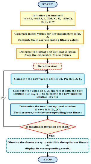
Figure 20. Flowchart to implement the EPO strategy.

The following steps describe the huddling conduct of emperor penguins:

• Identify and set the huddle boundary of emperor penguins’;
• Measurementof the temperature profile of the herd;
• Calculationof the distance between emperor penguins. The distance is responsible forexploration and exploitation;
• The effective mover (the best optimal solution) is procured;
• Reposition of the effective mover.

A temperature profile with different locations guides exploration and exploitation for emperor penguins. Temperature (TM) relies on the radius of the herd polygon p as follows:

$$TM=\left\{\begin{array}{l} 0;p>1\\ 1;p<1\end{array}\right.$$

(31)

Moreover, TM₀, a temperature parameter, identifies the exploration and the exploitation as stated in Equation (32).

$$T{M}_0=TM-\frac{MX}{PX-MX}$$

(32)

where TM₀ indicates the temperature profile of the herd; MX symbolizes the maximum total count of iterations; PX denotes the present iteration.

Subsequently, for the herd boundary identification, the distance between the emperor penguins and the best optimal solution d is calculated as follows:

$$d=SF\left(C\right)B_{ep}\left(x\right)-E\times B\left(x\right)$$

(33)

where SF(C) describes the social forces of emperor penguins; B(x) represents the recent position vector of the emperor penguin; C and E are anti-collision factors between neighbors; B_ep(x) corresponds to the vector of the best optimal solutions discovered.

C and E are accountable for tuning the distance (d) and can be computed using Equations (34) and (35).

$$E=\mathrm{rand} 2$$

(34)

$$C=m\left(T{M}_0+\mathrm{PG}\left(\mathrm{te}\right)\right)\times \mathrm{rand} 3-T{M}_0$$

(35)

where m stands for the movement parameter that upholds a gap between search agents for collision evasion whose estimation is taken as 2; PG(te) indicates the polygon grid accuracy by evaluating the difference between emperor penguins; rand2 belongs to (0, 1) and rand 3 lies in the interval (0, 1). SF(C) directs the way towards the best optimal hunt agent, computed using Equation (36), and the position is updated by utilizing Equation (37).

$$SF\left(C\right)={(\sqrt{T{e}^{-\raisebox{1ex}{$x$}\!\left/ \!\raisebox{-1ex}{$w-$}\right.}}{e}^{-x})}^2$$

(36)

$$B\left(x+1\right)=B_{ep}\left(x\right)-C\times d$$

(37)

where T and w indicate the restrain parameters for better exploration and exploitation. T lies between (2 and 3), and w varies from 1.5 to 2; B(x + 1) signifies the n following the modified location of the emperor penguin.

The steps involved in EPO execution are as follows:

• Step 1: Initialize rand2, rand3, p, TM, $T{M}_0$, C, E, SF(C), m, T, and w.
• Step 2: Develop initial values for essential parameters like B(x). Then, estimate theirequivalentfitness values.
• Step 3: Set the initial best optimal solution among the initially calculated fitness values.
• Step 4: Begin the first iteration by computing the new values of TM₀, SF(C), PG(te), and C.
• Step 5: Compute the value of d. Then, operate it in the best solution; B_ep(x) function toevaluate the newly updated solution B(x + 1).
• Step 6: Evaluate the new best optimal solution and save it in B_ep(x). Furthermore, save the corresponding best fitness.
• Step 7: Check for maximum iteration count if it has not been reached. Then, replicate until the maximum number of iterations is achieved.
• Step 8: Notice the fitness array to establish the optimum fitness in it. Later,present it in the corresponding result.

(f) 

Salp Swarm Algorithms

A salp swarm algorithms (SSA) is a recent bio-inspired meta-heuristic optimization algorithm. The SSA strategy was suggested by Mirjalili et al. in 2017. The SSA imitates the swarm behavior of the salps, as depicted in Figure 21. Salps are gelatinous zooplankton with barrel-shaped bodies. Salps’ habitat is the deep warm ocean. They move by contracting and there by pumping water through their jellylike bodies. Salp moves by forming chains in which the leaders show the way to the whole population while followers follow the leaders. The forefront salps in the chain are known as the leaders, and followers constitute the remaining salps [60]. The flowchart of the SSA technique is illustrated in Figure 22.

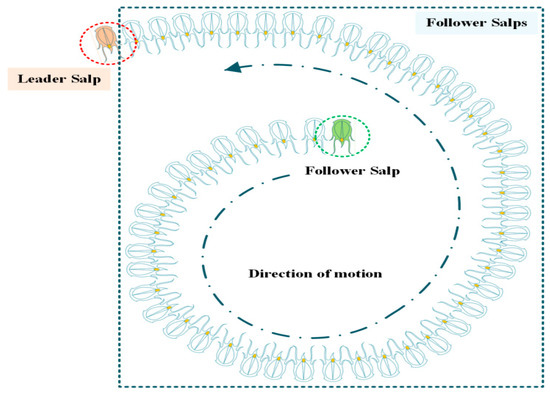
Figure 21. Salp chain (or a swarm of salps).

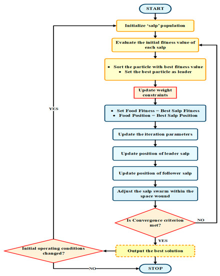
Figure 22. Flowchart of the SSA MPPT strategy.

Initially, update the candidate solutions for the leader and then update the followers̛ candidate solutions by making use of the solutions obtained for leaders. In L_m,t consider m = 1, 2, …, M and t = 1, 2, …, N, which signifies initial candidate solutions for the whole chain. Here, M and N symbolize the size of the salp chain and the number of decision variables, respectively.

Candidate Solution for the leaders:

The candidate solutions for the leaders are updated by employing Equation (38).

$$\left\{\begin{array}{c}{L}_{m,t}{}^{new}=P_t+d_1\left(\left(L_t{}^{+}-L_t{}^{-}\right)d_2+L_t{}^{-}\right)d_3\ge 0.5\\ L_{m,t}{}^{new}=P_t-d_{1 }\left(\left(L_t{}^{+}-L_t{}^{-}\right)d_2+L_t{}^{-}\right)d_3<0.5\end{array}\right.$$

(38)

where L_m,t^new is the updated candidate solution for L_m,t; P_t is the food source position, L_t⁺ and L_t⁻ signify the maximum and minimum values of Decemberision variables, d₁ is adjusted duringiterations, and d₂ and d₃ are random numbers distributed uniformly in the range [0, 1],as per Equation (39)

$$d_1=2e^{-{\left(4\mathrm{i}/I\right)}^2}$$

(39)

where I indicate the maximum count of the iterations, ‘i’ denote the current iteration.

Candidate Solutions for Followers:

The candidate solution of the leaders assists in updating the candidate solutions for the followers. Equation (40) estimates the new candidate solutions for the followers.

$$L_{m,t}{}^{new}=\frac{L_{m,t}+L_{m-1,t}}{2}$$

(40)

where $L_{m,t}{}^{new}$ denotes the updated candidate solution for the follower $L_{m,t}.$ In case candidate solutions of the whole chain violate the minimum and maximum values of decision variables even after modification as suggested in Equations(38) and (40), there is a need to reinitialize the candidate solutions at the respective minimum and maximum values of decision variables [61].

Steps involved in implementing the SSA technique:

• Step_1: Initialize salps’ population L_m,t such that m = 1, 2, …, M, and t = 1, 2, …, N.
• Step_2: Assess thewhole population
• Step_3: Identifythe fittest salp, i.e., P
• Step_4: Modify d₁ using Equation (39)
• Step_5: Update candidate solutions for leaders using (38)
• Step_6: Update candidate solutions for followers using (40)
• Step_7: Modify the candidate solutions breaching the maximum and minimum values of Decemberision variables
• Step 8: Print the corresponding result.

(g) 

  Jaya Algorithm

The Jaya Algorithm (JA) was proposed by R. Venkata Rao in 2015 [62]. The JA strategy is an easy global optimization technique. The JA assists in solving the constrained and unconstrained issues. As there is no learning phase involved in the JA technique, it can implement a parameter-free system, since there is no learning phase involved [63].

The JA helps in solving a specific problem by chasing the best solution while discarding the worst solution. Furthermore, this algorithm requires few constraints like population size, number of design variables, and the total count of generations. The flowchart of JA is demonstrated in Figure 23.

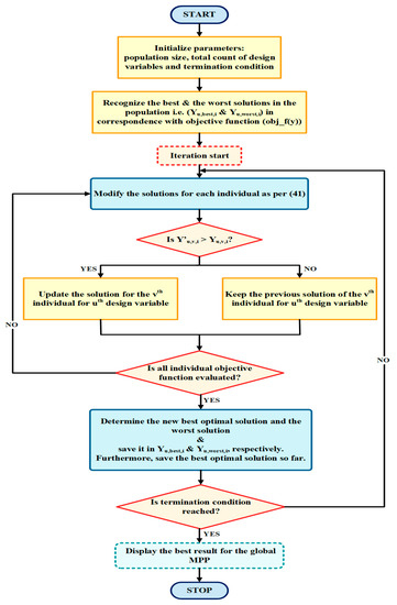
Figure 23. Flowchart of the JA MPPT strategy.

The working rule of the JA strategy involves the following steps:

• Step_1: Initialization of the population size, the total count of designed variables, and the termination condition.
• Step_2: Repeat Step3 to Step5 until the termination condition is fulfilled.
• Step_3: Evaluate the solutions for the objective function.

The prime aim of the optimization problem is to minimize or maximize the objective function (here obj_f(y)). At the ith iteration, N indicates the total count of candidate solution (i.e., u = 1, 2, 3, …, N) and M represents the total count of design variables (i.e., v = 1, 2, 3, …, M). Moreover, for the ith iteration count, obj_f(y)_best and obj_f(y)_worst indicate the best and worst solutions among the individuals. Let $Y_{u,best,i}$ and $Y_{u,worst,i}$ stand for the best and worst solutions for the uth design variable at the ith iteration, respectively. The random numbers $r_{1,v,i}$ and $r_{1,v,i}$ lie in the range [0, 1]. The random numbers aid in the movement of the candidates. These direct candidates toward the best solution and away from the worst solution by utilizing $r_{1,v,i}\left(Y_{u,best,i}-\left|Y_{u,v,i}\right|\right)$ and $(-r_{2,v,i}\left(Y_{u,wost,i}-\left|Y_{u,v,i}\right|\right))$, respectively.

• Step_4: Compute the modified solution utilizing Equation (41).

$${Y^{\prime }}_{u,v,i}=Y_{u,v,i}+r_{1, v, i}\left(Y_{u, best, i}-\left|Y_{u,v,i}\right|\right)-r_{2, v, i}\left(Y_{u, wost, i}-\left|Y_{u,v,i}\right|\right)$$

(41)

• Step_5: Update the previous solution, if Y′_u,v,i > Y′_u,v,i. Otherwise, the previous solution is retained.
• Step_6: Display the final best solution.

The Jaya algorithm is better than conventional techniques regarding efficiency and tracking time parameters during the PSC conditions.

Table 2. The latest research work in the domain of swarm intelligence MPPT techniques.

Authors, Year	Strategies Involved	Control Parameter	DC-DC Converter	Controller Implementation	Findings/Remarks
L. Zaghba, et al. [64], 2021	PSO + FLC MPPT algorithm	Fuzzy gain	Boost converter	MATLAB/Simulink	In the PSO-Fuzzy method, the PSO strategy finds the gain of the controllers. The suggested hybrid algorithm operates at the high tracking speed and shows low oscillation at GMPP compared to classical methods.
Z. E. Hariz, et al. [65], 2021	PSO + GA + P&O MPPT method	PID regulatory parameters	Buck-Boost converter	MATLAB/Simulink	In the hybrid strategy considering the merits of P&O, PSO, and the GA methods, PSO is applied to generate the first population of the GA to decrease the GA technique search space. GA method selects the parameters of the PID regulators to optimize the PPV. The proposed hybrid strategy offers fewer ripples, stabilization, and undershoot time in contrast to the PSO and GA techniques during rapidly changing atmospheric conditions.
G. Krishnan, et al. [66], 2020	Modified ACO MPPT technique	Du variation	Boost converter	MATLAB/Simulink	In the initial few tracking stages, the population size of the ants is kept constant to promote the effective food searching process. Hence, it prevents the possibility of trapping in the local minima. Locations far from the immediate optimal solution (i.e., inefficient) are removed in the following search process. Such a reduction process reduces the computational time. The enhanced scheme provides a low tracking time and small power ripples.
K. Rajalashmi, et al. [67], 2018	Ant colony optimization based on new pheromone update (ACO NPU)	Du	Buck-Boost converter	MATLAB/Simulink	ACO NPU strategy refreshes the pheromone in the midst of the search process, advancing the ants to move towards the GMPP. The proposed algorithm employs a sporadic dispersal look for search progression. Improved accuracy and tracking speed are the advancements shown by the proposed method compared to the traditional ACO.
C. González-Castaño, et al. [68], 2021	Novel ABC MPPT strategy	Du	Boost converter	Digital signal controller (DSC): TI 28069M and high-speed simulator: PLECS RT Box	The proposed novel method requires merely 10% data of the PV module for the training stage. Digital implementation of the novel ABC strategy is easy. Two nested control loops (current loop as internal and voltage loop as outer) aids in regulating the VPV, minimize the steady-state error under varying temperature and solar insolation conditions.
M. R. Fanani, et al. [69], 2020	ABC MPPT strategy	Du	Zeta converter	PSIM Simulator	Zeta converter employment in the MPPT framework results in high accuracy compared to the no-MPPT and traditional human psychology optimization methods. Reduction in the GMPP tracking time.
F. R. Hasan, et al. [70], 2021	GWO with constant power generation (CPG) MPPT strategy	Power limit	SEPIC converter	PSIM software	GWO MPPT-CPG algorithm prevents the occurrence of overvoltage at the load side during varying irradiance conditions.
J. Jayaudhaya, et al. [57], 2020	Multi-objective GWO method	Du	Boost converter	MATLAB/Simulink	Closed-loop control of the PV battery system by utilizing the GWO algorithm is implemented, which improved the power extraction from the PV array.
M. A. Sameh, et al. [59], 2021	EPO MPPT strategy	Du	Boost converter	MATLAB/Simulink and PI controller	The consequences of the PSCs on the PV system can be minimized by employing optimal primary duty cycle settings. For efficient performance of the system under dynamic PSCs, tuning the gains of the duty cycle, PI controller, and the second-order amplifier (SOA) is necessary. The proposed EPO algorithm works effectively for system parameter optimization. Including energy terms in objective function leads to enhancement in tracking speed in contrast with the function considering only output power terms. Ease of implementation.
M. N. I. Jamaludin, et al. [71], 2021	SSO MPPT algorithm	Du	Buck-Boost converter	MATLAB/Simulink, TMS320F28335 DSP controller, Code Composer Studio (CCS)	The proposed algorithm works efficiently under dynamic irradiance conditions as well as PSC conditions. Merely a few steps are required to follow the GMPP. Additionally, it has a simple structure to deal with dynamic conditions. SSA methods surpass the widespread meta-heuristic strategies in all matters, prominently in terms of accuracy and tracking speed. The consequences of the PSCs on the PV system can be minimized by employing optimal primary duty cycles settings. During various atmospheric conditions, SSO algorithm efficiency exceeds 99%.
A. F. Mirza, et al. [72], 2020	SSO MPPT strategy	Du	Buck-Boost converter	MATLAB/Simulink, Atmel ATMEGA-2560	The suggested SSO algorithm is 20–30% quicker than the standard strategies such as PSO, CS, ABC, etc. Short settling times and fast-tracking speeds enable the proposed scheme to save power in a transient state. It also prevents ripples and over-shoot conditions.
H. Deboucha, et al. [73], 2020	Modified JA MPPT method	Du	Boost converter	dSPACE CP1104-TMS320F240 DSP	The proposed Jaya strategy requires only a single tuning parameter need. Hence, algorithm implementation becomes easy, particularly during PSCs. GMPP detection involves a few iterations only, thus reducing the tracking time. Modified Jaya algorithm eliminates the steady-state oscillations. The highest achievable efficiency of the algorithm is 99%.

Table 2. The latest research work in the domain of swarm intelligence MPPT techniques.

Authors, Year	Strategies Involved	Control Parameter	DC-DC Converter	Controller Implementation	Findings/Remarks
L. Zaghba, et al. [64], 2021	PSO + FLC MPPT algorithm	Fuzzy gain	Boost converter	MATLAB/Simulink	In the PSO-Fuzzy method, the PSO strategy finds the gain of the controllers. The suggested hybrid algorithm operates at the high tracking speed and shows low oscillation at GMPP compared to classical methods.
Z. E. Hariz, et al. [65], 2021	PSO + GA + P&O MPPT method	PID regulatory parameters	Buck-Boost converter	MATLAB/Simulink	In the hybrid strategy considering the merits of P&O, PSO, and the GA methods, PSO is applied to generate the first population of the GA to decrease the GA technique search space. GA method selects the parameters of the PID regulators to optimize the PPV. The proposed hybrid strategy offers fewer ripples, stabilization, and undershoot time in contrast to the PSO and GA techniques during rapidly changing atmospheric conditions.
G. Krishnan, et al. [66], 2020	Modified ACO MPPT technique	Du variation	Boost converter	MATLAB/Simulink	In the initial few tracking stages, the population size of the ants is kept constant to promote the effective food searching process. Hence, it prevents the possibility of trapping in the local minima. Locations far from the immediate optimal solution (i.e., inefficient) are removed in the following search process. Such a reduction process reduces the computational time. The enhanced scheme provides a low tracking time and small power ripples.
K. Rajalashmi, et al. [67], 2018	Ant colony optimization based on new pheromone update (ACO NPU)	Du	Buck-Boost converter	MATLAB/Simulink	ACO NPU strategy refreshes the pheromone in the midst of the search process, advancing the ants to move towards the GMPP. The proposed algorithm employs a sporadic dispersal look for search progression. Improved accuracy and tracking speed are the advancements shown by the proposed method compared to the traditional ACO.
C. González-Castaño, et al. [68], 2021	Novel ABC MPPT strategy	Du	Boost converter	Digital signal controller (DSC): TI 28069M and high-speed simulator: PLECS RT Box	The proposed novel method requires merely 10% data of the PV module for the training stage. Digital implementation of the novel ABC strategy is easy. Two nested control loops (current loop as internal and voltage loop as outer) aids in regulating the VPV, minimize the steady-state error under varying temperature and solar insolation conditions.
M. R. Fanani, et al. [69], 2020	ABC MPPT strategy	Du	Zeta converter	PSIM Simulator	Zeta converter employment in the MPPT framework results in high accuracy compared to the no-MPPT and traditional human psychology optimization methods. Reduction in the GMPP tracking time.
F. R. Hasan, et al. [70], 2021	GWO with constant power generation (CPG) MPPT strategy	Power limit	SEPIC converter	PSIM software	GWO MPPT-CPG algorithm prevents the occurrence of overvoltage at the load side during varying irradiance conditions.
J. Jayaudhaya, et al. [57], 2020	Multi-objective GWO method	Du	Boost converter	MATLAB/Simulink	Closed-loop control of the PV battery system by utilizing the GWO algorithm is implemented, which improved the power extraction from the PV array.
M. A. Sameh, et al. [59], 2021	EPO MPPT strategy	Du	Boost converter	MATLAB/Simulink and PI controller	The consequences of the PSCs on the PV system can be minimized by employing optimal primary duty cycle settings. For efficient performance of the system under dynamic PSCs, tuning the gains of the duty cycle, PI controller, and the second-order amplifier (SOA) is necessary. The proposed EPO algorithm works effectively for system parameter optimization. Including energy terms in objective function leads to enhancement in tracking speed in contrast with the function considering only output power terms. Ease of implementation.
M. N. I. Jamaludin, et al. [71], 2021	SSO MPPT algorithm	Du	Buck-Boost converter	MATLAB/Simulink, TMS320F28335 DSP controller, Code Composer Studio (CCS)	The proposed algorithm works efficiently under dynamic irradiance conditions as well as PSC conditions. Merely a few steps are required to follow the GMPP. Additionally, it has a simple structure to deal with dynamic conditions. SSA methods surpass the widespread meta-heuristic strategies in all matters, prominently in terms of accuracy and tracking speed. The consequences of the PSCs on the PV system can be minimized by employing optimal primary duty cycles settings. During various atmospheric conditions, SSO algorithm efficiency exceeds 99%.
A. F. Mirza, et al. [72], 2020	SSO MPPT strategy	Du	Buck-Boost converter	MATLAB/Simulink, Atmel ATMEGA-2560	The suggested SSO algorithm is 20–30% quicker than the standard strategies such as PSO, CS, ABC, etc. Short settling times and fast-tracking speeds enable the proposed scheme to save power in a transient state. It also prevents ripples and over-shoot conditions.
H. Deboucha, et al. [73], 2020	Modified JA MPPT method	Du	Boost converter	dSPACE CP1104-TMS320F240 DSP	The proposed Jaya strategy requires only a single tuning parameter need. Hence, algorithm implementation becomes easy, particularly during PSCs. GMPP detection involves a few iterations only, thus reducing the tracking time. Modified Jaya algorithm eliminates the steady-state oscillations. The highest achievable efficiency of the algorithm is 99%.

6.2.2. Bio-Inspired Algorithm

The following sub-section thoroughly discusses the bio-inspired MPPT techniques. Furthermore, the recent research work related to these methods in the MPPT domain is encapsulated in Table 3.

(a) 

Cuckoo Search MPPT Technique

The Cuckoo Search (CS) technique was suggested by Xin-She Yang and Suash Deb in 2009 [74]. The cuckoo species’ parasitic impersonation strategy (brood-parasitism) [75] is the inspiration behind the CS strategy. Brood parasitism is the conduct of a few cuckoo birds like Tapera. Generally, brood parasitism is classified as intra-explicit, synergetic, and nest takeover [76]. Tapera is a wise winged animal that mirrors the host fowls fit. The fiddle and shading tricks are a part of the host fowl strategy, hence prompting next-generation survival. The CS technique is an efficient meta-heuristic tool for optimization purposes. The flowchart of the CS strategy is illustrated in Figure 24.

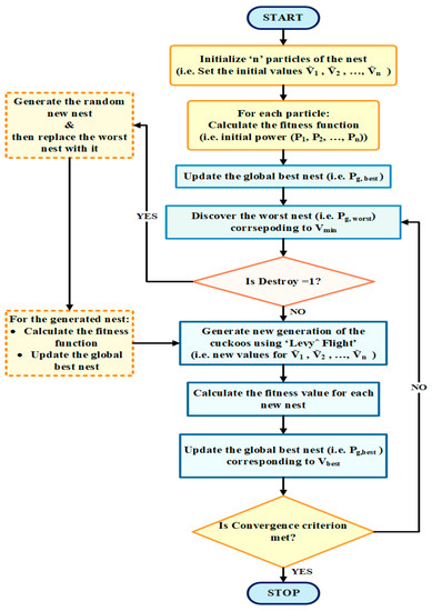
Figure 24. Flowchart of Cuckoo Search technique.

The cuckoo bird comes under the category of parasitic living beings. The cuckoo lays its eggs inside the other flying creatures’ nests as opposed to constructing their nests. Initially, the cuckoo female birds will fly haphazardly to look for the host species’ nest with comparable egg attributes to their own. Afterward, it will pick the best nest with the end goal that their eggs have the most obvious opportunity to bring forth and hence, produce another age of cuckoo. The cuckoo bird will make a few attempts to help the incubating chance by deliberately laying their eggs in a decent position. Sometimes, the cuckoo may throw species eggs from the nest. Host birds could be easily tricked and acknowledge the unfamiliar eggs. By chance, if the host bird finds out about the alien eggs, then the unloading of the eggs outside the nest is sure. In the worst scenario, the host bird may destroy the nest, destroying the alien eggs.

For implementing the CS strategy, the following three idealized standards are utilized.

i.

Each cuckoo bird lays a single egg at a time and puts it in a haphazardly selected host nest;

ii.

The nest withthe best high-quality eggs (i.e., the optimal solutions) will carry forward the next generation of cuckoos;

iii.

The total count of the accessible host nests is fixed in the search space. The likelihood that the host bird will find the foreign egg is denoted by P_f, which lies in the range (0 ≤ P_f ≤ 1).

In the CS strategy implementation, cuckoo birds symbolize the particles relegated to discover the solution. The cuckoo bird’s eggs represent the solution for the present iteration concerning an optimization issue.

The search for the nest is equivalent to the search for food. As Levŷ flight is possibly the most widely recognized model for choosing the walks and directions, it hence later demonstrates certain numerical functions [77]. The Levŷ flight is like a chaotic walk wherein the progression lengths have a probability distribution while steps characterize the progression lengths. The CS algorithm utilizes the power-law to draw the progression length from Levŷ distribution as per the [78].

$$Levŷ\left(\gamma \right) = {Ļ}^{-\gamma }, (1<\gamma <3)$$

(42)

where Ļ denotes the length of the step size, and γ represents the variance, i.e., the power-law index. Hence, Levŷ(γ) function has an infinite variance.

Levŷ flight is characterized by utilizing Equation (43) to generate new solutions (${\tilde{x}}^{i+1}$) for a cuckoo.

$${\tilde{x}}_n^{i+1}=x_n^{~i}+ά ⨶\left( Levŷ\left(\gamma \right)\right)$$

(43)

where n stands for the nth particle, ‘i’ designates the iteration cycle; $(ά$> 0) signifies the step size related to the optimization problem; $⨶$ symbolizes the operator representing the entry-wise multiplication for the multidimensional problem.

For MPPT, the Levŷ flight can be modified as Equation (44) to generate new voltage samples.

$${\mathsf{Ṽ}}_n^{i+1}={\mathsf{Ṽ}}_n^i+\mathsf{ά} ⨶ \left(Levŷ\left(\gamma \right)\right)$$

$${\mathsf{Ṽ}}_n^{i+1}={\mathsf{Ṽ}}_n^i+\mathsf{ά} . \left(Levŷ\left(\gamma \right)\right)$$

$${\mathsf{Ṽ}}_n^{i+1}={\mathsf{Ṽ}}_n^i+K.\left(\frac{a}{{\left|b\right|}^{\frac{1}{\gamma }}}\right).\left({\mathsf{Ṽ}}_{best}-{\mathsf{Ṽ}}_n\right)$$

(44)

where ${\mathsf{Ṽ}}_n^i$ indicates the voltage of the nth particle at the ith iteration; K signifies the coefficient of Levŷ multiplication; and a, b are calculated by the standard distribution curve as depicted in (45).

$$y=N\left(0, {\ddot{\sigma }}_a^2\right); z=N\left(0, {\ddot{\sigma }}_b^2\right)$$

(45)

where

$${\sigma }_a={\left(\frac{\Gamma \left(1+\gamma \right)\times \sin \left(\pi +\gamma /2\right)}{\Gamma \left(\frac{1+\gamma }{2}\right)\times \gamma \times 2^{\frac{\gamma -1}{2}}}\right)}^{\frac{1}{\gamma }}; {\sigma }_b=1$$

(46)

where $\Gamma$ stand for the integral gamma function.

Levŷ flights are conveyed by all the particles in every iteration cycle till they discover the GMPP. If all particles converge to a specific solution, then the tracking process will halt as the best solution is attained.

(b) 

Flying Squirrel Search Optimization Strategy

The flying squirrel search optimization (FSSO) was proposed by Nagendra Singh, Krishna Kumar Gupta, and their colleagues in 2020 [79]. The FSSO strategy impersonates the powerful search strategy of southern flying squirrels. Additionally, the FSSO emulates the squirrels’ way of floating headways in the air exhibited in Figure 25. The probable result vector and the equivalent wellness are alluded to as the stance of a flying squirrel (FS) and are characteristic of food origin, respectively. Based on wellness worth, the stance is grouped into three districts addressing sets of the best solution (BS) (hickory nut tree), close to best solution (CBS) (acorn nut tree), and unplanned solution (US) (ordinary tree).

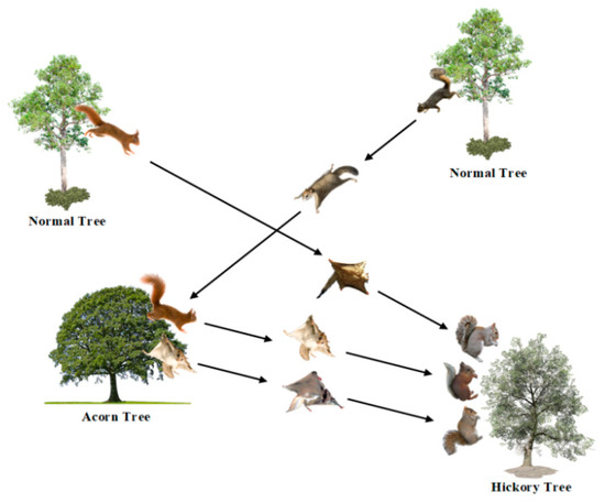
Figure 25. Foraging conduct of flying squirrels.

The FSSO strategy exploits the collaboration feature of the flying squirrels. Moreover, the stances of FSs are updated irrespective of the hunter’s presence. The aforementioned cooperative feature among FSs is the reason for the convergence attribute. This strategy guide by the following steps:

• Step1: CBS moves towards the course chosen by the globally leading solution;
• Step2: Part of USs progress towards the Optimum Solution (OS);
• Step3: The surplus US progresses towards CBS.

The following assumptions are taken into consideration while implementing the FSSO strategy for MPPT:

▪

The aim (food point of supply) resembles the PV power yield (P_PV).

▪

The choice variable, i.e., the stance, is considered a duty ratio (D) of the converter employed in the MPPT technique.

▪

The FSSO strategy is appropriately custom-fitted by wiping out the presence of hunters to lessen the time to reach the GMPP.

The FSSO strategy flowchart is exhibited in Figure 26.

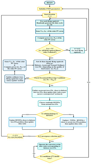
Figure 26. Flowchart of the FSSO MPPT strategy.

The FSSO strategy implementation considers the following step measures:

Starting: At first, the N number of FSs is situated at various positions. These positions in the solution arena are the precise estimations of the converter’s duty ratio per Equation (47).

$$D_i=D_{min}+\frac{\left(i-1\right)\left(D_{max}-D_{min}\right)}{N}; i=1, 2, 3, \dots , N$$

(47)

Here, ‘i’ indicate the iteration count; D_max and D_min depict the maximum and minimum values of the converter’s duty ratio, usually taken as 10% and 90% of allowable duty in the ratio for the boost application. The duty ratio (D_i) can vary in between (0, 0.5).

Wellness Evaluation: In this progression, the converter is progressively working with every duty ratio (i.e., the stance of every FS). For every duty ratio (D), the characteristic of a food source represents the immediate PV power yield P_PV(D) This progression is repeated for all duty cycles, while the goal wellness function (F) for the MPPT is characterized as:

$$F\left(D\right)=max(P_{PV}\left(D\right))$$

(48)

Declaration and Categorization: The duty ratio corresponding to the maximum PV power yield is pronounced as the hickory tree. Acorn trees are viewed as the best stances of the FS. The left-behind FSs reside on the typical trees.

Stance update:The duty cycle update is conveyed in the wake of checking the occasional observing condition. If $(O_C^i-O_{min})$ the duty cycles are refreshed utilizing (i) and (ii). From that point, wellness is assessed.

• Occasional observing conditions: Occasional observing conditions prevent the algorithm from being caught in local maxima. For a solitary dimensional space, the periodic consistent (O_C) and its base worth (O_min) is estimated by:

$$\left\{\begin{array}{c}{O}_C^i = \left|X_{at}^i-X_{ht}\right|\\ O_{\min }=\frac{10e^{-6}}{{365}^{i/(i_m/2.5)}}\end{array}\right.$$

(49)

Here, $X_{at} \mathrm{and} X_{ht}$ address squirrels stance at hickory and acorn trees, individually; ‘i’ symbolizes the current cycle count, and $i_m$ denotes the maximum number of cycles permitted.

The Levy distribution is employed for better hunt arena investigation. Thus, moving the duty ratio of (FSs on ordinary trees) OTFS.

$$X_{ot}^{i+1}=X_{ot}^i+d$$

(50)

Here, $X_{ot}$ address the squirrel stance at ordinary tree and d indicates the step distance, and the utilizing Levy distribution is introduced as:

$$d=\mathsf{Ɛ}\left(\frac{y}{\left|z^{\frac{1}{\gamma }}\right|}\right) \left(X_{ht}-X_{ot}\right)$$

(51)

Here, γ addresses the Levy index, and Ɛ addresses the step coefficient whose values are 1.5 and 1.25, individually. At the same time, y and z are decided from the standard distribution curve, as per Equations (59) and (60).

ii.

Groove contemporized: The hickory tree squirrels abide in their stance. Although, the acorn tree squirrels navigate to approach the hickory tree. However, the erratically chosen squirrel ETFS from ordinary trees navigate toward the hickory tree, while the leftover (NTFS − ETFS) is pushed toward the acorn tree. The comparing duty ratios are refreshed as per the following conditions:

$$D_{at}^{i+1}=D_{at}^i+H_c{h}_d\left(D_{ht}^i-D_{at}^i\right)$$

(52)

$$D_{ot}^{i+1}=D_{ot}^i+H_c{h}_d\left(D_{ht}^i-D_{ot}^i\right)$$

(53)

$$D_{ot}^{i+1}=D_{ot}^i+H_c{h}_d\left(D_{at}^i-D_{ot}^i\right)$$

(54)

Here $H_c \mathrm{and} h_d$ address the hovering constant and hovering distances individually. The estimation of $H_c$ is held to 1.90 after thorough imitations. The hovering distance $h_d$ is estimated as follows:

$$\left\{\begin{array}{c}{h}_d=\frac{z_h}{c_m\tan \propto }\\ \tan \propto =\frac{F_h}{F_r}\end{array}\right.$$

(55)

where $z_h$ signifies the zenith loss after hovering, its value is estimated to be 8 m; $c_m$ stands for the measuring factor whose value is chosen as 18 to keep $h_d$ somewhere in the range of 0.5 and 1.11 to restrict the distress in Equations (52)–(54).Whereas, $F_h\mathrm{and} F_r$ represent the force of the haul and the rise, individually, which are determined as:

$$\left\{\begin{array}{c}{F}_h=\frac{1}{2}{\rho }_a{v}^{2}A{C}_h\\ F_r=\frac{1}{2}{\rho }_a{v}^{2}A{C}_r\end{array}\right.$$

(56)

where ${\rho }_a$ is the air density whose estimation is taken as $1.204 \mathrm{kg}/{\mathrm{m}}^3$; v represents the velocity of a squirrel, whose estimation is taken as $5.25 \mathrm{m}/\mathrm{s}$; furthermore, A is the surface area of the body, which is chosen as $154{ \mathrm{cm}}^2$; $C_h$ is the haul coefficient which is chosen as 0.6, and $C_r$ indicates the rise coefficient whose value is chosen arbitrarily between [0.675, 1.5] [80].

iii.

Convergence Resolution: If the adjustment instance of every FSs evolves into a diminutive ratherthan an edge. Moreover, if the maximum count of iteration has arrived, then in such a case, the improved algorithm is ended and yields the duty cycle at the point at which the converter works while following GMPP.

iv.

Re-Initialization:As the MPPT strategy is the time variation advancement, the frequently changing climate conditions harm the wellness esteem. In the circumstances mentioned above, the FSs stances (i.e., duty ratio) will reinitialize to look for the new GMPP once more. The duty ratio will reinitialize by accompanying the limitation condition as inEquation (57). The reinitialization is in the wake of distinguishing the change in insolation.

$$\frac{P_{PV}^{i+1}-P_{PV}^i}{P_{PV}^{i+1}}\ge ∆P\left(in \%\right)$$

(57)

(c) 

Owl search Algorithm (OSA)

Owls are nocturnal. Irrespective of this, they are skilled predators. They have an auditory system with distinct anatomical features. This feature helps them to hear a sound in one ear before the other. Hence, they can easily detect quarries’ location in the search arena. Furthermore, time and intensity differences in sound wave arrival play a crucial role in estimating their distance to their prey, as illustrated in Figure 27 [81]. The owl search algorithm (OSA) simulates the owl’s hunting method, i.e., relying on the hearing ability in the dark rather than sight to locate the prey. The OSA technique starts with a random arrangement of owls in a search space. This arrangement represents a random set of solutions in a p-dimensional search arena. Here, p indicates the number of variables to be resolved. Matrix (d × p) stores the computed results, as shown in Equation (58).

$$d\times p=\left[\begin{array}{ccc}{W}_{1,1}& \cdots & W_{1,p}\\ ⋮& \ddots & ⋮\\ W_{d,1}& \cdots & W_{d,p}\end{array}\right]$$

(58)

where $W_{n,j}$ signifies the $j_{th}$ initial position (variable) of the $n_{th}$ (the owl), which is determined using a uniform distribution, as given in Equation (59):

$$W_n=W_L+R_P\left(0,1\right)\times \left(W_U-W_L\right)$$

(59)

where $W_U,W_L$ symbolize the upper and lower bounds for the $n_{th}$ owl $(W_n)$, respectively; $R_P\left(0,1\right)$ signifies a random number between [0, 1].

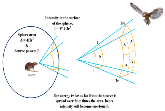
Figure 27. Inverse-square law of sound intensity.

After the application of the random solution, parameter evaluation helps in tracking the optimum solution. Thus, the evaluated parameter aids in enhancing the result in the next cycle. The parameter updates the position of a particular $n_{th}$ owl for a specific fitness function T, as represented in Equation (60).

$$P_n=\raisebox{1ex}{$\left(T_n-f\right)$}\!\left/ \!\raisebox{-1ex}{$\left(k-f\right)$}\right.$$

(60)

Here k, f stand for the maximum and minimum values of the fitness function output saved up to the current iteration. The distance between the current solution and the optimum solution for each owl is computed using Equation (61).

$$C_n=||W_n,M_2||$$

(61)

Here M signifies the best location of the prey (i.e., the optimum solution). Therefore, only the fittest owl can reach it.

Another parameter is calculated by utilizing Equation (62).

$$D_n=\raisebox{1ex}{$\left(I_n\right)$}\!\left/ \!\raisebox{-1ex}{$\left(C_n{}^2\right)$}\right.$$

(62)

Lastly, for the next iteration, the position update of the owls is done by employing Equation (63).

$$\left\{\begin{array}{c}{W}_n{}^{i+1}=W_n{}^i+\mathsf{\mu }\times D_n\left|\beta M-W_n{}^i\right|; p_{oa}<0.5\\ W_n{}^{i+1}=W_n{}^i-\mathsf{\mu }\times D_n\left|\beta M-W_n{}^i\right|; p_{oa}\ge 0.5\end{array}\right.$$

(63)

where $p_{oa}$ stands for the probability of the quarry movement (optimum solution); $\beta$ indicates an arbitrary number uniformly distributed in the range [0, 0.5]; $\mathsf{\mu }$ symbolizes the function constantly decreasing linearly from 1.9 to 0;$p_{oa}$ is set to zero since MPP does not change each cycle (Δn = 0.0001 s). The constants $\beta \mathrm{and} \mathsf{\mu }$ are chosen to be 0.5 and 1.5, respectively [82].

(d) 

  Firefly Algorithm (FFA)

Fireflies are also nocturnal and have a specific light pattern that they use to communicate with each other. Each species has the color of the light they produce. Attraction among the fireflies governs the search pattern of the FFA. The FFA was developed by Xin-She Yang while working in Cambridge in 2008. The attractiveness is equivalent to the brightness. A dim firefly moves toward a brighter firefly. Whereas, if the brightness level of the firefly is the same as that of a particular firefly, it will move randomly [83]. The typical flowchart of the firefly algorithm is demonstrated in Figure 28.

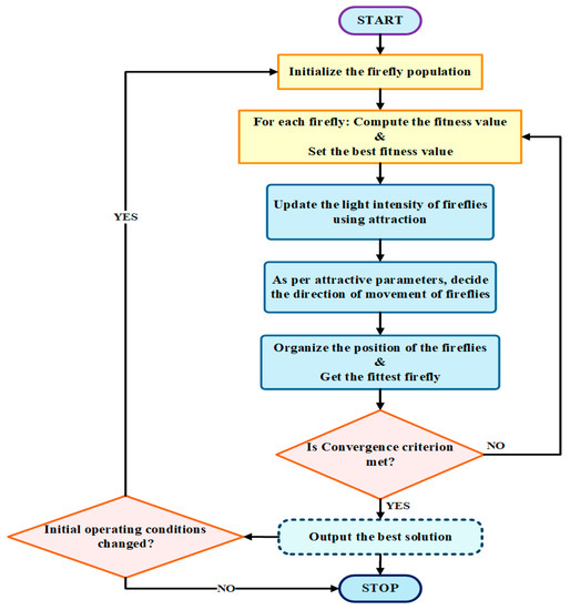
Figure 28. Flowchart of Firefly MPPT strategy.

The FFA strategy has primarily two roles of flickering,

▪

To entice other fireflies.

▪

To lure their prey.

The shine of the fireflies accompanied by the value of the objective function governs the charisma of fireflies. The attraction value of $\mathsf{\mu }$ depends on the estimation of other fireflies. The attraction will differ in accordance with the distance $(d_{ij})$ between the firefly 𝑖 and firefly 𝑗. The attraction of $\mathsf{\mu }$ can be obtained byemploying Equation (64).

$$\mathsf{\mu }={\mathsf{\mu }}_0{e}^{-\beta d^2}$$

(64)

where d indicates the distance between the two fireflies; ${\mathsf{\mu }}_0$ symbolizes the attraction when d = 0 or the initial appeal; β lies in the range [0.1, 10]; the distance between the two fireflies 𝑖 and j at the positions $r_i$ and $r_j$ can be computed by utilizing Equation $\left(65\right).$

$$d_{ij}=\left|r_i-r_j\right|=\sqrt[2]{{{\displaystyle \sum }}_{m=1}^n{(r_{i,m}-r_{j,m})}^2}$$

(65)

where $r_{i,m}$ and $r_{j,m}$ denote m-components in the spatial coordinates of the it^h firefly and the jth firefly; n denotes the dimension number. Since the MPPT problem is a 1-dimensional case, hence d = 1 is utilized. Brighter fireflies entice the dull fireflies, which govern the movement of dull fireflies as per Equation (66).

$$r_i=r_i \mathsf{\mu }(r_i-r_j) + \pounds (rand - \frac{1}{2})$$

(66)

Here £ indicates a random parameter in the range [0, 1]; rand signifies a random disturbance value in between 0 to 1. Generally, large £ leads to the global search, whereas small £ leads to the local search [84].

Table 3. Bio-inspired MPPT algorithms recent research work.

Authors, Year	Strategies Involved	Control Parameter	DC-DC Converter	Controller Implementation	Findings/Remarks
S. Akram, et al. [85], 2021	Direct control CS method	Du	-	MATLAB/Simulink	Direct control CS technique is structured by removing the two PI controllers (i.e., voltage and current controllers) from the traditional CS method. Increment in the accuracy and convergence speed in comparison with the direct control method.
A. Raj, et al. [86], 2021	Improved PSO and CS MPPT algorithms	Du	Boost converter	MATLAB	The combination of a soft computing MPPT control framework with an efficient power converter enhances the performance of the PV systems. In the case of the PSCs, the examined CS MPPT arrangement produces improved results compared to the conventional algorithms.
N. Singh, et al. [79], 2020	FSSO MPPT strategy	Du	Quasi-Z-source Converter	MATLAB/Simulink	Absence of realization of predator leads to faster convergence by the FSSO strategy. In most of cases, the tracking efficiency of the proposed algorithm is highest. The suggested algorithm can be implemented on different infrastructure, and hence it is system independent.
A. F. Farhan, et al. [81], 2019	OSA + P&O MPPT strategy	Du	Boost converter	MATLAB/Simulink	Combining the OSA with P&O enhances the performance of the latter. OSA strategy finds the duty cycle value solutions close to the optimal one, which aids the P&O in following the MPP quickly and steadily without oscillations. Hybrid algorithm implementation cost is equal to the conventional P&O algorithm.
S. N. Altamimi, et al. [87], 2021	OSA + INC MPPT strategy	Du	Boost converter	MATLAB/Simulink	The proposed hybrid scheme improves the convergence speed and tracks the MPP accurately during standard temperature conditions with a slight change in it too. Implementation of the algorithm is easy, and it prevents oscillations at the MPP.
M. Zhang, et al. [88], 2020	FA + vaccine database MPPT strategy	Du	-	MATLAB/Simulink	The modified algorithm eliminates the undesirable individuals from the group and performs the exploration process effectively. Such a modification is possible by modifying the FA strategy iteration term and by adding a database of vaccines with immune replacement progression. The proposed scheme tracking time is less than FA by 2–3 times. An enhanced algorithm tracks the MPP more accurately.
J. Farzaneh, et al. [89], 2020	Modified FA MPPT method	Du	Boost converter	MATLAB/Simulink	Modified FA strategy increases the convergence speed by linearly reducing the algorithm constants per iteration. The average efficiency of the proposed method is greater than 99.98% during the PSC condition.

Table 3. Bio-inspired MPPT algorithms recent research work.

Authors, Year	Strategies Involved	Control Parameter	DC-DC Converter	Controller Implementation	Findings/Remarks
S. Akram, et al. [85], 2021	Direct control CS method	Du	-	MATLAB/Simulink	Direct control CS technique is structured by removing the two PI controllers (i.e., voltage and current controllers) from the traditional CS method. Increment in the accuracy and convergence speed in comparison with the direct control method.
A. Raj, et al. [86], 2021	Improved PSO and CS MPPT algorithms	Du	Boost converter	MATLAB	The combination of a soft computing MPPT control framework with an efficient power converter enhances the performance of the PV systems. In the case of the PSCs, the examined CS MPPT arrangement produces improved results compared to the conventional algorithms.
N. Singh, et al. [79], 2020	FSSO MPPT strategy	Du	Quasi-Z-source Converter	MATLAB/Simulink	Absence of realization of predator leads to faster convergence by the FSSO strategy. In most of cases, the tracking efficiency of the proposed algorithm is highest. The suggested algorithm can be implemented on different infrastructure, and hence it is system independent.
A. F. Farhan, et al. [81], 2019	OSA + P&O MPPT strategy	Du	Boost converter	MATLAB/Simulink	Combining the OSA with P&O enhances the performance of the latter. OSA strategy finds the duty cycle value solutions close to the optimal one, which aids the P&O in following the MPP quickly and steadily without oscillations. Hybrid algorithm implementation cost is equal to the conventional P&O algorithm.
S. N. Altamimi, et al. [87], 2021	OSA + INC MPPT strategy	Du	Boost converter	MATLAB/Simulink	The proposed hybrid scheme improves the convergence speed and tracks the MPP accurately during standard temperature conditions with a slight change in it too. Implementation of the algorithm is easy, and it prevents oscillations at the MPP.
M. Zhang, et al. [88], 2020	FA + vaccine database MPPT strategy	Du	-	MATLAB/Simulink	The modified algorithm eliminates the undesirable individuals from the group and performs the exploration process effectively. Such a modification is possible by modifying the FA strategy iteration term and by adding a database of vaccines with immune replacement progression. The proposed scheme tracking time is less than FA by 2–3 times. An enhanced algorithm tracks the MPP more accurately.
J. Farzaneh, et al. [89], 2020	Modified FA MPPT method	Du	Boost converter	MATLAB/Simulink	Modified FA strategy increases the convergence speed by linearly reducing the algorithm constants per iteration. The average efficiency of the proposed method is greater than 99.98% during the PSC condition.

6.2.3. Artificial Intelligent (AI) Methods

The AI techniques reviewed are grouped as depicted in Figure 29. A comprehensive review of the AI algorithms is addressed in the following sub-sections, while the latest work related to these strategies is sum up in the tabular form in Table 4.

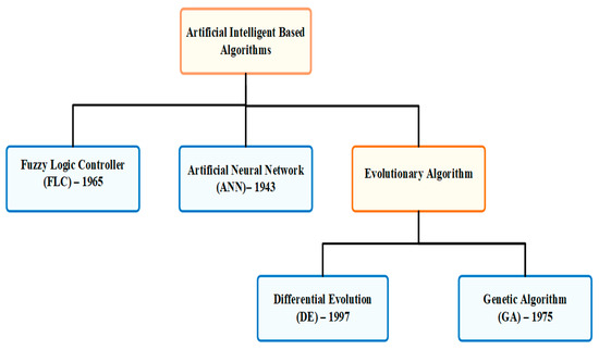
Figure 29. Reviewed AI strategy categorization.

(a) 

Fuzzy Logic Controller Strategy

Fuzzy Logic Controller (FLC) is a control system based on fuzzy logic which converts analog inputs into continuous digital values of0 and 1. For each sample, the FLC strategy analyzes the PV output power. In each case, the change ratio is more than zero. Then the algorithm will adjust the duty cycle of the Pulse Width Modulation (PWM) to increase the voltage. This enhancement in voltage leads to the maximum power ratio outcome to be zero (∆′p/∆′v = 0). Whereas, when the change is less than zero, the algorithm modifies the duty cycle of the PWM to reduce the voltage until the power reaches the pinnacle.

The error and the change in error are the two inputs of the FLC algorithm. The PWM signal controls the boost converter and serves as the output of the strategy. The two input variables: FLC error (E) and error change (∂′E), during times samples (k_i), can be computed using Equations (67) and (68), respectively.

$$E\left(k\right)=\frac{∆\prime {\mathrm{P}}_{\mathrm{pv}}}{∆\prime {\mathrm{V}}_{\mathrm{pv}}}=\frac{\mathrm{Ppv}\left(\mathrm{k}\right)-{\mathrm{P}}_{\mathrm{pv}}\left(\mathrm{k}-1\right)}{{\mathrm{V}}_{\mathrm{pv}}\left(\mathrm{k}\right)-{\mathrm{V}}_{\mathrm{pv}}\left(\mathrm{k}-1\right)}$$

(67)

∂′E(k) = E(k) − E(k − 1)

(68)

Here, P_pv(k) and V_pv(k) symbolize the power and the voltage of the PV panel, respectively.

The FLC strategy consists of three steps: fuzzification, fuzzy rules, and de-fuzzification. In the first step, the input variables transform into linguistic variables by implementing various defined membership functions. In the next step, these variables are manipulated based on the rules “if-then” by applying the desired behavior of the system. Lastly, these variables are renewed to numerical variables. The membership functions are significant in affecting the speed and accuracy of FLC [90].

FLC effectively tracks the maximum power point under different ambient conditions. The FLC strategy shows less oscillation around the MPP. Moreover, its response is faster in comparison with the conventional methods [91]. Furthermore, it has a higher tracking efficiency in contrast to the traditional MPPT methods [92]. The block diagram implementation of the FLC strategy is depicted in Figure 30.

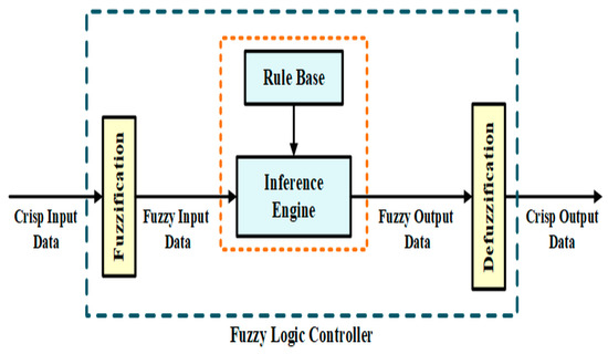
Figure 30. FLC MPPT strategy control block diagram.

• Demerits:

Difficulty in deriving fuzzy rules and this strategy is time-consuming; inability to automatically learn from the environment; complex calculations; undesirable performance under PSC; and fuzzy rules directly affect system performance.

(b) 

 Artificial Neural Network Strategy

The artificial neural network (ANN) is a collection of statistical learning models. The ANN technique emulates the biological neural network for predicting an accurate output per input. Neurons are the basic units of the network which are interlinked. Consequently, neurons process the inflowing data.

A neural network has three layers: input layer, hidden layer, and output layer, as depicted in Figure 31. The total count of neurons in each layer is variable and problem-dependent.

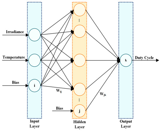
Figure 31. Construction of the ANN.

ANNs are operated as maximum power point tracking systems to foretell the optimum power or voltage produced at a distinct instance. The predicted value acts as a reference that aids in determining the duty cycle. The input variables take into account the PV module parameters and atmospheric parameters. Later, hidden layers in the network process these input variables.

The ANN algorithm provides an enhanced method to diminish the total error (É), as demonstrated in Equation (69).

$$É=\frac{1}{2}\sum {\left({Ŏ}_i-{ť}_i\right)}^i$$

(69)

where I indicates the ith network; $Ŏ$ denotes the actual output; $ť$ symbolizes the estimated outcome.

The breeding algorithm is retrospective in nature and drives a blunder. Later, it feeds back to the output through the input neurons utilizing the centered (covered up) layer neurons. The total number of hidden neurons present is computed by employing Equation (70).

$${Ń}_h=\frac{1}{2}\left({Ń}_I+{Ń}_{°}\right)+\sqrt{{Ń}_t}$$

(70)

where ${Ń}_h$ stands for the count of hidden neurons; ${Ń}_I$ symbolizes the total count of the input neurons injected in the system; ${Ń}_{°}$ denotes the total count of output neurons; ${Ń}_t$ indicates the total count of training samples.

The hardware and simulation setup helps in collecting essential data. Subsequently, the dataset is acquired by inputting solar irradiances, temperatures, PV voltage, or current to the ANN for finding the corresponding P_max or V_max output.

These data are converted to the training data. Later, it passes into the designed ANN to teach it how to perform.

Furthermore, the input data functions transform as the training data for the designed ANN model. The ANN model teaches itself how to perform. After the training part, the test datasets evaluate the performance of the designed ANN, and the errors are fedback to ANN until the weights of all the neurons are adjusted accordingly.

For a particular application, the network needs to be trained by training algorithms. Hence, the system’s overall performance relies on factors like the training process, activation function, and the number of neurons in the hidden layer. Moreover, the quality of the training datasets defines the accuracy of the network.

The feed-forward topology-based ANN consists of three network layers, which is discussed in [93]. As per the simulation results, the ANN-based MPPT algorithm is more accurate than the MPPT algorithm without ANN during solar irradiation and temperature variation. It is proven to have a better response time and less oscillation around MPP [94]. Artificial Neural Network performance improves with an increase in the number of training samples.

However, an accurate, standardized, and proper training set is the main limitation for the ANN to perform optimally without a high training error [95]. ANN requires periodic tuning to cope with the aging and degradation problem of the solar cells [96].

ANN strategy shows a fast response, fast-tracking speed, small steady-state oscillations, and there is even no need to re-program it. However, it requires a massive dataset, which makes its implementation complex and time-consuming.

Evolutionary Computational Strategies

(a) 

Genetic Algorithm

Genetic algorithms (GA) are computational models motivated by evolution.GA comprises chromosomes. These chromosomes encode the possible solution to a problem. Each chromosome carries a distinct set of attributes, i.e., a solution for the application of recombination operators to conserve vital information. GA operates as a function optimizer. To date, GA has been implemented in a broad range of applications. The main reasons for the popularity of GAs in search and optimization problems are their widespread applicability, their global perspective, and their inherent parallelism [91]. GA helps in enhancing the PV voltages and hence generates the maximum power transfer (P_MPP). The simulation result creates an array of data containing voltage (V_pv), power (P_pv), and current (I_PV). In GA, V_pv searches for optimized solutions represented by chromosomes, while Ppv represents the fitness value of a particular chromosome.

The principal concept is to perform genetic alterations (selection, crossover, mutation, and insertion) on a population of individuals. Eventually, an ideal individual is obtained, corresponding to the maximum of the function (i.e., fitness function). The usual flowchart of GA is depicted in Figure 32.

Figure 32. Flowchart of the GA strategy.

The steps of GA strategy execution are as follows:

• Initialization: initially, an arbitrary population with Ń binary individuals is generated with a length Decemberision (bits number Ṡ, exactness). The population consists of a binary matrix (71) in which the count of lines addresses the number of individuals, whereas the column number symbolizes the length of individuals.

  $$\begin{gathered} POP\left(I\right)=\left[\begin{array}{ccc}& \cdots & \\ ⋮& \ddots & ⋮\\ & \cdots & \end{array}\right]\}\begin{array}{l}Ń\\ \mathrm{individuals}\end{array} \\ ⏟ \\ Ṡ\mathrm{bits} \end{gathered}$$

  (71)
  • Assessment:
  • In this appraisal process, the possibility of an individual to be picked is decided by the fitness function $(\widehat{ft) }$ value, so it is a crucial step. In the case of MPPT, the fitness function is the power of the PV module (i.e., P_pv). For each individual, the fitness function is computed, and then its value is utilized to produce a new generation by taking the current value as the parent population as per the fitness function.
  • Genetic Functioning:
  • The operations employed in this step are the foundation of the GA strategy. These do not reject the probability hypotheses, yet they give fascinating tasks; these tasks are:
  • Selection:
    The selection method employed is known as the roulette wheel selection. The probability $({ṕ}_k)$ of the kth individual to be picked is computed by utilizing Equation (72).

    $${ṕ}_k=\frac{\widehat{f{t}_k}}{{{\displaystyle \sum }}_{x=1}^{x=Ń}\widehat{f{t}_x}}$$

    (72)
  • Crossover:
    In this operation, reproduction is performed by crossing the pairs of individuals to produce the novel ones (i.e., children).
  • Mutation:
    In this process, mutation analogous to the biological one is applied. The alteration of one or more genes occurs in a chromosome with the likelihood of change in the random bit from its original form.
  • Insertion:
    It is a replacement process in which the new population is integrated with the previous group of individuals. Later, the individuals withpoor fitness function values are replaced.
  • Program End:
  • Eventually, the algorithm produces a new population consisting of the best individuals. The program will terminate after reaching the desired output as per the system.

GA has relatively small oscillations and rapid convergence speed, and unlike conventional MPPT, GA-based MPPT is capable of searching GMPP instead of being trapped in the local MPP [97,98].

(b) 

Differential Evolution

A Differential Evolution (DE) strategy was suggested by Storn and Price in 1996, specifically for global optimization problems [99]. DE execution is simple as it requires only two parameters, such as a population of particles and a maximum iteration needed to yield the optimal result. Besides, DE has global search space. Therefore, it is employed to follow the GMPP in the case of partial shading conditions. Moreover, the mutation stage in each cycle utilizes distinct attributes of the particles. The flowchart of the DE algorithm is illustrated in Figure 33.

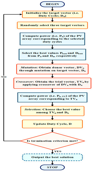
Figure 33. The flowchart of the DE MPPT strategy.

The DC-DC converter’s duty cycle (D) is required to be regulated efficiently to operate the PV system at the GMPP. Hence, the DE strategy utilizes the duty cycle as the target vector, D_n.

At first, a two-dimensional target vector is initialized in DE implementation, with D_n as the populace for each iteration and generation, as shown in Equation (73). After one generation, three particles are selected randomly to decrease the DE strategy execution time.

$${\mathrm{D}}_{\mathrm{g},\mathrm{n}}; \mathrm{n}=1, 2, 3 \dots \mathrm{N}$$

(73)

Subsequently, the chosen duty cycles compute the corresponding power (P_n) of the PV array. Afterwards, the maximum power in the set of 𝑃_n is chosen as 𝑃_best, and the relating 𝐷_n is selected as 𝐷_best. Next, a mutation factor (M) utilizes the weight distinction between the two chosen target vectors. Later, the mutated particle, known as the donor vector (DV_n), is formed by adding the weighted deviation to the third target vector. This interface elucidates the opposition lead between the individuals in life. Hence, the interface promotes local learning from the distinct attributes of one another in the group. Later, this leads to the generation of better individuals to guarantee the advancement of society.

The direction of mutation should guarantee the convergence towards 𝑃_best, which is achieved by employing comparison depicted in Equation (74).

$$D{V}_{g,n}=\left\{\begin{array}{c}{D}_{g,n1}-M\times \left|D_{g,n2}-D_{g,n3}\right|; if D_{g,n1}\ge D_{best}\\ D_{g,n1}+M\times \left|D_{g,n2}-D_{g,n3}\right|; else.\end{array}\right.$$

(74)

where M lies in the range [0, 1].

After mutation, a process known as the crossover is employed to produce the trial vectors (TV_n) by mixing donor vectors and target vectors, as described in Equation (75). In this process, an arbitrary number (i.e., rand), which lies in the scope of [0, 1], contrasts with the hybrid rate HR, which lies in the range [0, 1].

$$T{V}_n=\left\{\begin{array}{c}D{V}_n; if rand\ge HR \\ D_n; else.\end{array}\right.$$

(75)

Later, we estimated the powers of the PV array corresponding to trial vectors; P_n,TV. Notwithstanding, after the crossover process, the value of TV_n may remain the same as D_n and subsequently P_n,TV is likewise equivalent to P_n. Hence, the power P_n,TV corresponding to the duty cycle is different to that of P_n and is estimated again by employing a DC-DC converter. This interaction assists with lessening the search time.

As forthe correlation, the duty cycle directing the optimum power is utilized as the new TV as per Equation (76).

$$D_{n+1}=\left\{\begin{array}{c}{D}_{n,TV}; if{P}_{n,TV}\ge P_n\\ D_n; else.\end{array}\right.$$

(76)

Therefore, the course of action is continued from the mutation production until a convergence condition is fulfilled.

Table 4. Previous research is done in the artificial intelligence MPPT strategies domain.

Authors, Year	Strategies Involved	Control Parameter	DC-DC Converter	Controller Implementation	Findings/Remarks
T. Sutikno, et al. [100], 2021	FLC MPPT strategy + Generalized Bell (GBell) membership function	PWM feed	High gain voltage DC-DC converter	MATLAB/Simulink	In terms of optimization of the converter output, tracking speed, and oscillations, the GBell function surpasses other fuzzy membership functions. The shape of the GBell membership function offers outstanding performance for solar photovoltaic systems.
W. S. E. Abdellatif, et al. [101], 2021	Modified FLC algorithm	Fuzzy rule	Boost Converter	MATLAB/Simulink	The proposed FLC control scheme enhances the working of the MPPT algorithm, specifically for the grid-connected PV frameworks. The modified strategy reduces the steady-state oscillations of the power, voltages, and current, resulting in an improvement in the framework’s efficiency.
M. L. Azad, et al. [102], 2020	Fuzzy based Strategy	Du variation	Boost converter	MATLAB/Simulink	The suggested Fuzzy control technique functions in the stable zone all over the entire span of the PV array. Consequently, it eliminates the fluctuations around the MPP. Despite the intricacies of the proposed Fuzzy strategy, it could be efficiently executed using a microcontroller for converters.
A. Raj, et al. [103], 2021	Feed-forward weight updating + INC method for training	Du	Boost converter	soft-computer MPPT controller	The performance of a PV system can be enhanced by employing a powerful power converter and a soft-computer MPPT controller. The modified strategy depicts a good steady-state response and fewer transients.
A. I. Khan, et al. [104], 2021	Modified ANN algorithm	Du	Boost converter	MATLAB/Simulink	The Levenberg–Marquardt algorithm is employed for training purposes. V and I are taken as input parameters and Du as an output parameter in the proposed algorithm. The modified method precisely follows the MPP and the tracking speed is fast compared to conventional ANN.
M. N. Ali, et al. [105], 2021	ANN + Metaheuristic + Fuzzy-Logic Techniques	Change of Du	Boost converter	MATLAB/Simulink	The Fuzzy logic controller is utilized as an MPPT system optimizer, optimized by PSO and GA solvers. GA strategy is employed as the architecture design of ANN-based MPPT. GA-ANN and GA/PSO-FLC-based MPPT techniques show a noteworthy enhancement in the tracking speed and the output DC power. Although the modified strategies are developed for stand-alone PV systems, it can be used for different applications, such as irrigation purposes and for charging an electric vehicle.
M. Jamaiti [106], 2021	Enhanced GA method	Du	Buck-Boost converter	MATLAB/Simulink	Firstly, the GA method is exploited to track the MPP. Lastly, to determine the optimal angle of PV array as per the sun position in the sky. The PI control loop is eliminated, which is applied to influence the duty cycle. The suggested method outperforms the traditional hill-climbing strategy in respect of all atmospheric conditions concerning the steady-state oscillation and tracking speed.
K. H. Chao, et al. [107], 2021	GA + ACO	Du	Boost converter	MATLAB/Simulink	ACO searches the sub-space to avoid tapping in local maxima. GA is executed to find a feasible solution and prevent rushed convergence. Hybrid GA-ACO convergence time is 50% less than that of the GA and ACO techniques. A cross strategy is stable, accurate, and robust.
R. Alayi, et al. [108], 2021	Improved GA strategy	PV panel spatial angel	-	MATLAB/Simulink	Employing a single-axis tracker enhances the PV panel output power. A PV system with a fixed array after optimizing its azimuth and slope angles result in an increase in annual energy production by 0.17%, whereas a PV framework utilizing a single axis following an array leads to an increment of about 0.92%.
M. S. Ahmad, et al. [109], 2021	PSO + DE	V	-	MATLAB/Simulink	PSO-DE implementation in MPPT problems improved the GMPP of the PV array. Noise is canceled in the characteristic curves. Thus, a smooth curve is obtained in the simulation.
K. G. Babu, et al. [110], 2018	Whale Optimization (WO) + DE MPPT strategies	Du	Boost Converter	MATLAB/Simulink	A WO method depicts the prominent searching ability in a wide search zone, while the DE strategy lessens the meta-heuristic nature and random constant effects, resulting in a high convergence speed. The proposed algorithm has a high tracking speed of about two to five times greater than other recent techniques, such as GWO during PSCs and dynamic conditions. The hybrid method is system-independent, reliable, free from initial condition requirements, and quick in all environmental conditions.
K. S. Tey, et al. [111], 2018	Improved DE MPPT strategy	Target vectors	Single-ended primary-inductance converter (SEPIC)	PSIM Electronic Simulation Software and PIC18F4520 microcontroller.	Direct detection of the ISC is by a basic reading of the IPV through decrement and increment in solar irradiance. During changing atmospheric conditions, the proposed algorithm shows a short following time and an increase in power production.

Table 4. Previous research is done in the artificial intelligence MPPT strategies domain.

Authors, Year	Strategies Involved	Control Parameter	DC-DC Converter	Controller Implementation	Findings/Remarks
T. Sutikno, et al. [100], 2021	FLC MPPT strategy + Generalized Bell (GBell) membership function	PWM feed	High gain voltage DC-DC converter	MATLAB/Simulink	In terms of optimization of the converter output, tracking speed, and oscillations, the GBell function surpasses other fuzzy membership functions. The shape of the GBell membership function offers outstanding performance for solar photovoltaic systems.
W. S. E. Abdellatif, et al. [101], 2021	Modified FLC algorithm	Fuzzy rule	Boost Converter	MATLAB/Simulink	The proposed FLC control scheme enhances the working of the MPPT algorithm, specifically for the grid-connected PV frameworks. The modified strategy reduces the steady-state oscillations of the power, voltages, and current, resulting in an improvement in the framework’s efficiency.
M. L. Azad, et al. [102], 2020	Fuzzy based Strategy	Du variation	Boost converter	MATLAB/Simulink	The suggested Fuzzy control technique functions in the stable zone all over the entire span of the PV array. Consequently, it eliminates the fluctuations around the MPP. Despite the intricacies of the proposed Fuzzy strategy, it could be efficiently executed using a microcontroller for converters.
A. Raj, et al. [103], 2021	Feed-forward weight updating + INC method for training	Du	Boost converter	soft-computer MPPT controller	The performance of a PV system can be enhanced by employing a powerful power converter and a soft-computer MPPT controller. The modified strategy depicts a good steady-state response and fewer transients.
A. I. Khan, et al. [104], 2021	Modified ANN algorithm	Du	Boost converter	MATLAB/Simulink	The Levenberg–Marquardt algorithm is employed for training purposes. V and I are taken as input parameters and Du as an output parameter in the proposed algorithm. The modified method precisely follows the MPP and the tracking speed is fast compared to conventional ANN.
M. N. Ali, et al. [105], 2021	ANN + Metaheuristic + Fuzzy-Logic Techniques	Change of Du	Boost converter	MATLAB/Simulink	The Fuzzy logic controller is utilized as an MPPT system optimizer, optimized by PSO and GA solvers. GA strategy is employed as the architecture design of ANN-based MPPT. GA-ANN and GA/PSO-FLC-based MPPT techniques show a noteworthy enhancement in the tracking speed and the output DC power. Although the modified strategies are developed for stand-alone PV systems, it can be used for different applications, such as irrigation purposes and for charging an electric vehicle.
M. Jamaiti [106], 2021	Enhanced GA method	Du	Buck-Boost converter	MATLAB/Simulink	Firstly, the GA method is exploited to track the MPP. Lastly, to determine the optimal angle of PV array as per the sun position in the sky. The PI control loop is eliminated, which is applied to influence the duty cycle. The suggested method outperforms the traditional hill-climbing strategy in respect of all atmospheric conditions concerning the steady-state oscillation and tracking speed.
K. H. Chao, et al. [107], 2021	GA + ACO	Du	Boost converter	MATLAB/Simulink	ACO searches the sub-space to avoid tapping in local maxima. GA is executed to find a feasible solution and prevent rushed convergence. Hybrid GA-ACO convergence time is 50% less than that of the GA and ACO techniques. A cross strategy is stable, accurate, and robust.
R. Alayi, et al. [108], 2021	Improved GA strategy	PV panel spatial angel	-	MATLAB/Simulink	Employing a single-axis tracker enhances the PV panel output power. A PV system with a fixed array after optimizing its azimuth and slope angles result in an increase in annual energy production by 0.17%, whereas a PV framework utilizing a single axis following an array leads to an increment of about 0.92%.
M. S. Ahmad, et al. [109], 2021	PSO + DE	V	-	MATLAB/Simulink	PSO-DE implementation in MPPT problems improved the GMPP of the PV array. Noise is canceled in the characteristic curves. Thus, a smooth curve is obtained in the simulation.
K. G. Babu, et al. [110], 2018	Whale Optimization (WO) + DE MPPT strategies	Du	Boost Converter	MATLAB/Simulink	A WO method depicts the prominent searching ability in a wide search zone, while the DE strategy lessens the meta-heuristic nature and random constant effects, resulting in a high convergence speed. The proposed algorithm has a high tracking speed of about two to five times greater than other recent techniques, such as GWO during PSCs and dynamic conditions. The hybrid method is system-independent, reliable, free from initial condition requirements, and quick in all environmental conditions.
K. S. Tey, et al. [111], 2018	Improved DE MPPT strategy	Target vectors	Single-ended primary-inductance converter (SEPIC)	PSIM Electronic Simulation Software and PIC18F4520 microcontroller.	Direct detection of the ISC is by a basic reading of the IPV through decrement and increment in solar irradiance. During changing atmospheric conditions, the proposed algorithm shows a short following time and an increase in power production.

7. Comparison and Analysis

During the uniform irradiance condition, conventional MPPT techniques (i.e., P&O, INC, FOCV, FSCC, etc.) show an efficiency of 99%. However, the traditional strategy competence deceases under the PSC circumstances because of the multiple peaks in the P–V curve. Hence, conventional tracking strategies got stuck at the local maxima. Therefore, to overcome this problem, advanced techniques have been employed such as the meta-heuristic approaches, hybrids, etc. The fundamental principle of the advanced strategies is to yield the maximum power irrespective of the change in irradiation. In this review article, a comparison between the conventional, meta-heuristic, and artificial intelligence algorithms has been made. The comparison of algorithms acknowledges different parameters, such as strategy complexity, convergence speed, tacking accuracy, PV array dependency, etc. The pros and cons, applications, and commercial products of the MPPT techniques are illustrated in Table 5. The comparison of some well-known MPPT strategies based on various factors is depicted in Table 6.

Table 5. Comparison of different MPPT techniques based on: Pros, Cons, Applications, and Commercial Products.

Classification	MPPT Techniques	Advantages	Disadvantages	Applications	Commercial Products
Conventional	Perturb and observe (P&O)	Straight-forward design; ease in execution; and work for both grid-connected and stand-alone systems	Less efficient; oscillates around MPP during steady-state	Stand-alone	Genasun GV Boost charge controller with MPPT
	Incremental conductance (INC)	Good performance during fast-changing weather circumstances; and good noise rejection	Implementation is complex; needs a high computational capacity	Stand-alone	-
	Fractional open-circuit voltage (FOCV)	Simplicity; utilizes only one feedback loop	Power loss due to interrupted system operation when the entire control range is scanned	Stand-alone	-
	Fractional short-circuit current (FSCC)	One feedback loop is employed; and easy computation	Less efficient; short-circuit current proportionality factor varies with the PV module parameters	Stand-alone	-
Metaheuristic	Particle swarm optimization (PSO)	Fast computational capability; MPP location for any sort of P–V curve regardless of the environmental conditions can be easily located; good dynamic response; and reliable	Slow tracking speed; and initial parameters need to be selected carefully	Grid-connected	Morningstar-Trackstar MPPT charge controller, Solar Electric Supply (USA)
	Ant colony optimization (ACO)	Convergence independent of initial conditions, and convergence rate is fast	Difficult Implementation	Grid-connected	Morningstar SS-MPPT-15L SunSaver 15 Amp MPPT Solar Charge Controller.
	Artificial bee colony (ABC)	Independent of the initial condition; Fewer control constraints; and a high tracking speed	Complex Implementation	Grid-connected	Morningstar SG-4 SunGuard 4.5 Amp PWM Charge Controller 12 V.
	Cuckoo search (CS)	High efficiency and fewer tuning parameters	Unspecified parameters	Grid-connected	-
	Grey wolf optimization (GWO)	Highly efficient, transient oscillation elimination, and fast	Initialization is complex; more unknown constraints	Grid-connected	-
	Flying squirrel search algorithm (FSSA)	Faster convergence, Highly efficient, system-independent	When climatic conditions change; re-initialization is needed to search for the new GMPP	Grid-connected	-
	Emperor penguin optimization (EPO)	It can be employed to optimize the parameters of other algorithms.	Initialization dependent	Grid-connected	-
	Salp swarm algorithm (SSA)	Highly efficient; fast; highly accurate	Computational burden	Grid-connected	-
	Jaya Algorithm (JA)	Free from strategyspecific parameters; single learning phase; few control parameters	Random numbers could lead to negative solutions	Grid-connected	-
	Owl search algorithm (OSA)	Simple computation; can be used to optimize other method parameters	Initialization dependent	Grid-connected	-
	Firefly algorithm (FFA)	Easy computational steps; can be implemented using low-cost microcontrollers	The position of each firefly varies in a stepwise manner	Grid-connected	-
Artificial Intelligence	Fuzzy logic control (FLC)	A precise mathematical model is not required, good for time-varying, non-linear systems, and systems lacking proper models	Hardware implementation cost is high	Grid-connected	Morning star-Trackstar MPPT charge controller, Solar Electric Supply, USA
	Artificial neural network (ANN)	Good dynamic performance, fast; tracking accuracy is good; no need to be re-programmed	Small steady-state oscillation; require other algorithms for neural training; periodic tuning required	Grid-connected	Morning star-Trackstar MPPT charge controller, Solar Electric Supply, USA
	Genetic algorithm (GA)	It can be utilized for optimizing parameters of other algorithms such asFLC	Hardware required for its implementation is costly	Grid-connected	-
	Differential evolution (DE)	Convergence independent of initial conditions; and fast convergence	Optimal solution not guaranteed	Grid-connected	-

Table 6. Comparison of MPPT Techniques.

Algorithm Category	MPPT Algorithm	Complexity of Algorithm	Cost of Implementation	Tracking Speed	Tracking Accuracy	Analog/Digital	Sensed Parameters	Steady-State Oscillation	PV Array Dependency
Conventional	P&O	S	AFF	Slow	L	A/D	V, I	La	N
	INC	M	EX	Moderate	M	D	V, I	M	N
	FOCV	S	INEX	Fast	L	A/D	V	La	Y
	FSCC	M	INEX	Fast	L	A/D	I	M	Y
Meta-heuristic	PSO	M	AFF	Moderate	M	A/D	V, I	Var.	N
	ACO	S	INEX	Fast	M	D	V, I	̴ Z	N
	ABC	M-C	EX	Fast	M	D	V, I	̴ Z	N
	CS	S-M	EX	V. Fast	H	D	V, I	̴ Z	N
	GWO	S	AFF	Moderate	H	D	V, I	̴ Z	N
	FSSO	M	EX	Fast	H	D	V, I	̴ Z	N
	EPO	C	INEX	Fast	H	-	Du, T	-	N
	SSA	S	AFF	V. Fast	H	D	V, I	̴ Z	N
	JA	S	INEX	V. Fast	H	D	V	̴ Z	N
	OSA	S	INEX	Fast	H	-	-	̴ Z	N
	FFA	S	AFF	Moderate	H	D	V, I	̴ Z	N
Artificial Intelligence	FLC	C	AFF	Fast	V. H	D	Var.	̴ Z	Y
	ANN	M-C	EX	Moderate	V. H	D	Var.	̴ Z	Y
	GA	C	EX	Moderate	M-H	D	Var.	̴ Z	N
	DE	M	AFF	Moderate	M-H	D	V, I	̴ Z	N

Note: S—Small, M—Medium, C—Complex, AFF—Affordable, EX—Expensive, INEX—Inexpensive, V.—Very, L—Low, H—High, A—Analog, D—Digital, V—Voltage, I—Current, Du—Duty Cycle, T—Temperature, Var.—Varies, La—Large, ̴ Z—Almost Zero, N—No, and Y—Yes

The parameters considered for evaluation are as follows:

i.

Algorithm Complexity

MPPT technique efficiency relies immensely upon its implementation complexity. It decides the accuracy of the computations carried out by the strategy to follow the MPPT. Consequently, the algorithms consisting of simple calculations, such as FSCC, FOCV, etc., have good competence under uniform irradiation conditions, and their execution rate is fast. However, advanced techniques, such as meta-heuristic and artificial intelligence, have complex algorithm designs.

ii.

Implementation

While designing the PV framework, choosing the MPPT technique was a crucial decision. This decision also takes into account the ease in execution of algorithms. Nonetheless, it profoundly depends on the user’s interest and his knowledge of MPPT handling since some may like to manage analog circuits while others may be more skillful in handling computerized systems. Moreover, the MPPT algorithm implementation relies on the count of sensors utilized, the cost, design complexity, and other equipment necessities. Furthermore, some MPPT algorithms require a particular topology for their implementation. Hence, the user should be familiar with the various implementation topologies of the algorithms.

iii.

Cost

The necessity of sensors is more pronounced when climatic conditions change suddenly, as the requirement of sensors and hardware increase in such cases. Additionally, some MPPT algorithms require current measurements. Hence, such strategies must invest in the high venture for its hardware execution as current sensors are costly. Furthermore, the expense of MPPT technique implementation relies upon selecting the circuits, as digital courses are expensive compared to analog ones.

iv.

Following and Convergence Speed

Solar irradiance does not remain constant throughout the day as it varies accordingly with the rapid climate changes. Hence, in such a case, partial shading phenomena may be more pronounced. The PSC leads to multiple peaks in the solar P–V characteristics. Because of this, there is a decrease in the tracking speed and convergence speed of the PV framework. The conventional techniques cannot track the true maxima in a single step because these strategies need iterative advances that sense, compute, and perturbed to follow the GMPP. Therefore, traditional algorithms have a slow tracking speed and advanced techniques like PSO, FLC, etc., are much more efficient for PSC cases. Furthermore, it is essential to take the tracking and convergence speeds into account when designing PV systems.

8. Simulation Results

The Cuckoo Search (CS) and Jaya algorithm (JA) are implemented in MATLAB Simulink software version 2021a.Eventually, the output of the system was measured for varying solar irradiance. The characteristics of the PV module employed in the simulation are listed in Table 7.

Table 7. Specification of the PV module.

Parameter	Value
Number of PV module	4
Maximum Power (PMPP)	35.97 W
Cells per module (Ncell)	36
Open circuit voltage (Voc)	21.4 V
Short-circuit current (Isc)	2.3 A
Voltage at MPP (VMPP)	16.5 V
Current at MPP (IMPP)	2.18 A
Temperature coefficient of Voc	−0.76 (%/°C)
Temperature coefficient of Isc	0.7 (%/°C)

The first simulation was performed by taking solar irradiances of the four panels as 1000, 1000, 300, and 300 W/m² at a temperature of 25 °C. The results of the simulation for CS and JA strategies are illustrated in Figure 34 and Figure 35, respectively. The oscillations from the start of the simulation settle down when the optimum power point gets tracked.

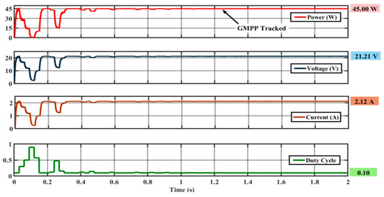
Figure 34. Output power, voltage, and current curve of a PV panel with variations in irradiance as per the first set, and duty cycle curve controlled using CS algorithm.

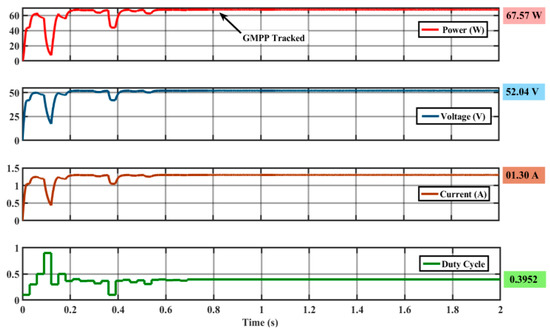
Figure 35. Output power, voltage, and current curve of a PV panel with variation in irradiance as per the first set, and duty cycle curve controlled using the JA algorithm.

The simulation results indicate that JA tracks the maximum power point at 0.7 s, whereas the CS strategy tracks it at 1.2 s. The difference in tracking time signifies that the JA algorithm tracking speed is faster than the CS strategy. Furthermore, the JA strategy tracked down the global optimum power point as 67.57 W. However, the CS technique tracked the MPP as 45 W, which indicates that it is stuck in the local optimum power point. Thus, the JA strategy is more accurate than the CS technique.

For the second simulation, insolation levels of 1000, 800, 600, 400 and 300 W/m² were adjusted to the PV panels. Each panel was set to a temperature of 25 °C. The curve for the variation of the power, voltage, current, and duty cycle with respect to time for the CS algorithm is depicted in Figure 36. The graph for the power indicates that the maximum power tracked was 30.36 W, which is less than the one followed in the first case at 1.2 s. Moreover, the time taken to locate the MPP by the CS strategy is approximately the same in both cases.

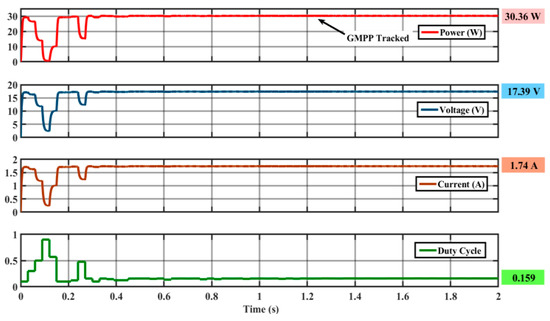
Figure 36. Output power, voltage, and current curve of a PV panel with variation in irradiance as per the second set, and the duty cycle curve was controlled using the CS algorithm.

9. Future Research Work Recommendations

In this article, nineteen cutting-edge MPPT strategies have been reviewed and compared based on different parameters. Moreover, the advantages and disadvantages of each algorithm have been comprehensively discussed, and later, the information was arranged in tabular form. Currently, the PV MPPT algorithm counts exceed more than a hundred, and each year more than five new optimization algorithms are published. Such extensive research works to open the wide area for further reviewing the MPPT algorithms. Hence, this article updates the review articles by analyzing and assessing the well-known methods along with some recent strategies. Additionally, this work presents the latest findings in each algorithm field in the tabulated format.

In the future, the research study can be updated by including:

i.

An analysis of the accuracy of the MPPT techniques during the hot spot process. Since the last Decemberade, the hot spot has emerged as one of the prominent problems affecting the efficiency of the MPPT algorithms.

ii.

For the real-time assessment of the MPPT algorithms, the time period should be about one week/month.

iii.

Moreover, hybrid algorithms can be examined in the future. Asfor now hybrid strategies are ina boom, these methods avoid the disadvantage of two or more algorithms being taken into account. Thus, a combination of different algorithms complements each other.

10. Conclusions

This analysis gives a thorough review of various optimization techniques used in MPPT, which can be classified into three groups: Conventional, Meta-heuristic, and Artificial Intelligence. This article comprises a comprehensive description of operating measures, along with a flowchart depiction of each MPPT strategy. Later, based on the reviewed articles, different MPPT strategies with some more recent ones are assessed while considering the specific factors. The acknowledged factors are algorithm complexity, tracking speed, cost of implementation, sensed parameters, monitoring accuracy, PV array dependency, steady-state oscillation, and analog/digital.

Furthermore, the pros and cons of the MPPT methods are discussed and are later mustered in the tabulated form. Besides, this study suggests that employing MPP controllers is the best way to tackle PSC problems. Hence, this has paved the way for a vast area of research.

The conventional techniques discussed work fine under uniform irradiance conditions and have less algorithm complexity. However, the classical algorithm tracking speeds are slow when compared to the advanced ones. Furthermore, nowadays, intelligent strategies are more pronounced, as these techniques give the best results during PSCs. Furthermore, intelligent algorithms provide ease in data storing and are independent of mathematical computations. On the other hand, meta-heuristic techniques, which are bio-inspired, are compatible with any solar PV system. These strategies require no prior knowledge of the PV panel parameters. To encapsulate, this review article will be a valuable reference for an analyst or a researcher in selecting an MPPT strategy for an explicit purpose.

References

- Husain, M.A.; Tariq, A.; Hameed, S.; Bin Arif, M.S.; Jain, A. Comparative assessment of maximum power point tracking procedures for photovoltaic systems. Green Energy Environ. 2017, 2, 5–17. [Google Scholar] [CrossRef]
- Guangul, F.M.; Chala, G.T. Solar Energy as Renewable Energy Source: SWOT Analysis. In Proceedings of the 4th MEC International Conference on Big Data and Smart City (ICBDSC), Muscat, Oman, 15–16 January 2019. [Google Scholar]
- Selvan, S.; Nair, P.U. A review on Photo Voltaic MPPT algorithms. Int. J. Electr. Comput. Eng. IJECE 2016, 6, 567–582. [Google Scholar]
- Singh, N.; Goswami, A. Study of P-V and I-V Characteristics of Solar Cell in MATLAB/Simulink. Int. J. Pure Appl. Math. 2018, 118, 24. [Google Scholar]
- Xu, L.; Cheng, R.; Yang, J. A New MPPT Technique for Fast and Efficient Tracking under Fast Varying Solar Irradiation and Load Resistance. Int. J. Photoenergy 2020. [Google Scholar] [CrossRef]
- Kchaou, A.; Naamane, A.; Koubaa, Y.; Sird, N.K.M. Review of different MPPT techniques for a photovoltaic generation systems. J. Autom. Syst.Eng. 2017, 11, 195–207. [Google Scholar]
- Mandadapu, U.; Vedanayakam, S.; Thyagarajan, K. Effect of temperature and irradiance on the electrical performance of a pv module. Int. J. Adv. Res. 2017, 5, 2018–2027. [Google Scholar] [CrossRef]
- Apoorva, G.V.S.; Manohar, T.G.; Uma, B.R. Performance Characteristics of solar cells in Space under Shadow Effect. Int. J. Eng. Res. Appl. 2017, 7, 9–15. [Google Scholar]
- Kumar, V.; Kumar, P.; Srinivasa, S.; Puranik, C.R. Study the Effect of Partial Shading in Solar Photovoltaic System. Int. J. Eng. Res. Technol. IJERT 2019, 7, 1–5. [Google Scholar]
- Djalab, A.; Bessous, N.; Rezaoui, M.M.; Merzouk, I. Study of the effects of Partial Shading on PV Array. In Proceedings of the International Conference on Communications and Electrical Engineering (ICCEE), El Oued, Algeria, 17–18 December 2018. [Google Scholar]
- Patel, H.; Gupta, M.; Bohre, A.K. Mathematical Modeling and Performance Analysis of MPPT based Solar PV System. In Proceedings of the International Conference on Electrical Power and Energy Systems (ICEPES), Bhopal, India, 14–16 December 2016. [Google Scholar]
- Nkambule, M.; Hasan, A.; AliJ, A. Proportional study of Perturb & Observe and Fuzzy Logic Control MPPT Algorithm for a PV system under different weather conditions. In Proceedings of the IEEE 10th GCC Conference and Exhibition, Kuwait, Kuwait, 19–23 April 2019. [Google Scholar]
- Nabipour, M.; Razaz, M.; Seifossadat, S.G.H.; Mortazavi, S.S. A new MPPT scheme based on a novel fuzzy approach. Sci. Direct J. Renew. Sustain. Energy Rev. 2017, 74, 1147–1169. [Google Scholar] [CrossRef]
- Azad, M.L.; Sadhu, P.K.; Das, S.; Satpati, B.; Gupta, A.; Arvind, P.; Biswas, R. An Improved Approach to Design A Photovoltaic Panel. Indones. J. Electr. Eng. Comput. Sci. 2017, 5, 515–520. [Google Scholar] [CrossRef][Green Version]
- Femia, N.; Petrone, G.; Spagnuolo, G.; Vitelli, M. Optimization of Perturb and Observe Maximum Power Point Tracking Method. IEEE Trans. Power Electron. 2005, 20, 963–973. [Google Scholar] [CrossRef]
- PSzemes, T.; Melhem, M. Analyzing and modeling PV with ‘P&O’ MPPT Algorithm by MATLAB/SIMULINK. In Proceedings of the IEEE conference on International Symposium on Small-scale Intelligent Manufacturing Systems (SIMS), Gjovik, Norway, 10–12 June 2020. [Google Scholar]
- Abdelsalam, A.K.; Massoud, A.M.; Ahmed, S.; Enjeti, P. High-performance adaptive perturb and observe MPPT technique for photovoltaic- based microgrids. IEEE Trans. Power Electron. 2011, 26, 1010–1021. [Google Scholar] [CrossRef]
- Guiza, D.; Ounnas, D.; Soufi, Y.; Bouden, A.; Maamri, M. Implementation of Modified Perturb and Observe Based MPPT Algorithm for Photovoltaic System. In Proceedings of the 1st International Conference on Sustainable Renewable Energy Systems and Applications (ICSRESA), Tebessa, Algeria, 4–5 December 2019. [Google Scholar]
- Jain, K.; Gupta, P.M.; Bohre, D.A.K. Implementation and Comparative Analysis of P&O and INC MPPT Method for PV System. In Proceedings of the IEEE International Conference on Power Electronics (IICPE), Jaipur, India, 13–15 December 2018. [Google Scholar]
- Azad, M.L.; Sadhu, P.K.; Das, S. Comparative Study Between P&O and Incremental Conduction MPPT Techniques: A Review. In Proceedings of the International Conference on Intelligent Engineering and Management (ICIEM), London, UK, 17–19 June 2020. [Google Scholar] [CrossRef]
- Mustafić, D.; Jokić, D.; Lale, S.; Lubura, S. Implementation of Incremental Conductance MPPT Algorithm in Real Time in Matlab/Simulink Environment with Humusoft MF634 Board. In Proceedings of the 9th Mediterranean Conference on Embedded Computing (MECO), Budva, Montenegro, 8–11 June 2020. [Google Scholar]
- Femia, N.; Petrone, G.; Spagnuolo, G.; Vitelli, M. Power Electronics and Control Techniques for Maximum Energy Harvesting in Photovoltaic Systems; CRC Press: Boca Raton, FL, USA, 2013. [Google Scholar]
- Murtaza, A.F.; Sher, H.A.; Chiaberge, M.; Boero, D.; Giuseppe, M.D.; Addoweesh, K.E. Comparative Analysis of Maximum Power Point Tracking Techniques for PV applications. In Proceedings of the IEEE International Conference on Multi Topic, Lahore, Pakistan, 19–20 December 2013. [Google Scholar]
- Atri, P.K.; Modi, P.S.; Gujar, N.S. Comparison of Different MPPT Control Strategies for Solar Charge Controller. In Proceedings of the International Conference on Power Electronics & IoT Applications in Renewable Energy and its Control (PARC), Mathura, India, 28–29 February 2020. [Google Scholar]
- Baroi, S.; Sarker, P.C.; Baroi, S. An Improved MPPT Technique—Alternative to Fractional Open Circuit Voltage Method. In Proceedings of the International Conference on Electrical & Electronic Engineering (ICEEE), Rajshahi, Bangladesh, 2–29 December 2017. [Google Scholar]
- Nyarko, I.O.; Elgenedy, M.A.; Ahmed, K. Combined Temperature and Irradiation Effects on the Open Circuit Voltage and Short Circuit Current Constants for Enhancing their Related PV-MPPT Algorithms. In Proceedings of the IEEE Conference on Power Electronics and Renewable Energy (CPERE), Eswan, Egypt, 23–25 October 2019. [Google Scholar]
- Danoune, M.B.; Djafour, A.; Gougui, A.; Khelfaoui, N.; Boutelli, H. Study and Performance Analysis of Three Conventional MPPT Algorithms Used in Photovoltaic Applications. In Proceedings of the International Conference on Communications and Electrical Engineering (ICCEE), El Oeud, Algeria, 17–18 December 2018. [Google Scholar]
- Osman, M.H.; Ahmed, M.K.; Refaat, A.; Korovkin, N.V. A Comparative Study of MPPT for PV System Based on Modified Perturbation & Observation Method. In Proceedings of the 2021 IEEE Conference of Russian Young Researchers in Electrical and Electronic Engineering (ElConRus), St. Petersburg/Moscow, Russia, 26–29 January 2021. [Google Scholar] [CrossRef]
- Raiker, G.A.; Loganathan, U.; Reddy, S.B. Current Control of Boost Converter for PV Interface With Momentum-Based Perturb and Observe MPPT. IEEE Trans. Ind. Appl. 2021, 57, 4071–4079. [Google Scholar] [CrossRef]
- Manna, S.; Akella, A.K. Comparative analysis of various P & O MPPT algorithm for PV system under varying radiation condition. In Proceedings of the 2021 1st International Conference on Power Electronics and Energy (ICPEE), Bhubaneswar, India, 2–3 January 2021. [Google Scholar] [CrossRef]
- Sarika, P.E.; Jacob, J.; Mohammed, S.; Paul, S. A Novel Hybrid Maximum Power Point Tracking Technique with Zero Oscillation based on P&O Algorithm. Intern. J. Renew. Energy Res. IJRER 2020, 10, 1962–1973. [Google Scholar]
- Ounnas, D.; Guiza, D.; Soufi, Y.; Maamri, M. Design and Hardware Implementation of Modified Incremental Conductance Algorithm for Photovoltaic System. Adv. Electr. Electron. Eng. 2021, 19, 100–111. [Google Scholar]
- Hebchi, M.; Kouzou, A.; Choucha, A. Improved Incremental conductance algorithm for MPPT in Photovoltaic System. In Proceedings of the 2021 18th International Multi-Conference on Systems, Signals & Devices (SSD), Monastir, Tunisia, 22–25 March 2021. [Google Scholar] [CrossRef]
- Siddique, M.A.B.; Asad, A.; Asif, R.M.; Rehman, A.U.; Sadiq, M.T.; Ullah, I. Implementation of Incremental Conductance MPPT Algorithm with Integral Regulator by Using Boost Converter in Grid-Connected PV Array. IETE J. Res. 2021, 1–14. [Google Scholar] [CrossRef]
- Ali, M.N.; Mahmoud, K.; Lehtonen, M.; Darwish, M.M.F. An Efficient Fuzzy-Logic Based Variable-Step Incremental Conductance MPPT Method for Grid-Connected PV Systems. IEEE Access. 2021, 9, 26420–26430. [Google Scholar] [CrossRef]
- Baimel, D.; Tapuchi, S.; Levron, Y.; Belikov, J. Improved Fractional Open Circuit Voltage MPPT Methods for PV Systems. Electronics 2019, 8, 321. [Google Scholar] [CrossRef]
- Krishnan, M.M.; Bharath, K.R. A Novel Sensorless Hybrid MPPT Method Based on FOCV Measurement and P&O MPPT Technique for Solar PV Applications. In Proceedings of the 2019 International Conference on Advances in Computing and Communication Engineering (ICACCE), Sathyamangalam, India, 4–6 April 2019; pp. 1–5. [Google Scholar] [CrossRef]
- Bharath, K.R.; Suresh, E. Design and Implementation of Improved Fractional Open Circuit Voltage Based Maximum Power Point Tracking Algorithm for Photovoltaic Applications. Intern. J. Renew. Energy Res. IJRER 2017, 7, 1108–1113. [Google Scholar]
- Fapi, C.B.N.; Wira, P.; Kamta, M. Real-Time Experimental Assessment of a New MPPT Algorithm Based on the Direct Detection of the Short-Circuit Current for a PV System. In Proceedings of the 19th International Conference on Renewable Energies and Power Quality (ICREPQ’21), Almeria, Spain, 28–30 July 2021; Volume 19, pp. 598–603. [Google Scholar] [CrossRef]
- Sher, H.; Murtaza, A.F.; Noman, A.; Addoweesh, K.E.; Chiaberge, M. An intelligent control strategy of fractional short circuit current maximum power point tracking technique for photovoltaic applications. J. Renew. Sustain. Energy 2015, 7, 013114. [Google Scholar] [CrossRef]
- Liu, Y.-H.; Huang, S.-C.; Huang, J.-W.; Liang, W.-C. A Particle Swarm Optimization-Based Maximum Power Point Tracking Algorithm for PV Systems Operating Under Partially Shaded Conditions. IEEE Trans. Energy Convers. 2012, 27, 1027–1035. [Google Scholar] [CrossRef]
- Koad, R.B.A.; Zobaa, A.; El-Shahat, A. A Novel MPPT Algorithm Based on Particle Swarm Optimization for Photovoltaic Systems. IEEE Trans. Sustain. Energy 2016, 8, 468–476. [Google Scholar] [CrossRef]
- Shi, Y.; Eberhart, R. A modified particle swarm optimizer. In Proceedings of the IEEE international conference on IEEE world congress on computational intelligence, evolutionary computation proceedings, IEEE, Anchorage, AK, USA, 4–9 May 1998; pp. 69–73. [Google Scholar]
- Xu, L.; Cheng, R.; Xia, Z.; Shen, Z. Improved Particle Swarm Optimization (PSO)-based MPPT Method for PV String under Partially Shading and Uniform Irradiance Condition. In Proceedings of the 2020 Asia Energy and Electrical Engineering Symposium (AEEES), Chengdu, China, 29–31 May 2020. [Google Scholar] [CrossRef]
- Ratnaweera, A.; Halgamuge, S.; Watson, H.C. Self-Organizing Hierarchical Particle Swarm Optimizer With Time-Varying Acceleration Coefficients. IEEE Trans. Evol. Comput. 2004, 8, 240–255. [Google Scholar] [CrossRef]
- Chen, X.; Chai, Y.; Wang, Y. Application of Adaptive Particle Swarm Optimization in Multi-peak MPPT of Photovoltaic Array. In Proceedings of the IEEE 4th Information Technology, Networking, Electronic and Automation Control Conference (ITNEC), Chongqing, China, 12–14 June 2020. [Google Scholar]
- Dorigo, M.; Stützle, T. Ant colony optimization: Overview and recent advances. In Handbook of Metaheuristics; Springer: Boston, MA, USA, 2019; pp. 311–351. [Google Scholar]
- Kumar, P.M.U.; Devi, G.D.; Manogaran, G.; Sundarasekar, R.; Chilamkurti, N.; Varatharajan, R. Ant colony optimization algorithm with internet of vehicles for intelligent traffic control system. Comput. Netw. 2018, 144, 154–162. [Google Scholar] [CrossRef]
- Jiang, L.L.; Maskell, D.L.; Patra, J. A novel ant colony optimization-based maximum power point tracking for photovoltaic systems under partially shaded conditions. Energy Build. 2013, 58, 227–236. [Google Scholar] [CrossRef]
- Phanden, R.K.; Sharma, L.; Chhabra, J.; Demir, H.I. A novel modified ant colony optimization based maximum power point tracking controller for photovoltaic systems. Mater. Today Proc. 2020, 38, 38–93. [Google Scholar] [CrossRef]
- Karaboga, D.; Basturk, B. A powerful and efficient algorithm for numerical function optimization: Artificial bee colony (ABC) algorithm. J. Glob. Optim. 2007, 39, 459–471. [Google Scholar] [CrossRef]
- Benyoucef, S.; Chouder, A.; Kara, K.; Sahed, Q.A.; Silvestre, S. Artificial bee colony based algorithm for maximum power point tracking (MPPT) for PV systems operating under partial shade. Appl. Soft Comput. 2015, 32, 38–48. [Google Scholar] [CrossRef]
- Mohapatra, A.; Nayak, B.; Das, P.; Mohanty, K.B. A review on MPPT techniques of PV system under partial shading condition. Renew. Sustain. Energy Rev. 2017, 80, 854–867. [Google Scholar] [CrossRef]
- Okula, Ş.; Aksub, D.; Orman, Z. Investigation of Artificial Intelligence Based Optimization Algorithms. J. Istanb. Sabahattin Zaim Univ. Nat. Sci. Inst. 2019, 1, 11–16. [Google Scholar]
- Mirjalili, S.; Mirjalili, S.M.; Lewis, A. Grey wolf optimizer. Adv. Eng. Softw. 2018, 69, 46–61. [Google Scholar] [CrossRef]
- Eltamaly, A.M.; Farh, H.M. Dynamic global maximum power point tracking of the PV systems under variant partial shading using hybrid GWO-FLC. Sol. Energy 2018, 177, 306–316. [Google Scholar] [CrossRef]
- Jayaudhayal, J.; Rajasekaran, D.; Sumithra, J.; Vinitha, J.C.; Karkuzhali, S. Closed Loop Control of PV System Using Grey Wolf Optimization Algorithm under Partial Shading Condition. In Proceedings of the International Conference on Recent Developments in Robotics, Embedded and Internet of Things (ICRDREIOT), Tamil Nadu, India, 16–17 October 2020. [Google Scholar] [CrossRef]
- Dhiman, G.; Kumara, V. Emperor penguin optimizer: A bio-inspired algorithm for engineering problems. Knowledge-Based Syst. 2018, 159, 20–50. [Google Scholar] [CrossRef]
- Sameh, M.A.; Marei, M.I.; Badr, M.A.; Attia, M.A. An Optimized PV Control System Based on the Emperor Penguin Optimizer. Energies 2021, 14, 751. [Google Scholar] [CrossRef]
- Faris, H.; Mirjalili, S.; Aljarah, I.; Mafarja, M.; Heidari, A.A. Salp Swarm Algorithm: Theory, Literature Review, and Application in Extreme Learning Machines. Springer Ser. Fluoresc. 2019, 185–199. [Google Scholar] [CrossRef]
- Patnana, N.; Pattnaik, S.; Varshney, T.; Singh, V.P. Self-Learning Salp Swarm Optimization Based PID Design of Doha RO Plant. Algorithms 2020, 13, 287. [Google Scholar] [CrossRef]
- Huang, C.; Zhang, Z.; Wang, L.; Song, Z.; Long, H. A novel global maximum power point tracking method for PV system using Jaya algorithm. In Proceedings of the IEEE Conference on Energy Internet and Energy System Integration, Beijing, China, 26–28 November 2017. [Google Scholar]
- Zitar, R.A.; Al-Betar, M.A.; Awadallah, M.A.; Doush, I.A.; Assaleh, K. An Intensive and Comprehensive Overview of JAYA Algorithm, its Versions and Applications. Springer Arch. Comput. Methods Eng. 2021. [Google Scholar] [CrossRef]
- Zaghba, L.; Khennane, M.; Borni, A.; Fezzani, A. Intelligent PSO-Fuzzy MPPT approach for Stand Alone PV System under Real Outdoor Weather Conditions. Alger. J. Renew. Energy Sustain. Dev. 2021, 3, 1–12. [Google Scholar]
- El Hariz, Z.; Hicham, A.; Mohammed, D. A novel optimiser of MPPT by using PSO-AG and PID controller. Int. J. Ambient. Energy 2021. [Google Scholar] [CrossRef]
- Krishnan, G.; Kinattingal, S.; Simon, S.P.; Srinivasa, P.; Nayak, R. MPPT in PV systems using ant colony optimization with dwindling population. IET Renew. Power Gener. 2020, 14, 1105–1112. [Google Scholar] [CrossRef]
- Rajalashmi, C.K.; Monisha, C. Maximum Power Point Tracking Using Ant Colony Optimization for Photovoltaic System Under Partially Shaded Conditions. Int. J. Eng. Adv. Technol. IJEAT 2018, 8, 82–87. [Google Scholar]
- Gonzalez-Castano, C.; Restrepo, C.; Kouro, S.; Rodriguez, J. MPPT Algorithm Based on Artificial Bee Colony for PV System. IEEE Access 2021, 9, 43121–43133. [Google Scholar] [CrossRef]
- Fanani, M.R.; Sudiharto, I.; Ferdiansyah, I. Implementation of Maximum Power Point Tracking on PV System using Artificial Bee Colony Algorithm. In Proceedings of the 2020 3rd International Seminar on Research of Information Technology and Intelligent Systems (ISRITI), Yogyakarta, Indonesia, 10 December 2020; pp. 117–122. [Google Scholar] [CrossRef]
- Hasan, F.R.; Prasetyono, E.; Sunarno, E. A Modified Maximum Power Point Tracking Algorithm Using Grey Wolf Optimization for Constant Power Generation of Photovoltaic System. In Proceedings of the 2021 International Conference on Artificial Intelligence and Mechatronics Systems (AIMS), Bandung, Indonesia, 28–30 April 2021; pp. 1–6. [Google Scholar] [CrossRef]
- Jamaludin, M.N.I. An Effective Salp Swarm Based MPPT for Photovoltaic Systems Under Dynamic and Partial Shading Conditions. IEEE Access 2021, 9, 34570–34589. [Google Scholar] [CrossRef]
- Mirza, A.F.; Mansoor, M.; Ling, Q.; Yin, B.; Javed, M.Y. A Salp-Swarm Optimization based MPPT technique for harvesting maximum energy from PV systems under partial shading conditions. Energy Convers. Manag. 2020, 209, 112625. [Google Scholar] [CrossRef]
- Deboucha, H.; Mekhilef, S.; Belaid, S.; Guichi, A. Modified deterministic Jaya (DM-Jaya)-based MPPT algorithm under partially shaded conditions for PV system. IET Power Electron. 2020, 13, 4625–4632. [Google Scholar] [CrossRef]
- Yang, X.; Deb, S. Cuckoo Search via Lévy flights. In Proceedings of the World Congress Nature Biol. Inspired Comput. (NaBIC), Coimbatore, India, 9–11 December2009; pp. 210–214. [Google Scholar]
- Anand, R.; Swaroop, D.; Kumar, B. Global Maximum Power Point Tracking for PV Array under Partial Shading using Cuckoo Search. In Proceedings of the IEEE 9th Power India International Conference (PIICON), Sonepat, India, 28 February–1 March 2020. [Google Scholar]
- Shlesinger, M.F. Search Research. J. Nat. 2006, 443, 281–282. [Google Scholar] [CrossRef]
- Mosaad, M.I.; Raouf, M.O.A.; Al-Ahmar, M.A.; Banakher, F.A. Maximum Power Point Tracking of PV system Based Cuckoo Search Algorithm; review and comparison. Energy Procedia 2018, 162, 117–126. [Google Scholar] [CrossRef]
- Ahmed, N.A.; Rahman, S.A.; Alajmi, B.N. Optimal controller tuning for P&O maximum power point tracking of PV systems using genetic and cuckoo search algorithms. Int. Trans. Electr. Energy Syst. 2020. [Google Scholar] [CrossRef]
- Singh, N.; Gupta, K.K.; Jain, S.K.; Dewangan, N.K.; Bhatnagar, P. A Flying Squirrel Search Optimization for MPPT Under Partial Shaded Photovoltaic System. IEEE J. Emerg. Sel. Top. Power Electron. 2020, 9, 4963–4978. [Google Scholar] [CrossRef]
- Jain, M.; Singh, V.; Rani, A. A novel nature-inspired algorithm for optimization: Squirrel search algorithm. Swarm Evol. Comput. 2019, 44, 148–175. [Google Scholar] [CrossRef]
- Farhan, A.F.; Feilat, E.A.; Al-Salaymeh, A.S. Maximum Power Point Tracking Technique Using Combined Perturb & Observe and Owl Search Algorithms. In Proceedings of the International Conference on Electrical and Computing Technologies and Applications (ICECTA), Ras Al Khaimah, United Arab Emirates, 19–21 November 2019. [Google Scholar]
- Jain, M.; Maurya, S.; Rani, A.; Singh, V. Owl search algorithm: A novel nature-inspired heuristic paradigm for global optimization. J. Intell. Fuzzy Syst. 2018, 34, 1573–1582. [Google Scholar] [CrossRef]
- Palupi, L.N.; Winarno, T.; Pracoyo, A.; Ardhenta, L. Adaptive voltage control for MPPT-firefly algorithm output in PV system. IOP Conf. Series: Mater. Sci. Eng. 2020, 732, 012048. [Google Scholar] [CrossRef]
- Nguyen, T.T.; Quynh, N.V.; Van Dai, L. Improved Firefly Algorithm: A Novel Method for Optimal Operation of Thermal Generating Units. Complexity 2018, 2018, 1–23. [Google Scholar] [CrossRef]
- Akram, S.; Khalil, L.; Bhatti, M.L.; Aftab, T.; Siddique, R.; Riaz, M. Maximum Power Point Tracking using Direct Control with Cuckoo Search for Photovoltaic Module under Partial Shading Condition. Pak. J. Eng. Technol. 2021, 4, 28–31. [Google Scholar] [CrossRef]
- Raj, A.; Gupta, M. Numerical Simulation and Comparative Assessment of Improved Cuckoo Search and PSO based MPPT System for Solar Photovoltaic System Under Partial Shading Condition. Turk. J. Comput. Math. Educ. 2021, 12, 3842–3855. [Google Scholar]
- Altamimi, S.N.; Feilat, E.A.; al Nadi, D.A. Maximum Power Point Tracking Technique Using Combined Incremental Conductance and Owl Search Algorithm. In Proceedings of the 2021 12th International Renewable Engineering Conference (IREC), Amman, Jordan, 14–15 April 2021; pp. 1–6. [Google Scholar] [CrossRef]
- Zhang, M.; Chen, Z.; Wei, L. An Immune Firefly Algorithm for Tracking the Maximum Power Point of PV Array under Partial Shading Conditions. Energies 2019, 12, 3083. [Google Scholar] [CrossRef]
- Farzaneh, J.; Keypour, R.; Khanesar, M.A. A New Maximum Power Point Tracking Based on Modified Firefly Algorithm for PV System Under Partial Shading Conditions. Technol. Econ. Smart Grids Sustain. Energy 2018, 3, 9. [Google Scholar] [CrossRef]
- Al-Majidi, S.D.; Abbod, M.F.; Al-Raweshidy, H.S. A novel maximum power point tracking technique based on fuzzy logic for photovoltaic systems. Int. J. Hydrogen Energy 2018, 43, 14158–14171. [Google Scholar] [CrossRef]
- Issaadi, W.; Mazouzi, M.; Issaadi, S. Command of a Photovoltaic System by Artificial Intelligence, Comparative Studies with Conventional Controls: Results, Improvements, and Perspectives. In Proceedings of the 8th Proceedings of International Conference on Modelling, Identification and Control (ICMIC), Algiers, Algeria, 15–17 November 2017; pp. 583–591. [Google Scholar]
- Mehra, S.; Sharma, R. Performance Analysis of Artificial Intelligence Based MPPT Techniques for a Solar System under Changing Environmental Conditions. In Proceedings of the International Conference on Advances in Electronics, Electrical, and Computational Intelligence (ICAEECA), Allahabad, India, 31 May–1 June 2019. [Google Scholar] [CrossRef]
- Roy, R.B.; Cros, J.; Nandi, A.; Ahmed, T. Maximum Power Tracking by Neural Network. In Proceedings of the 8th International Conference on Reliability, Infocom Technologies and Optimization (Trends and Future Directions) (ICRITO), Noida, India, 4–5 June 2020. [Google Scholar]
- Algarín, C.R.; Hernández, D.S.; Leal, D.R. A Low-Cost Maximum Power Point Tracking System Based on Neural Network Inverse Model Controller. Electronics 2018, 7, 4. [Google Scholar] [CrossRef]
- Al-Majidi, S.D.; Abbod, M.F.; Al-Raweshidy, H.S. Design of an intelligent MPPT based on ANN using a real photovoltaic system data. In Proceedings of the 54th International Universities Power Engineering Conference (UPEC), Bucharest, Romania, 3–6 September 2019; pp. 1–6. [Google Scholar]
- Revathy, S.R.; Kirubakaran, V. A critical review of artificial neural networks based maximum power point tracking techniques. J. Crit.Rev. 2020, 7, 2394–5125. [Google Scholar]
- Mirza, A.F.; Mansoor, M.; Ling, Q.; Khan, M.I.; Aldossary, O.M. Advanced Variable Step Size Incremental Conductance MPPT for a Standalone PV System Utilizing a GA-Tuned PID Controller. Energies 2020, 13, 4153. [Google Scholar] [CrossRef]
- Megantoro, P.; Nugroho, Y.D.; Anggara, F.; Pakha, A.; Pramudita, B.A. The Implementation of Genetic Algorithm to MPPT Technique in a DC/DC Buck Converter under Partial Shading Condition. In Proceedings of the 3rd International Conference on Information Technology, Information Systems and Electrical Engineering (ICITISEE), Yogyakarta, Indonesia, 13–14 November 2018. [Google Scholar]
- Storn, R.; Price, K. Minimizing the real functions of the ICEC’96 contest by differential evolution. In Proceedings of the IEEE International Conference on Evolutionary Computation (ICEC’96), Nagoya, Japan, 20–22 May 1996; pp. 842–844. [Google Scholar]
- Sutikno, T.; Subrata, A.C.; Elkhateb, A. Evaluation of Fuzzy Membership Function Effects for Maximum Power Point Tracking Technique of Photovoltaic System. IEEE Access 2021, 9, 109157–109165. [Google Scholar] [CrossRef]
- Abdellatif, W.S.E.; Mohamed, M.S.; Barakat, S.; Brisha, A. A Fuzzy Logic Controller Based MPPT Technique for Photovoltaic Generation System. Intern. J. Electr. Eng. Inform. 2021, 13. [Google Scholar] [CrossRef]
- Azad, M.L.; Das, S.; Sadhu, P.K.; Arvind, P. High-Performance Algorithms to Ascertain The Power Generation In A Photovoltaic System Using Fuzzy Logic Controller. In Proceedings of the 2020 International Conference on Intelligent Engineering and Management (ICIEM), London, UK, 17–19 June 2020; pp. 425–430. [Google Scholar] [CrossRef]
- Raj, A.; Gupta, M. Numerical Simulation and Performance Assessment of ANN-INC Improved Maximum Power Point Tracking System for Solar Photovoltaic System Under Changing Irradiation Operation. Ann. RSCB 2021, 25, 790–797. [Google Scholar]
- Khan, A.I.; Khan, R.A.; Farooqui, S.A.; Sarfraz, M. Artificial Neural Network-Based Maximum Power Point Tracking Method with the Improved Effectiveness of Standalone Photovoltaic System. In AI and Machine Learning Paradigms for Health Monitoring System: Intelligent Data Analytics; Malik, H., Fatema, N.A.J., Eds.; Springer: Singapore, 2021; Volume 86, pp. 459–470. [Google Scholar]
- Ali, M.N.; Mahmoud, K.; Lehtonen, M.; Darwish, M.M.F. Promising MPPT Methods Combining Metaheuristic, Fuzzy-Logic and ANN Techniques for Grid-Connected Photovoltaic. Sensors 2021, 21, 1244. [Google Scholar] [CrossRef]
- Jamaiti, M. Modeling of Maximum Solar Power Tracking by Genetic Algorithm Method. Iran. J. Energy Environ. IJEE 2021, 12, 118–124. [Google Scholar]
- Chao, K.-H.; Rizal, M. A Hybrid MPPT Controller Based on the Genetic Algorithm and Ant Colony Optimization for Photovoltaic Systems under Partially Shaded Conditions. Energies 2021, 14, 2902. [Google Scholar] [CrossRef]
- Alayi, R.; Harasii, H.; Pourderogar, H. Modeling and optimization of photovoltaic cells with GA algorithm. J. Robot Control. JRC 2020, 2, 35–41. [Google Scholar] [CrossRef]
- Ahmad, M.S.; Ahmad, A. Hybrid PSO-DE Technique to Optimize Energy Resource for PV System. Int. J. Electr. Eng. Technol. IJEET 2021, 12, 128–139. [Google Scholar]
- Babu, K.G.; Kishori, K.R. MPPT design using grey wolf optimization differential evolution (GWODE) technique for partially shaded PV system. Int. J. Emerg. Technol. Innov. Res. 2018, 5, 203–218. [Google Scholar]
- Tey, K.S.; Mekhilef, S.; Seyedmahmoudian, M.; Horan, B.; Oo, A.M.T.; Stojcevski, A. Improved Differential Evolution-Based MPPT Algorithm Using SEPIC for PV Systems Under Partial Shading Conditions and Load Variation. IEEE Trans. Ind. Inform. 2018, 14, 4322–4333. [Google Scholar] [CrossRef]
Publisher’s Note: MDPI stays neutral with regard to jurisdictional claims in published maps and institutional affiliations. |
© 2021 by the authors. Licensee MDPI, Basel, Switzerland. This article is an open access article distributed under the terms and conditions of the Creative Commons Attribution (CC BY) license (https://creativecommons.org/licenses/by/4.0/).