Analyze the FMCW Waveform Skin Return of Moving Objects in the Presence of Stationary Hidden Objects Using Numerical Models

Abstract

In this paper, a high-performance antenna array system model is presented to analyze moving-object-skin-returns and track them in the presence of stationary objects using frequency modulated continuous wave (FMCW). The main features of the paper are bonding the aspects of antenna array and electromagnetic (EM) wave multi-skin-return modeling and simulation (M&S) with the aspects of algorithm and measurement/tracking system architecture. The M&S aspect models both phase and amplitude of the signal waveform from a transmitter to the signal processing in a receiver. In the algorithm aspect, a novel scheme for FMCW signal processing is introduced by combining time- and frequency-domain methods, including a vector moving target indication filter and a vector direct current canceller in time-domain, and a constant false alarm rate detector and a mono-pulse digital beamforming angle tracker in frequency-domain. In addition, unlike previous designs of using M × N fast Fourier transform (FFT) for an M × N array, only four FFTs are used, which tremendously save time and space in hardware. With the presented model, the detection of the moving-target-skin-return in stationary objects under a noisy environment is feasible. Therefore, to track long range and high-speed objects, the proposed technique is promising. Using a scenario having (1) a target with 17 dBm² radar cross section (RCS) at about 40 km range with 5.936 Mach speed and 11.6 dB post processing signal to noise ratio, and (2) a strong stationary clutter with 37 dBm² RCS located at the proximity of the target, it demonstrates that the root-mean-square errors of range, angle, and Doppler measurements are about 26 m, 0.68 degree, and 1100 Hz, respectively.

1. Introduction

Detecting and tracking moving targets’ locations, Doppler frequencies, and velocities based on the target-skin-return is the main function of modern electromagnetic (EM) based tracking and measurement systems, e.g., radars [1]. Successful EM propagation and antenna array modeling for this detection and tracking process in software is important for the designing of such systems for radar electronic warfare studies. In this paper, we present the use of numerical models for analyzing the EM skin return of moving targets in the presence of stationary clutters and receiver noise with Simulink software. The main models include the “point-reflector” target simulation model, the simplified radio frequency (RF) frontend, and the digital beamforming (DBF) receiver. The “point-reflector” target simulation model simulates a target at certain three-dimensional (3D) coordinates using a radar cross section (RCS) number, the 3D coordinates, arbitrary 3D velocities, and arbitrary 3D accelerations as inputs to this model. The simplified RF frontend models transmit-to-receive (TX-to-RX) coupling (or leakage) and the additive white Gaussian noise (AWGN). The features of the paper are to tie the aspects of antenna array and EM wave multi-skin-returns (target and clutter) modeling and simulation (M&S) with the aspects of algorithm and system architecture. It applies the DBF antenna array theory and 3-domain (time-, frequency-, and Doppler-domain) based signal processing theory to the system under design. The numerical models presented in this paper are highly modular. The DBF receiver model is highly parallel by pipeline processing. All the models can be implemented in real time on digital hardware like field programmable gate array (FPGA) and application-specific integrated circuit (ASIC) for real time applications. In the introduction, we first review the recent frequency modulated continuous wave (FMCW) waveform related literature. Then we will address the main contributions of the paper from the modeling and simulation (M&S) aspects, and the FMCW radar algorithm and architecture aspects.

Triangular FMCW waveform [2] is used in this paper as the signal to interrogate moving targets. FMCW waveform has high signal processing gain, due to the continuous transmission and the Fast Fourier Transform (FFT). Two different radio frequency (RF) architectures are available for FMCW systems, as discussed in [3]. The first architecture (p. 9 of [3]) generates a chirp signal in the digital domain for the transmitter and does de-chirping in the digital domain of the receiver. This architecture mixes the received RF waveform with the stable local oscillator signal (the frequency agile part), then mixes the output signal with the coherent oscillator signal (the fixed frequency part), and after that feeds the signal to analog to digital converters (ADCs) [4], then finally, de-chirps the signal in the digital domain. The FMCW algorithm in this paper is based on this architecture. The second architecture (p. 12 of [3]) is to mix the received RF waveform with the transmitted RF waveform, before ADC. This method does de-chirping operation in the RF analog domain. This is a popular architecture used in the automotive industry [5,6,7,8,9,10,11,12,13,14,15] and the harbor surveillance application [16]. In particular, the three-dimensional FFT algorithm per fast time, antenna, and slow time, is very popular for the automotive application in order to estimate the range, angle, and Doppler [11].

From the M&S aspect, typical EM echo measurement system models only present the amplitude level details of the EM wave propagation and radar processing. It uses the radar range equation to calculate the receiver signal to noise ratio, and outputs the detection probability and false alarm probability as system outputs [17]. It also relies on many assumptions made on the radar receiver processing and has very little flexibility. The other approach is to model the complex in-phase and quadrature (I/Q) signals in the radar processing chain. However, simulating the continuous electromagnetic (EM) wave scattering/reflection return (also called skin return) from the targets over the air and across the complex antenna system is often very challenging. Instead of simulating the EM wave interaction with the target using a time domain approach or a frequency domain approach [18,19,20], we use the RCS-based method based on three assumptions. The first assumption assumes that the distance between the rigid body target and the radar is much larger than target size. The second assumption is that the target is at the far field region of the EM wave propagation. The last assumption is that the maximum difference of the distances between any points of the target to the radar is less than half of the product of the receiver sampling time resolution and the speed of light. With these assumptions, we can closely model the target as a moving “point” with 3D coordinates and certain 3D complex valued RCS patterns as a function of the angles in the spherical coordinates. A point target, which represents the “mass center” in the RCS measurement sense (not the physical mass centroid), moves based on its 3D velocity vector and its 3D acceleration vector, and rotates in pitch, roll, and yaw axes [21].

If the radar waveform is band-limited, we can accurately recover the waveform after an arbitrary propagation time using an ideal delay filter based on an adequate number of the non-delayed digital samples [22]. When a target is moving continuously, the coefficients of this ideal delay filter must be changed based on the changes of the EM wave round-trip propagation time. We can describe this continuous target movement using a time varying delay filter and a number of digital samples of the non-delayed waveform. This approach was first introduced in [23].

From the algorithm and architecture aspects, the main novelty of this paper is to use a hybrid time-domain and frequency-domain signal processing architecture, which combines a time domain vector moving target indication (MTI) filter [24,25], a time domain vector direct current (DC) canceller, a frequency domain constant false alarm rate (CFAR) detector [26] and a frequency domain mono-pulse angle tracker [27,28]. The advantages of this new hybrid architecture become obvious when the number of receive antennas is big and the FFT size is large, as in that case the implementation using per-antenna FFT [11] can be dauntingly complex. In our design, we only use four FFTs per target tracker for a 4 × 4 element antenna array. Additionally, each target tracker can be time-multiplexed if properly configured by different targets. The implementation complexity of our approach has been much reduced.

The proposed architecture is a complete tracking and measurement system receiver design with DBF. The input to the system is the initial range, the initial angles in the spherical coordinate system, and the initial Doppler value of the moving target. Then the system does automatic tracking of the angles and calculation of the range and the Doppler. The tracking mechanism uses closed loop mono-pulse tracking, and is different from the open loop tracking while scan (TWS) mechanism [1,29,30]. The MTI filter is a vector extension of the scalar MTI design used for the FMCW radar in [24]. The CFAR detector is similar to the one used in [26]. The mono-pulse tracking follows the previous work in [28]. Compared with our prior work [23], we use the triangular FMCW waveform instead of the sawtooth FMCW waveform, and use vector MTI filter for the clutter cancellation, and the CFAR detector for the target detection. We also present a range extrapolation scheme to extrapolate the range estimate based on the last known range and Doppler values when the target is at the “blind speed” of the vector MTI filter. Additionally, compared with [23], the DC canceller is placed before the beamforming operation to completely cancel the DC and avoid the spectrum sidelobes of the DC caused by the varying beamforming coefficients in time. The proposed architecture can be applied to different radar waveforms, e.g., radar pulses, and even in the joint radar and communications scenario [31], with small modifications.

This paper is organized as follows. In Section 2, we describe the method of simulating the FMCW waveform and the skin-return of a moving target. In Section 3, we introduce the triangular FMCW waveform and describe some basic processing ideas. In Section 4, we present the tracking and measurement system receiver architecture and give details about each receiver block. In Section 5, simulation results about three simulation scenarios are presented. Section 6 gives a brief discussion about the results. Lastly, we draw some conclusions in Section 7.

2. Method of Simulating the FMCW WAVEFORM and the Skin Return of a Moving Target

2.1. The FMCW Tracking and Measurement System Overview

The high level FMCW based tracking and measurement system block diagram is given in Figure 1. A transmitting (TX) antenna beam is formed to illuminate the targets. A receiving (RX) antenna array consisting of $M$ × $N$ antenna elements is used to receive the target skin return signals. A target in the TX antenna beam is considered as a point reflecting source and is modeled by a constant radar cross section (RCS) (σ) in this study. The radar is bi-static. The gains of the TX and RX antennas in the direction of the target are $G_{tR}$ and $G_{rR}$, respectively. The distance between the reference centers of the TX and RX antennas is denoted by $d_{TR}$. The RX antenna is located at the origin of the 3D coordinate system. There exists a power leakage path from the TX antenna to the RX antenna. We assume that the distance between the target and the RX antenna reference center is much bigger than $d_{TR}$.

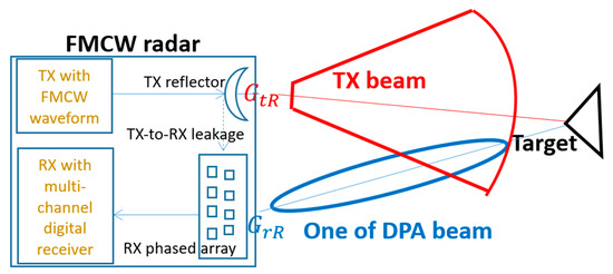
Figure 1. High level frequency modulated continuous wave (FMCW) based tracking and measurement system block diagram. DPA stands for digital phased array.

The radar equation used to model the power-level propagation effect is the bi-static propagation equation. This was used to model the radar received power, as a function of the distance between the radar and its target. The equation is

$$P_r=P_t+G_{tR}+G_{rR}+\sigma +10·{\mathit{log}}_{10}\left(\frac{{\lambda }^2}{{\left(4\pi \right)}^3{R}_{tx}^2{R}_{rx}^2}\right)-L$$

(1)

where $P_r$ is the received signal power in $\mathrm{dBm}$, $P_t$ is the transmitted signal power in $\mathrm{dBm}$, $G_{tR}$ is the transmit antenna gain of the radar in $\mathrm{dBi}$, $G_{rR}$ is the receive antenna gain of the radar in $\mathrm{dBi}$, $\sigma$ is in ${\mathrm{dBm}}^2$, $\lambda$ is the wavelength of the carrier frequency, $R_{tx}$ is the distance between the radar transmitter and the target in meters, $R_{rx}$ is the distance between the radar receiver and the target in meters, and $L$ is the loss in $\mathrm{dB}$. Note that, since targets move, all the parameters in Equation (1) can change with time.

It is also assumed that the RF propagation channel between the TX antenna and each receiving antenna element in the phased array has all-pass characteristics with additive white Gaussian noise (AWGN). This assumption implies that we can simply model the RF path with unit gain, zero delay from the phase reference point of TX antenna to the phase reference center of the RX phased array, and also, the receiving phased array is calibrated to remove all the differences of extra delay, gain, and phase of the RF paths among $M\times N$ receiving channels.

To design and verify the system in computer simulations, we need to model and simulate continuous target movement effects. This is done by using variable delay filters operated on the transmitted waveform, based on the observations from Equation (3). Because of the band-limited property of the transmitted waveform, we only need to delay the in-band signal by a variable delay corresponding to each sample based on the 3D relationship between TX/RX antenna phase centers and the target location, which changes with time.

2.2. RX Coordinate System

The coordinate system in the M&S of the FMCW tracking and measurement system is presented in Figure 2. The panel of the RX phased array is in the XZ-plane, and its phase reference center is at the origin of the Cartesian coordinate. A target is located at $\left(\varphi ,\theta ,R_{rx}\right)$, which is also known as azimuth-angle (Az) (in degrees), elevation-angle (El) (in degrees), and range ($R_{rx}$) (in meters). Since the target moves, the $\left(\varphi ,\theta ,R_{rx}\right)$ values change continuously with time.

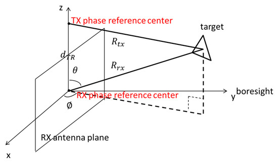
Figure 2. RX (receiving) phased array panel and the target ($R_{rx}$ and $R_{tx}$ are much bigger than $d_{TR}$ in the real system).

2.3. Received Signal Model

The observable range for radar measurement at time $t$ is defined as the average of $R_{tx}\left(t^{\prime }\right)$ and $R_{rx}\left(t^{\prime }\right)$, i.e., $R\left(t\right)=\frac{R_{tx}\left(t^{\prime }\right)+R_{rx}\left(t^{\prime }\right)}{2}$ and $t=t^{\prime }+\frac{R_{rx}\left(t^{\prime }\right)}{c}$, where $t^{\prime }$ is the instance of EM wave that hits the target after the wave leaves the TX phase-center, and $\frac{R_{rx}\left(t^{\prime }\right)}{c}$ is the time interval that is needed when the target echo signal travels backs to the RX phase-center. Where, $c$ is the free space speed of light. Note that, here we assume that the phase-centers of the TX and RX antennas are not collocated. After the two-way propagation, the target echo signal $r\left(t\right)$ is intercepted by the elements in the RX phased array. At the $\left(m,i\right)$^th element, the received analog signal in the complex format can be expressed as

$$r_{mi}\left(t\right)=g_{mi}^c·e^{2\pi j\left(f_c\left(t-\frac{2R\left(t\right)}{c}\right)\right)}·x\left(t-\frac{2R\left(t\right)}{c}\right)$$

(2)

where $g_{mi}^c$ is the complex gain coefficient of the $\left(m,i\right)$^th element, and $x\left(t\right)$ is the transmitted waveform. The received signal is then directly down-converted by the RF front-end, and digitized by ADC at the sampling rate of $f_S$. The sampled signal is

$$r_{mi}\left(k{T}_s\right)=g_{mi}^c·e^{2\pi j\left(-\frac{2f_{c}R\left(k{T}_s\right)}{c}\right)}·x\left(k{T}_S-\frac{2R\left(k{T}_s\right)}{c}\right)$$

(3)

where $k$ is the $k^{th}$ time sample step, $T_S=1/f_S$. The complex gain coefficient can be detailed as

$$g_{mi}^c=\sigma ·g^{air}·b_{mi}^c·h_{rf}^c.$$

(4)

where $\sigma$ is the target RCS, $g^{air}$ is the propagation loss defined by the radar equation in Equation (1), $h_{rf}^c$ is the RX RF channel gain, and the beamforming coefficient $b_{mi}^c$ is in Equation (13), which defines the required phase from the $\left(m,i\right)$^th element in the array in order to form the antenna beam in $\left(\varphi ,\theta \right)$ or $\left[a\left(0\right),a\left(1\right)\right]$ $=[\cos \left(\varphi \right)\sin \left(\theta \right), \cos \left(\theta \right)]$ direction, as described in Equation (12). We have assumed that oversampling is done at the ADC. At the receiver, the ADC I/Q samples are down-sampled by a factor of $K$ to the baseband sampling frequency $f_B$, where $K=\frac{f_S}{f_B}$.

2.4. Waveform Interpolation

As shown Equation (3), the round-trip time delay $\frac{2R\left(k{T}_s\right)}{T_{S}c}$ consists of two parts, i.e., an integer delay part $round\left(\frac{2R\left(k{T}_s\right)}{T_{S}c}\right) \mathrm{that} \mathrm{is} \mathrm{in} \mathrm{certain} \mathrm{number} \mathrm{of} T_s,$ and a fractional delay part ${\tau }_f$ within $\left[-0.5,0.5\right]$ of $T_s$, where

$${\tau }_f=\frac{2R\left(k{T}_s\right)}{T_{S}c}-round\left(\frac{2R\left(k{T}_s\right)}{T_{S}c}\right)$$

(5)

A filter with the approximated all pass characteristics in the passband of $\left[-\frac{1}{2K},\frac{1}{2K}\right]$ means that the filter has unit gain and linear phase slope within $\left[-\pi ,\pi \right]$ in its passband. Using the filter in the oversampling domain, we can do interpolation to obtain the required signal phase that relates to the time delay of ${\tau }_f$. This technique is called Lagrange interpolation filter, which can be expressed as

$$h\left(k^{\prime }\right)={\displaystyle \prod }_{l=0,l\ne k^{\prime }}^P\frac{D-l}{k^{\prime }-l}$$

(6)

where $D={\tau }_f+\mathrm{floor}\left(\frac{P}{2}\right), k^{\prime }$ is the $k^{\prime }$th tap of the Lagrange filter, and P is the order of the Lagrange filter. For example, when $K=2$, the interpolation filter for a fractional delay of $0.25$ has a gain and phase response as shown in Figure 3.

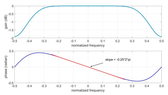
Figure 3. Gain and phase response of a Lagrange filter of order 8 and uniform in-band group delay = 0.25.

Before applying the reflection/scattering gain to the skin return, let us illustrate the post Lagrange interpolation waveform amplitude and phase vs. the fractional delay numbers due to the target movement in Figure 4 and Figure 5. We compare these plots with the post nearest sample interpolation waveform amplitude and phase vs. the fractional delay numbers in Figure 6 and Figure 7. The amplitude and phase in Figure 4 and Figure 5 are computed from the complex differential waveform $r_{diff}\left(k{T}_S\right)$ based on the following equation:

$$r_{diff}\left(k{T}_S\right)=x{\left(k{T}_S-\frac{2R\left(k{T}_s\right)}{c}\right)}^{*}x\left(\left(k-1\right)T_S-\frac{2R\left(\left(k-1\right)T_S\right)}{c}\right)$$

(7)

where ${(·)}^{*}$ stands for conjugate operation. The complex differential waveform $r_{diff}\left(k{T}_S\right)$ represents the phase and amplitude changes of $x\left(k{T}_S-\frac{2R\left(k{T}_s\right)}{c}\right)$ over one $T_S$ duration. Using $r_{diff}\left(k{T}_S\right),$ we can more clearly observe the continuity of the signal $x\left(k{T}_S-\frac{2R\left(k{T}_s\right)}{c}\right)$ in amplitude and phase. If Lagrange interpolation is used, we reconstruct $x\left(k{T}_S-\frac{2R\left(k{T}_S\right)}{c}\right)$ using the Lagrange filtered $x\left(k{T}_S\right)$. If the nearest sample interpolation is used, we approximate $x\left(k{T}_S-\frac{2R\left(k{T}_S\right)}{c}\right)$ by $x\left(\left(k - round\left(\frac{2R\left(k{T}_S\right)}{T_{S}c}\right)\right)T_S\right)$. Clearly, the Lagrange interpolation functions well, with no discontinuity in phase and amplitude after interpolation. The nearest sample interpolation shows an occasional phase discontinuity at $1332.5 T_S$ delay time. Note that the phase discontinuity implies that the simulation with the nearest sample interpolation is inaccurate at the phase jump instance.

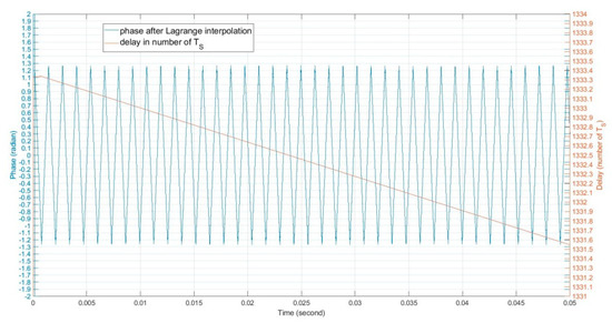
Figure 4. The post Lagrange interpolation waveform phase vs. the fractional delay numbers. No phase jump observed in this figure.

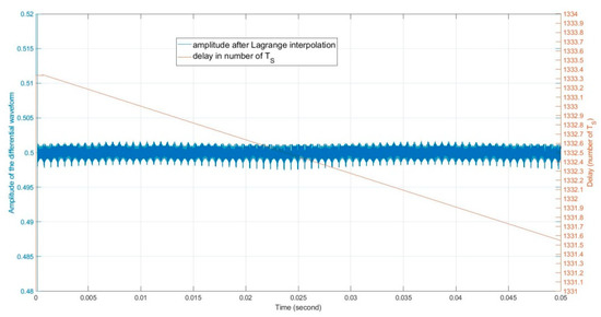
Figure 5. The post Lagrange interpolation waveform amplitude vs. the fractional delay numbers.

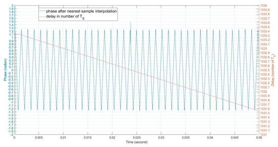
Figure 6. The post nearest sample interpolation waveform phase vs. the fractional delay numbers. A phase discontinuity/jump happens when the delay number is 1332. $5 T_S$ within 0.05 s of simulation time. The phase jump happens when the delay number is $\left(n_{delay}+0.5\right)T_S$, where $n_{delay}$ is an integer.

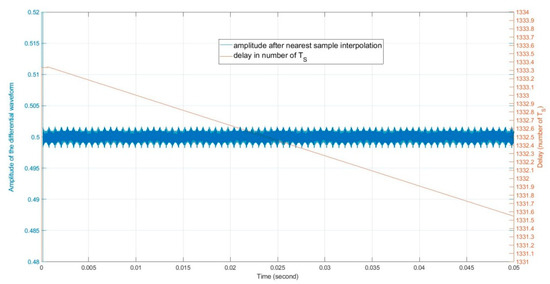
Figure 7. The post nearest sample interpolation waveform amplitude vs. the fractional delay numbers.

2.5. Digital Phased Array

It is assumed that the phased array has $M$ and $N$ elements in X- and Z-direction, respectively, as shown in Figure 8. In our design, the array has uniform element spacing ($d_c$) in both X- and Z-directions. Without loss of generality, it is also assumed $M$ and $N$ are even numbers. Based on the microwave antenna array theory, the array factor in the direction of $\left(\varphi ,\theta \right)$ can be written as the following, if all the elements are uniformly excited with unit amplitude:

$$AF\left(\varphi ,\theta \right)={\displaystyle \sum }_{m=0}^{M-1}{\displaystyle \sum }_{i=0}^{N-1}{e}^{-j \stackrel{\rightharpoonup }{\mathit{K}}\left(\varphi ,\theta \right)·\stackrel{\rightharpoonup }{\mathit{r}}\left(m,i\right)}$$

(8)

where $\stackrel{\rightharpoonup }{\mathit{K}}$($\varphi ,\theta$) is the wave-vector in the direction of $\left(\varphi ,\theta \right)$, and $\stackrel{\rightharpoonup }{\mathit{r}}\left(m,i\right)$ is the displacement from the ${\left(m,i\right)}^{th}$ element to the origin of the coordinate system, they can be expressed as

$$\stackrel{\rightharpoonup }{\mathit{K}}\left(\varphi ,\theta \right)=\frac{2\pi }{\lambda }\left\{\begin{array}{ccc}cos\left(\varphi \right)sin\left(\theta \right) \stackrel{\rightharpoonup }{\mathit{x}},& sin\left(\varphi \right)sin\left(\theta \right) \stackrel{\rightharpoonup }{\mathit{y}},& cos\left(\theta \right)\stackrel{\rightharpoonup }{\mathit{z}}\end{array}\right\}$$

(9)

where λ is the free space wavelength, and

$$\stackrel{\rightharpoonup }{\mathit{r}}\left(m,i\right)=\left\{\begin{array}{cc}x\left(m\right) \stackrel{\rightharpoonup }{\mathit{x}},& 0 \stackrel{\rightharpoonup }{\mathit{y}}, z\left(i\right) \stackrel{\rightharpoonup }{\mathit{z}}\end{array}\right\}$$

(10)

since the array is in the XZ-plane, where $x\left(m\right)=d_c \left(m-\frac{M}{2}+0.5\right)$ and $z\left(i\right)=d_c \left(i-\frac{N}{2}+0.5\right)$. So, Equation (8) can be rewritten as

$$AF\left(\varphi ,\theta \right)={\displaystyle \sum }_{m=0}^{M-1}{\displaystyle \sum }_{i=0}^{N-1}{e}^{-j2\pi \frac{d_c}{\lambda }\left(a\left(0\right)·\left(m-\frac{M}{2}+0.5\right)+a\left(1\right)·\left(i-\frac{N}{2}+0.5\right)\right)}$$

(11)

where

$$\left[a\left(0\right),a\left(1\right)\right]=[cos\left(\varphi \right)sin\left(\theta \right), cos\left(\theta \right)].$$

(12)

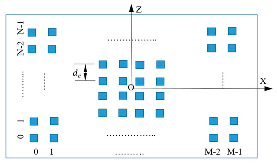
Figure 8. Element locations of the phased array in XZ-plane.

The term of $\left[2\pi \frac{d_c}{\lambda }\left(a\left(0\right)·\left(m-\frac{M}{2}+0.5\right)+a\left(1\right)·\left(i-\frac{N}{2}+0.5\right)\right)\right]$ in Equation (11) can also be considered as the phase needed on the $\left(m,i\right)$^th element in order to let the array form a beam in the $\left(\varphi ,\theta \right)$ direction in digital-domain.

We define the beamforming coefficient of the $\left(m,i\right)$^th element in the array as

$$b_{mi}^c=e^{j2\pi \frac{d_c}{\lambda }\left(a\left(0\right)·\left(m-\frac{M}{2}+0.5\right)+a\left(1\right)·\left(i-\frac{N}{2}+0.5\right)\right)}$$

(13)

3. FMCW Triangular Waveform

The chirp signal uses the triangular waveform. The triangular shape depicts the change of the chirp signal’s frequency component over time. The frequency of transmitted waveform versus time is:

$$f\left(t\right)=\{\begin{array}{cc}{f}_c+2b·\left(mod\left(t,2T\right)-0.5T\right)& \mathrm{for} \mathrm{the} \mathrm{upbeat}\\ f_c+2b·\left(mod\left(2T-t,2T\right)-0.5T\right)& \mathrm{for} \mathrm{the} \mathrm{downbeat}\end{array}$$

(14)

where $f_c$ is the carrier frequency of the chirp signal, and $b$ stands for the slope of the chirp signal, while $T$ stands for the upbeat or downbeat time duration as illustrated in Figure 9.

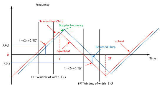
Figure 9. The triangular FMCW waveform.

The transmitted waveform in a closed form is

$$x\left(t\right)=\cos \left(2\pi {{\displaystyle \int }}_0^{t}f\left(\tau \right)d\tau \right)$$

(15)

When this RF signal hits a moving target with the radial speed $v_{tx}\left(t^{\prime }\right)$ (m/s) at a distance $R_{tx}\left(t^{\prime }\right)$ relative to the transmitter, it bounces back to the receiver with the radial speed $v_{rx}\left(t^{\prime }\right)$ (m/s) at a distance $R_{rx}\left(t^{\prime }\right)$ relative to the receiver. The received signal can be expressed in a classical physics sense as:

$$r\left(t\right)=g·\cos \left(2\pi {{\displaystyle \int }}_0^{t-\frac{R_{tx}\left(t^{\prime }\right)+R_{rx}\left(t^{\prime }\right)}{c}}f\left(\tau \right)d\tau +\phi \right)$$

(16)

where $g$ and $\phi$ are the gain and phase introduced by the EM wave reflection/scattering and other losses in the two-way path of TX (antenna)-target-RX (antenna), respectively. $t$ is the time of receiving the signal at the radar receiver, $t=t^{\prime }+\frac{R_{rx}\left(t^{\prime }\right)}{c}$ and $t^{\prime }$ is the time instance that reflection/scattering occurs, and

$$\begin{array}{c}{R}_{tx}\left(t^{\prime }\right)=R_{tx,0}+{{\displaystyle \int }}_0^{t^{\prime }}{v}_{tx}\left(\tau \right)d\tau \\ R_{rx}\left(t^{\prime }\right)=R_{rx,0}+{{\displaystyle \int }}_0^{t^{\prime }}{v}_{rx}\left(\tau \right)d\tau \end{array}$$

(17)

where $R_{tx,0}$ is the initial distance between the transmitter and the target, and $R_{rx,0}$ is the initial distance between the receiver and the target. Note that the observable range for radar measurement is defined as $R\left(t\right)=\frac{R_{tx}\left(t^{\prime }\right)+R_{rx}\left(t^{\prime }\right)}{2},$ and we assume $R\left(t\right)<\frac{cT}{4}$, so that the range ambiguity is not considered.

We choose the FFT windows centered at $t_1$ and $t_2$ as shown in Figure 9 to estimate the Doppler values and ranges with both the upbeat and the downbeat waveform. We assume that the transmitter and the receiver are powered up at the same time, i.e., time $0$, thus $t_1$ and $t_2$ are with respect to this power-up time. In this paper, we choose $t_1=2nT+\frac{2}{3}T$ and $t_2=2nT+\frac{5}{3}T$ as the centers of the FFT windows, and assume that the FFT window has a width of $\frac{T}{3}$. Here, $n$ stands for the $n^{th}$ $2T$ period. With this parameter selection, the guard time is $\frac{T}{2}$ and can guard max one-way propagation time of $\frac{T}{4}$.

By taking derivatives to the phases at $t_1=2nT+\frac{2}{3}T$ and $t_2=2nT+\frac{5}{3}T$ in Equation (16) using the chain rule of derivatives, where $n$ stands for the $n^{th}$ $2T$ period, we can estimate the frequency of the received waveform in the selected FFT windows as:

$$\begin{array}{cc}{f}_u\left(t_1\right)=(f_c+2b& \left(mod\left(t_1,2T\right)-\frac{R_{tx}\left(t_1^{\prime }\right)+R_{rx}\left(t_1^{\prime }\right)}{c}-0.5T\right))\left(1-\frac{\frac{v_{tx}\left(t_1^{\prime }\right)+v_{rx}\left(t_1^{\prime }\right)}{c}}{1+\frac{v_{rx}\left(t_1^{\prime }\right)}{c}}\right)\hfill \\ & =\frac{\left(f_c+2b\left(mod\left(t_1,2T\right)-\frac{R_{tx}\left(t_1^{\prime }\right)+R_{rx}\left(t_1^{\prime }\right)}{c}-0.5T\right)\right)\left(1-\frac{v_{tx}\left(t_1^{\prime }\right)}{c}\right)}{1+\frac{v_{rx}\left(t_1^{\prime }\right)}{c}}\hfill \end{array}$$

(18)

$$\begin{array}{ll}{f}_d\left(t_2\right)& =\left(f_c+2b\left(mod\left(2T-t_2,2T\right)+\frac{R_{tx}\left(t_2^{\prime }\right)+R_{rx}\left(t_2^{\prime }\right)}{c}-0.5T\right)\right)\left(1-\frac{\frac{v_{tx}\left(t_2^{\prime }\right)+v_{rx}\left(t_2^{\prime }\right)}{c}}{1+\frac{v_{rx}\left(t_2^{\prime }\right)}{c}}\right)\\ & =\frac{\left(f_c+2b\left(mod\left(2T - t_2,2T\right)+\frac{R_{tx}\left(t_2^{\prime }\right)+R_{rx}\left(t_2^{\prime }\right)}{c}-0.5T\right)\right)\left(1-\frac{v_{tx}\left(t_2^{\prime }\right)}{c}\right)}{1+\frac{v_{rx}\left(t_2^{\prime }\right)}{c}}\end{array}$$

(19)

The FFT windows centered at $t_1$ and $t_2$ are properly guarded before and after the windows in time so that they only contain the skin return signals in upbeat or downbeat, respectively. This avoids the difficulty in spectrum analysis due to having received signals in both upbeat and downbeat.

We also define the observable radial speed for radar measurement at time $t$ as v$\left(t\right)$, where

$$v\left(t\right)=\frac{v_{tx}\left(t^{\prime }\right)+v_{rx}\left(t^{\prime }\right)}{2\left(1+\frac{v_{rx}\left(t^{\prime }\right)}{c}\right)}.$$

(20)

The quantity $R\left(t\right)$ and $v\left(t\right)$ will be estimated in the simulation. Since the transmitter and the receiver are very close to each other and the speed of the target is much less than the speed of light, we have $v\left(t\right)\approx v_{rx}\left(t^{\prime }\right)\approx v_{tx}\left(t^{\prime }\right).$

Subtracting the frequencies of the transmitted waveforms from $f_u\left(t\right)$ and $f_d\left(t\right),$ we obtain:

$$d_u\left(t_1\right)=-\frac{2f_{c}v\left(t_1\right)}{c}-\frac{4bR\left(t_1\right)}{c}-\frac{4b·\left(mod\left(t_1,2T\right)-0.5T\right)v\left(t_1\right)}{c}+\frac{8bR\left(t_1\right)v\left(t_1\right)}{c^2}$$

(21)

$$d_d\left(t_2\right)=-\frac{2f_{c}v\left(t_2\right)}{c}+\frac{4bR\left(t_2\right)}{c}-\frac{4b·\left(mod\left(2T-t_2,2T\right)-0.5T\right)v\left(t_2\right)}{c}-\frac{8bR\left(t_2\right)v\left(t_2\right)}{c^2}$$

(22)

After plugging in $t_1=2nT+\frac{2}{3}T$ and $t_2=2nT+\frac{5}{3}T$, we obtain:

$$d_u\left(t_1\right)=-\frac{2f_{c}v\left(t_1\right)}{c}-\frac{4bR\left(t_1\right)}{c}-\frac{4bTv\left(t_1\right)}{6c}+\frac{8bR\left(t_1\right)v\left(t_1\right)}{c^2}$$

(23)

$$d_d\left(t_2\right)=-\frac{2f_{c}v\left(t_2\right)}{c}+\frac{4bR\left(t_2\right)}{c}+\frac{4bTv\left(t_2\right)}{6c}-\frac{8bR\left(t_2\right)v\left(t_2\right)}{c^2}$$

(24)

The Doppler frequency is thus estimated by

$$d_{dop}\left(t\right)=-\frac{2f_c{v}_{rx}\left(t\right)}{c}\approx -\frac{2f_{c}v\left(t\right)}{c}\approx (d_u\left(t_1\right)+d_d\left(t_2\right))/2.$$

(25)

By properly choosing the parameters $b$ and $T$, and by ignoring the terms of $\frac{8bR\left(t_1\right)v\left(t_1\right)}{c^2}-\frac{4bTv\left(t_2\right)}{6c}$ and $-\frac{8bR\left(t_2\right)v\left(t_2\right)}{c^2}+\frac{4bTv\left(t_2\right)}{6c}$ since they are very small, as $v\left(t_1\right)$ and $v\left(t_2\right)$ are much smaller than the speed of light $c$, we obtain:

$$R\left(t\right)\approx \frac{R\left(t_1\right)+R\left(t_2\right)}{2}=\frac{\left(d_d\left(t_2\right)-d_u\left(t_1\right)\right)c}{8b}.$$

(26)

4. The Receiver

4.1. The Receiver Diagram

The digital portion of the receiver diagram is shown in Figure 10. It takes complex I/Q samples after ADCs from a 4 × 4 array and filters them with a root-raised-cosine (RRC) filter for each of the ADC input stream. The RX RRC filter is the same as the TX RRC filter. Both RRC filters are used to filter out the out of band spurious signals and to improve the flatness of the in-band frequency domain response. Then de-chirp operations are applied using the baseband version of the TX chirp waveform. After de-chirping, the DC component of each input stream, which retains the TX-to-RX leakage signal, is removed. Then DBF is applied based on angle quantities $a\left(0\right)$ and $a\left(1\right)$. After DBF, 16 signal-streams from vector MTI filter form four partial sums in four quadrants, labeled as A, B, C, and D in Figure 17, for one target. These four signals are sent to four Chebyshev window function units to reduce the sidelobes of the main spurs.

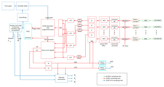
Figure 10. The digital portion of the receiver block diagram.

After the window function, the signals are fed into four FFT engines. Note that the time window of the FFT centers at $t_1$ and $t_2$ specified are shown in Figure 9. These four FFT outputs are added together to form the sum signal after DBF. Note that the four FFT outputs are serialized from FFT index $0$ to FFT index $N_{FFT}-1$ and form four time series at the baseband sampling rate. This is because $N_{FFT}$-point time-domain I/Q signals fed in the FFT and $N_{FFT}$ bins are produced by the FFT engine. Since these FFT indices are proportional to the two-way propagation delays, these time series are called “post-FFT time series”. The pre-FFT time series at the baseband sample rate $f_B$ is indexed by $k$ and the post-FFT time series at the baseband sample rate $f_B$ is indexed by $p$. The key notations are summarized in Table 1.

Table 1. Notations of different indices used in the paper.

Index Name	Definition
$m$	The index of the receive antenna array along the x-axis.
$i$	The index of the receive antenna array along the z-axis.
$k$	The pre-Fast Fourier Transform (FFT) time index at the sample rate of $f_B.$
$p$	The post-FFT time index at the sample rate of $f_B.$
$n$	The time index for the $2T$ time duration intervals.
$I_g$	The post-FFT time index of the range gate center.
$I_{tone}$	The post-FFT time index of the desired tone location of the target.

Tone detection is performed within a specified range gate. The definition of the range gate will be discussed in a later section. The tone location in the post-FFT time series and the range value corresponding to the desired tone’s FFT index are outputted. The error signals $e_0$ and $e_1$ for the measured target are formed based on the tone location and four FFT outputs of the four quadrants A, B, C, and D. Then the PI controller uses these error signals and the initial angle information to form the output angles quantities $a\left(0\right)$ and $a\left(1\right)$. Since the target moves continuously, the range gate needs to be adjusted continuously. This is done by adjusting the delay value of the range gate according to the estimated propagating time based on the range estimates.

4.2. De-Chirp of the Received Signal

The digital version of the transmitted chirp signal from the transmitter is written as $x\left[k\right]$. The output signal from de-chirp signal processing can be expressed as follows:

$$r_{d,mi}\left[k\right]=x^{*}\left[k\right]r_{mi}\left[k\right]$$

(27)

where ${()}^{*}$ is the complex conjugate operation and $r_{mi}\left[k\right]$ is equivalently to $r_{mi}\left(k{T}_B\right)$, which is down-sampled from $r_{mi}\left(k{T}_S\right)$ by a down-sampling factor $K=\frac{f_S}{f_B}$.

As explained in Equation (16), a propagation delay in the round-trip path of the waveform is translated to a frequency shift from the center frequency. By analyzing the de-chirped signal $r_{d,mk}\left[k\right]$ in the baseband, we can see a distinct frequency component, away from the origin of the frequency axis. The amount of frequency shift is in proportion to the signal delay.

4.3. The Vector DC Canceller

It is well known that the useful signal of the target skin return can be buried by the TX-to-RX leakage signal at the receiver with the continuous wave. In some prior arts, the TX-to-RX leakage is attenuated by a DC canceller after the beamforming operation. This imposes some restrictions to the beamforming operation. For example, it requires a stepping response of the angle update for the beamforming operation and requires tight synchronization between the angle update and the DC cancellation. In our design, we use a per antenna DC canceller before the beamforming operation as illustrated in Figure 10 and Figure 11. This is a first order IIR filter. In this manner, the strong DC of the TX-to-RX leakage is removed completely. We illustrate the filter response of the digital DC filter in Figure 12.

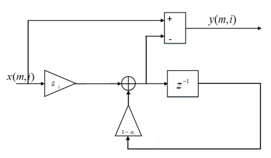
Figure 11. The direct current (DC) canceller for the signal corresponding to the ${\left(m,i\right)}^{th}$ receive antenna, a first order infinite impulse response (IIR) filter, where $a_0=0.0625$.

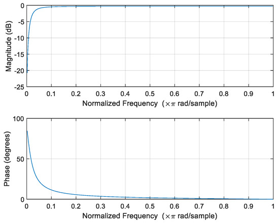
Figure 12. The frequency response of the DC canceller.

Although we can remove the DC component using the DC canceller, relatively weak near DC spurs are in the presence as illustrated later in Figure 18. They are caused due to the non-ideality of the RRC filter. The amplitude response of the RRC filter is not flat. Thus, the FMCW waveform amplitude is modulated by this amplitude response after passing the ideal FMCW waveform through the RRC filter.

4.4. The Vector MTI Filter

In order to remove the effects of the strong echoes of the clutters, an MTI filter is introduced. Since the antenna panel does not move with respect to the ground, the MTI filter can be applied in each receiving channel after each RX antenna before DBF. Normally, the MTI filter can be done in the post-FFT domain. However, it requires per-antenna FFT operations. As illustrated in Figure 10, the FFT operation is after the MTI filters, hence the time domain vector MTI filter is introduced in our design and illustrated in Figure 13. This is because the FMCW waveform is periodic with a period of $\frac{2T}{T_B}$ baseband samples. The MTI filter is FIR and has an order of 4. An IIR version can be introduced to further improve the filter response as a design choice.

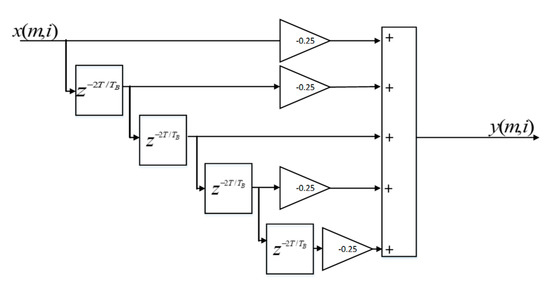
Figure 13. The moving target indication (MTI) filter for the signal corresponding to the ${\left(m,i\right)}^{th}$ receive antenna.

The MTI filter amplitude response versus the target radial speed is shown in Figure 14 as an example. The nulls of the filter correspond to the blind speeds of the target. The first null corresponding to the zero speed can remove the stationary or very low speed clutter echoes from the received signal. The second null corresponding to about 275.5 km/h radial speed is called the blind speed. When the target speed is about an integer multiple of the blind speed, the MTI filter removes the target skin return as well. In the later part of this paper, we introduce the CFAR detector and range extrapolation as a work-around to this issue.

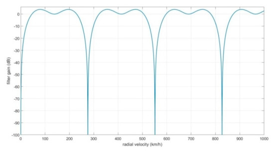
Figure 14. The frequency response of the MTI filter. The blind speed is about 275.5 km/h in this case. The carrier frequency is $f_c=1.5 \mathrm{GHz}$ the baseband sampling rate $f_B=5 \mathrm{MHz}$, and $T=6.528\times {10}^{-4} \mathrm{s}$.

4.5. Range and Doppler Estimation

Let $S_1\left[n\right]$ be the picked tone location from the sum signal in the FFT domain of $\left[0,N_{FFT}-1\right]$ for the $n^{th}$ upbeat, we have:

$$d_u\left[n\right]\approx \frac{(S_1\left[n\right]-N_{FFT})f_B}{N_{FFT}}$$

(28)

Similarly, for the $n^{th}$ downbeat, we can detect a tone at FFT index $S_2\left[n\right]$. We have:

$$d_d\left[n\right]\approx \frac{S_2\left[n\right]f_B}{N_{FFT}}$$

(29)

Based on Equation (26), we can estimate the range as:

$$R\left[n\right]\approx \frac{\left(d_d\left[n\right]-d_u\left[n\right]\right)c}{8b}.$$

(30)

Given the baseband bandwidth $f_B$, the normalized Doppler is defined as:

$$D_{dop}\left[n\right]=\frac{d_{dop}\left[n\right]}{f_B}=-\frac{2f_{c}v\left[n\right]}{c{f}_B}.$$

(31)

Based on Equation (25), we can estimate the normalized Doppler value at the $n^{th}$ FFT window pair (the FFT window for the upbeat and the FFT window for the downbeat) as,

$$D_{dop}\left[n\right]=\frac{d_{dop}\left[n\right]}{f_B}\approx \frac{\left(d_d\left[n\right]+d_u\left[n\right]\right)}{2f_B}.$$

(32)

Note that the estimated range and Doppler are updated at the $1/T$ sampling rate.

4.6. Range Gate

The range gate is denoted by $\left[I_g-G, I_g+G\right],$ where $I_g-G$ and $I_g+G$ lie within the FFT index range of $\left[0,N_{FFT}-1\right],$ and $I_g$ is the center of the range cell under test in either upbeat or downbeat of the echo signal. The tone location $I_{tone}$ of the intended target needs to lie within the range gate. Note that the desired tone index $I_{tone}$ and range gate center index $I_g$ are not always the same. The quantity $G$ allows an uncertainty from the range estimation process and accounts for the sidelobe region in the spectrum due to the window function.

Since the FMCW waveform is modulated, the post-FFT tone is strong in the spectrum main-lobe and it is very weak in the spectrum sidelobe (due to the window function), the conventional range gate control mechanism for the un-modulated signal [4] does not apply. In our design, the gate center control simply uses a moving average filter. The feedback part of the range gate tracking loop consists of “form gate”, “smoothing”, and “variable delay”, as shown in Figure 10. The range gate is first formed using a square waveform generation circuitry with the properly generated gate width $=2G$. Then the range gate tracking loop utilizes a variable delay function, which delays the range gate by the detected FFT tone location index in the post-FFT time series. To improve the tracking accuracy, the FFT tone location indices $S_1\left[n\right]$ and $S_2\left[n\right]$ are smoothed by smoothing $R\left[n\right]$ and $D_{dop}\left[n\right]$. This is the smoothing block illustrated in Figure 10. This moving average tone location is translated into a delay time and is used to delay the range gate accordingly.

4.7. The FMCW CFAR Detector

The standard cell-averaging CFAR detector [26] is applied to the post-FFT domain of the sum signal of DBF as illustrated in Figure 15. From [26], we adopt the CFAR detector figure here for illustration purposes. The cell under test is governed by the range gate of $2G+1$ post-FFT frequency indices centered at $I_g$. In the range cell under test, we pick the index that corresponds to the maximum power of the $2G+1$ frequency indices, i.e., $P_{max}^{tc}.$ Ideally, if the range gate is tracked properly, the center of the test cell corresponds to the maximum. Outside the range cell under test, we collect the average power of the $2G_a$ post-FFT indices to determine the noise and residual clutter power floor, namely, $P_{floor}$. We define $\gamma$ as the power ratio between $P_{max}^{tc}$ and $P_{floor}.$ When $\gamma >{\gamma }_{th}$, the CFAR detector threshold, the index location with the maximum power will be recorded. Otherwise, the location of the maximum will not be discarded.

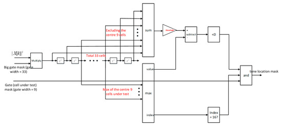
Figure 15. The example of cell-averaging constant false alarm rate (CFAR) detector (credited to [26]), where $G=4$, $G_a=12,$ and $threshold=\frac{{\gamma }_{th}}{2G_a}$. The tone location masks will be further classified as upbeat tone location masks and downbeat tone location masks as shown in Figure 20.

If this tone location $I_{tone}$ is recorded, the mono-pulse “Form error signals” in Figure 10 is activated at this tone location of the post-FFT time series. The mono-pulse error signals are then enabled and are fed into the PI controller. More on mono-pulse error signals will be given later. Otherwise, the mono-pulse angle tracking follows the angle memory stored in the PI controller in Figure 16 in the current time duration interval of $T$.

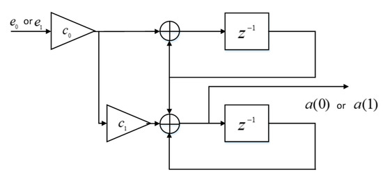
Figure 16. PI controller. Input is the error signal and output is the estimate of angle tracking quantities.

4.8. Range Extrapolation Using Doppler Estimate for Low Signal-to-Noise Ratio (SNR)

When the strength of the signal tone is below the CFAR detection threshold, we use a scheme to extrapolate the range estimation based on the last known range estimate $R[n_{last}]$ and last known Doppler estimate $d_{dop}\left[n_{last}\right]$. Since the signal tone can be significantly attenuated when the radial velocity is close to the integer multiple of the MTI blind speed, under this situation, the range extrapolation scheme helps to follow the actual range. The extrapolation uses the following simple formula:

$$R\left[n\right]=R\left[n_{last}\right]-\frac{D_{dop}\left[n_{last}\right]c{f}_B}{2f_c}\left(n-n_{last}\right)2T.$$

(33)

The range extrapolation can be effective only when the last known range and Doppler estimation are relatively accurate.

4.9. Four-Quadrant Digital Mono-Pulse Tracking

The four-quadrant mono-pulse tracking algorithm for pulse Doppler radar with mechanical steering can be found in [28]. Here, we extend this algorithm to the FMCW phased array angle tracking scenario. The antenna panel is equally divided into four quadrants, labeled as A, B, C, and D, as illustrated in Figure 17. The partial sum of received signals after digital beam forming in the quadrant $q=A, B, C or D$ has the following form:

$$y_q\left[k\right]={\displaystyle \sum }_{\left\{m,i within quadrant q\right\}}{r}_{d,mi}\left[k\right]·b_{mi}^c$$

(34)

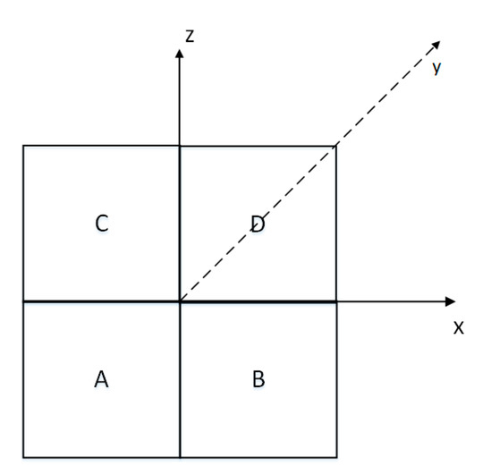
Figure 17. Four quadrants on the antenna plane, note that the view direction is from the receiver to the target, i.e., Y-direction points into the paper.

After the $N_{FFT}$ point FFT, the output from each quadrant is $Y_q\left[p\right]$, where $p$ is the post-FFT time-series index. If target tone locations from CFAR detection are recorded in the upbeat and downbeat of the $n^{th}$ FFT window pair during the $n^{th}$ 2T time-period, the signal of these tones can be represented as $Y_q^u\left[n\right]$ and $Y_q^d\left[n\right]$, respectively. The sum signal is $Y\left[p\right]={{\displaystyle \sum }}_q{Y}_q\left[p\right]$. For the upbeat and downbeat of the $n^{th}$ FFT pair, the CFAR detected sum signals are $Y^u\left[n\right]={{\displaystyle \sum }}_q{Y}_q^u\left[n\right]$ and $Y^d\left[n\right]={{\displaystyle \sum }}_q{Y}_q^d\left[n\right]$.

4.10. Angle Tracking Error Signals

The tone location $I_{tone}$ in the post-FFT time series will be used to read the FFT outputs from the A, B, C, and D quadrants, denoted by $Y_A\left[I_{tone}\right]$, $Y_B\left[I_{tone}\right]$, $Y_C\left[I_{tone}\right],$ and $Y_D\left[I_{tone}\right]$. Then we can form the angle tracking error signals $e_0$ and $e_1$ as follows,

$$e_0=-\angle \left(\left(Y_B\left[I_{tone}\right]+Y_D\left[I_{tone}\right]\right){\left(Y_A\left[I_{tone}\right]+Y_C\left[I_{tone}\right]\right)}^{*}\right)$$

(35)

$$e_1=-\angle \left(\left(Y_C\left[I_{tone}\right]+Y_D\left[I_{tone}\right]\right){\left(Y_A\left[I_{tone}\right]+Y_B\left[I_{tone}\right]\right)}^{*}\right),$$

(36)

where $\angle$ stands for evaluating the angle of a complex number.

4.11. Angle Tracking Loop

The angle tracking loop relies on a closed loop control feedback mechanism. The classical PI controller is used to drive the digital beamformer. Starting from the initial $a\left(0\right)$ and $a\left(1\right)$ values in the proximity of true $a\left(0\right)$ and $a\left(1\right),$ the controller uses $e_0$ and $e_1$ to update the new estimated $a\left(0\right)$ and $a\left(1\right)$ values for the digital beamformer. The new estimated $a\left(0\right)$ and $a\left(1\right)$ will affect the estimation of the new $e_0$ and $e_1$ values.

The PI controller implementation in the baseband sampling domain has the structure shown in Figure 16.

The constant value $c_0=0.0188$. The constant $c_1=\frac{1}{256}.$ $c_0$ and $c_1$ are fine-tuned for a medium range scenario. They can be scaled by the inverses of the estimated range values.

4.12. Velocity Estimation

Based on two range and angle estimations separated by $dd·2T$ time duration, we can estimate the velocity on the $x, y, z$ axes

$$\begin{array}{l}{v}_x\left[n\right]=\frac{x\left[n\right]-x\left[n+dd\right]}{dd·2T}\\ v_y\left[n\right]=\frac{y\left[n\right]-y\left[n+dd\right]}{dd·2T}\\ v_z\left[n\right]=\frac{z\left[n\right]-z\left[n+dd\right]}{dd·2T}\end{array}$$

(37)

where $n$ denotes the $n^{th}$ $2T$ time period, and

$$\begin{array}{c}x\left[n\right]=R\left[n\right]·cos\left(\varphi \left[n\right]\right)·sin\left(\theta \left[n\right]\right)\\ y\left[n\right]=R\left[n\right]·sin\left(\varphi \left[n\right]\right)·sin\left(\theta \left[n\right]\right)\\ z\left[n\right]=R\left[n\right]·cos\left(\theta \left[n\right]\right).\end{array}$$

(38)

5. Results

In this section, we present the Simulink simulation results. The simulation setup is first presented. Then, in this controlled environment, we compare the angle, range, Doppler, and velocity estimation results of three configured scenarios with the true angle, range, Doppler, and velocity values.

5.1. Simulation Setup

We first simulate the effect of line-of-sight target skin return to lower the computational complexity in order to demonstrate a fully functional FMCW-based moving target tracking and measurement system. Then, we focus on the results in the scenario with a target, where it is fast moving and a strong clutter with zero velocity. Additionally, for simplicity, the simulation considers none of the effects of target glint, angle scintillation, atmospheric propagation, and multi-path propagation. The Simulink parameters are shown in Table 2.

Table 2. Common simulation parameters.

Variable Name	Value	Definition
$M$	$4$	Number of receive antenna elements on the x axis.
$N$	$4$	Number of receive antenna elements on the z axis.
$h_0^c$	$exp\left(1i·rand\right)$	Phases of the channel of the target skin return, $1i=\sqrt{-1}$ and rand is the uniform random number generator.
$\left({\varphi }_{\mathrm{R}},{\theta }_{\mathrm{R}}\right)$	$\left(\frac{\pi }{2},\frac{\pi }{2}\right)$	The initial azimuth and elevation angle for the RX beam.
$aa0$	$variable$	The initial azimuth angle of the moving target.
$taa0$	$variable$	The initial value of the azimuth tracking angle.
$ae0$	$variable$	The initial elevation angle of the moving target.
$tae0$	$variable$	The initial value of the elevation tracking angle.
$R_{rx,0}$	$variable$	The initial distance between the receiver and the target. Additionally, it is the range corresponding to the center of the initial range bin.
$d_{TR}$	$3 \mathrm{m}$	The distance between the transmitter and the receiver phase reference centers.
${\sigma }_0$	$17 {\mathrm{dBm}}^2$	Radar cross section (RCS) of the target.
$h_1^c$	$exp\left(1i·rand\right)$	Phases of the channel of the clutter skin return.
$aa1$	$variable$	The azimuth angle of the clutter.
$ae1$	$variable$	The elevation angle of the clutter.
$R_1$	$variable$	The distance between the tracking and measurement system and the clutter.
${\sigma }_1$	$37 {\mathrm{dBm}}^2$	RCS of the clutter.
$f_c$	$1.5 \mathrm{GHz}$	The carrier frequency of the tracking and measurement system.
$f_B$	$5 \mathrm{MHz}$	The baseband sampling rate.
$f_s$	$2f_B$	Oversampling rate.
$v$	$variable$	Target velocity towards the tracking and measurement system on the x, y, z axes.
$accel$	$\left[0 0 0\right] \mathrm{m}/{\mathrm{s}}^2$	Velocity acceleration of each target towards the tracking and measurement system on the x, y, z axes.
$T$	$6.528\times {10}^{-4} \mathrm{s}$	The upbeat or downbeat duration.
$b$	$3.0637 \mathrm{GHz}/\mathrm{s}$	Chirp signal slope.
$G_{tR,t}$	$variable,$ $dependent on$ $the angles of$ $the moving$ $target$	The TX antenna gain for the target assuming a uniform beam pattern on the azimuth and a very narrow beam pattern on the elevation. The gain on the azimuth plane is $21.46 \mathrm{dBi}$ uniformly. The main-lobe of the TX antenna always points to the moving target.
$G_{tR,c}$	$variable,$ $dependent on$ $the angles of$ $the clutter$	The TX antenna gain for the clutter assuming a uniform beam pattern on the azimuth and a very narrow beam pattern on the elevation. The gain on the azimuth plane is $21.46 \mathrm{dBi}$ uniformly.
$G_{rR}$	$0 \mathrm{dBi}$	The RX antenna gain assuming an omnidirectional receive antenna pattern.
$d_c/\lambda$	$0.5$	The ratio of antenna spacing and wavelength.
$P_t$	$62 \mathrm{dBm}$	The transmit power.
$noise\_fl$	$-166 \mathrm{dBm}/\mathrm{Hz}$	The noise floor at $290 \mathrm{kelvin}$ temperature and including the noise figure of $8 \mathrm{dB}$.
$rrcord$	$32$	Root raised cosine pulse shaping filter order in the baseband sampling rate. This filter is applied to the transmitter.
$rrcord1$	$32$	Root raised cosine pulse shaping filter order in the baseband sampling rate. This filter is applied to the receiver.
$lagord$	$8$	Lagrange filter order in the oversampling domain.
$lpwr$	$-18 \mathrm{dBm}$	TX to RX leakage power between the transmitter and each receive antenna.
$N_{FFT}$	$1024$	Number of FFT points.
$I_{avg0}$	$0$	Range IIR smoothing filter order, the filter response looks like $\frac{0.25}{1-0.75z^{-1}}$, where z-transform is with respect to the sampling rate of $1/T$.
$M_{avg1}$	$15$	Doppler moving average filter order, the filter response looks like ${{\displaystyle \sum }}_{pp=0}^{15}\frac{z^{-pp}}{16}$, where z-transform is with respect to the sampling rate of $1/T$.

Note that the quantities like initial angles and initial ranges of the moving target and the clutter are variables changing based on the scenarios. This table shows the common parameters used for the simulation scenarios. We will define the three scenarios later. In each scenario, we apply the standard Chebyshev window with $80 \mathrm{dB}$ sidelobe suppression.

With the $1024$ point FFT, the resolution range of the radar in the frequency domain $=0.25·c·\mathrm{sweep} \mathrm{time} \mathrm{for} \mathrm{one} \mathrm{FFT} \mathrm{index}=0.25·c·(f_B/nfft/2b)=59.8 \mathrm{m}$. The range gate spans $9$ frequency indices. The guard range of the range gate is translated from the guard frequency indices from the left or the right of the center frequency index in the range gate, and it is equal to $538 \mathrm{m}.$ Due to the blind speed effect, the target tone is fully buried under the noise floor for a certain period of time, and even when the target moves out of the blind speed, the target tone is no longer at the center of the range gate. There exists a range offset between the times before and after the blind speed zone when the target is detected. Therefore, we need a wider range gate to accommodate this range offset so that the target tone can be re-detected when the target moves out of the blind speed.

The radar operates at $1.5 \mathrm{GHz}$ carrier frequency. The triangular chirp signal has a period of $6528 T_B$ samples. The blind speed is 275.5 km/h.

There are three simulation scenarios. Scenario I and II are used to demonstrate both the CFAR detector and the range extrapolation functions. Scenario III is used to demonstrate how the long range and high-speed tracking work.

The initial range and angle and the TX antenna gain information are common for the scenarios I and II. They are shown in Table 3. The initial range of the moving target is $20 \mathrm{km}$. The mean square of the velocity vector of the moving target is $3402 \mathrm{km}/\mathrm{h}$, equivalently $2.74 \mathrm{Mach}$. The initial radial speed is about $1966 \mathrm{km}/\mathrm{h}$, i.e., $7.14·blind speed$. The target moves into the blind speed Doppler zone, then moves out of it in these scenarios. In the scenario I, we set the CFAR detector threshold $=10 \mathrm{dB}$ and turn off the range extrapolation. In the scenario II, we set the CFAR detector threshold $=14.77 \mathrm{dB}$ and turn off the range extrapolation. We also illustrate the matching of the SNR measurement and the SNR calculation in the simulations. We also illustrate the CFAR detector works with its detection diagram over time.

Table 3. Simulation parameters for Scenario I and II.

Variable Name	Value	Definition
$aa0$	$1.2490 \mathrm{radian}$	The initial azimuth angle of the moving target.
$taa0$	$1.2566 \mathrm{radian}$	The initial value of the azimuth tracking angle.
$ae0$	$1.6332 \mathrm{radian}$	The initial elevation angle of the moving target.
$tae0$	$1.6406 \mathrm{radian}$	The initial value of the elevation tracking angle.
$R_{rx,0}$	$20 \mathrm{km}$	The initial distance between the receiver and the target. Additionally, it is the range corresponding to the center of the initial range bin.
$aa1$	$1.2490 \mathrm{radian}$	The azimuth angle of the clutter.
$ae1$	$1.5084 \mathrm{radian}$	The elevation angle of the clutter.
$R_1$	$19.5 \mathrm{km}$	The distance between the tracking and measurement system and the clutter.
$v$	$\left[3250,1000,100\right]$	Target velocity towards the tracking and measurement system on the x, y, z axes.
$G_{tR,t}$	$21.46 \mathrm{dB}$	The TX antenna gain for the target assuming a uniform beam pattern on the azimuth and a very narrow beam pattern on the elevation. The gain on the azimuth plane is $21.46 \mathrm{dBi}$ uniformly. The mainlobe of the TX antenna always points to the moving target.
$G_{tR,c}$	$17.83 \mathrm{dB}$	The TX antenna gain for the clutter assuming a uniform beam pattern on the azimuth and a very narrow beam pattern on the elevation.

Scenario III is a long-range and high-speed target scenario. The parameters like initial range and angle information are shown in Table 4. The initial range of the moving target is $40 \mathrm{km}$. The mean square of the velocity vector of the moving target is $7360 \mathrm{km}/\mathrm{h}$, equivalently $5.93 \mathrm{Mach}$. The initial radial speed is about $3657 \mathrm{km}/\mathrm{h}$, i.e., $13.28·blind speed.$ The target moves into the blind speed Doppler zone, then moves out of it in this scenario. Due to relatively low SNR in Scenario III, we just set the CFAR detector threshold $=10 \mathrm{dB}$ and turn on the range extrapolation.

Table 4. Simulation parameters for Scenario III.

Variable Name	Value	Definition
$aa0$	$1.3258 \mathrm{radian}$	The initial azimuth angle of the moving target.
$taa0$	$1.3265 \mathrm{radian}$	The initial value of the azimuth tracking angle.
$ae0$	$\pi /2 \mathrm{radian}$	The initial elevation angle of the moving target.
$tae0$	$\pi /2 \mathrm{radian}$	The initial value of the elevation tracking angle.
$R_{rx,0}$	$40 \mathrm{km}$	The initial distance between the receiver and the target. Additionally, it is the range corresponding to the center of the initial range bin.
$aa1$	$0.9828 \mathrm{radian}$	The azimuth angle of the clutter.
$ae1$	$\pi /2 \mathrm{radian}$	The elevation angle of the clutter.
$R_1$	$39 \mathrm{km}$	The distance between the tracking and measurement system and the clutter.
$v$	$\left[7080,2000,200\right]$	Target velocity towards the tracking and measurement system on the x, y, z axes.
$G_{tR,t}$	$21.46 \mathrm{dB}$	The TX antenna gain for the target assuming a uniform beam pattern on the azimuth and a very narrow beam pattern on the elevation. The gain on the azimuth plane is $21.46 \mathrm{dBi}$ uniformly. The mainlobe of the TX antenna always points to the moving target.
$G_{tR,c}$	$21.46 \mathrm{dB}$	The TX antenna gain for the clutter assuming a uniform beam pattern on the azimuth and a very narrow beam pattern on the elevation. The gain on the azimuth plane is $21.46 \mathrm{dBi}$ uniformly.

5.2. Simulation Results

5.2.1. Unit Test for the Vector MTI Filter

The spectrum plot at $0.009 \mathrm{s}$ of the simulation with the vector MTI filter turned off is shown in Figure 18. The simulation setup is using scenario II. The post beamforming noise floor in the simulation is normalized to $0 \mathrm{dBm}$ (equivalent to $1 \mathrm{mW}$) with a gain normalization. This gain is introduced at the receiver and the signal power is scaled accordingly. Based on Table 2, the noise floor is $-166$ dBm/Hz at each receiver antenna. The baseband bandwidth is 5 MHz. The noise power after DBF combining of 16 elements is $-88.22 \mathrm{dBm}$. Normalization is done by introducing a gain of $88.22 \mathrm{dB}$.

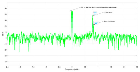
Figure 18. The spectrum plot in one FFT window at $0.009 \mathrm{s}$ of the simulation without the MTI.

For the spectrum plot, since we apply the Chebyshev window for the spectrum analysis, additionally, the Chebyshev window enhances the noise floor by $1.81 \mathrm{dB}$. Based on Equation (1) (the radar range equation), adding the normalization gain of $88.22 \mathrm{dB}$, the DBF gain of $12.04 \mathrm{dB}$ and the FFT gain of $30.10 \mathrm{dB}$, the signal power of the target after the FFT and the DBF is $22.62 \mathrm{dBm}$. The measured signal power of the target tone is $22.68 \mathrm{dBm}.$ The difference is small. The actual SNR of the target is $20.81 \mathrm{dB}$. Similarly, the signal power of the clutter after the FFT and the DBF is $38.95 \mathrm{dBm}$ based on the calculation. The measured signal power of the clutter spur is $38.23 \mathrm{dBm}$. The difference is caused by the signal leakage that happens when the exact spur location in the frequency domain does not align with the FFT index grid.

The spectrum plot at the end of the $0.914 \mathrm{s}$ simulation with the vector MTI filter turned on is shown in Figure 19. In this case, the noise floor is $0.97 \mathrm{dBm}$ because the MTI filter enhances the noise power by $1.25$ times, which is the summation of the squares of the filter coefficients $\left[-0.25,-0.25, 1,-0.25,-0.25\right]$. Additionally, the Chebyshev window enhances the noise floor by $1.81 \mathrm{dB}$. Compared with the Figure 18, the clutter spur and the two near DC spurs are both removed by the MTI filter. The measured signal power of the target tone is $25.03 \mathrm{dBm}$. Given the final normalized Doppler value of 0.001037 and the chirp period of $6528 T_B$ samples, the MTI filter gain is calculated as $3.07 \mathrm{dB}$. Additionally, the final range reading is $19.51 \mathrm{km}$. Therefore, the calculated signal power is $26.18 \mathrm{dBm},$ where the initial signal power is $22.68 \mathrm{dBm}$ at the $20 \mathrm{km}$ range. The difference between the measured and calculated signal powers of the target tone is likely caused by the angle error and the signal leakage due to the misalignment of the tone location with the FFT index grid. The SNR of the target tone is actually equal to $22.40 \mathrm{dB}$.

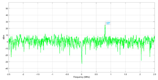
Figure 19. The spectrum plot in the FFT window at $0.914 \mathrm{s}$ in the scenario II with the MTI.

5.2.2. Unit Test for the CFAR Detector

For scenario II, we plot the unit test results for the CFAR detector. In Figure 20, we plot the mask values of the tone locations, the mask values of the range gates, and the SNRs in dB scale. The mask takes a Boolean value of 1 or 0, representing whether or not the tone is detected in the second sub-figure or whether or not the range gate is selected in the first sub-figure. We observe that the CFAR detector cannot detect any tone location when the SNR is lower than $11 \mathrm{dB}$. Note that in this scenario, the CFAR detector threshold is $14.77 \mathrm{dB}$. This means that the cut-off of the successful detection does not happen at $14.77 \mathrm{dB}$, but lower than $14.77 \mathrm{dB}$. The main reason is that in CFAR detector, the cell averaging noise floor estimator uses only 24 cells, hence the noise floor estimation can be underestimated. In Figure 21, we zoom in the plot of the CFAR detection time diagram. The tone locations in upbeat and downbeat are at the centers of the range gates, respectively.

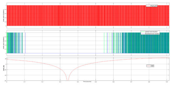
Figure 20. The time diagram of tone location detection vs. SNR at the CFAR detector. The SNR is plotted in dB scale. The values of tone location masks and the range gate are Booleans.

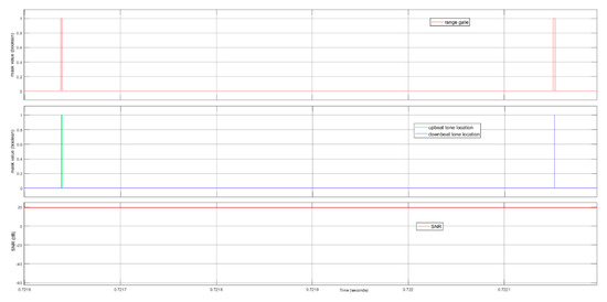
Figure 21. The zoom-in time diagram of tone location detection vs. SNR at the CFAR detector. The tone locations are located at the centers of the range gate in two time instances. The SNR is plotted in dB scale. The values of tone location masks and the range gate are Booleans.

5.2.3. Angle Estimation

In Figure 22, the estimated angle values in Scenario I and Scenario II are compared against the true angle values in terms of $a\left(0\right)$ and $a\left(1\right)$. Due to the blind speed effect, in Scenario I, there is about $0.4 \mathrm{s}$ of time during which the intended tone has a low SNR, which is below or close to the CFAR detector threshold of 10 dB. The low CFAR detector threshold value causes a larger tracking error during this period of time than the result of Scenario II. In Scenario II, there is also about $0.4 \mathrm{s}$ of time during which the intended tone has a low SNR below the CFAR detector threshold of $14.77 \mathrm{dB}$. In this case, the angle tracking is purely driven by the memory of the PI controller. When the radial speed is not close to an integer multiple of the blind speed, the tracking error is smaller than $0.01 \mathrm{radian}$ ($0.57 \mathrm{degree}$).

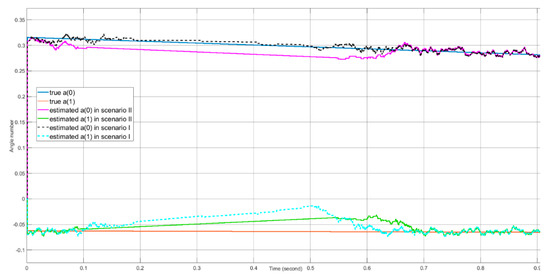
Figure 22. The angle estimation results for Scenario I and Scenario II.

In Figure 23, the estimated angle values in Scenario III are compared against the true $a\left(0\right)$ and $a\left(1\right).$ During the 0.4 s of time when the SNR is below the CFAR detector threshold, the angle tracking is driven by the memory of the PI controller and occasional false alarms. When the target is out of the blind speed Doppler zone, the tracking error is smaller than $0.025 \mathrm{radian}$ ($1.43 \mathrm{degree}$).

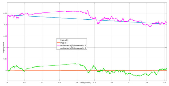
Figure 23. The angle estimation results for Scenario III.

5.2.4. Range Estimation

We plot the range estimate versus the true distance between the receiver (the origin of the coordinate system) and the target $R_{rx}$ in Figure 24 and Figure 25. In Figure 24, due to the higher CFAR detector threshold and the range extrapolation scheme in Scenario II, the range tracking error in Scenario II is much smaller than that of Scenario I during the “blind speed” period of about 0.4 s. During rest of the time, the tracking errors of the two scenarios are similar to each other. In Figure 25, the maximum range estimation error of Scenario III is lower than $200 \mathrm{m}$ during the blind speed Doppler zone of $0.4 \mathrm{s}$ time.

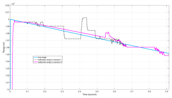
Figure 24. The range estimation results for Scenario I and Scenario II.

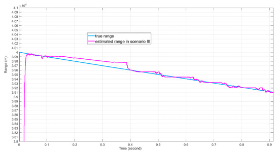
Figure 25. The range estimation results for Scenario III.

5.2.5. Doppler Estimation

The Doppler tracking results are presented in Figure 26 and Figure 27. In Figure 26, during the “blind speed” period, the estimated Doppler value fluctuates more often in Scenario I than the estimated value in Scenario II due to the lower CFAR detector threshold value in Scenario I. The normalized Doppler tracking error is smaller than 0.002. The Doppler tracking error is thus smaller than 10,000 HZ. In Figure 27, the Doppler tracking error of Scenario III is also lower than 10,000 HZ.

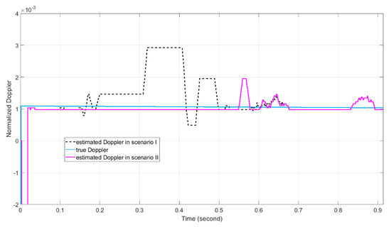
Figure 26. The Doppler estimation results for Scenario I and Scenario II.

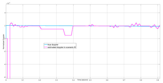
Figure 27. The Doppler estimation results for Scenario III.

5.2.6. Velocity Estimation

The velocity tracking results are presented in Figure 28 and Figure 29. The estimated velocities the in $x$, $y,$ and $z$ axes during the “blind speed” period are not in agreement with the true velocities for all three scenarios, mainly due to the angle tracking error in the blind speed Doppler zone.

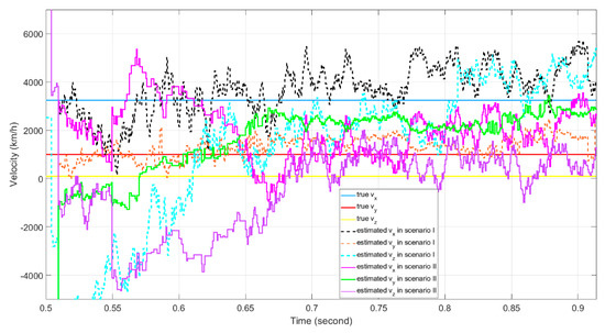
Figure 28. The velocity estimation results for Scenario I and Scenario II.

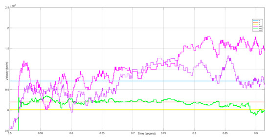
Figure 29. The velocity estimation results for Scenario III.

5.2.7. The RMS Errors When Normal Tracking Takes Place

From the angle, range, Doppler, and velocity plots, both scenario I and II have the common normal tracking period beyond $0.5 \mathrm{s}$ of simulation time. Normal tracking simply means that the SNR values in each scenario after the MTI filter are above each of the CFAR detector thresholds of each scenario. Since all random generators for noise use the same random seeds, the simulation results are roughly the same after $0.5 \mathrm{s}$ of simulation time. The calculated RMS errors are shown in Table 5.

Table 5. RMS errors when normal tracking takes place.

Performance Indicator	RMS Tracking Error
	Scenario I	Scenario II	Scenario III
$a\left(0\right)$	$0.0044 \mathrm{radian}$	$0.0056 \mathrm{radian}$	$0.0069 \mathrm{radian}$
$a\left(1\right)$	$0.0062 \mathrm{radian}$	$0.0066 \mathrm{radian}$	$0.0118 \mathrm{radian}$
Range	$26 \mathrm{m}$	$34 \mathrm{m}$	$26 \mathrm{m}$
Normalized Doppler	$0.00019$ ($950 \mathrm{Hz}$)	$0.000175$ ($875 \mathrm{Hz}$)	$0.00022$ ($1100 \mathrm{Hz}$)

5.2.8. The Total Simulation Time

The total recorded simulation time is roughly $5000 \mathrm{s}$ for $0.914 \mathrm{s}$ of real time simulation. To speed up the simulation and the processing, the proposed hybrid time and frequency domain signal processing with target moving scenario will be planted on a commercial FPGA board, so that much faster M&S can be achieved.

6. Discussion

The simulation results presented in Section 5 agree with the theoretical predictions given by different CFAR detector threshold values. On the other hand, the hybrid time-domain and frequency-domain processing design has lower complexity than the per antenna FFT design. The number of FFT engines used is $4$ instead of $16$ for the case of $16$ antenna. In future work, we would like to build a moving target tracking and measurement test bed with the presented receiver processing unit to collect some experimental data. This testbed will be set up when the FPGA implementation, the RF frontend, and the antenna system are ready.

7. Conclusions

The system model of a digital beamforming phased array system for fast moving object skin-return signal processing is presented in this paper with numerical modeling in Simulink. Using FMCW modulated EM wave, the proposed array system interrogates a moving target in a clutter environment and measures object in range, angle, and Doppler using joint time and frequency domain signal processing. Comparing with existing FMCW based tracking systems, the new system has much lower complexity, especially for a DBF array with large number of elements. Even at $40 \mathrm{km}$ range and $5.93 \mathrm{Mach}$ radial-speed, simulation results show that the system root-mean-square errors of range, angle, and Doppler tracking are $26 \mathrm{m}$, $0.68 \mathrm{degree},$ and $1100 \mathrm{Hz}$, respectively. To speed up the simulation and the design process, the proposed hybrid time and frequency domain signal processing with target moving scenario will be planted on a commercial FPGA board. This way, much faster M&S can be achieved. In addition, the actual baseband processing chain on FPGA would allow real measurements in field experiments.

References

- Melvin, W.L.; Scheer, J.A. Principles of Modern Radar: Radar Applications; Scitech Publishing: Chennai, India, 2014. [Google Scholar]
- Stove, A.G. Linear FMCW radar techniques. IEE Proc. F Radar Signal Process. 1992, 139, 343. [Google Scholar] [CrossRef]
- Hawkins, L.; Walsh, P.; Liner, J.; Curtin, M.; Mullins, M. Radar, Defense vs. Automotives. Available online: https://www.microwavejournal.com/ext/resources/files/EuMW2013DefenseForum/ADI--EuMW-Radar-Defence-Security-Forum.pdf?1522101970 (accessed on 22 December 2020).
- Filippo, N. Introduction to Electronic Defense Systems, 2nd ed.; Artech House: London, UK, 2011. [Google Scholar]
- Rohling, H.; Möller, C. Radar Waveform for Automotive Radar Systems and Applications. In Proceedings of the 2008 IEEE Radar Conference, Rome, Italy, 26–28 May 2008; pp. 1–4. [Google Scholar]
- Choi, J.; Park, J.; Yeom, D. High Angular Resolution Estimation Methods for Vehicle FMCW Radar. In Proceedings of the 2011 IEEE CIE International Conference on Radar, Chengdu, China, 24–27 October 2011. [Google Scholar]
- Su, L.; Wu, H.S.; Tzuang, C.K.C. 2D FFT and Time-Frequency Analysis Techniques for Multi-Target Recognition of FMCW Radar Signal. In Proceedings of the Asia-Pacific Microwave Conference 2011, Melbourne, Australia, 5–8 December 2011. [Google Scholar]
- Dudek, M.; Nasr, I.; Bozsik, G.; Hamouda, M.; Kissinger, D.; Fischer, G. System Analysis of a Phased-Array Radar Applying Adaptive Beam-Control for Future Automotive Safety Applications. IEEE Trans. Veh. Technol. 2015, 64, 34–47. [Google Scholar] [CrossRef]
- Kim, S.; Oh, D.; Lee, J. Joint DFT-ESPRIT Estimation for TOA and DOA in Vehicle FMCW Radars. IEEE Antennas Wirel. Propag. Lett. 2015, 14, 1710–1713. [Google Scholar] [CrossRef]
- Lin, J.-J.; Li, Y.-P.; Hsu, W.-C.; Lee, T.-S. Design of an FMCW radar baseband signal processing system for automotive application. SpringerPlus 2016, 5, 1–16. [Google Scholar] [CrossRef] [PubMed]
- Hyun, E.; Jin, Y.-S.; Lee, J. Design and Implementation of 24 GHz Multichannel FMCW Surveillance Radar with a Software-Reconfigurable Baseband. J. Sens. 2017, 2017, 1–11. [Google Scholar] [CrossRef]
- Saponara, S.; Neri, B. Radar Sensor Signal Acquisition and Multidimensional FFT Processing for Surveillance Applications in Transport Systems. IEEE Trans. Instrum. Meas. 2017, 66, 604–615. [Google Scholar] [CrossRef]
- Jin, Y.; Kim, B.; Kim, S.; Lee, J. Design and Implementation of FMCW Surveillance Radar Based on Dual Chirps. Elektron. Elektrotechnika 2018, 24, 60–66. [Google Scholar] [CrossRef]
- Hyun, E.; Jin, Y.-S.; Ju, Y.; Lee, J.-H. Development of Short-Range Ground Surveillance Radar for Moving Target Detection. In Proceedings of the 2015 IEEE 5th Asia-Pacific Conference on Synthetic Aperture Radar (APSAR ‘15), Singapore, 1–4 September 2015; pp. 692–695. [Google Scholar]
- Kim, B.; Jin, Y.-S.; Kim, S.; Lee, J. A Low-Complexity FMCW Surveillance Radar Algorithm Using Two Random Beat Signals. Sensors 2019, 19, 608. [Google Scholar] [CrossRef] [PubMed]
- Lischi, S.; Massini, R.; Musetti, L.; Staglianò, D.; Berizzi, F.; Neri, B.; Saponara, S. Low Cost FMCW Radar Design and Implementation for Harbour Surveillance Applications. In Applications in Electronics Pervading Industry, Environment and Society; Springer: New York, NY, USA, 2015; pp. 139–144. [Google Scholar]
- System Tool Kit (STK) Description; Analytical Graphics, Inc.: Exton, PA, USA, 2019; Available online: www.agi.com (accessed on 22 December 2020).
- Skolnik, M. Radar Handbook, 2nd ed.; McGraw-Hill: New York, NY, USA, 1990. [Google Scholar]
- Wu, C.; Navarro, A.; Litva, J. Combination of finite impulse response neural network technique with FDTD method for simulation of electromagnetic problems. Electron. Lett. 1996, 32, 1112. [Google Scholar] [CrossRef]
- Wu, C.; Navarro, E.A.; Navasquillo, J.; Litva, J. FDTD signal extrapolation using a finite impulse response neural network model. Microw. Opt. Technol. Lett. 1999, 21, 325–330. [Google Scholar] [CrossRef]
- Chen, V.C.; Li, F.; Ho, S.S.; Wechsler, H. Micro-Doppler Effect in Radar Phenomenon, Model, and Simulation Study. In IEEE Transactions on Aerospace and Electronic Systems; IEEE: Piscataway, NJ, USA, 2006; Volume 42. [Google Scholar]
- Proakis, J.G. Digital Communications, 3rd ed.; McGraw-Hill: New York, NY, USA, 1995. [Google Scholar]
- Tang, T.; Wu, C. Design of New FMCW Target Tracking Radar with Digital Beamforming Tracking; DRDC Scientific Report, DRDC-RDDC-2019-R175; Defence Research and Development Canada: Ottawa, ON, Canada, 2019.
- Ash, M.; Ritchie, M.; Chetty, K. On the Application of Digital Moving Target Indication Techniques to Short-Range FMCW Radar Data. IEEE Sens. J. 2018, 18, 4167–4175. [Google Scholar] [CrossRef]
- Miller, R. Fundamentals of Radar Signal Processing; McGraw-Hill: New York, NY, USA, 2005. [Google Scholar]
- Finn, H.M.; Johnson, R.S. Adaptive Detection Mode with Threshold Control as a Function of Spatially Sampled Clutter-level Estimates. RCA Rev. 1968, 29, 141–464. [Google Scholar]
- Rhodes, D.R. Introduction to Monopulse; McGraw-Hill: New York, NY, USA, 1959. [Google Scholar]
- Shernman, S.M.; Barton, D.K. Monopulse Principles and Techniques, 2nd ed.; Artech House: London, UK, 2011. [Google Scholar]
- Stone, L.D.; Barlow, C.A.; Corwin, T.L. Bayesian Multiple Target Tracking; Artech House: London, UK, 1999. [Google Scholar]
- Hyun, E.; Lee, J.-H. Multi-Target Tracking Scheme Using a Track Management Table for Automotive Radar Systems. In Proceedings of the 2016 17th International Radar Symposium (IRS), Krakow, Poland, 10–12 May 2016; pp. 1–5. [Google Scholar]
- Catak, E.; Durak-Ata, L. An Efficient Transceiver Design for Superimposed Waveforms with Orthogonal Polynomials. In Proceedings of the 2017 IEEE International Black Sea Conference on Communications and Networking (BlackSeaCom), Istanbul, Turkey, 5–8 June 2017; pp. 1–5. [Google Scholar]
Publisher’s Note: MDPI stays neutral with regard to jurisdictional claims in published maps and institutional affiliations. |
© 2020 by the authors. Licensee MDPI, Basel, Switzerland. This article is an open access article distributed under the terms and conditions of the Creative Commons Attribution (CC BY) license (http://creativecommons.org/licenses/by/4.0/).