Abstract
The assessment of the sustainability of agricultural systems is multidimensional in nature and requires holistic measures using indicators with different measurements and units reflecting social, economic, and environmental aspects. To simplify the assessment process, various indicators have different units, and measurements are grouped under broad indicator heads, and normalization and/or transformation processes are carried out in order to aggregate them. In this study, a total of 50 indicators from agricultural sustainability categories of productivity, stability, efficiency, durability, compatibility, and equity are employed to investigate which normalization technique is the most suitable for further mathematical analysis for developing a final composite indicator. To understand the consistency and quality of normalization measurement techniques and compare the benefits and drawbacks of the various selected normalization processes, the indicators of agricultural sustainability are considered. Each of the different techniques for normalization has advantages and drawbacks. This study shows that the proportionate normalization and hybrid aggregation rules of the arithmetic mean and the geometric mean are appropriate for the selected data set, and that this technique has a wider applicability for developing composite indicators for agricultural sustainability assessment.
1. Introduction
Assessing agricultural sustainability holistically requires multidimensionality [1], and therefore a set of appropriate social, economic, and ecological indicators are needed [2,3]. Multiple criteria methods [4,5] and different kinds of indicators have been designed to evaluate agricultural sustainability [3,6,7]. A multidimensional set of indicators of agricultural sustainability can be interpreted using different statistical scales such as ordinal and nominal, which may be difficult to handle. To avoid this problem, a multidimensional set of indicators can be aggregated into a composite indicator [8]. Andreoli and Tellarini [9], Pirazzoli and Castellini [10], Rigby et al. [11], and van Calker et al. [12] have utilized this approach for agricultural sustainability assessment. A number of steps must be followed to develop a composite indicator. According to the Organization for Economic Co-operation and Development [13], there are 10 steps for constructing ideal composite indicators: theoretical framework, data selection, imputation of missing data, multivariate analysis, normalization, weighting and aggregation, uncertainty and sensitivity analysis, back to the data, links to other indicators, and visualization of the results. These 10 steps are well documented ([13], pp. 20–22, see Table A1 in Appendix A); the normalization step is particularly important for constructing composite indicators.
In the case of agricultural sustainability assessment, the indicators are rarely in the same measurement units irrespective of scholars and organizations [2,3], so normalization for developing composite indicators requires special care. Applying the methodological process of constructing composite indicators in the coastal agricultural systems of Bangladesh as a case study, this paper aims to show the differences between normalization and aggregation techniques and their impacts on the resulting rankings of the composite indicators of the sustainability of agricultural systems. Mathematical experiments are carried out to test whether the ranking of the composite indicators is greatly influenced by the choice of a normalization technique. These tests are important in a situation in which there are no reference values or goalpost values for developing composite indicators to assess the sustainability of agricultural systems. This paper highlights the advantages and disadvantages and compares the results obtained when applying these tests to a dataset containing selected agricultural sustainability indicators for coastal Bangladesh. A point to be noted here is that composite indicators for agricultural sustainability assessment are still the subject of policy/strategic discussion or documents in Bangladesh. There have been a few studies [14,15,16] that measured aspects of the sustainability of agricultural systems in Bangladesh in a very isolated way, but the measures themselves have rarely been compared. Although a few studies in Bangladesh have used indicators for assessing agricultural sustainability, this is the first one in Bangladesh that checks the effects of normalization and aggregation techniques on developing composite indicators.
Brief Overview of Composite Indicators
The concept of composite indicators was introduced in the 1990s to capture the complexity and multidimensionality of a range of development issues [17]. Since then, international organizations like the United Nations, World Bank, and European Commission have developed composite indicators [18] such as the Human Development Index (HDI), Environmental Performance Index (EPI), Gender Empowerment Measure (GEM), and Quality of Life Index. In the literature, the term “composite indicator” often refers to an index made up of aggregated data, ratings, league tables, and multidimensional measures [19,20,21]. Bandura and Martin del Campo (as cited in [18]) found 160 composite indicators used around the world.
Although composite indicators are being used extensively, there is a spirited debate over the conceptual and methodological parameters for this measurement technique [22]. For example, Sharpe [23] argued that producing a composite indicator/index is not a good idea because a single indicator is not appropriate to explain and compare any observed phenomenon and does not capture the relative importance of the components of the composite indicators [20]. In spite of this limitation, composite indicators are considered to be desirable among policy makers and stakeholders due to their capacity to summarize complex issues [24], allow for cross comparisons, enable evaluation of results, set the bar for performance, and indicate the steps of accomplishment of a project [25]. They are also useful for generating media interest about a phenomenon [23]. Comprehensive discussions of the advantages and disadvantages of composite indicators are documented in Booysen [26], Foa and Tanner [18], and Nardo et al. [20].
Conceptually, composite indicators are based on sub-indicators that may have no common meaningful unit of measurement [20]. Technically, composite indicators are mathematical combinations of a set of multidimensional indicators [20,24] and normal measures that combine the issues of a complex phenomenon [26]. Therefore, the construction of composite indicators requires transparency as to its process to facilitate replication and debate among stakeholders [24]. The construction of composite indicators requires more craftsmanship by the modeler than universally accepted scientific rules for encoding indicators [20]. Basically, a typical composite indicator “” is built as follows [13]:
From this formula, it is clear that a composite indicator requires a weighted linear aggregation rule that is applied to a set of variables. The formula indicates that normalization and weighted summation of the normalized variables are the two main steps for developing composite indicators.
Data can be aggregated without being scaled if all the variables are measured with the same unit (e.g., percent or ratios), but in many situations the variables to be aggregated have different units and different measurement techniques [27] such as nominal, ordinal, interval, and ratio scales. In this situation, normalization is the process by which the indicators in various scales and units are compared on a common basis, as depicted in Figure 1. Normalization is, therefore, the process of reducing the measurements to a standard scale [28], which helps to avoid the dominance of extreme values in a data set and partially corrects data quality problems [29]. Normalization of indicators is required to make the indicators mathematically operational in aggregation [8].
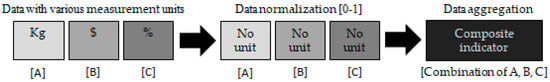
Figure 1.
Generalized graphical representation of normalization for constructing a composite indicator.
Every step of data transformation and/or normalization increases the probability of uncertainty and measurement error [30]. Accordingly, the choice of the proper normalization technique is indisputably important. In developing composite indicators, the selection of a preferred normalization technique deserves special care, taking into account the objectives of the composite indicators as well as the data properties and the potential requirement of further analysis [20,31]. Different normalization techniques produce different results [13] and may have major effects on composite scores [22,32].
2. Materials and Methods
For this paper, five normalization techniques are examined to investigate their effect and to identify the preferred technique for constructing composite indicators of coastal agricultural sustainability assessment in Bangladesh. Figure 2 shows the construction and evaluation process of the individual composite indicators that are examined in this paper. As shown in this figure, sustainability was categorized in terms of productivity, stability, efficiency, durability, compatibility, and efficiency. In brief, productivity is related to the yield of agricultural systems, stability refers to the ability to maintain a good level of productivity over an extended period of time, and efficiency is the measure of the extent to which the inputs for agricultural production enhance the crop yield. Durability can be defined as the ability of the agricultural system to resist or recover from stress and thereby maintain a good level of productivity over a cropping cycle. Compatibility refers to the ability of an agricultural system to fit in with the bio-geophysical, human, and socio-cultural surroundings in which the system is placed, and equity reflects a good quality of life for farmers and their family members [7]. For details about these categories, see vanLoon et al. [7]. For conceptual judging and selection of indicators, the dataset of Talukder [33] was used. Talukder [33] developed 110 indicators for assessing the sustainability of the coastal agricultural systems of Bangladesh. From 110 indicators of six sustainability categories, 50 indicators (Table A2, Table A3, Table A4, Table A5, Table A6 and Table A7 in Appendix B) were judged according to their importance and then grouped to make 15 composite indicators, as depicted in Figure 2. Then, various normalization, weighting, and aggregation techniques were applied to identify suitable normalization and aggregation techniques for developing the final set of composite indicators.
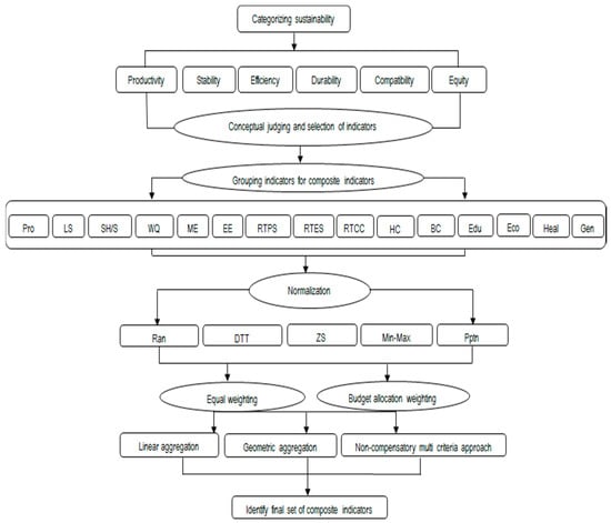
Figure 2.
Scheme for the construction and evaluation process for single composite indicators. Legend: Pro = Productivity; LS = Landscape stability; SH/S = Soil health/stability; WQ = Water quality; ME = Monetary efficiency; EE = Energy efficiency; RTPS = Resistance to pest stress; RTES = Resistance to economic stress; RTCC = Resistance to climate change; HC = Human compatibility; BC = Biophysical compatibility; Edu = Education; Eco = Economic; Heal = Health; Gen = Gender; Pptn = Proportionate; Ran = Ranking; DTT = Distance to target; CS = Categorical scale; Min-Max = Min-max technique; ZS = Z-score. Source: Compiled by the authors.
2.1. Overview of Datasets
The datasets in Table A2, Table A3, Table A4, Table A5, Table A6 and Table A7 in Appendix B contain different measurement units under six categories of sustainability. The data were collected from both primary and secondary sources in the southwest coastal zone of Bangladesh. The primary data were collected from five different agricultural systems: Bagda (shrimp)-based agricultural systems (S) from Shyamnagar; Bagda-rice-based agricultural systems (SR) from Kalijang; rice-based agricultural systems (R) from Kalaroa; Galda-rice-vegetable-based integrated agricultural systems (I) from Dumuria; and traditional practices-based agricultural systems (T) from Bhola Sadar (Figure 3). The details of the data collection process, justification of data collection, and development of indicators can be found in Talukder [33]. The description of the indicators, their units, data type, their relationships with sustainability pillars, data collection areas, data sources, and levels of measurement are presented in brief in Table A2, Table A3, Table A4, Table A5, Table A6 and Table A7 in Appendix B. A point to be noted here is that to develop the indicators, the collected data were processed through cleaning, integration, reduction, and transformation. No outliers were detected in the collected data during these processes.
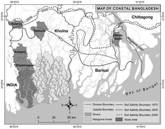
Figure 3.
Location of the study areas and gradients of soil salinity (1973–2009) in the coastal zone of Bangladesh. The soil salinity contours represent the northern boundary of areas where soils may have salinity values of 2 dS m−1 or more ([16], p. 149).
2.2. Normalization
A variety of transformation and/or normalization techniques are available (e.g., [29,34,35,36]), but only the five most widely employed techniques [35,37] are shown in Table 1. These five techniques are ranking, distance to target, Z-score, min-max, and proportionate normalization. The first four are the most commonly used normalization techniques [13,21]. The proportionate normalization technique was considered because of its suitability for the development of composite indicators.

Table 1.
Selected normalization techniques for this study.
2.2.1. Ranking Normalization
Ranking normalization replaces measurements with their rank. In the rank normalization process, each data point is replaced by its rank, that is, by values ranging from 1 (lowest) to N (highest) [38]. In this system, there is no score, only a rank; the absolute-level information is lost. This technique, while simple, cannot lead to any conclusion about the differences among performances of the indicator being assessed because there is no measure of the distance between values of the indicators [39]. Ranking normalization is employed in the “Information and Communications Technology Index” [29] and “Medicare Study on Healthcare Performance across the United States” [40].
2.2.2. Distance to Target Normalization
In the distance to target normalization technique, the indicator’s value is divided by the target value to normalize the indicator [21] so that the normalized values represent a fraction of the highest value. The highest value of the indicator set or any reference point can be the target value. The results of this technique are easy to handle and understand, but imbalance between scores and rankings remains, and the normalization results are more influenced by outliers than in other techniques. This method is useful for further analysis (e.g., geometric aggregation) since it does not generate any zero values. However, if outliers are chosen as target points, the result can be misleading. The distance to target normalization technique is used in “Eco-indicator 99” and the “Summary Innovation Index” [41].
2.2.3. Z-Score Normalization
Z-score normalization is calculated by subtracting the mean from an indicator value and then dividing by its standard deviation. If the standard deviation is calculated for a set of variables with a mean of 0 and then all values are divided by the standard deviation, the resulting set of values will have a standard deviation of 1 [27]. After performing normalization, the data have a common scale with a 0 mean and a standard deviation of 1. Since all Z-score distributions have the same mean and standard deviation, individual scores from different distributions can be directly compared. The advantage of this technique is that it provides no distortion from the mean, adjusting for different scales and variance. The output is dimensionless, and the relative differences are maintained due to the application of a linear transformation [42]. Z-score is preferred when extreme values exist in the dataset [20,32]. Although the technique does not fully adjust for outliers, the minimum and maximum values are not as influential as in other techniques such as distance to target. When extreme values are present in the original data, Z-score normalization takes these extreme values into account in a manner that does not distort their impacts on a composite indicator. In this way, an outlier, such as exceptional performance, is recognized and not ignored [13,27]. The Z-score technique is widely employed, including in the knowledge-based economy index [43] and the World Health Organization’s child growth standards index [44].
2.2.4. Min-Max Normalization
The min-max technique rescales data into different intervals based on minimum and maximum values. The advantage of this method is that boundaries can be set and all indicators have an identical range (0, 1). However, the normalized values do not maintain proportionality, and normalized values reflect the percentage of the range of . This technique is based on extreme values (minimum and maximum), but because these two values can be outliers, the range of max and min strongly influences the final output. Another disadvantage is that the difference in variance is not fully eliminated [13]. Nevertheless, this technique is very popular and has been applied in the construction of many composite indicators, the best-known of which is the Human Development Index (HDI, [45]).
2.2.5. Proportionate Normalization
In proportionate normalization, the single attribute value is divided by the sum total of the values of attributes [37,46]. The normalized values maintain proportionality such that they reflect the percentage of the sum of the total value of the indicators. Here, values of the indicator are relatively normalized. Normalizing the indicators by dividing them by their sums has a number of attractive properties, including that the normalized values are identical to the original, except for a scaling factor, and the process is easily understandable. The value differences among indicators become narrow. Dividing by the sum ensures that even the smallest value greater than zero comes out with a positive normalized value [19,37]. The proportionate normalization technique is frequently used in normalizing census data in ArcView GIS (Geographical Information System, [46]). Benini [19] also suggested using this technique for developing composite measures for disaster impact assessment.
2.3. Weighting
The final score and ranking of the composite indicators depends on the weighting of the normalized values of the indicators. Weighting reflects the importance of each indicator relative to the overall composite indicators [21]. Weights should ideally be selected according to an underlying and agreed-upon, or at least clearly stated theoretical, framework so that the process is transparent [47,48]. Weighting can be a very important step in creating composite indicators before aggregation can take place, because it modifies the sub-indicator values. However, Sajeva et al. [28] have shown that the use of different weighting schemes can often have no significant effect on the ranking of the composite indicators. No agreed-upon methodology exists to weight individual indicators. Different types of weighting techniques and their explanations are provided by Nardo et al. [20].
In this paper, equal weighting of sub-indicators is used for all rank, distance to target, Z-score, max-min and proportionate normalization, and arithmetic mean and geometric mean aggregation. Simplicity is the main advantage of equal weighting, but the composite indicator that is developed by the combination of more indicators will have a stronger influence on the list of composite indicators. Using this weighting system may be justified when no other available means of weighting are known [30]. Equal weighting is used in the HDI [49]. Budget allocation techniques for weighting are used for MCA aggregation (as shown in Table A13). A budget allocation technique for weighting is chosen because the sustainability of agriculture is very contextual, so stakeholders’ opinions are very important for weighting of the indicators. Geometric and multi-criteria, as well as linear, aggregation can be employed with these weightings [13]. The OECD’s Handbook on Constructing Composite Indices [13] describes expert weighting as a budget allocation technique. In expert weighting, an expert allocates 100 points among indicators according to their importance [21]. Selection of the appropriate expert and number of experts is the biggest problem for this system because point allocation may be influenced by the expert’s experience [30]. This subjective judgment of the weights of sub-indicators is used to allocate relative worth for each sub-indicator [22]. Subjective weighting is often affected by strong inter-individual disagreement [29] and is particularly sensitive in the case of complex, interrelated, and multidimensional phenomena [20]. Nevertheless, Sen and Foster ([48], p. 206) pointed out that “while the possibility of arriving at a unique set of weights is rather unlikely, that uniqueness is not really necessary to make acceptable judgments in many situations, and may indeed not even be required for a complete ordering”.
2.4. Aggregation
The rules for aggregation are well documented in the Handbook on Constructing Composite Indices [13], but steps are still debated in the development of composite indicators [50]. The fundamental issue in aggregation is the compensability of indicators, which is defined as compensating for any indicator’s dimension with a suitable surplus in another indicator’s dimension. The rules for aggregating composite indicators can be compensatory or non-compensatory [51]. A compensatory technique deals with the imbalances in the indicators and uses linear functions, whereas non-compensatory techniques use unbalance-adjusted functions [52]. Different aggregation rules are possible to develop composite indicators. Commonly applied aggregation options include additive aggregation (arithmetic mean), geometric aggregation (multiplication), and multi-criteria analysis [13].
The arithmetic mean is a linear function [53]. The normalized and weighted or unweighted indicators are summed to compute the arithmetic mean (the formula for evaluating arithmetic mean is ) [26,32]. In this method, compensability can be a disadvantage if a low value in one indicator or dimension masks a high value in another, that is, a deficit in one indicator or dimension can be compensated for by a surplus in another [30,32].
Geometric aggregation, which is the product of normalized weighted indicators, is used to avoid concerns related to interaction and compensability [32]. Non-comparable data measured in a ratio scale can only be meaningfully aggregated by using geometric functions, provided that indicators are strictly positive [20,30]. A geometric mean (the formula for evaluating geometric mean is ) takes into consideration differences in achievement across dimensions [20]. Poor performance in any dimension or indicator is directly reflected in the composite indicator’s value. According to Hudrlikova and Kramulova [30], this technique is partly compensable since it rewards composite indicators with higher indicator scores.
“When different goals are equally legitimate and important, and in addition trade-offs exist between the dimensions of a composite indicator (namely negative correlations between dimensions) then a non-compensatory logic may be necessary” ([21], p. 256). Multi-Criteria Analysis (MCA) is used for aggregating non-compensatory data [52]. In general, MCA provides an overall ranking based on the weight and values of given indicators. One of the shortcomings of MCA is that when the number of indicators to develop composite indicators is high, it is difficult to compute MCA [30]. MCA is based on an outranking matrix. The standard procedure for performing an MCA consists of three steps: identifying the weighting of the criteria, preparing an “outranking matrix” by pairwise comparison of the weighted performance of each criterion (for n options, there are n (n − 1)/2 comparisons) [54], and calculating the composite indicator score of the criteria by adding the values of the row of the outranking matrix [55].
2.5. Robustness
The outcome of the composite indicators depends on the selection of variables, normalization, weighting (if it is used), and aggregation techniques [20], so it is necessary to examine the robustness of the developed composite indicators. Various statistical tests can help ensure that the composite is reliable. Freudenberg [29] and Hudrlikova and Kramulova [30] mentioned correlation as a technique to assess the impacts of different normalization techniques on composite indicators. The correlation coefficient can show whether the results of the composite indicator are heavily influenced by the choice of normalization rules [30] and aggregation methods. In this paper, correlation is used to assess the robustness of composite indicators.
3. Results
The results for the composite indicators using various normalization techniques, weighting, and different aggregation techniques are presented in Table A8, Table A9, Table A10, Table A11, Table A12 and Table A13 in Appendix B. The results of the robustness tests of the composite indicators are presented in Table A14, Table A15, Table A16, Table A17, Table A18, Table A19, Table A20, Table A21, Table A22, Table A23, Table A24, Table A25, Table A26 and Table A27 in Appendix B.
The values of data and different normalization techniques and arithmetic aggregation involve different assumptions that have specific consequences that produce different results for the composite indicators (Table A8, Table A9, Table A10, Table A11, Table A12 and Table A13). In this regard, Nardo et al. [20] mentioned that the ranking of composite indicators is heavily influenced by the nature of the data. Saisana and Saltelli [21] also pointed out that it is beyond doubt that composite indicators are a value-laden construct. In arithmetic aggregation, it is also observed that poor performance in some indicators is covered by sufficiently high values of other indicators in composite indicators.
In the dataset for this study, the score for some of the indicators is “0”. For example, as shown in Table A6, in the compatibility category “S” scored “0” in drinking water quality. Indicators that have “0” scores have the normalization result “0” in proportionate, distance, and Z-score normalization, but not a “0” ranking normalization, since the score “0” is ranked as the lowest number. The max-min normalization also generates “0” scores as normalized values. Whenever the normalization score is “0” or negative, those indicators are not suitable for geometric mean aggregation because geometric aggregation requires all positive numbers and is therefore only appropriate when indicator values are always positive [20].
When aggregation was carried out considering indicators’ values and budget allocation weight and MCA techniques, the results also generated different values for some of the composite indicators (Table A13) compared to other types of aggregation. Due to the nature of the data, MCA also generates “0” values for productivity, energy efficiency, and human compatibility composite indicators of “S”, as well as “0” values for resistance to economic stress, resistance to climate change, and gender composite indicators of “T” (Table A13). Therefore, budget allocation weighting and MCA combinations cannot be recommended for composite indicators.
These different values of the composite indicators that result from applying different combinations of normalization techniques, weighting, and aggregation reflect that the properties of the indicators are very crucial for the final output values of the composite indicators. This study shows that the normalization technique, arithmetic mean, and geometric mean should take into account the data properties, as well as the objectives of the composite indicator. From the results, it appears that not all normalization techniques are suitable for the dataset, and not all normalization techniques support arithmetic mean and geometric mean. Even when MCA techniques are applied, some “0” values are generated for the composite indicators.
Nardo et al. [20] suggested that in the case of non-compensatory composite indicators, MCA is the best way to develop indicator values. However, due to the nature of the present dataset, MCA is not suitable for this experiment because the “0” scores of some of the indicators do not reflect the weight of the indicator, so the results may be difficult to interpret and compare. In MCA, composite indicators are based on weight, so the magnitudes of values of the different indicators are disregarded in the composite. “This means any issue that does marginally better on many indicators score higher than the issue that does a lot better on a few indicators because outstanding performances of the indicators cannot compensate for the deficiencies in some indicators” ([56], p. 364).
4. Discussion
In this study, it is observed that proportionate normalization produced values that conserve the proportionality of the indicator values (Table A12), whereas other normalization techniques show different outcomes. For example, the normalization results of rank, distance to target, Z-score, max-min, and proportionate normalization for weighted yield of rice indicators of “S” in Table A8, Table A9, Table A10, Table A11 and Table A12 are 1, 0.35, −1, 0 and 0.11, respectively. Here, only the 0.11 that is generated using proportionate normalization represents the proportionate value of the original score of 2.26 for the weighted yield of rice indicator of “S” (see Table A2). Therefore, proportionate normalization is selected to develop composite indicators in this study, because the original values of the data do not change through this process. If the values of the data change due to the transformation technique/normalization, they are mathematically not meaningful. Therefore, it is always preferable to follow a technique by which original data are transformed in such a way that their informational content is not fundamentally altered [22]. In proportionate normalization, the rank of the composite indicator depends on actual values since proportionate normalization does not alter the actual importance of the values of the indicators. This is the strength of this technique [22]. Furthermore, proportionate normalization seems preferable in this experiment to the most popular min-max normalization because there are no goalpost values for any of the 50 indicators.
There is clearly no universal best aggregation method because aggregation depends on the requirement of the developer of the composite indicators. In the data there are some “0” values. Therefore, to aggregate the indicators, a hybrid aggregation is suggested: indicator values with the “0” normalization result will be aggregated by arithmetic mean, and the rest will be aggregated by geometric mean. Hybrid aggregation techniques use more than one aggregation function at different levels [54]. For example, the “Multidimensional Poverty Assessment Tool (UNIFAD, 2010 as cited in [54]) used arithmetic average within a subcomponent and geometric average within a component, while the Food and Nutrition Security Index (FAO, 2014 as cited in [57]) used arithmetic averages within dimensions and geometric average across dimensions” ([57], p. 16). When comparing all applied normalization and aggregation techniques, it appeared that, for the present research, the proportionate normalization and hybrid aggregation techniques (geometric mean and arithmetic mean) produced the most preferred results. Therefore, 15 single composite indicators are developed from the 50 indicators in Talukder et al. [16] using proportionate normalization and hybrid aggregation. These 15 single composite indicators (see Table 2) are proposed to create a set of the most representative variables of agricultural sustainability in the study area. Among these 15 composite indicators, “monetary efficiency” carries the proportionate normalization values of the original values without any aggregation but is normalized by proportionate normalization.
Table 2.
Composite indicators developed using proportionate normalization and hybrid aggregation techniques.
5. Conclusions
This study tested various normalization and aggregation techniques for developing composite indicators, providing a comparison among different combinations to find out the best normalization and aggregation combination. Normalization techniques, weighting, and aggregation all influence the final outcomes of composite indicators, so it is important to compare different combinations of normalization, weighting, and aggregation techniques. Rank, distance to target, Z-score, max-min, and proportionate methods were used for normalization, while equal weight and budget allocation for weighting and arithmetic mean, geometric mean, and multi-criteria analysis were used for aggregation. The results show that the normalization and characteristics of data have a huge influence on composite indicators. For example, the human compatibility composite indicator in the compatibility category has a score of “0” using rank normalization and geometric aggregation, distance to target normalization and geometric mean, Z-score normalization and arithmetic mean, Z-score normalization and geometric mean, max-min normalization and arithmetic mean, proportionate normalization and geometric mean, proportionate normalization and arithmetic mean, or MCA. A score of 1 results from using rank normalization and arithmetic mean, a score of 0.25 from using distance to target normalization and arithmetic mean, and a score of −1.98 using Z-score normalization and arithmetic mean.
Both methodological and empirical conclusions can be drawn from this study. From a methodological point of view, it can be said that proportionate normalization and the hybrid aggregation technique are suitable for developing composite indicators from these empirical data, which are developed through a questionnaire and secondary data and have a score of “0” for several indicators. These techniques allow the aggregation of a multidimensional set of indicators into a unique composite indicator that can facilitate the understanding of a complex concept such as agricultural sustainability. In the case of proportionate normalization, weighting the indicators has no effect. However, these techniques depend on the properties of the indicators, and some subjectivity is associated with the selection of normalization and aggregation rules. Depending on the methodology selected for constructing indicators, the results of the composite indicators can vary and sometimes be misleading. Based on the properties of the dataset, it appears that proportionate normalization is appropriate, and a hybrid of aggregation rules is suitable for developing composite indicators. However, it is the responsibility of the designer of the composite indicator to choose the most appropriate normalization and aggregation techniques. These techniques must have a sound and transparent methodological framework. In this respect Nardo et al. [20] also stated that the selection of the normalization process deserves special care.
Acknowledgments
This paper has been supported by the Social Sciences and Humanities Research Council (SSHRC), Canada.
Author Contributions
Byomkesh Talukder conceived and designed the original research as part of his Ph.D. thesis. Keith W. Hipel helped to execute the research and Gary W. vanLoon guided the statistical techniques to develop criteria.
Conflicts of Interest
The authors declare no conflict of interest.
Appendix A
Table A1.
Checklist for building a composite indicator.
Table A1.
Checklist for building a composite indicator.
| Steps | Description | Why It Is Needed |
|---|---|---|
| 1st: Theoretical framework | Provides the basis for the selection and combination of variables into a meaningful composite indicator under a fitness-for-purpose principle (involvement of experts and stakeholders is envisioned in this step). |
|
| 2nd: Data selection | Should be based on the analytical soundness, measurability, country coverage, and relevance of the indicators to the phenomenon being measured and their relationship to each other. The use of proxy variables should be considered when data are scarce (involvement of experts and stakeholders is envisioned in this step). |
|
| 3rd: Imputation of missing data | Is needed in order to provide a complete dataset (e.g., by means of single or multiple imputation). |
|
| 4th: Multivariate analysis | Should be used to study the overall structure of the dataset, assess its suitability, and guide subsequent methodological choices (e.g., weighting, aggregation). |
|
| 5th: Normalization | Should be carried out to render the variables comparable. |
|
| 6th: Weighting and aggregation | Should be done along the lines of the underlying theoretical framework. |
|
| 7th: Uncertainty and sensitivity analysis | Should be undertaken to assess the robustness of the composite indicator in terms of the mechanism for including or excluding an indicator, the normalization scheme, the imputation of missing data, the choice of weights, the aggregation method, and so forth. |
|
| 8th: Back to the data | Is needed to reveal the main drivers of overall good or bad performance. Transparency is primordial to good analysis and policymaking. |
|
Source: [13], pp. 20–22.
Appendix B
Table A2.
Selected indicators and values to construct single composite indicators for productivity.
Table A2.
Selected indicators and values to construct single composite indicators for productivity.
| Sustainability Category | Composite Indicator | Description | Unit | Data Type | Sustainability Pillar | Data Source | Weighting | Study Areas | Level of Measurement | ||||
|---|---|---|---|---|---|---|---|---|---|---|---|---|---|
| S | SR | R | I | T | |||||||||
| Productivity | Productivity | Weighted yield of the main staple crop | t/ha | QTL | Economic | QS | 0.4 | 2.26 | 4.41 | 5.23 | 6.51 | 2.86 | Ratio scale |
| Net income from the agro-ecosystem | $/ha | QTL | Economic | QS | 0.4 | 311.15 | 1020.37 | 1585.81 | 1806.04 | 544.01 | Ratio scale | ||
| Protein yield from the agro-ecosystem | kg/ha | QTL | Ecological | QS | 0.2 | 68.42 | 147.23 | 552 | 373.01 | 318.87 | Ratio scale | ||
Legend: QNT = Quantitative; QS = Questionnaire survey.
Table A3.
Selected indicators and values to construct single composite indicators for stability.
Table A3.
Selected indicators and values to construct single composite indicators for stability.
| Sustainability Category | Composite Indicator | Description | Unit | Data Type | Sustainability Pillar | Data Source | Weighting | Study Areas | Level of Measurement | ||||
|---|---|---|---|---|---|---|---|---|---|---|---|---|---|
| S | SR | R | I | T | |||||||||
| Stability | Landscape stability | Land exposure to natural events: cyclone | binary yes/no response | QUAL | Ecological | SD | 0.3 | 1 | 2 | 2 | 2 | 1 | Nominal scale |
| Land exposure to natural events: saline water | binary yes/no response | QUAL | Ecological | SD | 0.3 | 1 | 1 | 3 | 2 | 3 | Nominal scale | ||
| Land exposure to natural events: drought in kharif to rabi season | binary yes/no response | QUAL | Ecological | SD | 0.05 | 1.5 | 1.5 | 2 | 2 | 3.5 | Nominal scale | ||
| Land exposure to natural events: river bank erosion | binary yes/no response | QUAL | Ecological | SD | 0.05 | 2 | 2 | 2 | 2 | 1 | Nominal scale | ||
| Stability of embankment | binary yes/no response | QUAL | Ecological | FO | 0.2 | 1 | 2 | 1 | 2 | 2 | Nominal scale | ||
| Withdrawal of upstream water | binary yes/no response | QUAL | Ecological | SD | 0.1 | 1 | 1 | 1 | 1 | 2 | Nominal scale | ||
| Soil health/stability | Organic materials | % | QTL | Ecological | SD | 0.3 | 4 | 4 | 2 | 3 | 2 | Ordinal scale | |
| Salinity | dS/m | QTL | Ecological | SD | 0.35 | 1 | 5 | 6 | 3 | 6 | Ordinal scale | ||
| Macronutrient: N | meq/100 g | QTL | Ecological | SD | 0.1 | 2 | 2 | 2 | 1 | 2 | Ordinal scale | ||
| Macronutrient: P | meq/100 g | QTL | Ecological | SD | 0.1 | 3 | 2 | 3 | 3 | 3 | Ordinal scale | ||
| Macronutrient: K | meq/100 g | QTL | Ecological | SD | 0.1 | 6 | 4 | 3 | 2 | 4 | Ordinal scale | ||
| Soil pH | Ratio (no unit) | QTL | Ecological | SD | 0.05 | 1 | 3 | 4 | 2 | 4 | Ordinal scale | ||
| Water quality | Water salinity in surface water (quality of surface water for irrigation) | dS/m | QTL | Ecological | SD | 0.4 | 1 | 2 | 2 | 2 | 3 | Ordinal scale | |
| Water salinity in groundwater (quality of groundwater for irrigation) | dS/m | QTL | Ecological | SD | 0.4 | 1 | 2 | 2 | 4 | 3 | Ordinal scale | ||
| Arsenic concentration (quality of groundwater for irrigation) | ppm | QTL | Ecological | SD | 0.2 | 2 | 2 | 2 | 2 | 4 | Ordinal scale | ||
Legend: QNT = Quantitative; QUAL = Qualitative; SD = Secondary data; FO = Field observation.
Table A4.
Selected indicators and values to construct single composite indicators for efficiency.
Table A4.
Selected indicators and values to construct single composite indicators for efficiency.
| Sustainability Category | Composite Indicator | Description | Unit | Data Type | Sustainability Pillar | Data Source | Weighting | Study Areas | Level of Measurement | ||||
|---|---|---|---|---|---|---|---|---|---|---|---|---|---|
| S | SR | R | I | T | |||||||||
| Efficiency | Monetary efficiency | Money input and output in the agro-ecosystem | $ output/$ input | QTL | Economic | QS | 1 | 1.53 | 2.24 | 2.78 | 6.67 | 2.29 | Ratio scale |
| Energy efficiency | Overall energy efficiency | Ratio of energy output and input | QTL | Ecological | QS | 0.6 | 1.37 | 2.01 | 5.53 | 5.54 | 5.9 | Ratio scale | |
| Non-renewable energy efficiency | Ratio of energy output and input | QTL | Ecological | QS | 0.4 | 0.78 | 0.92 | 2.17 | 2.52 | 2.44 | Ratio scale | ||
Legend: QNT = Quantitative; QS = Questionnaire survey.
Table A5.
Selected indicators and values to construct single composite indicators for durability.
Table A5.
Selected indicators and values to construct single composite indicators for durability.
| Sustainability Category | Composite Indicators | Description | Unit | Data Type | Sustainability Pillar | Data Source | Weighting | Study Areas | Level of Measurement | ||||
|---|---|---|---|---|---|---|---|---|---|---|---|---|---|
| S | SR | R | I | T | |||||||||
| Durability | Resistance to pest stress | Chemical response to pest stress | binary yes/no response | QUAL | Ecological | QS | 0.25 | 1.78 | 4.17 | 4.24 | 5.45 | 6.54 | Nominal scale |
| Water availability at transplanting stage of rice | binary yes/no response | QUAL | Ecological | QS | 0.25 | 0.75 | 0.75 | 0.2 | 0.2 | 0.2 | Nominal scale | ||
| Water availability at flowering stage of rice | binary yes/no response | QUAL | Ecological | QS | 0.25 | 0.75 | 0.75 | 0.2 | 0.2 | 0.2 | Nominal scale | ||
| Farm management (soil test, pest management, land management, soil fertility management) | binary yes/no response | QUAL | Ecological | QS | 0.25 | 0.67 | 0.83 | 1.69 | 1.36 | 0.0 | Nominal scale | ||
| Resistance to economic stress | Good product price | binary yes/no response | QUAL | economic | QS | 0.35 | 8.44 | 5 | 4.58 | 4.55 | 3.8 | Nominal scale | |
| Availability of seeds | binary yes/no response | QUAL | Ecological | QS | 0.3 | 9.33 | 9.5 | 10 | 10 | 8.85 | Nominal scale | ||
| Availability of market (market diversification) | binary yes/no response | QUAL | Social/economic | QS | 0.35 | 10 | 9.17 | 8.47 | 10 | 7.69 | Nominal scale | ||
| Resistance to climate change | Agricultural training | binary yes/no response | QUAL | Social/ecological | QS | 0.4 | 1.33 | 1.83 | 0.33 | 2.27 | 1.15 | Nominal scale | |
| Climate change awareness | binary yes/no response | QUAL | Social | QS | 0.3 | 1.11 | 0.67 | 0.51 | 1.82 | 0 | Nominal scale | ||
| Advice from agricultural extension workers or NGO | binary yes/no response | QUAL | Ecological | QS | 0.3 | 0.66 | 1.17 | 0.51 | 0.45 | 0.38 | Nominal scale | ||
Legend: QUAL = Qualitative; QS = Questionnaire survey.
Table A6.
Selected indicators to construct single composite indicators for compatibility.
Table A6.
Selected indicators to construct single composite indicators for compatibility.
| Sustainability Category | Composite Indicators | Description | Unit | Data Type | Sustainability Pillar | Data Source | Weighting | Study Areas | Level of Measurement | ||||
|---|---|---|---|---|---|---|---|---|---|---|---|---|---|
| S | SR | R | I | T | |||||||||
| Compatibility | Human Compatibility | Drinking water quality (protected) | binary yes/no response | QUAL | Ecological | QS | 0.5 | 0 | 8 | 9 | 10 | 9 | Nominal scale |
| Illness from drinking water | binary yes/no response | QUAL | Ecological | QS | 0.5 | 5 | 10 | 10 | 10 | 10 | Nominal scale | ||
| Biophysical Compatibility | Overall biodiversity condition: percentage of non-crop area | % | QTL | Ecological | QS | 0.25 | 7.54 | 6.48 | 23.01 | 15.73 | 18.68 | Ordinal scale | |
| Overall biodiversity condition: crop richness | number of crops | QTL | Ecological | QS | 0.25 | 2 | 6 | 16 | 10 | 17 | Ordinal scale | ||
| Overall biodiversity condition: crop rotation | number | QTL | Ecological | QS | 0.25 | 2 | 3 | 5 | 4 | 4 | Ordinal scale | ||
| Ecosystem connectivity | binary yes/no response | QUAL | Ecological | FO | 0.25 | 1 | 1 | 2 | 2 | 2 | Nominal scale | ||
Legend: QNT = Quantitative; QUAL = Qualitative; QS = Questionnaire survey; FO = Field observation.
Table A7.
Selected indicators and values to construct single composite indicators for equity.
Table A7.
Selected indicators and values to construct single composite indicators for equity.
| Sustainability Category | Composite Indicators | Description | Unit | Data Type | Sustainability Pillar | Data Source | Weighting | Study Areas | Level of Measurement | ||||
|---|---|---|---|---|---|---|---|---|---|---|---|---|---|
| S | SR | R | I | T | |||||||||
| Equity | Education | Education of farmers | % | QTL | Social | QS | 0.25 | 8.56 | 9.25 | 4.75 | 10 | 5 | Ordinal scale |
| Education status of farmers’ male children | % | QTL | Social | QS | 0.25 | 10 | 9.49 | 11.2 | 13.1 | 7.45 | Ordinal scale | ||
| Education status of farmers’ female children | % | QTL | Social | QS | 0.25 | 9.07 | 10.54 | 11.17 | 12.5 | 6.36 | Ordinal scale | ||
| Access to electronic media | % | QTL | Social | QS | 0.25 | 7.78 | 9.17 | 9.39 | 10 | 3.08 | Ordinal scale | ||
| Economic | Farm profitability | $ | QTL | Economic | QS | 0.2 | 648.23 | 3340.55 | 1371.32 | 1992.39 | 1025.06 | Ratio scale | |
| Average wage of farm labourer ($) | $/person/day | QTL | Economic | QS | 0.2 | 1.33 | 1.33 | 1.60 | 1.80 | 1.60 | Ratio scale | ||
| Livelihood diversity other than agriculture | Count, 0 to 5 | QTL | Economic | QS | 0.2 | 6.22 | 4.33 | 5.93 | 4.55 | 6.92 | Ordinal scale | ||
| Years of economic hardship | Number of years | QTL | Economic | QS | 0.2 | 0.73 | 0.73 | 0.91 | 0.82 | 0.64 | Ordinal scale | ||
| Road network (establishing farm roads and access roads) | access/no access | QTL | Economic/social | QS | 0.2 | 2 | 3 | 3 | 3 | 1 | Nominal scale | ||
| Health | Settings where treatment is taken or public health | % | QTL | Social | QS | 0.5 | 3.51 | 4.76 | 4.07 | 8.14 | 4.29 | Ordinal scale | |
| Sanitation or public health | % | QTL | Social | QS | 0.5 | 7.69 | 8.73 | 7.59 | 7.41 | 7.08 | Ordinal scale | ||
| Gender | Women’s involvement in decision making about agricultural activities | % | QTL | Social | QS | 0.5 | 3 | 4 | 5 | 6.5 | 2.5 | Ordinal scale | |
| Gender-based wage differentials | $/person/day | QTL | Economic | QS | 0.5 | 0.33 | 0.33 | 0.5 | 0.59 | 0 | Ratio scale | ||
Legend: QNT = Quantitative; QS = Questionnaire survey.
Table A8.
Results of composite indicators after applying rank normalization and aggregation techniques.
Table A8.
Results of composite indicators after applying rank normalization and aggregation techniques.
| Results of Rank Normalization and Geometric Mean | ||||||
| Category | Composite indicators | S | SR | R | I | T |
| Productivity | Productivity | 1.00 | 2.62 | 4.31 | 4.64 | 2.29 |
| Stability | Landscape stability | 1.12 | 1.41 | 1.70 | 1.78 | 1.82 |
| Soil health/stability | 1.91 | 2.33 | 2.24 | 1.59 | 2.40 | |
| Water quality | 1.00 | 1.59 | 1.59 | 2.00 | 2.62 | |
| Efficiency | Monetary efficiency * | 0.10 | 0.14 | 0.18 | 0.43 | 0.15 |
| Energy efficiency | 1.00 | 2.00 | 3.00 | 4.47 | 4.47 | |
| Durability | Resistance to pest stress | 1.68 | 2.21 | 1.97 | 2.00 | 1.71 |
| Resistance to economic stress | 3.42 | 3.30 | 2.88 | 3.17 | 1.00 | |
| Resistance to climate change | 3.17 | 3.91 | 1.82 | 3.68 | 0.14 | |
| Compatibility | Human compatibility | 1.00 | 2.00 | 2.45 | 2.83 | 2.45 |
| Biophysical compatibility | 1.19 | 1.41 | 3.56 | 2.71 | 3.31 | |
| Equity | Education | 2.45 | 2.91 | 3.36 | 5.00 | 1.19 |
| Economic | 1.74 | 2.27 | 2.93 | 2.93 | 1.82 | |
| Health | 2.00 | 4.47 | 2.45 | 3.16 | 1.73 | |
| Gender | 1.41 | 2.45 | 3.46 | 4.47 | 1.00 | |
| Results of Rank Normalization and Arithmetic Mean | ||||||
| Category | Composite indicators | S | SR | R | I | T |
| Productivity | Productivity | 1.00 | 2.67 | 4.33 | 4.67 | 2.33 |
| Stability | Landscape stability | 1.17 | 1.50 | 1.83 | 1.83 | 2.00 |
| Soil health/stability | 2.17 | 2.50 | 2.50 | 1.67 | 2.67 | |
| Water quality | 1.00 | 1.67 | 1.67 | 2.33 | 2.67 | |
| Efficiency | Monetary efficiency * | 0.10 | 0.14 | 0.18 | 0.43 | 0.15 |
| Energy efficiency | 1.00 | 2.00 | 3.00 | 4.50 | 4.50 | |
| Durability | Resistance to pest stress | 1.75 | 2.25 | 2.50 | 2.50 | 2.00 |
| Resistance to economic stress | 3.67 | 3.33 | 3.00 | 3.33 | 1.00 | |
| Resistance to climate change | 3.33 | 4.00 | 2.00 | 4.00 | 1.67 | |
| Compatibility | Human compatibility | 1.00 | 2.00 | 2.50 | 3.00 | 2.50 |
| Biophysical compatibility | 1.25 | 1.50 | 3.75 | 2.75 | 3.50 | |
| Equity | Education | 2.50 | 3.00 | 3.50 | 5.00 | 1.25 |
| Economic | 2.00 | 2.60 | 3.00 | 3.00 | 2.20 | |
| Health | 2.50 | 4.50 | 2.50 | 3.50 | 2.00 | |
| Gender | 1.50 | 2.50 | 3.50 | 4.50 | 1.00 | |
Legend: S = Bagda (shrimp)-based agricultural systems (S) from Shyamnagar, SR = Bagda-rice-based agricultural systems (SR) from Kalijang, R = Rice-based agricultural systems (R) from Kalaroa, I = Galda-rice-vegetable-based integrated agricultural systems (I) from Dumuria and T = traditional practices-based agricultural systems (T) from Bhola Sadar. * Only proportionate normalization, no aggregation.
Table A9.
Results of composite indicators after applying distance to target normalization and aggregation techniques.
Table A9.
Results of composite indicators after applying distance to target normalization and aggregation techniques.
| Results of Distance to Target Normalization and Geometric Mean | ||||||
| Category | Composite indicators | S | SR | R | I | T |
| Productivity | Productivity | 0.19 | 0.47 | 0.89 | 0.88 | 0.42 |
| Stability | Landscape stability | 0.51 | 0.64 | 0.72 | 0.76 | 0.79 |
| Soil health/stability | 0.59 | 0.81 | 0.79 | 0.56 | 0.83 | |
| Water quality | 0.35 | 0.55 | 0.55 | 0.69 | 0.91 | |
| Efficiency | Monetary efficiency * | 0.10 | 0.14 | 0.18 | 0.43 | 0.15 |
| Energy efficiency | 0.27 | 0.35 | 0.90 | 0.97 | 0.98 | |
| Durability | Resistance to pest stress | 0.57 | 0.75 | 0.46 | 0.47 | 0.41 |
| Resistance to economic stress | 0.98 | 0.80 | 0.77 | 0.81 | 0.67 | |
| Resistance to climate change | 0.59 | 0.67 | 0.26 | 0.73 | 0.14 | |
| Compatibility | Human compatibility | #NUM! | 0.89 | 0.95 | 1.00 | 0.95 |
| Biophysical compatibility | 0.30 | 0.42 | 0.98 | 0.75 | 0.90 | |
| Equity | Education | 0.78 | 0.85 | 0.76 | 1.00 | 0.46 |
| Economic | 0.59 | 0.82 | 0.79 | 0.81 | 0.58 | |
| Health | 0.62 | 0.76 | 0.66 | 0.92 | 0.65 | |
| Gender | 0.24 | 0.27 | 0.38 | 0.47 | #NUM! | |
| Results of Distance to Target Normalization and Arithmetic Mean | ||||||
| Category | Composite indicators | S | SR | R | I | T |
| Productivity | Productivity | 0.21 | 0.50 | 0.89 | 0.89 | 0.44 |
| Stability | Landscape stability | 0.54 | 0.71 | 0.76 | 0.79 | 0.83 |
| Soil health/stability | 0.74 | 0.82 | 0.83 | 0.60 | 0.86 | |
| Water quality | 0.36 | 0.56 | 0.56 | 0.72 | 0.92 | |
| Efficiency | Monetary efficiency * | 0.10 | 0.14 | 0.18 | 0.43 | 0.15 |
| Energy efficiency | 0.27 | 0.35 | 0.90 | 0.97 | 0.98 | |
| Durability | Resistance to pest stress | 0.67 | 0.78 | 0.55 | 0.54 | 0.38 |
| Resistance to economic stress | 0.98 | 0.82 | 0.80 | 0.85 | 0.70 | |
| Resistance to climate change | 0.59 | 0.72 | 0.29 | 0.79 | 0.28 | |
| Compatibility | Human compatibility | 0.25 | 0.90 | 0.95 | 1.00 | 0.95 |
| Biophysical compatibility | 0.34 | 0.43 | 0.99 | 0.77 | 0.90 | |
| Equity | Education | 0.78 | 0.85 | 0.79 | 1.00 | 0.47 |
| Economic | 0.66 | 0.83 | 0.83 | 0.83 | 0.65 | |
| Health | 0.66 | 0.79 | 0.68 | 0.92 | 0.67 | |
| Gender | 0.33 | 0.35 | 0.51 | 0.61 | 0.04 | |
Legend: S = Bagda (shrimp)-based agricultural systems (S) from Shyamnagar, SR = Bagda-rice-based agricultural systems (SR) from Kalijang, R = Rice-based agricultural systems (R) from Kalaroa, I = Galda-rice-vegetable-based integrated agricultural systems (I) from Dumuria and T = traditional practices-based agricultural systems (T) from Bhola Sadar. * Only proportionate normalization, no aggregation. #NUM! means calculation is not possible.
Table A10.
Results of composite indicators after applying Z-score normalization and aggregation techniques.
Table A10.
Results of composite indicators after applying Z-score normalization and aggregation techniques.
| Results of Z-Score Normalization and Geometric Mean | ||||||
| Category | Composite indicators | S | SR | R | I | T |
| Productivity | Productivity | #NUM! | #NUM! | 0.96 | 0.97 | #NUM! |
| Stability | Landscape stability | #NUM! | #NUM! | #NUM! | #NUM! | #NUM! |
| Soil health/stability | #NUM! | #NUM! | #NUM! | #NUM! | #NUM! | |
| Water quality | #NUM! | #NUM! | #NUM! | #NUM! | 1.23 | |
| Efficiency | Monetary efficiency * | 0.10 | 0.14 | 0.18 | 0.43 | 0.15 |
| Energy efficiency | #NUM! | #NUM! | 0.63 | 0.86 | 0.91 | |
| Durability | Resistance to pest stress | #NUM! | #NUM! | #NUM! | #NUM! | #NUM! |
| Resistance to economic stress | #NUM! | #NUM! | #NUM! | #NUM! | #NUM! | |
| Resistance to climate change | #NUM! | #NUM! | #NUM! | #NUM! | 0.14 | |
| Compatibility | Human compatibility | #NUM! | 0.33 | 0.50 | 0.62 | 0.50 |
| Biophysical compatibility | #NUM! | #NUM! | 1.12 | #NUM! | 0.71 | |
| Equity | Education | #NUM! | #NUM! | #NUM! | 1.16 | #NUM! |
| Economic | #NUM! | #NUM! | #NUM! | #NUM! | #NUM! | |
| Health | #NUM! | #NUM! | #NUM! | #NUM! | #NUM! | |
| Gender | #NUM! | #NUM! | 0.64 | 1.38 | #NUM! | |
| Results of Z-Score Normalization and Arithmetic Mean | ||||||
| Category | Composite indicators | S | SR | R | I | T |
| Productivity | Productivity | −1.29 | −0.27 | 1.03 | 1.08 | −0.54 |
| Stability | Landscape stability | 0.09 | 0.54 | −0.10 | −0.06 | −0.47 |
| Soil health/stability | 0.84 | −0.04 | −0.01 | 0.56 | −1.34 | |
| Water quality | 0.16 | 0.78 | −0.85 | 0.78 | −0.86 | |
| Efficiency | Monetary efficiency * | 0.10 | 0.14 | 0.18 | 0.43 | 0.15 |
| Energy efficiency | −1.34 | −1.08 | 0.64 | 0.87 | 0.91 | |
| Durability | Resistance to pest stress | 0.09 | 0.54 | −0.10 | −0.06 | −0.47 |
| Resistance to economic stress | 0.84 | −0.04 | −0.01 | 0.56 | −1.34 | |
| Resistance to climate change | 0.16 | 0.78 | −0.85 | 0.78 | −0.86 | |
| Compatibility | Human compatibility | −1.98 | 0.36 | 0.50 | 0.63 | 0.50 |
| Biophysical compatibility | −1.32 | −0.94 | 1.14 | 0.35 | 0.77 | |
| Equity | Education | −0.027 | 0.297 | 0.112 | 1.181 | −1.563 |
| Economic | −0.493 | −0.052 | 0.542 | 0.424 | −0.421 | |
| Health | −0.448 | 0.868 | −0.368 | 0.708 | −0.760 | |
| Gender | −0.468 | −0.119 | 0.651 | 1.396 | −1.460 | |
Legend: S = Bagda (shrimp)-based agricultural systems (S) from Shyamnagar, SR = Bagda-rice-based agricultural systems (SR) from Kalijang, R = Rice-based agricultural systems (R) from Kalaroa, I = Galda-rice-vegetable-based integrated agricultural systems (I) from Dumuria and T = traditional practices-based agricultural systems (T) from Bhola Sadar. * Only proportionate normalization, no aggregation. #NUM! means calculation is not possible.
Table A11.
Results of composite indicators after applying max-min normalization and aggregation techniques.
Table A11.
Results of composite indicators after applying max-min normalization and aggregation techniques.
| Results of Max-Min Normalization and Geometric Mean | ||||||
| Category | Composite indicators | S | SR | R | I | T |
| Productivity | Productivity | #NUM! | 0.34 | 0.84 | 0.86 | 0.22 |
| Stability | Landscape stability | #NUM! | #NUM! | #NUM! | #NUM! | #NUM! |
| Soil health/stability | #NUM! | #NUM! | #NUM! | #NUM! | #NUM! | |
| Water quality | #NUM! | #NUM! | #NUM! | #NUM! | 0.87 | |
| Efficiency | Monetary efficiency * | 0.10 | 0.14 | 0.18 | 0.43 | 0.15 |
| Energy efficiency | #NUM! | 0.11 | 0.86 | 0.96 | 0.98 | |
| Durability | Resistance to pest stress | #NUM! | 0.71 | #NUM! | #NUM! | #NUM! |
| Resistance to economic stress | 0.75 | 0.45 | 0.38 | 0.54 | #NUM! | |
| Resistance to climate change | 0.48 | 0.66 | #NUM! | 0.45 | 0.14 | |
| Compatibility | Human compatibility | #NUM! | 0.89 | 0.95 | 1.00 | 0.95 |
| Biophysical compatibility | #NUM! | #NUM! | 0.98 | 0.67 | 0.84 | |
| Equity | Education | 0.56 | 0.65 | #NUM! | 1.00 | #NUM! |
| Economic | #NUM! | #NUM! | 0.68 | 0.53 | #NUM! | |
| Health | #NUM! | 0.52 | 0.19 | 0.45 | #NUM! | |
| Gender | 0.26 | 0.46 | 0.73 | 1.00 | #NUM! | |
| Results of Max-Min Normalization and Arithmetic Mean | ||||||
| Category | Composite indicators | S | SR | R | I | T |
| Productivity | Productivity | 0.00 | 0.38 | 0.85 | 0.88 | 0.27 |
| Stability | Landscape stability | 0.17 | 0.50 | 0.54 | 0.63 | 0.67 |
| Soil health/stability | 0.67 | 0.66 | 0.71 | 0.37 | 0.75 | |
| Water quality | 0.00 | 0.28 | 0.28 | 0.50 | 0.89 | |
| Efficiency | Monetary efficiency * | 0.10 | 0.14 | 0.18 | 0.43 | 0.15 |
| Energy efficiency | 0.00 | 0.11 | 0.86 | 0.96 | 0.98 | |
| Durability | Resistance to pest stress | 0.60 | 0.75 | 0.38 | 0.39 | 0.25 |
| Resistance to economic stress | 0.81 | 0.49 | 0.50 | 0.72 | 0.00 | |
| Resistance to climate change | 0.49 | 0.71 | 0.15 | 0.70 | 0.14 | |
| Compatibility | Human compatibility | 0.00 | 0.90 | 0.95 | 1.00 | 0.95 |
| Biophysical compatibility | 0.02 | 0.15 | 0.98 | 0.69 | 0.85 | |
| Equity | Education | 0.571 | 0.693 | 0.577 | 1.000 | 0.000 |
| Economic | 0.347 | 0.501 | 0.792 | 0.717 | 0.343 | |
| Health | 0.185 | 0.635 | 0.215 | 0.600 | 0.084 | |
| Gender | 0.342 | 0.467 | 0.736 | 1.000 | 0.000 | |
Legend: S = Bagda (shrimp)-based agricultural systems (S) from Shyamnagar, SR = Bagda-rice-based agricultural systems (SR) from Kalijang, R = Rice-based agricultural systems (R) from Kalaroa, I = Galda-rice-vegetable-based integrated agricultural systems (I) from Dumuria and T = traditional practices-based agricultural systems (T) from Bhola Sadar. * Only proportionate normalization, no aggregation. #NUM! means calculation is not possible.
Table A12.
Results of composite indicators after applying proportionate normalization and aggregation techniques.
Table A12.
Results of composite indicators after applying proportionate normalization and aggregation techniques.
| Results of Proportionate Normalization and Geometric Mean | ||||||
| Category | Composite indicators | S | SR | R | I | T |
| Productivity | Productivity | 0.07 | 0.16 | 0.30 | 0.30 | 0.14 |
| Stability | Landscape stability | 0.14 | 0.18 | 0.20 | 0.21 | 0.22 |
| Soil health/stability | 0.15 | 0.21 | 0.21 | 0.15 | 0.22 | |
| Water quality | 0.11 | 0.18 | 0.18 | 0.22 | 0.29 | |
| Efficiency | Monetary efficiency * | 0.10 | 0.14 | 0.18 | 0.43 | 0.15 |
| Energy efficiency | 0.07 | 0.16 | 0.30 | 0.30 | 0.14 | |
| Durability | Resistance to pest stress | 0.20 | 0.26 | 0.16 | 0.16 | #NUM! |
| Resistance to economic stress | 0.24 | 0.20 | 0.19 | 0.20 | 0.17 | |
| Resistance to climate change | 0.22 | 0.25 | 0.10 | 0.27 | #NUM! | |
| Compatibility | Human compatibility | #NUM! | 0.22 | 0.24 | 0.25 | 0.24 |
| Biophysical compatibility | 0.09 | 0.12 | 0.29 | 0.22 | 0.26 | |
| Equity | Education | 0.20 | 0.22 | 0.20 | 0.26 | 0.12 |
| Economic | 0.16 | 0.22 | 0.21 | 0.22 | 0.15 | |
| Health | 0.17 | 0.21 | 0.18 | 0.25 | 0.18 | |
| Gender | 0.16 | 0.19 | 0.26 | 0.32 | #NUM! | |
| Results of Proportionate Normalization and Arithmetic Mean (Additive Aggregation) | ||||||
| Category | Composite indicators | S | SR | R | I | T |
| Productivity | Productivity | 0.07 | 0.16 | 0.30 | 0.30 | 0.14 |
| Stability | Landscape stability | 0.14 | 0.18 | 0.20 | 0.21 | 0.22 |
| Soil health/stability | 0.15 | 0.21 | 0.21 | 0.15 | 0.22 | |
| Water quality | 0.11 | 0.18 | 0.18 | 0.22 | 0.29 | |
| Efficiency | Monetary efficiency * | 0.10 | 0.14 | 0.18 | 0.43 | 0.15 |
| Energy efficiency | 0.07 | 0.16 | 0.30 | 0.30 | 0.14 | |
| Durability | Resistance to pest stress | 0.20 | 0.26 | 0.16 | 0.16 | 0.14 |
| Resistance to economic stress | 0.24 | 0.20 | 0.19 | 0.20 | 0.17 | |
| Resistance to climate change | 0.22 | 0.25 | 0.10 | 0.27 | 0.14 | |
| Compatibility | Human compatibility | 0.11 | 0.22 | 0.24 | 0.25 | 0.24 |
| Biophysical compatibility | 0.08 | 0.12 | 0.30 | 0.21 | 0.27 | |
| Equity | Education | 0.20 | 0.22 | 0.20 | 0.26 | 0.12 |
| Economic | 0.16 | 0.22 | 0.21 | 0.22 | 0.15 | |
| Health | 0.17 | 0.21 | 0.18 | 0.25 | 0.18 | |
| Gender | 0.16 | 0.19 | 0.26 | 0.32 | 0.12 | |
Legend: S = Bagda (shrimp)-based agricultural systems (S) from Shyamnagar, SR = Bagda-rice-based agricultural systems (SR) from Kalijang, R = Rice-based agricultural systems (R) from Kalaroa, I = Galda-rice-vegetable-based integrated agricultural systems (I) from Dumuria and T = traditional practices-based agricultural systems (T) from Bhola Sadar. * Only proportionate normalization, no aggregation. #NUM! means calculation is not possible.
Table A13.
Results of composite indicators after applying weight and multi-criteria aggregation.
Table A13.
Results of composite indicators after applying weight and multi-criteria aggregation.
| Results of Multi-Criteria Analysis (MCA) Aggregation | ||||||
|---|---|---|---|---|---|---|
| Category | Composite indicators | S | SR | R | I | T |
| Productivity | Productivity | 0 | 1.40 | 3.20 | 4.00 | 1.20 |
| Stability | Landscape stability | 1.3 | 2.85 | 3.25 | 3.25 | 2.9 |
| Soil health/stability | 2.4 | 2.7 | 2.8 | 1.4 | 3 | |
| Water quality | 3.2 | 2.6 | 2.6 | 3.4 | 3.60 | |
| Efficiency | Monetary efficiency * | 0.10 | 0.14 | 0.18 | 0.43 | 0.15 |
| Energy efficiency | 0 | 2 | 5 | 7.4 | 6.40 | |
| Durability | Resistance to pest stress | 2.25 | 2.75 | 2.5 | 2.5 | 2.00 |
| Resistance to economic stress | 3.1 | 2.35 | 2.25 | 2.95 | 0.00 | |
| Resistance to climate change | 2.6 | 3 | 1.3 | 3.1 | 0.00 | |
| Compatibility | Human compatibility | 0 | 2.5 | 3.5 | 4 | 3.50 |
| Biophysical compatibility | 0.75 | 0.75 | 3.75 | 2.75 | 3.50 | |
| Equity | Education | 1.5 | 2 | 2.25 | 4 | 0.25 |
| Economic | 1.2 | 2.6 | 3 | 3 | 1.6 | |
| Health | 2.5 | 3.5 | 1.5 | 2.5 | 1 | |
| Gender | 1.5 | 2 | 3 | 4 | 0 | |
Legend: S = Bagda (shrimp)-based agricultural systems (S) from Shyamnagar, SR = Bagda-rice-based agricultural systems (SR) from Kalijang, R = Rice-based agricultural systems (R) from Kalaroa, I = Galda-rice-vegetable-based integrated agricultural systems (I) from Dumuria and T = traditional practices-based agricultural systems (T) from Bhola Sadar. * Only proportionate normalization, no aggregation.
Table A14.
Productivity: Spearman correlation (in %).
Table A14.
Productivity: Spearman correlation (in %).
| Productivity | RNAM | DTTNAM | ZSNAM | M-MNAM | PNAM | MCA |
|---|---|---|---|---|---|---|
| RNAM | 100 | 10 | 50 | 15 | 45 | 15 |
| DTTNAM | 10 | 100 | 30 | 95 | 85 | 95 |
| ZSNAM | 50 | 30 | 100 | 85 | 80 | 100 |
| M-MNAM | 15 | 95 | 85 | 100 | 80 | 100 |
| PNAM | 45 | 85 | 80 | 80 | 100 | 80 |
| MCA | 15 | 95 | 100 | 100 | 80 | 100 |
Legend: RNAM = Rank normalization and arithmetic mean; DTTNAM = Distance to target normalization and arithmetic mean; ZSNAM = Z-score normalization and arithmetic mean; M-MNAM = Max-Min normalization and arithmetic mean; PNAM = Proportionate normalization and arithmetic mean; MCA = Multi-criteria analysis.
Table A15.
Landscape stability: Spearman correlation (in %).
Table A15.
Landscape stability: Spearman correlation (in %).
| Landscape Stability | RNAM | DTTNAM | ZSNAM | M-MNAM | PNAM | MCA |
|---|---|---|---|---|---|---|
| RNAM | 100 | 85 | −45 | 85 | 85 | 85 |
| DTTNAM | 85 | 100 | −80 | 100 | 100 | 60 |
| ZSNAM | −45 | −80 | 100 | −80 | −80 | −50 |
| M-MNAM | 85 | 100 | 100 | 100 | 100 | 60 |
| PNAM | 85 | 100 | −80 | 100 | 100 | 60 |
| MCA | 85 | 60 | −50 | 60 | 600 | 100 |
Legend: RNAM = Rank normalization and arithmetic mean; DTTNAM = Distance to target normalization and arithmetic mean; ZSNAM = Z-score normalization and arithmetic mean; M-MNAM = Max-Min normalization and arithmetic mean; PNAM = Proportionate normalization and arithmetic mean; MCA = Multi-criteria analysis.
Table A16.
Soil health/stability: Spearman correlation (in %).
Table A16.
Soil health/stability: Spearman correlation (in %).
| SOIL HEALTH/STABILITY | RNAM | DTTNAM | ZSNAM | M-MNAM | PNAM | MCA |
|---|---|---|---|---|---|---|
| RNAM | 100 | 85 | −25 | 75 | 95 | 85 |
| DTTNAM | 85 | 100 | −80 | 90 | 70 | 100 |
| ZSNAM | −25 | −80 | 100 | −80 | 90 | 70 |
| M-MNAM | 75 | 90 | −80 | 100 | 60 | 90 |
| PNAM | 95 | 70 | 90 | 60 | 100 | 70 |
| MCA | 85 | 70 | 90 | 90 | 70 | 100 |
Legend: RNAM = Rank normalization and arithmetic mean; DTTNAM = Distance to target normalization and arithmetic mean; ZSNAM = Z-score normalization and arithmetic mean; M-MNAM = Max-Min normalization and arithmetic mean; PNAM = Proportionate normalization and arithmetic mean; MCA = Multi-criteria analysis.
Table A17.
Water quality: Spearman correlation (in %).
Table A17.
Water quality: Spearman correlation (in %).
| Water Quality | RNAM | DTTNAM | ZSNAM | M-MNAM | PNAM | MCA |
|---|---|---|---|---|---|---|
| RNAM | 100 | 100 | 10 | 55 | 85 | 10 |
| DTTNAM | 100 | 100 | 10 | 100 | 55 | 85 |
| ZSNAM | 10 | 10 | 100 | 10 | 25 | 55 |
| M-MNAM | 55 | 100 | 10 | 100 | 55 | 85 |
| PNAM | 85 | 55 | 25 | 55 | 100 | 70 |
| MCA | 10 | 85 | 55 | 85 | 70 | 100 |
Legend: RNAM = Rank normalization and arithmetic mean; DTTNAM = Distance to target normalization and arithmetic mean; ZSNAM = Z-score normalization and arithmetic mean; M-MNAM = Max-Min normalization and arithmetic mean; PNAM = Proportionate normalization and arithmetic mean; MCA = Multi-criteria analysis.
Table A18.
Energy efficiency: Spearman correlation (in %).
Table A18.
Energy efficiency: Spearman correlation (in %).
| Energy Efficiency | RNAM | DTTNAM | ZSNAM | M-MNAM | PNAM | MCA |
|---|---|---|---|---|---|---|
| RNAM | 100 | 80 | 80 | 80 | 70 | 85 |
| DTTNAM | 80 | 100 | 100 | 100 | 30 | 85 |
| ZSNAM | 80 | 100 | 100 | 100 | 30 | 85 |
| M-MNAM | 80 | 100 | 100 | 100 | 30 | 85 |
| PNAM | 70 | 30 | 30 | 30 | 100 | 65 |
| MCA | 85 | 85 | 85 | 85 | 85 | 100 |
Legend: RNAM = Rank normalization and arithmetic mean; DTTNAM = Distance to target normalization and arithmetic mean; ZSNAM = Z-score normalization and arithmetic mean; M-MNAM = Max-Min normalization and arithmetic mean; PNAM = Proportionate normalization and arithmetic mean; MCA = Multi-criteria analysis.
Table A19.
Resistance to pest stress: Spearman correlation (in %).
Table A19.
Resistance to pest stress: Spearman correlation (in %).
| Resistance to Pest Stress | RNAM | DTTNAM | ZSNAM | M-MNAM | PNAM | MCA |
|---|---|---|---|---|---|---|
| RNAM | 100 | −10 | −10 | −10 | 30 | 75 |
| DTTNAM | −10 | 100 | 90 | 90 | 90 | 65 |
| ZSNAM | −10 | 90 | 100 | 100 | 90 | 65 |
| M-MNAM | −10 | 90 | 100 | 100 | 90 | 65 |
| PNAM | 30 | 90 | 90 | 90 | 100 | 85 |
| MCA | 75 | 65 | 65 | 65 | 85 | 100 |
Legend: RNAM = Rank normalization and arithmetic mean; DTTNAM = Distance to target normalization and arithmetic mean; ZSNAM = Z-score normalization and arithmetic mean; M-MNAM = Max-Min normalization and arithmetic mean; PNAM = Proportionate normalization and arithmetic mean; MCA = Multi-criteria analysis.
Table A20.
Resistance to economic stress: Spearman correlation (in %).
Table A20.
Resistance to economic stress: Spearman correlation (in %).
| Resistance to Economic Stress | RNAM | DTTNAM | ZSNAM | M-MNAM | PNAM | MCA |
|---|---|---|---|---|---|---|
| RNAM | 100 | 85 | 75 | 75 | 100 | 85 |
| DTTNAM | 85 | 100 | 90 | 90 | 85 | 100 |
| ZSNAM | 75 | 90 | 100 | 100 | 75 | 90 |
| M-MNAM | 75 | 90 | 100 | 100 | 75 | 90 |
| PNAM | 100 | 85 | 75 | 75 | 100 | 85 |
| MCA | 85 | 100 | 90 | 90 | 85 | 100 |
Legend: RNAM = Rank normalization and arithmetic mean; DTTNAM = Distance to target normalization and arithmetic mean; ZSNAM = Z-score normalization and arithmetic mean; M-MNAM = Max-Min normalization and arithmetic mean; PNAM = Proportionate normalization and arithmetic mean; MCA = Multi-criteria analysis.
Table A21.
Resistance to climate change: Spearman correlation (in %).
Table A21.
Resistance to climate change: Spearman correlation (in %).
| Resistance to Climate Change | RNAM | DTTNAM | ZSNAM | M-MNAM | PNAM | MCA |
|---|---|---|---|---|---|---|
| R.N.A.M | 100 | 80 | 100 | 80 | 70 | 80 |
| D.F.T.N.A.M | 80 | 100 | 80 | 90 | 90 | 100 |
| Z.S.N.A.M | 100 | 80 | 100 | 80 | 70 | 80 |
| M.-M.N.A.M | 80 | 90 | 80 | 100 | 80 | 90 |
| P.N.A.M | 70 | 90 | 70 | 80 | 100 | 90 |
| MCA | 80 | 100 | 80 | 90 | 90 | 100 |
Legend: RNAM = Rank normalization and arithmetic mean; DTTNAM = Distance to target normalization and arithmetic mean; ZSNAM = Z-score normalization and arithmetic mean; M-MNAM = Max-Min normalization and arithmetic mean; PNAM = Proportionate normalization and arithmetic mean; MCA = Multi-criteria analysis.
Table A22.
Human compatibility: Spearman correlation (in %).
Table A22.
Human compatibility: Spearman correlation (in %).
| Human Compatibility | RNAM | DTTNAM | ZSNAM | M-MNAM | PNAM | MCA |
|---|---|---|---|---|---|---|
| RNAM | 100 | 100 | 100 | 95 | 55 | 100 |
| DTTNAM | 100 | 100 | 100 | 95 | 55 | 100 |
| ZSNAM | 100 | 100 | 100 | 95 | 55 | 100 |
| M-MNAM | 95 | 95 | 95 | 100 | 50 | 95 |
| PNAM | 55 | 55 | 55 | 50 | 100 | 95 |
| MCA | 100 | 100 | 100 | 95 | 95 | 100 |
Legend: RNAM = Rank normalization and arithmetic mean; DTTNAM = Distance to target normalization and arithmetic mean; ZSNAM = Z-score normalization and arithmetic mean; M-MNAM = Max-Min normalization and arithmetic mean; PNAM = Proportionate normalization and arithmetic mean; MCA = Multi-criteria analysis.
Table A23.
Biophysical compatibility: Spearman correlation (in %).
Table A23.
Biophysical compatibility: Spearman correlation (in %).
| Biophysical Compatibility | RNAM | DTTNAM | ZSNAM | M-MNAM | PNAM | MCA |
|---|---|---|---|---|---|---|
| RNAM | 100 | 95 | 100 | 100 | 100 | 95 |
| DTTNAM | 95 | 100 | 95 | 95 | 95 | 90 |
| ZSNAM | 100 | 95 | 100 | 100 | 100 | 95 |
| M-MNAM | 100 | 95 | 100 | 100 | 100 | 95 |
| PNAM | 100 | 95 | 100 | 100 | 100 | 95 |
| MCA | 95 | 90 | 95 | 95 | 95 | 100 |
Legend: RNAM = Rank normalization and arithmetic mean; DTTNAM = Distance to target normalization and arithmetic mean; ZSNAM = Z-score normalization and arithmetic mean; M-MNAM = Max-Min normalization and arithmetic mean; PNAM = Proportionate normalization and arithmetic mean; MCA = Multi-criteria analysis.
Table A24.
Education: Spearman correlation (in %).
Table A24.
Education: Spearman correlation (in %).
| Education | RNAM | DTTNAM | ZSNAM | M-MNAM | PNAM | MCA |
|---|---|---|---|---|---|---|
| RNAM | 100 | 85 | 90 | 90 | 80 | 55 |
| DTTNAM | 85 | 100 | 95 | 95 | 75 | 40 |
| ZSNAM | 90 | 95 | 100 | 100 | 90 | 45 |
| M-MNAM | 90 | 95 | 100 | 100 | 90 | 45 |
| PNAM | 80 | 75 | 90 | 90 | 100 | 45 |
| MCA | 55 | 40 | 45 | 45 | 45 | 100 |
Legend: RNAM = Rank normalization and arithmetic mean; DTTNAM = Distance to target normalization and arithmetic mean; ZSNAM = Z-score normalization and arithmetic mean; M-MNAM = Max-Min normalization and arithmetic mean; PNAM = Proportionate normalization and arithmetic mean; MCA = Multi-criteria analysis.
Table A25.
Economic: Spearman correlation (in %).
Table A25.
Economic: Spearman correlation (in %).
| Economics | RNAM | DTTNAM | ZSNAM | M-MNAM | PNAM | MCA |
|---|---|---|---|---|---|---|
| RNAM | 100 | 75 | 80 | 70 | 80 | 100 |
| DTTNAM | 75 | 100 | 25 | 35 | 85 | 75 |
| ZSNAM | 80 | 25 | 100 | 90 | 50 | 80 |
| M-MNAM | 70 | 35 | 90 | 100 | 60 | 70 |
| PNAM | 80 | 85 | 50 | 60 | 100 | 80 |
| MCA | 100 | 75 | 80 | 70 | 80 | 100 |
Legend: RNAM = Rank normalization and arithmetic mean; DTTNAM = Distance to target normalization and arithmetic mean; ZSNAM = Z-score normalization and arithmetic mean; M-MNAM = Max-Min normalization and arithmetic mean; PNAM = Proportionate normalization and arithmetic mean; MCA = Multi-criteria analysis.
Table A26.
Health: Spearman correlation (in %).
Table A26.
Health: Spearman correlation (in %).
| Health | RNAM | DTTNAM | ZSNAM | M-MNAM | PNAM | MCA |
|---|---|---|---|---|---|---|
| RNAM | 100 | 70 | 90 | 90 | 65 | 95 |
| DTTNAM | 70 | 100 | 80 | 80 | 15 | 45 |
| ZSNAM | 90 | 80 | 100 | 100 | 25 | 75 |
| M-MNAM | 90 | 80 | 100 | 100 | 25 | 75 |
| PNAM | 65 | 15 | 25 | 25 | 100 | 75 |
| MCA | 95 | 45 | 75 | 75 | 75 | 100 |
Legend: RNAM = Rank normalization and arithmetic mean; DTTNAM = Distance to target normalization and arithmetic mean; ZSNAM = Z-score normalization and arithmetic mean; M-MNAM = Max-Min normalization and arithmetic mean; PNAM = Proportionate normalization and arithmetic mean; MCA = Multi-criteria analysis.
Table A27.
Gender: Spearman correlation (in %).
Table A27.
Gender: Spearman correlation (in %).
| Gender | RNAM | DTTNAM | ZSNAM | M-MNAM | PNAM | MCA |
|---|---|---|---|---|---|---|
| RNAM | 100 | 95 | 100 | 100 | 100 | 100 |
| DTTNAM | 95 | 100 | 95 | 95 | 95 | 95 |
| ZSNAM | 100 | 95 | 100 | 100 | 100 | 100 |
| M-MNAM | 100 | 95 | 100 | 100 | 100 | 100 |
| PNAM | 100 | 95 | 100 | 100 | 100 | 100 |
| MCA | 100 | 95 | 100 | 100 | 100 | 100 |
Legend: RNAM = Rank normalization and arithmetic mean; DTTNAM = Distance to target normalization and arithmetic mean; ZSNAM = Z-score normalization and arithmetic mean; M-MNAM = Max-Min normalization and arithmetic mean; PNAM = Proportionate normalization and arithmetic mean; MCA = Multi-criteria analysis.
References
- De Muro, P.; Mazziotta, M.; Pareto, A. Composite indices for multidimensional development and poverty: An application to MDG indicators. In Proceedings of the Wye City Group Meeting, Rome, Italy, 11–12 June 2009; Available online: http://www.fao.org/fileadmin/templates/ess/pages/rural/wye_city_group/2009/Paper_3_b2_DeMuro-Mazziotta-Pareto_Measuring_progress_towards_MDGs.pdf (accessed on 10 May 2015).
- Hayati, D.; Ranjbar, Z.; Karami, E. Measuring agricultural sustainability. In Biodiversity, Biofuels, Agroforestry and Conservation Agriculture; Springer: Dordrecht, The Netherlands, 2011; pp. 73–100. [Google Scholar]
- Food and Agriculture Organization of the United Nations (FAO). Sustainability Assessment of Food and Agriculture Systems (SAFA); FAO: Rome, Italy, 2012. [Google Scholar]
- Falcone, G.; De Luca, A.I.; Stillitano, T.; Strano, A.; Romeo, G.; Gulisano, G. Assessment of Environmental and Economic Impacts of Vine-Growing Combining Life Cycle Assessment, Life Cycle Costing and Multicriterial Analysis. Sustainability 2016, 8, 793. [Google Scholar] [CrossRef]
- De Luca, A.I.; Iofrida, N.; Leskinen, P.; Stillitano, T.; Falcone, G.; Strano, A.; Gulisano, G. Life cycle tools combined with multi-criteria and participatory methods for agricultural sustainability: Insights from a systematic and critical review. Sci. Total Environ. 2017, 595, 352–370. [Google Scholar] [CrossRef] [PubMed]
- Van Cauwenbergh, N.; Biala, K.; Bielders, C.; Brouckaert, V.; Franchois, L.; Cidad, V.G.; Hermy, M.; Mathijs, E.; Muys, B.; Reijinders, J.; et al. SAFE—A hierarchical framework for assessing the sustainability of agricultural systems. Agric. Ecosyst. Environ. 2007, 120, 229–242. [Google Scholar] [CrossRef]
- VanLoon, G.W.; Patil, S.G.; Hugar, L.B. Agricultural Sustainability: Strategies for Assessment; Sage: New Delhi, India, 2005. [Google Scholar]
- Gómez-Limón, J.A.; Sanchez-Fernandez, G. Empirical evaluation of agricultural sustainability using composite indicators. Ecol. Econ. 2010, 69, 1062–1075. [Google Scholar] [CrossRef]
- Andreoli, M.; Tellarini, V. Farm sustainability evaluation: Methodology and practice. Agric. Ecosyst. Environ. 2000, 77, 43–52. [Google Scholar] [CrossRef]
- Pirazzoli, C.; Castellini, A. Application of a model for evaluating the environmental sustainability of cultures in hill and mountain areas. The case of berries and fruit chestnut in Northern Italy. Agric. Econ. Rev. 2000, 1, 57–70. [Google Scholar]
- Rigby, D.; Woodhouse, P.; Young, T.; Burton, M. Constructing a farm level indicator of sustainable agricultural practice. Ecol. Econ. 2001, 39, 463–478. [Google Scholar] [CrossRef]
- Van Calker, K.J.; Berentsen, P.B.M.; Romero, C.; Giesen, G.W.J.; Huirne, R.B.M. Development and application of a multi-attribute sustainability function for Dutch dairy farming systems. Ecol. Econ. 2006, 57, 640–658. [Google Scholar] [CrossRef]
- The Organisation for Economic Co-operation and Development (OECD). Handbook on Constructing Composite Indicators. Methodology and User Guide; Joint Research Centre-European Commission: Paris, France, 2008. [Google Scholar]
- Rasul, G.; Thapa, G.B. Sustainability analysis of ecological and conventional agricultural systems in Bangladesh. World Dev. 2003, 31, 1721–1741. [Google Scholar] [CrossRef]
- Roy, R.; Chan, N.W.; Rainis, R. Rice farming sustainability assessment in Bangladesh. Sustain Sci. 2014, 9, 31–44. [Google Scholar] [CrossRef]
- Talukder, B.; Saifuzzaman, M.; vanLoon, G.W. Sustainability of agricultural systems in the coastal zone of Bangladesh. Renew. Agric. Food Syst. 2016, 31, 148–165. [Google Scholar] [CrossRef]
- Sumner, A.; Tezanos Vázquez, S. How Has the Developing World Changed Since the Late 1990s? A Dynamic and Multidimensional Taxonomy of Developing Countries; Working Paper 375; Center for Global Development: Washington, DC, USA, 2014. [Google Scholar]
- Foa, R.; Tanner, J. Methodology of the Indices of Social Development; ISD Working Paper Series, No. 2012-04; Indices of Social Development, 2012; Available online: https://repub.eur.nl/pub/50510/ (accessed on 15 June 2015).
- Benini, A. Composite Measures: Their Use in Rapid Needs Assessments: Conceptual Background and Technical Guidance. 2012. Version 17. Available online: http://aldo-benini.org/Level2/HumanitData/ACAPS_CompositeMeasures_Note_120517AB.pdf (accessed on 16 June 2015).
- Nardo, M.; Saisana, M.; Saltelli, A.; Tarantola, S. Tools for Composite Indicators Building; European Commission, Institute for the Protection and Security of the Citizen, JRC: Ispra, Italy, 2005. [Google Scholar]
- Saisana, M.S.A.; Saltelli, A. Rankings and ratings: Instructions for use. Hague J. Rule Law 2011, 3, 247–268. [Google Scholar] [CrossRef]
- Cherchye, L.; Moesen, W.; Rogge, N.; Van Puyenbroeck, T. An introduction to ‘benefit of the doubt’ composite indicators. Soc. Indic. Res. 2007, 82, 111–145. [Google Scholar] [CrossRef]
- Sharpe, A. Literature Review of Frameworks for Macro-Indicators; No. 2004-03; Centre for the Study of Living Standards: Ottawa, ON, Canada, 2004. [Google Scholar]
- Saisana, M.; Tarantola, S.; Schulze, N.; Cherchye, L.; Moesen, W.; Van Puyenbroeck, T. State-of-the-Art Report on Composite Indicators for the Knowledge-Based Economy. Work-Package 5. 2005. Available online: https://www.uni-trier.de/fileadmin/fb4/projekte/SurveyStatisticsNet/KEI-WP5-D5.1.pdf (accessed on 15 August 2016).
- Munda, G.; Saisana, M. Methodological considerations on regional sustainability assessment based on multicriteria and sensitivity analysis. Reg. Stud. 2011, 45, 261–276. [Google Scholar] [CrossRef]
- Booysen, F. An overview and evaluation of composite indices of development. Soc. Indic. Res. 2002, 59, 115–151. [Google Scholar] [CrossRef]
- Salzman, J. Methodological Choices Encountered in the Construction of Composite Indices of Economic and Social Well-Being; Center for the Study of Living Standards: Ottawa, ON, Canada, 2003. [Google Scholar]
- Sajeva, M.; Gatelli, D.; Tarantola, S.; Hollanders, H. Methodology Report on European Innovation Scoreboard 2005; European Commission: Brussels, Belgium, 2005. [Google Scholar]
- Freudenberg, M. Composite Indicators of Country Performance: A Critical Assessment; OECD Science, Technology and Industry Working Papers, 2003/16; OECD Publishing: Paris, France, 2003. [Google Scholar]
- Hudrlíková, L.; Kramulová, J. Do transformation methods matter? The case of sustainability indicators in Czech regions. Adv. Methodol. Stat. 2013, 10, 31–48. [Google Scholar]
- Ebert, U.; Welsch, H. Meaningful environmental indices: A social choice approach. J. Environ. Econ. Manag. 2004, 47, 270–283. [Google Scholar] [CrossRef]
- Tate, E. Social vulnerability indices: A comparative assessment using uncertainty and sensitivity analysis. Nat. Hazards 2012, 63, 325–347. [Google Scholar] [CrossRef]
- Talukder, B. Sustainability of Changing Agricultural Systems in the Coastal Zone of Bangladesh. Master’s Thesis, School of Environmental Studies, Queen’s University, Kingston, ON, Canada, 2012. [Google Scholar]
- Blanc, I.; Friot, D.; Margni, M.; Jolliet, O. Towards a new index for environmental sustainability based on a DALY weighting approach. Sustain. Dev. 2008, 16, 251–260. [Google Scholar] [CrossRef]
- Nardo, M.; Saisana, M.; Saltelli, A.; Tarantola, S.; Hoffman, H.; Giovannini, E. Handbook on Constructing Composite Indicators: Methodology and User Guide; Organisation for Economic Co-operation and Development: Paris, France, 2009. [Google Scholar]
- Pomerol, J.C.; Barba-Romero, S. Multicriterion Decision in Management: Principles and Practice; Springer Science & Business Media: Berlin, Germany, 2012; Volume 25. [Google Scholar]
- Tofallis, C. Add or multiply? A tutorial on ranking and choosing with multiple criteria. INFORMS Trans. Educ. 2014, 14, 109–119. [Google Scholar] [CrossRef]
- Mitchell, H.B. Data Fusion: Concepts and Ideas; Springer Science & Business Media: Berlin, Germany, 2012. [Google Scholar]
- Jacobs, R.; Smith, P.; Goddard, M.K. Measuring Performance: An Examination of Composite Performance Indicators: A Report for the Department of Health; Centre of Health Economics, University of York: York, UK, 2004; Available online: http://www.york.ac.uk/che/pdf/tp29.pdf (accessed on 10 June 2016).
- Jencks, S.F.; Huff, E.D.; Cuerdon, T. Change in the quality of care delivered to Medicare beneficiaries, 1998–1999 to 2000–2001. J. Am. Med. Assoc. 2003, 289, 305–312. [Google Scholar] [CrossRef]
- Saisana, M.; Tarantola, S. State-of-the-Art Report on Current Methodologies and Practices for Composite Indicator Development; Institute for the Protection and the Security of the Citizen Technological and Economic Risk Management Unit: Ispra, Italy, 2002. [Google Scholar]
- Mei, Z.; Grummer-Strawn, L.M. Standard deviation of anthropometric Z-scores as a data quality assessment tool using the 2006 WHO growth standards: A cross country analysis. Bull. World Health Organ. 2007, 85, 441–448. [Google Scholar] [CrossRef] [PubMed]
- World Bank (WB). KEI and KI Indexes (KAM). 2009. Available online: http://info.worldbank.org/etools/kam2/kam_page5.asp (accessed on 1 August 2014).
- De Onis, M. WHO Child Growth Standards: Length/Height-for-Age, Weight-for-Age, Weight-for-Length, Weight-for-Height and Body Mass Index-for-Age; World Health Organization (WHO): Geneva, Switzerland, 2006. [Google Scholar]
- United Nations Development Programme (UNDP). Human Development Index (HDI) Report 2014; UNDP: New York, NY, USA, 2014. [Google Scholar]
- Dailey, G. Normalizing Census Data in ArcView. ArcUser Online. 2000, pp. 44–45. Available online: https://www.esri.com/news/arcuser/1000/files/normalize.pdf (accessed on 11 March 2015).
- Decancq, K.; Lugo, M.A. Setting Weights in Multidimensional Indices of Well-Being. 2008. Available online: http://www.ophi.org.uk/wp-content/uploads/ssDecancq-Lugo-2008.pdf (accessed on 16 January 2014).
- Sen, A.K.; Foster, J. On Economic Inequality; Oxford University Press: Oxford, UK, 1997. [Google Scholar]
- United Nations Development Programme (UNDP). Human Development Index (HDI) Report 2011; UNDP: New York, NY, USA, 2011. [Google Scholar]
- Saltelli, A. Composite indicators between analysis and advocacy. Soc. Indic. Res. 2007, 81, 65–77. [Google Scholar] [CrossRef]
- Tarabusi, E.C.; Guarini, G. An unbalance adjustment method for development indicators. Soc. Indic. Res. 2013, 112, 19–45. [Google Scholar] [CrossRef]
- Mazziotta, M.; Pareto, A. Comparing two non-compensatory composite indices to measure changes over time: A case study. Statistika 2015, 95, 44–53. Available online: https://www.czso.cz/documents/10180/20550317/32019715q2044.pdf/693ab726-62b8-4163-8569-f47b4841245d?version=1.0 (accessed on 7 June 2016).
- Munda, G.; Nardo, M. Constructing Consistent Composite Indicators: The Issue of Weights; EUR 21834 EN; European Commission: Brussels, Belgium, 2005. [Google Scholar]
- European Commission (EC). Tool #57: Multi-Criteria Analysis. 2005. Available online: http://ec.europa.eu/smart-regulation/guidelines/tool_57_en.htm (accessed on 15 July 2015).
- Brand, D.A.; Saisana, M.; Rynn, L.A.; Pennoni, F.; Lowenfels, A.B. Comparative analysis of alcohol control policies in 30 countries. PLoS Med. 2007, 4, e151. [Google Scholar] [CrossRef] [PubMed]
- Saltelli, A.; Nardo, M.; Saisana, M.; Tarantola, S. Composite indicators: The controversy and the way forward. In Statistics, Knowledge and Policy Key Indicators to Inform Decision Making: Key Indicators to Inform Decision Making; The Organisation for Economic Co-operation and Development (OECD): Paris, France, 2005; pp. 359–372. [Google Scholar]
- Stano, P. Aggregation Rules (I). Compensatory Approach. In Proceedings of the 12th JRC Annual Training on Composite Indicators & Multicriteria Decision Analysis (COIN 2014), Ispra, Iatly, 22–26 September 2014; European Commission Joint Research Centre Econometrics, Applied Statistics Unit Composite Indicators Research Group (JRC-COIN). Available online: https://ec.europa.eu/jrc/sites/default/files/2014092226COINAgenda.pdf (accessed on 9 June 2015).
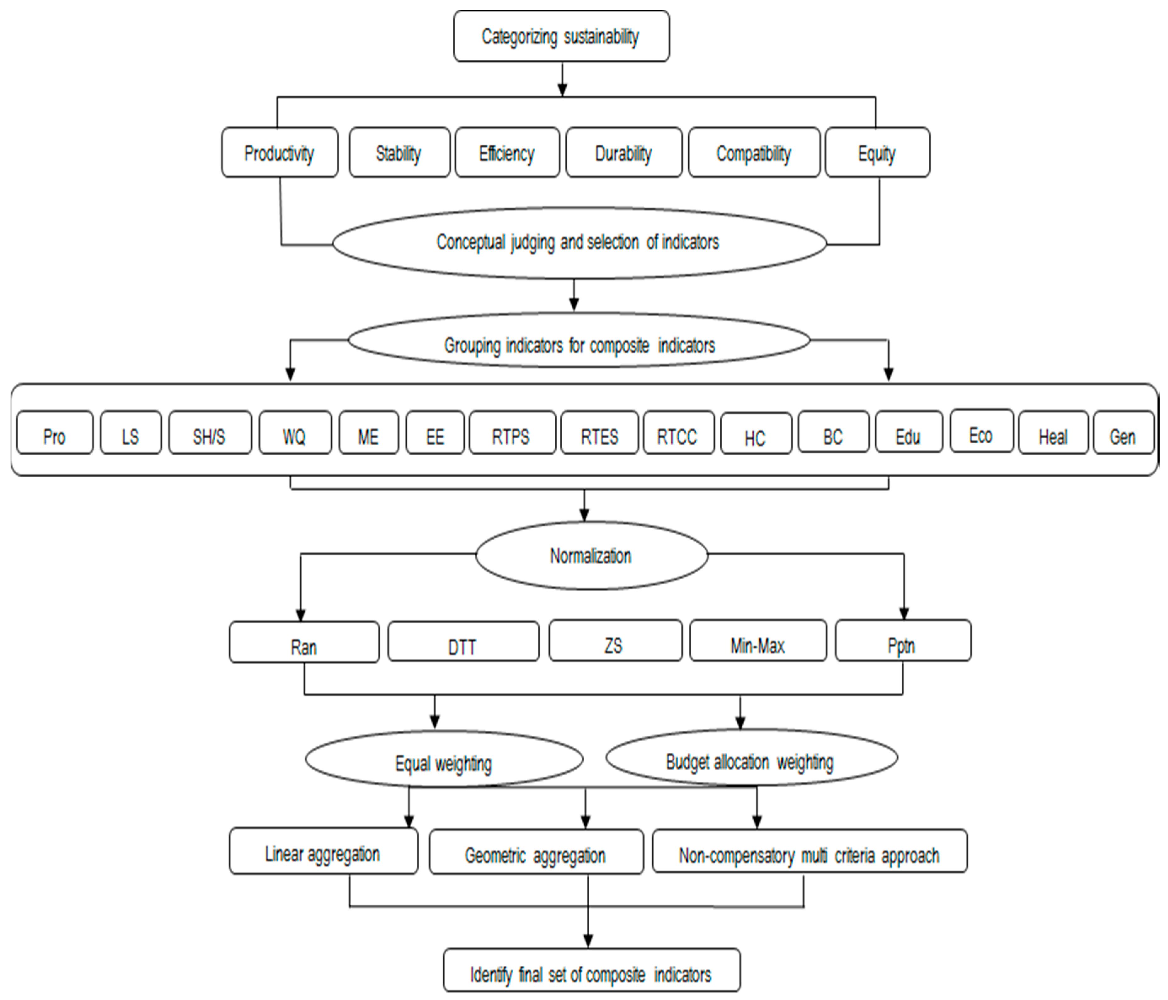

© 2017 by the authors. Licensee MDPI, Basel, Switzerland. This article is an open access article distributed under the terms and conditions of the Creative Commons Attribution (CC BY) license (http://creativecommons.org/licenses/by/4.0/).