Abstract
Accurate estimation of global horizontal irradiance (GHI) is essential for optimizing photovoltaic (PV) systems, particularly in regions with distinct climatic characteristics. Geostationary satellites, such as GK2A and COMS, provide consistent and spatially extensive data, offering a practical alternative to ground-based measurements. However, the performance of semi-empirical GHI models has been sparsely evaluated across diverse geographic zones. This study aimed to conduct a comparative analysis of four semi-empirical models—Beyer, Rigollier, Hammer, and Perez—applied to two contrasting locations: Seoul, South Korea (temperate) and Jakarta, Indonesia (tropical). Using satellite-derived cloud indices and ground-based pyranometer data, model performance was evaluated via RMSE, MBE, and their relative metrics. Results indicate that the Hammer model achieves the best performance in Seoul (RMSE: 103.92 W/m2; MBE: 0.09 W/m2), while the Perez model outperforms others in Jakarta with the lowest relative RMSE of 58.69%. The analysis outlines the limitations of transferring models calibrated in temperate climates to tropical settings without regional adaptation. This study provides critical insights for improving satellite-based GHI estimation and supports the development of region-specific forecasting tools essential for expanding solar infrastructure in Southeast Asia.
1. Introduction
The widespread adoption of solar photovoltaic (PV) energy represents a strong response to the challenges posed by global warming and climate change, primarily attributed to the combustion of fossil fuels. PV technology has further gained recognition as a leading form of sustainable energy, attributed to the inherent versatility and cost-effective maintenance. However, the intermittent nature of solar irradiance presents a significant hurdle, leading to unpredictability and variability in power generation from PV systems. This intermittency is intricately connected to regional climatic variables, including cloud cover, aerosol levels, and solar orientation specific to geographic locations. Consequently, the acquisition of precise solar irradiance data holds significant importance, as it maximizes solar PV power output and ensures the efficient operation of PV systems. Recognizing the potential of solar energy, governments worldwide, including those of South Korea and Indonesia, have implemented various initiastives to promote the adoption of PV technology. These efforts include incentive programs, subsidies, and policy frameworks aimed at encouraging investment in solar infrastructure and research and development, thereby advancing the transition to clean energy sources [1,2,3,4,5,6].
Making consistent progress in the collection of accurate and up-to-date solar irradiance data to address the difficulty of intermittent solar irradiance is necessary. To evaluate the viability of PV installations in a variety of geographical areas, having a solid understanding of local climate conditions is important. The all-inclusive comprehension makes it possible to accomplish better planning and management of PV systems, which maximizes the exploitation of solar resources. Furthermore, accurate measurements of solar irradiance offer several benefits, such as the ability to accurately anticipate the potential for energy generation, the optimization of system design and orientation, and the efficient operation of the system through real-time monitoring and adjustment. The incorporation of cutting-edge monitoring and forecasting technologies plays a significant role in minimizing the effects of intermittency, which leads to an improvement in the dependability and consistency of solar energy consumption. The necessity of gathering and using solar irradiance data is becoming more recognized by governments and research organizations worldwide, particularly in light of the ongoing improvements in solar PV technology [7,8,9].
The direct measurement of solar irradiance on the ground relies on specialized instruments such as pyranometers measuring total solar radiation and pyrheliometers evaluating direct solar radiation. These instruments are widely regarded as the most dependable sources of data. Significant advancements in irradiance measurement technology have recently facilitated the acquisition and automated monitoring of real-time data. Although ground measurement systems are reliable, the system still comes with substantial costs and requires meticulous maintenance. The spatial coverage area of ground measurements is also limited, and the existing measurement database falls short of meeting the demands of the modern PV industry. Despite efforts by some authors to mitigate the limitations of direct measurements’ spatial coverage through conventional methods such as interpolation, the accuracy of the interpolated data remains insufficient [7,10,11].
The use of satellite data is crucial in the precise monitoring of solar irradiance throughout the Earth’s surface. Zelenka et al. [7] outlined that the accuracy of data obtained from satellites was comparable to that gained through interpolation from a ground station located 25 km away. The integration of satellite-driven information into the national database is credited with the efficacy of the comprehensive coverage of solar radiation data in the United States [12]. Geostationary satellites, which are strategically connected with the Earth’s rotation, have exceptional capabilities in continually acquiring high-resolution imagery of precise regions on the Earth’s surface. The satellites in the most recent iteration have impressive spatial resolutions of 0.5 × 0.5 km for every visible channel image. For instance, Fengyun (Wind and Cloud)-4A (China Meteorological Administration, Beijing, China) and Geo-KOMPSAT-2A (GK2A) satellite systems (Korea Aerospace Research Institute, Daejeon, Republic of Korea) can provide 0.5 × 0.5 km spatial resolution, while the time interval is 15 and 10 min, respectively [13,14,15]. This signifies that the use of solar irradiance data obtained from geostationary satellite photos is a powerful and cost-effective solution for meeting the increasing needs of the solar energy industry.
The incorporation of remote sensing methods has presented substantial progress in both the time and location resolutions of data, facilitating the development of new and inventive methods for estimating solar irradiance. According to Kleissl [16], satellite-based solar irradiance models could be broadly classified into three primary categories namely physical, empirical, and semi-empirical methods. Physical methodologies primarily depend on radiative transfer models (RTMs) to thoroughly examine the transmission of radiation through different levels of the atmosphere. Comprehensive and precise data are necessary to provide reliable assessments of atmospheric constituents, including cloud optical properties, aerosol optical depth (AOD), and water vapor concentration [16]. In contrast, empirical models apply regression methods to create correlations between satellite measurements and ground-based records, relying exclusively on observable data [14]. Semi-empirical models provide a comprehensive integration of physical and empirical methods, facilitating the connection between theoretical comprehension and practical observations [17].
Many studies have made significant advancements in extracting satellite imagery for estimating global horizontal irradiance (GHI) [1,2,3,8,18,19,20,21,22,23]. As previously outlined, methods for estimating GHI are typically categorized as physical or semi-empirical. Physical models use RTMs to theoretically calculate the transmission of solar irradiance through the atmosphere. In contrast, semi-empirical models rely on empirical relationships between surface albedo and the clear-sky index, integrating key physical processes. Accurate simulation of these processes necessitates comprehensive atmospheric data, including AOD, ozone concentration, and precipitable water content. However, local atmospheric data availability often lags ground measurement data for solar irradiation. Semi-empirical models rely on simplified assumptions and statistical analysis [24]. The input variables used in semi-empirical models are generally more accessible compared to those used in physical models. A distinguishing aspect of semi-empirical models is the capability to forecast GHI for future periods [25]. Due to their simplicity and ease of implementation, semi-empirical models are favored for solar irradiance forecasting over physical models, which require more complex input data [15].
The effectiveness of semi-empirical models used to estimate solar irradiation has been investigated in several studies [2,3,8,18,20,21,22,26]. These studies have shown a wide range of discrepancies between the expected and observed radiation levels. A significant portion of the datasets used for developing and validating the models originates from countries situated within moderate latitudes, which share similarities with South Korea. Despite the increase, the application of semi-empirical models in South Korea remains rare. Moreover, when considering tropical environments, the scarcity of studies evaluating the efficacy of semi-empirical models is evens more pronounced.
Numerous studies conducted in South Korea have aimed to extract GHI data from the Communication, Ocean, and Meteorological Satellite (COMS) as well as the GK2A system in the country [25,26,27,28,29]. Since the development of COMS and GK2A, most studies have focused on physical models. Zo et al. [27] were the first to contribute to the field of GHI modeling of solar irradiance by using COMS data as input. The study also established the Gangneung-Wonju National University (GWNU) model, which was classified as a physical model. Kim et al. [28] estimated the solar irradiance over the Korean Peninsula by developing a physical model. The University of Arizona Solar Irradiance is based on the Korea Institute of Energy Research (KIER) satellite, called the UASIBS/KIER model. This model became the specific model to forecast solar irradiance in South Korea. Presently, Oh et al. [29] used the UASIBS/KIER model to forecast solar irradiance a few hours ahead. To the best of our knowledge, there are only a few studies that apply a semi-empirical method in the South Korean region. There are Kamil et al. [25] and Choi et al. [26] where Kamil et al. [25] conducted a comparison study between machine learning, physical, and semi-empirical models. A preprocessing method was integrated into the Rigollier model by Choi et al. [26] to distinguish between cloud cover and ground irradiance.
Several studies have been conducted in the tropical zone to quantify solar irradiance using semi-empirical methods and satellite systems [30,31,32,33]. However, there is a limited number of studies conducted on the analysis and modeling of solar radiation data specifically for the Southeast Asia region, which comprises Indonesia. As an example, Janjai [33] used Multifunction Transport Satellite-1 Replacement or Himawari-6 (MTSAT-1R, Japan Meteorological Agency, Tokyo, Japan) satellite data to make estimations of direct normal irradiance (DNI) at four distinct stations in Thailand. The study successfully obtained a relative root mean square error (rRMSE) value of 16%. The diffuse solar irradiance was assessed by Janjai et al. [34] using the Himawari 6 satellite system, yielding an rRMSE of 16.7%. Furthermore, a two-layered atmospheric model was developed by Janjai et al. [30] to estimate GHI over Thailand. The model achieved an rRMSE of approximately 10% as it is crucial to acknowledge the scarcity of publications that specifically examine the estimation of solar irradiance in Indonesia using satellite-based methods. Therefore, Sianturi et al. [35] examined the viability of using ECMWF reanalysis datasets and Modern-Era Retrospective Analysis for Research and Applications 2 (MERRA2, NASA Goddard Space Flight Center, Greenbelt, MD, USA) satellite data for the purpose of estimating solar irradiance in Indonesia. The methodology used in this study primarily consists of numerical weather prediction. The primary objective is to perform a comparative examination of semi-empirical models pertaining to satellite-derived global irradiance in Indonesia and South Korea.
The novelty of this work is rooted in four interrelated aspects that collectively advance the understanding of satellite-based solar irradiance estimation. First, this study provides one of the earliest systematic evaluations of semi-empirical models (Beyer, Rigollier, Hammer, and Perez) across two contrasting climatic regimes. It compares model performance in the temperate environment of Seoul, South Korea, and the tropical environment of Jakarta, Indonesia, offering new insights into their transferability and regional adaptability. Second, it integrates two generations of geostationary satellite data (COMS and GK2A) with ground-based pyranometer observations to ensure consistent radiometric calibration and enable a reliable cross-sensor and inter-annual comparison. Third, the study interprets model discrepancies not merely as statistical variations but as manifestations of distinct physical mechanisms such as differences in AOD, humidity, and cloud morphology, enhancing the physical interpretability of model performance. Fourth, it establishes a benchmark framework and reference dataset for adapting semi-empirical models to data-scarce tropical environments, laying the groundwork for future integration with machine learning and other data-driven methods. Collectively, the contributions define the scientific significance of this study and support the broader objectives of improving regional solar resource mapping and PV integration under diverse climatic conditions.
Considering the growing importance of semi-empirical models and the scarcity of relevant publications, this study aims to identify suitable semi-empirical models applicable to both the temperate climate of South Korea and the tropical climate of Indonesia. The overarching objective is to enrich the regional solar radiation database and facilitate the integration of PV systems into the local grid infrastructure. The primary objective is to conduct a comparative assessment of existing semi-empirical models for solar irradiance. The investigation will evaluate the accuracy of these models in estimating solar irradiance, specifically focusing on both South Korea and Indonesia. To achieve this, the Beyer [20], Rigollier [3], Hammer [18], and Perez [1] models have been chosen to generate hourly GHI data. These models will further be validated using ground measurements obtained from the Kookmin University station in Seoul and the Research and Development Center of the National Electricity State Corporation (Research and Development Center of the State Electricity Company) station in Jakarta, Indonesia. The performance of each model will be evaluated using error metrics such as RMSE, rRMSE, mean bias error (MBE), and relative mean bias error (rMBE).
2. Geostationary Imagery, Surface Monitoring, and Atmospheric Parameters
South Korea’s advancement in geostationary satellite technology started with the launch of the first meteorological satellite, COMS, in 2011, followed by the operational deployment of GK2A in 2018. Both satellites orbit at 128.2° E and were tasked with delivering continuous atmospheric and meteorological observations over a wide domain, including the Korean Peninsula, Southeast Asia, parts of China, and the Australian landmass. These satellite platforms were developed to strengthen early-warning capabilities for hazardous weather phenomena and to support long-term environmental monitoring. COMS was outfitted with multiple sensors, including a visible channel (0.67 µm), a water vapor channel (6.7 µm), and three thermal infrared bands (3.7 µm, 10.8 µm, and 12 µm), which were used for tracking cloud systems and surface characteristics. In contrast, GK2A incorporated a more advanced payload, such as the Advanced Meteorological Imager (AMI; Korea Aerospace Research Institute, Daejeon, Republic of Korea) which captured data across 16 spectral bands, allowing for detailed observation of atmospheric dynamics and climatic variability.
The GK2A’s visible channel imagery could be generated using four reflectance channels at wavelengths of 0.47 µm, 0.51 µm, 0.64 µm, and 0.86 µm. Additionally, it offered two near-infrared channels at wavelengths of 1.3 µm and 1.6 µm. The spectral spectrum, ranging from 3.8 µm to 13.3 µm was divided into 10 distinct infrared channels, each with core wavelengths, enabling detailed analysis of infrared radiation emitted from the Earth’s surface.
The spatial resolution of the visible channels differs between the COMS and GK2A satellites. COMS produced 16-bit visible images at 15-min intervals, with a spatial resolution of 1 × 1 km2 for the visible sensor and 4 × 4 km2 for its three infrared channels. In contrast, GK2A offered a higher spatial resolution of 0.5 × 0.5 km2 specifically for the 0.64 µm wavelength in its visible channels. For all infrared channels, including both near-infrared and shortwave infrared wavelengths, a spatial resolution of 2 × 2 km2 grid cells was used. The temporal resolution of GK2A showed improvement over COMS, with a scanning duration of approximately 10 min for complete disk images. As shown in Figure 1, the domain of GK2A comprised the entire geographical area of the Asia-Pacific Region. In this study, the cloud index (CI) extraction process included selecting a pixel from each image that closely matched the ground measurement for model validation. The datasets comprised hourly visible channel images from the COMS satellite covering the period from 1 January to 31 December 2018 (1 year), for South Korea. Meanwhile, visible images from GK2A were used for estimating solar irradiance over Indonesia from 1 January 2022 to 31 December 2022 (1 year). Although the COMS dataset (2018) and GK2A dataset (2022) corresponded to different years and sensor generations, both satellites shared identical orbital geometry (128.2° E) and underwent intercalibration by the National Meteorological Satellite Center. The normalization and cloud-index correction processes minimized radiometric differences between sensors. Therefore, the comparison was interpreted as a cross-climatic assessment rather than a strict sensor-to-sensor benchmark.
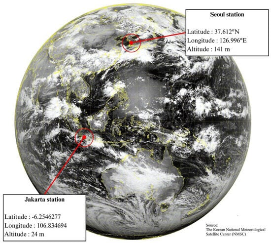
Figure 1.
Sample of visible satellite images (0.64 µm) were one of the channels provided by the GK2A satellite, which was stationed at 36,000 km above the equator. The image was considered as Level-1B full-disk data (https://datasvc.nmsc.kma.go.kr/datasvc/html/login/login.do; accessed on 12 June 2025).
This study included the measurement of GHI at two ground stations situated in distinct geographical regions, namely the northern part of Seoul (latitude: 37.612° N, longitude: 126.996° E, altitude: 141 m) and the central region of Jakarta (latitude: 6.254° S, longitude: 106.834° E, altitude: 24 m). GHI was quantified using a pyranometer (model MS-802), while DNI was gauged using a pyrheliometer (model MS-57). These instruments, manufactured by the EKO company in Japan, possessed a sensitivity of approximately ± 7 µVm2/W for both DNI and GHI measurements [36,37]. Ground-level data, such as satellite data, were stored locally at hourly intervals, comprising the time frames of 1 January to 31 December 2018, for South Korea, and 1 January 2022, to 31 December 2022, for Indonesia.
To minimize land-cover heterogeneity effects within the 1 × 1 km satellite pixel, the pixel whose center most closely overlapped the ground-station coordinates was selected for verification. Both ground stations were situated in dense urban environments, where local albedo and surface characteristics remained relatively homogeneous at this spatial scale. The Seoul site at Kookmin University represented an urban–vegetated campus setting surrounded by consistent built structures, while the Jakarta site was located at the PLN Research Institute in South Jakarta (6.254° S, 106.834° E). The auxiliary atmospheric parameters were obtained from the BMKG–Ancol AERONET station, approximately 10 km away, which was rooted within the typical 10–20 km aerosol decorrelation length for coastal–urban conditions. This proximity ensured the representativeness of aerosol and turbidity inputs used for semi-empirical modeling.
Before validating the model, ensuring that the ground measurement complied with the criteria for quality data was crucial. The study adopted criteria from Gueymard and Ruiz-Arias (2016) [38] to incorporate the specific parameters outlined to achieve the most favorable and rational value for ground measurement. The data must undergo the following conditions:
- 1.
- 2.
- 3.
where , , and represented the sun zenith angle, site elevation, and extraterrestrial irradiance on a normal surface, respectively. was specifically designed to exclude GHI results at low solar elevation. After all the necessary conditions have been met, an estimate of GHI was permitted using the nearest 1 × 1 km2 pixel to the ground measurement. Subsequently, the accuracy of the model was assessed.
The atmospheric data used by NASA were obtained from ground-based measurements obtained through the Aerosol Robotic Network (AERONET). Specifically, the open-access dataset was advantageous for numerous studies in the fields of meteorology and solar energy. The large datasets were created to aggregate atmospheric and weather datasets from diverse institutional networks located worldwide. Subsequently, these atmospheric data were made available to the public. The AERONET sun-sky radiometer system (Cimel Electronique CE-318, Paris, France) was tasked with collecting measurements of the solar spectrum across eight distinct spectral bands, namely 340, 380, 440, 500, 675, 870, 940, and 1020 nm, covering a broad range of wavelengths. Acknowledging that the calibration, post-processing, and standardization procedures were required for all datasets collected by AERONET was important. These large datasets comprised AOD, ozone, nitrogen concentration, and precipitable water , optical thickness, Angstrom wavelength exponent , Angstrom turbidity , and well pressure . The AERONET datasets were obtained from the Yonsei University site (≈8 km from Kookmin University, Seoul) and the BMKG–Ancol site (≈10 km from PLN Research Institute, Jakarta). Both sites were located within the typical 10–20 km aerosol decorrelation length of urban–coastal environments. The BMKG–Ancol station was also the only open-access AERONET site currently operational in the Jakarta region, making it the sole available source for atmospheric parameterization. Although this introduced minor spatial limitations, the prevailing wind systems and standardized AERONET calibration procedures ensured that the data remained representative for semi-empirical model inputs. The AERONET data collection consisted of three primary levels, namely level 1, which comprised unprocessed data; level 1.5, including data that had been devoid of clouds; and level 2, corresponding to quality-controlled data. This study used and extrapolated AERONET level 1.5 data into hourly intervals. The analysis adopted only the AERONET dataset, which specifically spanned 12 months and included measurements of GHI, COMS, and GK2A satellite images. The datasets used in this study, including measurements of GHI, COMS, and GK2A satellite images, are summarized in Table 1.

Table 1.
List of datasets used in this work.
3. Methodology
This study adopted several well-established semi-empirical models to estimate GHI in two distinct locations, namely Seoul and Jakarta. The selection of models, including Beyer, Rigollier, Hammer, and Perez, was based on historical use, documented accuracy, and adaptability across geographic contexts. Initially developed using Meteosat satellite data, these models have undergone validation primarily in European environments.
The Beyer model [20] evolved from the Heliosat-1 framework and incorporated refinements such as geometric corrections, backscatter adjustments, and clear-sky irradiance calculations. It delivered hourly GHI estimates with a root mean square error (RMSE) around 120 Wh/m2, translating to a relative RMSE (rRMSE) of approximately 16%. Rigollier [3] further advanced the Heliosat-1 method by replacing raw digital values with calibrated radiance inputs, thereby enabling a more physically grounded estimation of irradiance. For validation, the model yielded RMSEs and rRMSEs of 62 Wh/m2 (45%) in January 1995, 96 Wh/m2 (27%) in April 1995, and 103 Wh/m2 (18%) in July 1994.
Hammer’s model [18] focused on near-term forecasting by generating motion vector fields from consecutive satellite images to simulate cloud movement. These vectors were then projected forward in time, typically up to two hours and in 30-min intervals, enabling short-range GHI predictions. The forecast rRMSE values were reported as 35% for 1-h and 40% for 2-h horizons. In contrast, the Perez model [1] was originally calibrated using data from the GOES satellite system over the Americas. It was validated using ten ground stations spread across diverse climate zones, yielding RMSEs in the range of 44 to 118 W/m2 depending on location.
In this study, four semi-empirical models, namely Beyer, Rigollier, Hammer, and Perez, were selected to estimate GHI because of their methodological diversity, prior validation, and relevance across both temperate and tropical regions. The Beyer model served as a simplified reference framework based on geometric and radiative adjustments. In contrast, the Rigollier model integrated physically grounded parameters, including atmospheric turbidity and calibrated radiance, which enhanced its performance under diverse aerosol and humidity conditions. The Hammer model, initially designed for short-term irradiance forecasting using cloud-motion vectors, was adapted in this study for diagnostic purposes to ensure methodological consistency with the other methods. In this mode, it reconstructed instantaneous GHI from current satellite imagery without performing temporal extrapolation of cloud fields. The Perez model, validated across multiple climates using GOES satellite data, applied explicit corrections for solar geometry and air mass (AM), making it broadly adaptable. Collectively, these models spanned a continuum of complexity and input requirements, enabling a comprehensive comparison of the performance under the distinct climatic regimes of Seoul and Jakarta.
3.1. Satellite Radiance Correction and CI Derivation
GHI from satellite data included a multistep process that integrated geometric correction, atmospheric adjustment, and cloud classification. An overview of this workflow was shown in Figure 2, which outlined how raw satellite imagery and auxiliary atmospheric parameters were processed through normalization and CI estimation to produce surface-level irradiance estimates. This schematic reflected the shared foundation of the four semi-empirical models implemented in this study, despite the differing correction methodologies.
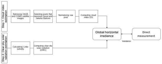
Figure 2.
Procedure to derive solar irradiance from GK2A satellite images.
In satellite-based solar irradiance estimation, surface reflectance recorded by visible imagery must be adjusted to account for geometric and atmospheric distortion. Raw pixel values from satellite sensors were not directly comparable due to influences such as solar position, sensor viewing angle, and scattering effects. Therefore, normalization was a foundational preprocessing step, correlating image-derived values with physically interpretable metrics.
Semi-empirical models addressed these challenges using correction schemes customized to each model’s assumptions and input requirements. Raw reflectance values were converted into normalized pixel intensities using geometric and atmospheric corrections. These corrections ensured that satellite-derived brightness values were consistent with physical radiative transfer processes under clear-sky conditions.
A critical geometric factor affecting image brightness was AM, which described the effective atmospheric path length traversed by incoming solar radiation. When the sun was low on the horizon, sunlight passed through a longer atmospheric column, increasing scattering and absorption. The backscattering effect further complicated reflectance measurements, especially when the satellite and solar viewing angles were closely correlated, producing an apparent enhancement in surface albedo—known as the “hot-spot” effect. These distortions were most pronounced near sunrise and sunset and must be accounted for to ensure reliable irradiance estimation.
To mitigate these influences, both the Beyer and Hammer models implemented correction coefficients derived from the satellite zenith angle , , and backscattering angle . The extraterrestrial irradiance , adjusted by the sun–Earth distance factor , was used to scale the normalized value. These inputs corrected for solar geometry and variability in Earth–Sun distance throughout the year, which affected the irradiance reaching the top of the atmosphere.
In contrast, the Rigollier model integrated radiative transfer-based corrections using the European Solar Radiation Atlas (ESRA) methodology. It introduced transmittance terms for both downward and upward atmospheric paths—denoted as and , and accounted for atmospheric turbidity through the Linke turbidity factor (TL). The model also incorporated a correction term for clear-sky diffuse irradiance and sensor-specific irradiance response , calculated by integrating the radiometer’s spectral sensitivity function over the solar spectrum. These parameters enabled the model to account for aerosol content and atmospheric scattering more precisely.
The Perez model used a distinct method by using the Sun’s elevation angle and AM directly in its normalization formulation. In contrast to other models that emphasized geometric corrections or empirical radiative fits, Perez integrated observational statistics from multi-year satellite archives to derive dynamic normalization bounds. Although this offerred greater generalizability across sites, the analysis confined the model to a single-year dataset and do not incorporate long-term tuning of the backscatter envelope.
After pixel normalization was completed, cloud presence was quantified through the CI, which expressed how much a given pixel deviates from its theoretical clear-sky value. The CI was computed as a linear transformation between the minimum called and maximum normalized reflectance thresholds, representing clear-sky and fully overcast conditions, respectively.
The normalization formulas corresponding to each semi-empirical model, which form the basis for computing the CI as expressed in Equation (1), are summarized in Table 2. Following Strategy 4 proposed by Chen et al. (2022) [17], the upper and lower limits of the normalized reflectance were determined on a fixed monthly basis. The upper bound was defined as the mean of the ten highest reflectance values, and the lower bound as the mean of the second to fifth lowest values. This method improved robustness against outliers, avoided artificial temporal drift, and ensured seasonally consistent bounds for CI estimation.
Table 2.
Pixel normalization formula for obtaining an independent CI (step 2). Each ‘raw’ pixel was subjected to this normalization before extracting the CI.
CI values typically ranged from 0 (no cloud) to 1 (full cloud cover), but values might exceed the range under conditions such as cloud edge enhancement or high-albedo surfaces such as snow. The accuracy of CI classification was contingent upon the robustness of the pixel normalization process. Previous studies [2,3,18,20] have established empirically derived bounds for and , depending on satellite characteristics and regional atmospheric conditions.
In summary, each semi-empirical model adopted a personal pixel correction scheme based on distinct assumptions such as geometric adjustment (Beyer, Hammer), transmittance and turbidity fitting (Rigollier), or empirical solar geometry calibration (Perez). These corrections were necessary to ensure that CI values and GHI estimates were physically meaningful and regionally transferable.
3.2. Clear-Sky Irradiance and Turbidity Factor
An essential aspect of semi-empirical models was the determination of the maximum level of solar irradiance, known as the clear-sky irradiance . The reduction in solar irradiance under clear skies was dependent on the abundance of absorbers and scatterers in the atmosphere, such as aerosols, gases, and water vapor. The primary emphasis of most clear-sky models was rooted in the mitigation of solar radiation caused by atmospheric components and the geometric correlation of the sun. The clear-sky irradiance model was less complex than the semi-empirical method because it accounted for the rapid changes in aerosols, water vapor, and other molecules. A well-known turbidity index, known as Linke Turbidity , could be derived by combining various atmospheric variables [39,40,41].
This study explored the application of four semi-empirical models, each model adopting unique procedures for calculating GHIC. The Beyer model adopted a straightforward clear-sky model based on geometric calculations. Specifically, the model used here, known as the Bourges clear-sky formula, exclusively uses the parameter to represent the reduction in extraterrestrial solar irradiance as it traversed through the Earth’s atmosphere. Derived from an empirical correlation between ground measurements, sun position, and site location, this model provided a simplified portrayal of clear-sky conditions.
Conversely, the Rigollier model, also referred to as the ESRA model, divided clear-sky irradiance into direct and diffuse components, incorporating and the Rayleigh scattering factor . The clear-sky irradiance formula of the Hammer model closely resembled that of the Rigollier model. Although both models shared identical formulations for clear-sky Direct Normal Irradiance (DNIC) equations, the equations for clear-sky Diffuse Horizontal Irradiance (DHIC) differed.
The Linke turbidity was a crucial parameter in clear-sky modeling, capturing atmospheric conditions’ impact. served as a crucial measure for quantifying atmospheric attenuation due to absorption and scattering. It could be evaluated using either a direct or indirect formula [42]. The direct formula, also known as the pyrheliometric formula, typically incorporated measurements of DNI, optical AM, and the . Conversely, the indirect, or parameterized formula, integrated atmospheric constituents such as AM, , angstrom turbidity factor , and AOD. Following extensive testing of various TL formulas, the model proposed by Remund et al. [43], particularly Equation (10), was identified as the most suitable and was hence used for this study.
The clear-sky irradiance formulations corresponding to each semi-empirical model, including Beyer, Rigollier, Hammer, and Perez, are comprehensively summarized in Table 3, which consolidates the equations and key parameters applied to derive surface irradiance under clear-sky conditions.
Table 3.
Clear-sky irradiance formulas based on semi-empirical model.
3.3. GHI Conversion and Error Metrics Formulation
After CI and GHIC were considered, GHI was performed from GHIC by appropriately reducing according to CI. The reduction factor was called the clear sky index , and was expressed as a correlation function. Finally, the conversion equations were summarized in Table 4.
Table 4.
GHI conversion based on semi-empirical models, which consider .
To evaluate the difference between projected values and observed measurements, establishing metrics that measured accuracy was crucial. The metric known as the RMSE was adopted to evaluate the degree of dispersion in forecasts compared to the actual measurements. The MBE was commonly used as a method for evaluating whether a model showed positive bias (overestimation) or negative (underestimation) in relation to a long-term average. When the values of RMSE, rRMSE, MBE, and rMBE approached zero, an estimation model was considered to be of high quality.
4. Results
The input parameters for all semi-empirical models in estimating solar irradiance over Jakarta and Seoul are represented in Table 5. Among the models, the Beyer model stood out for its simplicity and minimal reliance on the TL factor in atmospheric conditions. However, when assessing versatility and comprehensiveness, the Rigollier and Hammer models evolved as the preferred choices. These models allowed for the simultaneous calculation of three components, namely GHI, DNI, and DHI under clear sky conditions. These results were validated across significant regions of Europe and Africa, which included regions with a similar climate to South Korea. Rigollier and Hammer models were rare in tropical areas, and even fewer were in Indonesia. With the array of input variables, the Perez model appeared promising for potential implementation in both South Korea and Indonesia. The Perez model incorporated an implicit variable, , and based on Perez et al. [44], it underwent dynamic changes instead of remaining constant throughout the year. Consequently, the process of selecting was considered an independent variable.
Table 5.
Comparison of input variables in semi-empirical models. “✓” symbol indicates that the corresponding input variable is included in the model formulation.
Figure 3 and Figure 4 showed the graphical depiction of the variations in GHIC as a function of Sun elevation in both Seoul and Jakarta. In general, it was evident that all the models showed similar trends, as the levels of GHIC suggested a positive correlation with Sun elevation . Each model further yielded different dispersions due to the underlying formula. The Beyer model did not include atmospheric conditions in the TL, as previously stated. The Beyer model results showed the lowest magnitude of dispersion compared to the others. The Rigollier and Hammer models showed a similar pattern, with the Hammer model signifying slightly higher levels of dispersion. On the contrary, a significant level of dispersion was observed in both the Perez and the remaining three groups. Acknowledging that the existence of either a minor or significant dispersion did not necessarily imply that the GHIC exhibited a significant degree of precision was necessary. However, TL had a significant impact on both of these models. The models showed variability in the upper and lower limits of GHIC values. For instance, the Beyer model yielded the smallest values in two locations. In Seoul Station, it showed GHIC between 70.22 W/m2 and 859.54 W/m2. Meanwhile, Jakarta stations presented GHIC around 131.43 W/m2 and 997.54 W/m2. The Hammer model produced a broader range of values, 50.78–1092.52 W/m2 and 116.63–1032.90 W/m2 for Seoul and Jakarta, respectively. On the other hand, the Perez model estimated GHIC between 5.86–998.23 W/m2 and 48.56–1048.80 W/m2 over Seoul and Jakarta, respectively. The Rigollier model showed the most elevated GHIC values, which varied between 108.65 W/m2 and 1055 W/m2.
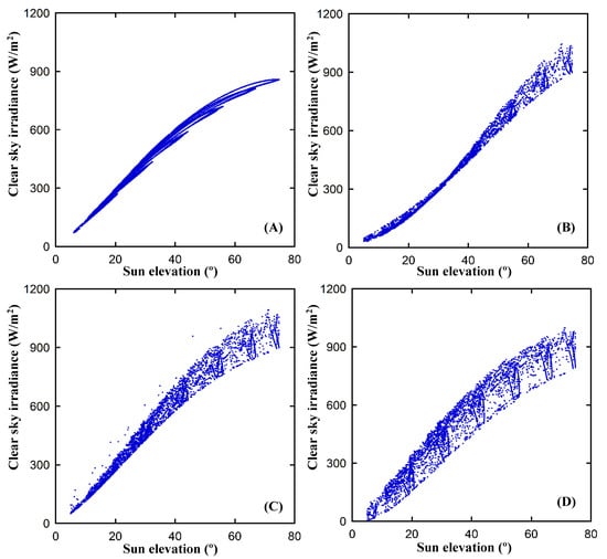
Figure 3.
Estimated clear-sky GHI (W/m2) as a function of solar elevation angle (°) over Seoul, South Korea, using the Beyer (A), Hammer (B), Perez (C), and Rigollier (D) models. The blue points represent the estimated clear-sky irradiance values simulated by each semi-empirical model as a function of sun elevation.
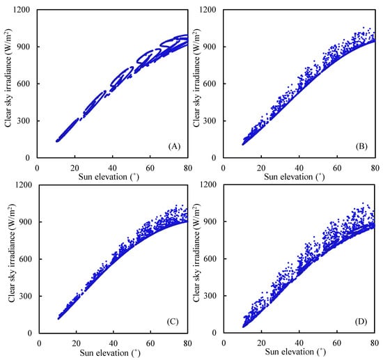
Figure 4.
Estimated clear-sky GHI (W/m2) as a function of solar elevation angle (°) over Jakarta, Indonesia, using the Beyer (A), Hammer (B), Perez (C), and Rigollier (D) models. The blue points represent the estimated clear-sky irradiance values simulated by each semi-empirical model as a function of sun elevation.
The normalization of pixels was a critical step in the computation of CI, as it allowed for the consideration of backscatter and AM effects, which often introduced bias in images. Therefore, the procedure of normalization facilitated the precise assessment of the true luminosity of the Earth’s surface. The digital numerical range for COMS and GK2A pixels, respectively, spanned from 0 to 1024 and 0 to 16,000. Figure 5 and Figure 6 presented scatterplots that visually represented the pixel values after the normalization process had been applied to each model. The expectation was that the normalized pixels would show a uniform dynamic range, including both the upper and lower limits. In all of the models that were analyzed, the lower boundary showed a relatively uniform pattern, except for cases where the backscatter angles were low. To provide further clarification, it was observed that as the backscatter angle approached 0°, signifying the satellite’s proximity to the sun, there was a propensity for the lower boundary to show a marginal augmentation. The minimum value showed that there had been no significant alteration in the Earth’s surface albedo. It was also expected that the upper limits, which were indicative of overcast weather conditions, would remain constant. The upper boundaries showed a higher degree of variability in magnitude when compared to the lower counterparts. Moreover, there were occurrences of significantly elevated values, comprising a small number of outliers that surpassed the upper limit. The process of establishing the upper limits was marked by heightened levels of uncertainty, leading to a reduction in the precision of GHI estimation under overcast circumstances. The Beyer model exhibited significant disparities in both the interquartile range and the maximum value, distinguishing it from the other three models. The determination of the CI was derived from the range of the normalized pixel counts, as shown in Figure 5 and Figure 6. The calculation was performed using Equation (1). Therefore, the term “CI” referred to a measure of attenuation that was calculated based on the clear-sky global horizontal irradiance (GHIC).
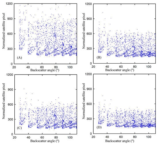
Figure 5.
Normalized satellite values from COMS plotted against backscatter angle (°) for the Seoul site. (A–D) are Beyer, Hammer, Perez, and Rigollier models. The upper and lower radiometric bounds ( and ) were determined using the fixed-monthly Strategy 4 of Chen et al. (2022) [17]. The typical monthly range was and . Original COMS digital counts (0–1024) were normalized before CI derivation. The blue dotted points represent the normalized satellite reflectance values plotted as a function of backscatter angle for each semi-empirical model.
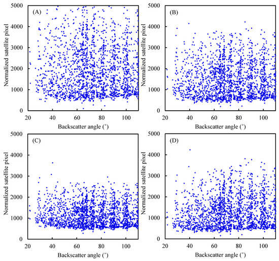
Figure 6.
Normalized Satellite values from GK2A plotted against backscatter angle (°) for the Jakarta site. (A–D) are Beyer, Hammer, Perez, and Rigollier models. The upper and lower radiometric bounds ( and ) were determined using the fixed-monthly Strategy 4 of Chen et al. (2022) [17]. Typical monthly range are and . Original GK2A digital counts (0–16,000) were normalized before CI derivation. The blue dotted points represent the normalized satellite reflectance values plotted as a function of backscatter angle for each semi-empirical model.
The term “accuracy for all sky conditions” implied the overall performance observed across the period from 2018 and 2022 in Seoul and Jakarta, respectively. The models generated varied results, with none exceeding 62.93% for rRMSE and 14.88% for rMBE, as shown in Figure 7 and Figure 8, as well as summarized in Table 6 and Table 7.
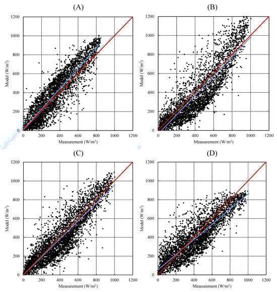
Figure 7.
Comparison between modeled and measured GHI under all-sky conditions at the Seoul site. Panels (A–D) represent the Beyer, Rigollier, Hammer, and Perez models, respectively. The red line shows the 1:1 reference (perfect agreement), while the blue line shows the linear regression between modeled and measured GHI. Legends provide RMSE and MBE values (W m−2) for each model. Both axes are expressed in (W m−2).
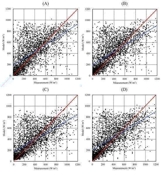
Figure 8.
Comparison between modeled and measured GHI under all-sky conditions at the Jakarta site. Panels (A–D) represent the Beyer, Rigollier, Hammer, and Perez models. The red line denoted the 1:1 reference, and the blue line represented the best-fit regression. Legends included RMSE and MBE values (W m−2) for each model. Axes were standardized in W m−2 to enable direct comparison among models.
Table 6.
The validation of GHI models under all-sky conditions in the year 2018, Seoul, South Korea. (n = 4037 hourly samples after QC, 2018).
Table 7.
The validation of GHI models under all-sky conditions in the year 2022, Jakarta, Indonesia. (n = 3222 hourly samples after QC, 2022).
The Hammer model showed superior performance in Seoul compared to the other three semi-empirical models, achieving the highest agreement in terms of RMSE and MBE calculations, with values of 103.92 W/m2 and 0.09 W/m2, respectively. Although the Hammer model showed superior performance in Seoul, the disparities in accuracy among the Hammer, Perez, and Beyer models were statistically insignificant. The difference in rRMSE between the Hammer and Perez models was a mere 2.1%, while the difference between the Hammer and Beyers models was a mere 2.64%. On the other hand, the Rigollier model showed the highest level of error, as evidenced by an MBE value of −36.84 W/m2.
The study results showed that the Perez model exhibited superior performance compared to the other three semi-empirical models in Jakarta. This was evident in the Perez model’s ability to achieve the highest level of agreement in terms of RMSE and MBE, with values of 212.08 W/m2 and 16.46 W/m2, respectively. Despite the Perez model’s superior performance, the differences in accuracy between the Rigollier, Hammer, and Beyer models were minimal. The variation in rRMSE between the Perez and Hammer models was a mere 3.24%, while the difference between the Perez and Beyer models was modest at 4.24%. In contrast, the Rigollier model showed the highest level of error, with an MBE value of 53.77 W/m2. Formal uncertainty estimation (e.g., bootstrap resampling or paired statistical tests) was not performed, as the models shared identical datasets and exhibited strong temporal autocorrelation, violating independence assumptions. Considering the one-year hourly dataset size (>8000 samples), the sampling uncertainty was negligible compared to systematic model bias. Therefore, the ranking of models was interpreted based on consistent error trends rather than probabilistic intervals.
When comparing GHI at the Jakarta station to the Seoul location, there was a discernible discrepancy in the accuracy of semi-empirical models, as the accuracy of these models was lower in Indonesia. There were several possible explanations for this disparity. First, the Beyer, Hammer, Perez, and Rigollier models were initially developed for climates in Europe and America. Due to the precise location, the coefficients and linear regressions that were built into these models were largely consistent with areas such as Europe and the USA, which were very different from Indonesia’s tropical climate. Second, a major factor affecting model accuracy was the geographical separation between the Jakarta Station and the AERONET station. The AERONET datasets may not accurately reflect the ground-based GHI conditions at the Seoul Station, even though both stations were in Jakarta. Significantly, there were significant differences in cloudiness, pollution, atmospheric density, and radiation between the AERONET station, close to the beach, and the Jakarta station located in an urban area. The variations led to a decreased degree of accuracy, but instead of seeing the difficulties as failures, this work opened a range of possibilities for future publication directions. Three interesting avenues for further publications were identified. This study focused on all-sky conditions to maintain consistency between regions and ensure sufficient data density across the annual cycle. Although stratified evaluations (clear, broken, and overcast) could show condition-specific strengths of each semi-empirical model, the limited sample sizes for individual categories could reduce statistical robustness. Future publications should incorporate stratified analysis once multi-year datasets become available, particularly to examine the models’ behavior under low-sun and heavy-cloud regimes.
5. Discussion
Creating a specific semi-empirical model for tropical areas has become an essential aspect. To ensure a more accurate representation of solar irradiance in these regions, the formulation of such a model should consider the distinct climatic characteristics of Southeast Asia and Indonesia. In addition to modifying current models, this strategy investigates a cutting-edge method that considers the complex interactions between elements unique to tropical climates.
The differing performance of the Hammer and Perez models can be attributed to the contrasting atmospheric and climatic regimes of Seoul and Jakarta. Seoul’s temperate environment is dominated by layered stratiform clouds, moderate humidity, and strong seasonal variations in aerosol loading—conditions that enhance the radiometric stability of visible-band satellite observations. Under these circumstances, the Hammer model, which relies on geometric normalization and cloud-motion corrections, effectively captures gradual radiance changes connected to aerosol backscatter and synoptic cloud evolution. In contrast, Jakarta’s tropical climate is characterized by persistent convective activity, high precipitable-water content, and rapid transitions between clear and overcast conditions. These factors increase diffuse irradiance and cause stronger short-term variability in cloud optical thickness. The Perez model’s empirical transmittance formulation, which integrates air-mass and solar-geometry corrections, is better suited to such high-humidity, convective atmospheres, as it smooths short-lived fluctuations in cloud albedo and moisture-induced scattering. Consequently, the model performs more robustly under tropical conditions where diffuse radiation dominates.
Acknowledging that the datasets for South Korea and Indonesia correspond to different years—2018 and 2022, respectively, is crucial. This temporal difference may introduce minor inter-annual variability in atmospheric conditions such as cloud fraction, aerosol loading, and seasonal humidity. However, the purpose of this study is not a year-to-year climatological comparison but a cross-climatic evaluation between temperate and tropical regimes. Both datasets were acquired from geostationary satellites positioned at the same orbital longitude (128.2° E) and radiometrically cross-calibrated by the National Meteorological Satellite Center (NMSC), ensuring consistency in viewing geometry and sensor response. Moreover, the analysis emphasizes relative model performance metrics (RMSE, MBE, rRMSE, rMBE) rather than absolute irradiance values, thereby minimizing the influence of year-specific weather anomalies. Although subtle differences connected to large-scale events such as ENSO or aerosol fluctuations cannot be completely excluded, these effects are secondary to the main objective of assessing how each semi-empirical model behaves under contrasting climatic environments.
This study also acknowledges a spatial limitation arising from the use of only one validation site per country—Seoul in South Korea and Jakarta in Indonesia. Although both stations are representative of highly urbanized and coastal settings typical of their respective climates, they do not capture the full spectrum of regional and topographical diversity present within each nation. For example, South Korea exhibits marked variability between its southern coastal regions and northern continental zones, while Indonesia’s vast archipelagic landscape introduces large gradients in humidity, cloud morphology, and aerosol content. Therefore, the results presented here should be interpreted as indicative of model transferability across contrasting climatic regimes rather than a comprehensive national assessment. Future studies should incorporate additional validation sites, including inland, high-altitude, and coastal locations, to enhance spatial representativeness and recalibrate model parameters for diverse sub-climatic environments. Establishing a network of coordinated pyranometers and AERONET stations would provide a valuable foundation for these expanded analyses.
In addition to spatial representativeness, another key limitation arises from the transferability of semi-empirical models originally developed in European mid-latitude contexts. These models were calibrated using radiative coefficients and atmospheric assumptions specific to temperate conditions, such as moderate humidity, stratiform cloud cover, and relatively stable AOD. In contrast, tropical regions such as Indonesia experience higher convective cloud frequency, greater water-vapor variability, and non-linear aerosol–humidity interactions. These physical differences alter the relationship between normalized satellite radiance and surface irradiance, reducing the accuracy of models when directly applied without regional recalibration. Accordingly, the limitation is primarily physical rather than methodological, emphasizing the need for region-specific parameterization of radiative transfer and turbidity terms to ensure robust GHI estimation in tropical atmospheres.
A second alternative is to strategically install a network of GHI and atmospheric measurement instruments throughout different parts of Indonesia. The wide-ranging network not only makes it easier to improve the accuracy of the model, but it also provides strong validation because it takes into consideration the various atmospheric conditions found in various parts of the nation. In practice, the design of such a network should be regionally adaptive. For relatively homogeneous lowland regions, such as the northern coast of Java, a station spacing of approximately 50–100 km would be sufficient to capture mesoscale atmospheric variability and support satellite calibration. In contrast, in mountainous or topographically intricate areas—such as the West Java highlands or eastern archipelagic zones—a denser spacing of 20–30 km is recommended to account for localized cloud formation and elevation effects. The inclusion of urban–rural station pairs would further help quantify the influence of aerosols, albedo, and urban heat on irradiance. Each major climatic zone should ideally host at least one reference-grade site equipped with a pyranometer, sun photometer, and auxiliary atmospheric sensors, complemented by secondary low-cost instruments for continuity. This hierarchical configuration follows the World Meteorological Organization network recommendations and would significantly enhance model calibration and regional irradiance monitoring in Indonesia. The creation of a network of such measurement sites can provide useful information for enhancing and verifying solar irradiance models, enhancing the capacity for prediction.
Beyond traditional modeling, semi-empirical methods retain strategic importance where high-quality vertical atmospheric data and dense surface observations are limited. Compared with radiative-transfer models, the frameworks require fewer parameters while maintaining physical interpretability through variables such as AM and turbidity. In contrast, data-driven models, including machine learning and deep learning, excel at capturing complex non-linear relationships but demand extensive, high-frequency training datasets. This trade-off makes semi-empirical methods particularly valuable as baseline tools in data-scarce tropical regions like Indonesia, where satellite observations are abundant, but ground monitoring networks remain sparse.
Accordingly, the present study provides a baseline performance benchmark for semi-empirical models across contrasting climates, defining an accuracy envelope that future hybrid frameworks can refine. A promising roadmap includes coupling semi-empirical outputs (e.g., clear-sky or cloud-index estimates) with adaptive machine learning correction layers that learn residual biases, integrate uncertainty, and dynamically adjust model coefficients. This hybrid paradigm merges the physical stability of semi-empirical formulations with the adaptive learning capacity of machine learning systems—offering a scalable and interpretable method for solar forecasting under tropical atmospheric variability.
To complement the statistical evaluation of model accuracy, Figure 9 presents the spatial distribution of estimated GHI across South Korea and Indonesia during August 2022. This map was generated using the best-performing semi-empirical models identified for each region (Hammer for Seoul and Perez for Jakarta) applied to satellite imagery. August was selected as it represents a typical high-radiation month in both hemispheres, showing the model’s ability to capture solar energy potential under favorable sky conditions. It should be asserted that the GHI map in Figure 9 was generated for August 2022 using GK2A imagery for both countries. This representation was included solely to show regional irradiance patterns under comparable seasonal conditions and did not replace the 2018 COMS-based validation for Seoul. Because GK2A was radiometrically cross-calibrated with COMS by KMA/NMSC, the 2022 spatial results remained physically consistent with the 2018 dataset.
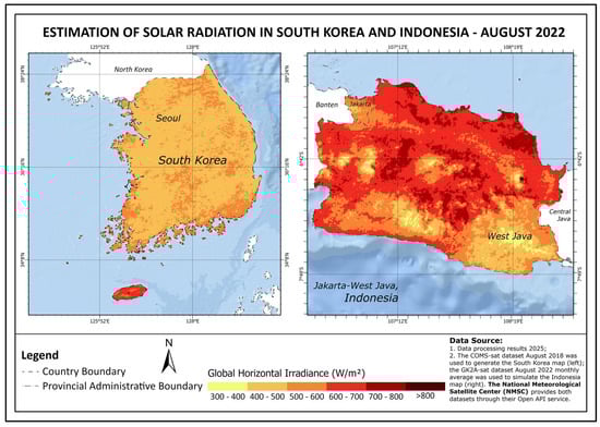
Figure 9.
Spatial distribution of estimated global horizontal irradiance (GHI, W/m2) over South Korea (left, using GK2A data) and Indonesia (right, Jakarta and West Java) for August 2022. This figure serves an illustrative purpose to visualize spatial patterns during a representative high-irradiance month; the formal model validation for Seoul was performed using 2018 COMS data. The COMS satellite dataset August 2018 monthly average was used to create the South Korea map, while the GK2A satellite dataset August 2022 monthly average was used to simulate the Indonesian map. The National Meteorological Satellite Center (NMSC, accessed on 12 June 2025) which provided both datasets via the Open API service.
The GHI map outlines significant spatial variability across both countries. In South Korea, irradiance levels generally range between 500–700 W/m2, with coastal and southern regions receiving higher solar input. Conversely, in Indonesia, particularly across West Java, spatial variability is more pronounced, with irradiance exceeding 800 W/m2 in many inland regions. These spatial patterns are influenced by cloud dynamics, elevation, aerosol concentrations, and land cover differences. The inclusion of this spatial product not only reinforces the model’s applicability but also underscores the necessity for high-resolution solar mapping in future infrastructure and grid integration planning.
6. Conclusions
In conclusion, this study conducted a comparative evaluation of four semi-empirical models, namely Perez, Hammer, Beyer, and Rigollier, for estimating GHI, using geostationary satellite data from COMS (2018 dataset) and GK2A (2022 dataset). The assessment was performed in two contrasting climatic zones, namely the tropical urban area of Jakarta and the temperate metropolitan region of Seoul. Across both locations, the models generally tended to overestimate GHI, particularly in Jakarta, where the Maximum Bias Error (MBE) remained below 53.77 W/m2. Among the models tested, the Beyer model showed the highest RMSE in Jakarta, suggesting relatively poor performance under humid tropical atmospheric conditions. In contrast, the Rigollier model yielded the lowest predictive accuracy in Seoul, with RMSE values reaching a minimum of 35.09 W/m2.
Based on RMSE, relative RMSE (rRMSE), MBE, and relative MBE (rMBE), the Hammer model evolved as the most reliable for temperate climates such as Seoul. The Perez model further showed relatively better performance in Jakarta, suggesting its adaptability to tropical environments. These results pointed to the geographically contingent performance of semi-empirical models, which were often calibrated using datasets and atmospheric assumptions derived from European or North American contexts.
Importantly, the study underscored the limitations of transferring models across climatic zones without proper revalidation or recalibration. The disparity in model performance between Jakarta and Seoul was a direct reflection of differences in cloud dynamics, humidity levels, aerosol concentration, and seasonal solar geometry. Consequently, there was an urgent need to develop or adapt semi-empirical models specifically tailored for tropical climates, where conventional models may fail to capture the high variability and convective cloud cover typical of equatorial regions.
To address these limitations, future publications should prioritize the establishment and expansion of ground-based solar monitoring networks across Indonesia to support more robust validation efforts. Furthermore, integrating data-driven methods, particularly machine learning algorithms, could enhance prediction accuracy by dynamically learning complex atmospheric interactions that static models may overlook. In the long term, a hybrid framework that combined semi-empirical modeling with machine learning optimization offered a scalable solution for real-time solar forecasting in tropical environments, supporting the deployment of solar energy infrastructure under Indonesia’s diverse climatic conditions.
Author Contributions
P.M.P.G.: Conceptualization, Formal Analysis, Investigation, Methodology, Project Administration, Resources, Software, Supervision, Validation, Visualization, Writing—Original Draft, and Editing. R.O.A.: Data Curation, Formal Analysis, Investigation, Methodology, Software, Visualization, and Draft Writing. H.L.: Conceptualization, Software, and Validation. I.A.A.: Data Curation, Formal Analysis, Investigation, and Methodology. R.D.D.: Writing—Review and Editing, Validation, Visualization, and Supervision. I.S.S.: Writing—Review and Editing, and Validation. R.R.: Data Curation, Formal Analysis, and Validation. I.G.: Conceptualization, Supervision, Draft Writing—Review and Editing. J.T.S.S.: Conceptualization, Validation, Writing—Review and Editing. M.D.: Conceptualization, Funding Acquisition, Resources, Investigation, Methodology, Writing—Review and Editing, Visualization, and Supervision. All authors have read and agreed to the published version of the manuscript.
Funding
This study is supported by funds from HIBAH PUTI Q1 2024–2025 of DRPM UI University of Indonesia (NKB-420/UN2.RST/HKP.05.00/2024) and the National Research Foundation of Korea (NRF), Ministry of Science and ICT (2023R1A2C1004663).
Data Availability Statement
The data and other study materials that support the results of this study were obtained from the internal repositories of the Department of Geography, Faculty of Mathematics and Natural Sciences, Universitas Indonesia; the Indonesian Agency for Meteorology, Climatology, and Geophysics (BMKG), and the Department of Mechanical Engineering, Kookmin University, Seoul, South Korea. The data are available to the public upon request. Satellite datasets used in this study were obtained from publicly available archives of the National Meteorological Satellite Center (NMSC), Korea Meteorological Administration (KMA). COMS Level-1B visible imagery (0.67 µm) for 2018 and GK2A Level-1B visible imagery (0.64 µm) for 2022 were accessed through the open-API request portal at https://nmsc.kma.go.kr. Ground-based irradiance measurements for Seoul were collected at the Kookmin University Station (37.612° N, 126.996° E) using an EKO MS-802 pyranometer, and for Jakarta at the PLN Research Institute Station (6.254° S, 106.834° E) using the same instrument model. Atmospheric auxiliary parameters were derived from the AERONET Level 1.5 datasets—Yonsei University site for Seoul and BMKG–Ancol site for Jakarta—covering January–December 2018 and January–December 2022, respectively. The processing scripts for cloud-index (CI), clear-sky index (kₐ), and clear-sky irradiance (GHIC) conversions were developed in MATLAB (version 2022A) and Python (version 3.12) using standard image-processing and numerical libraries. These routines are available from the corresponding author upon reasonable request for academic and non-commercial study purposes.
Acknowledgments
The authors also thank: (1) the Department of Geography, Faculty of Mathematics and Natural Sciences, Universitas Indonesia; (2) the Indonesian Agency for Meteorology, Climatology, and Geophysics (BMKG); (3) the Department of Mechanical Engineering, Kookmin University, Seoul, Korea, for providing data from the study’s inception to its conclusion; (4) Perusahaan Listrik Negara (PLN) Research Institute for providing fruitful discussions, dataset, and technical insights; and (5) the editor and reviewers for the constructive feedback.
Conflicts of Interest
The authors declare no conflicts of interest.
Nomenclature
The following abbreviations are used in this manuscript:
| AOD | Aerosol optical depth |
| Normalized maximum satellite pixel value | |
| Normalized minimum satellite pixel value | |
| Raw satellite pixel value | |
| Normalized actual satellite pixel value | |
| Extraterrestrial irradiance on a normal surface (W/m2) | |
| The extraterrestrial irradiance (W/m2) | |
| Total irradiance in the visible sensor of the satellite system (W/m2) | |
| Clear-sky index | |
| Atmospheric path transmittance from the sun to the Earth’s surface | |
| P | Atmospheric pressure |
| TL | Linke Turbidity Factor |
| Atmospheric path transmittance from the Earth’s surface to the visible sensor of the satellite | |
| W | Precipitable water vapor |
| z | Site elevation (m) |
| Greek Symbols | |
| Anstrom wavelength exponent | |
| Anstrom turbidity | |
| Sun zenithal angle (°) | |
| Satellite zenith angle (°) | |
| Backscattering angle (°) | |
| the sun–Earth distance factor | |
| Sun elevation angle | |
| Rayleigh scattering factor | |
| Abbreviations | |
| AERONET | Aerosol Robotic Networks |
| AM | Air mass |
| CI | Cloud index |
| COMS | Communication Ocean and Meteorological Satellite |
| DHI | All-sky diffuse horizontal irradiance (W/m2) |
| DHIC | Clear-sky diffuse horizontal irradiance (W/m2) |
| DNI | All-sky direct normal irradiance (W/m2) |
| DNIC | Clear-sky direct normal irradiance (W/m2) |
| GHI | All-sky global horizontal irradiance (W/m2) |
| GHIC | Clear-sky global horizontal irradiance (W/m2) |
| KMA | Korean Meteorological Administration |
| MBE | Mean bias error (W/m2) |
| NASA | National Aeronautics and Space Administration |
| NMSC | National Meteorological Satellite Center |
| RMSE | Root Mean Square Error (W/m2) |
| rRMSE | Relative root mean square error (W/m2) |
| rMBE | Relative mean bias error % |
References
- Ineichen, P.; Perez, R. Derivation of cloud index from geostationary satellites and application to the production of solar irradiance and daylight illuminance data. Theor. Appl. Climatol. 1999, 64, 119–130. [Google Scholar] [CrossRef]
- Perez, R.; Ineichen, P.; Moore, K.; Kmiecik, M.; Chain, C.; George, R.; Vignola, F. A new operational model for satellite-derived irradiances: Description and validation. Sol. Energy 2002, 73, 307–317. [Google Scholar] [CrossRef]
- Rigollier, C.; Lefèvre, M.; Wald, L. The method Heliosat-2 for deriving shortwave solar radiation from satellite images. Sol. Energy 2004, 77, 159–169. [Google Scholar] [CrossRef]
- Yang, D.; Wang, W.; Gueymard, C.A.; Hong, T.; Kleissl, J.; Huang, J.; Perez, M.J.; Perez, R.; Bright, J.M.; Xia, X.; et al. A review of solar forecasting, its dependence on atmospheric sciences and implications for grid integration: Towards carbon neutrality. Renew. Sustain. Energy Rev. 2022, 161, 112348. [Google Scholar] [CrossRef]
- Madsuha, A.F.; Setiawan, E.A.; Wibowo, N.; Habiburrahman, M.; Nurcahyo, R.; Sumaedi, S. Mapping 30 years of sustainability of solar energy research in developing countries: Indonesia case. Sustainability 2021, 13, 11415. [Google Scholar] [CrossRef]
- Kennedy, S.F. Indonesia’s energy transition and its contradictions: Emerging geographies of energy and finance. Energy Res. Soc. Sci. 2018, 41, 230–237. [Google Scholar] [CrossRef]
- Zelenka, A.; Perez, R.; Seals, R.; Renné, D.; Renne, D. Effective accuracy of satellite-derived hourly irradiances. Theor. Appl. Climatol. 1999, 62, 199–207. [Google Scholar] [CrossRef]
- Mouhamet, D.; Tommy, A.; Primerose, A.; Laurent, L. Improving the Heliosat-2 method for surface solar irradiation estimation under cloudy sky areas. Sol. Energy 2018, 169, 565–576. [Google Scholar] [CrossRef]
- Benbba, R.; Barhdadi, M.; Ficarella, A.; Manente, G.; Romano, M.P.; El Hachemi, N.; Barhdadi, A.; Al-Salaymeh, A.; Outzourhit, A. Solar Energy Resource and Power Generation in Morocco: Current Situation, Potential, and Future Perspective. Resources 2024, 13, 140. [Google Scholar] [CrossRef]
- Yagli, G.M.; Yang, D.; Gandhi, O.; Srinivasan, D. Can we justify producing univariate machine-learning forecasts with satellite-derived solar irradiance? Appl. Energy 2020, 259, 114122. [Google Scholar] [CrossRef]
- Ŝúri, M.; Hofierka, J. A new GIS-based solar radiation model and its application to photovoltaic assessments. Trans. GIS 2004, 8, 175–190. [Google Scholar] [CrossRef]
- National Renewable Energy Laboratory. National Solar Radiation Database 1991–2005 Update: User’s Manual; Task No. PVA7.6102; National Renewable Energy Laboratory: Golden, CO, USA, 2007. [Google Scholar] [CrossRef]
- Duan, J.; Zuo, H.; Bai, Y.; Chang, M.; Chen, X.; Wang, W.; Ma, L.; Chen, B. A multistep short-term solar radiation forecasting model using fully convolutional neural networks and chaotic aquila optimization combining WRF-Solar model results. Energy 2023, 271, 126980. [Google Scholar] [CrossRef]
- Chen, S.; Li, C.; Xie, Y.; Li, M. Global and direct solar irradiance estimation using deep learning and selected spectral satellite images. Appl. Energy 2023, 352, 121979. [Google Scholar] [CrossRef]
- Garniwa, P.M.P.; Rajagukguk, R.A.; Kamil, R.; Lee, H.J. Intraday forecast of global horizontal irradiance using optical flow method and long short-term memory model. Sol. Energy 2023, 252, 234–251. [Google Scholar] [CrossRef]
- Kleissl, J. Solar Energy Forecasting and Resource Assessment; Academic Press: Cambridge, MA, USA, 2013. [Google Scholar] [CrossRef]
- Chen, S.; Liang, Z.; Guo, S.; Li, M. Estimation of high-resolution solar irradiance data using optimized semi-empirical satellite method and GOES-16 imagery. Sol. Energy 2022, 241, 404–415. [Google Scholar] [CrossRef]
- Hammer, A.; Heinemann, D.; Hoyer, C.; Kuhlemann, R.; Lorenz, E.; Müller, R.; Beyer, H.G. Solar energy assessment using remote sensing technologies. Remote Sens. Environ. 2003, 86, 423–432. [Google Scholar] [CrossRef]
- Cano, D.; Monget, J.M.; Albuisson, M.; Guillard, H.; Regas, N.; Wald, L. A method for the determination of the global solar radiation from meteorological satellite data. Sol. Energy 1986, 37, 31–39. [Google Scholar] [CrossRef]
- Beyer, H.G.; Costanzo, C.; Heinemann, D. Modifications of the heliosat procedure for irradiance estimates from satellite images. Sol. Energy 1996, 56, 207–212. [Google Scholar] [CrossRef]
- Moradi, I.; Mueller, R.; Alijani, B.; Kamali, G.A. Evaluation of the Heliosat-II method using daily irradiation data for four stations in Iran. Sol. Energy 2009, 83, 150–156. [Google Scholar] [CrossRef]
- Eissa, Y.; Chiesa, M.; Ghedira, H. Assessment and recalibration of the Heliosat-2 method in global horizontal irradiance modeling over the desert environment of the UAE. Sol. Energy 2012, 86, 1816–1825. [Google Scholar] [CrossRef]
- Meflah, A.; Chekired, F.; Drir, N.; Canale, L. Accurate method for Solar Power Generation Estimation for different PV (photovoltaic panels) technologies. Resources 2024, 13, 166. [Google Scholar] [CrossRef]
- Garniwa, P.M.P.; Ramadhan, R.A.A.; Lee, H.J. Application of semi-empirical models based on satellite images for estimating solar irradiance in Korea. Appl. Sci. 2021, 11, 3445. [Google Scholar] [CrossRef]
- Kamil, R.; Garniwa, P.M.; Lee, H.J. Performance assessment of global horizontal irradiance models in all-sky conditions. Energies 2021, 14, 7939. [Google Scholar] [CrossRef]
- Seok, C.W.; Ram, S.A.; Yong, K. Solar irradiance estimation in Korea by using modified heliosat-II method and COMS-MI imagery. J. Korean Soc. Surv. Geod. Photogramm. Cartogr. 2015, 33, 463–472. [Google Scholar] [CrossRef]
- Zo, I.S.; Jee, J.B.; Lee, K.T.; Kim, B.Y. Analysis of solar radiation on the surface estimated from GWNU solar radiation model with temporal resolution of satellite cloud fraction. Asia-Pac. J. Atmos. Sci. 2016, 52, 405–412. [Google Scholar] [CrossRef]
- Kim, C.K.; Kim, H.G.; Kang, Y.H.; Yun, C.Y. Toward Improved Solar Irradiance Forecasts: Comparison of the Global Horizontal Irradiances Derived from the COMS Satellite Imagery Over the Korean Peninsula. Pure Appl. Geophys. 2017, 174, 2773–2792. [Google Scholar] [CrossRef]
- Oh, M.; Kim, C.K.; Kim, B.; Yun, C.; Kang, Y.H.; Kim, H.G. Spatiotemporal optimization for short-term solar forecasting based on satellite imagery. Energies 2021, 14, 2216. [Google Scholar] [CrossRef]
- Janjai, S.; Pankaew, P.; Laksanaboonsong, J. A model for calculating hourly global solar radiation from satellite data in the tropics. Appl. Energy 2009, 86, 1450–1457. [Google Scholar] [CrossRef]
- Janjai, S.; Sricharoen, K.; Pattarapanitchai, S. Semi-empirical models for the estimation of clear sky solar global and direct normal irradiances in the tropics. Appl. Energy 2011, 88, 4749–4755. [Google Scholar] [CrossRef]
- Janjai, S.; Masiri, I.; Laksanaboonsong, J. Satellite-derived solar resource maps for Myanmar. Renew. Energy 2013, 53, 132–140. [Google Scholar] [CrossRef]
- Janjai, S. A method for estimating direct normal solar irradiation from satellite data for a tropical environment. Sol. Energy 2010, 84, 1685–1695. [Google Scholar] [CrossRef]
- Charuchittipan, D.; Choosri, P.; Janjai, S.; Buntoung, S.; Nunez, M.; Thongrasmee, W. A semi-empirical model for estimating diffuse solar near infrared radiation in Thailand using ground- and satellite-based data for mapping applications. Renew. Energy 2018, 117, 175–183. [Google Scholar] [CrossRef]
- Sianturi, Y.; Marjuki; Sartika, K. Evaluation of ERA5 and MERRA2 reanalyses to estimate solar irradiance using ground observations over Indonesia region. AIP Conf. Proc. 2020, 2223, 020002. [Google Scholar] [CrossRef]
- EKO Instrument Co., Ltd. MS-802 Instruction Manual Pyranometer Ver. 3; Version 3; EKO Instrument Co., Ltd.: Tokyo, Japan, 2019. [Google Scholar]
- EKO Instrument Co., Ltd. MS-57 Instruction Manual Pyrheliometer Ver. 3; Version 3; EKO Instrument Co., Ltd.: Tokyo, Japan, 2019. [Google Scholar]
- Gueymard, C.A.; Ruiz-Arias, J.A. Extensive worldwide validation and climate sensitivity analysis of direct irradiance predictions from 1-min global irradiance. Sol. Energy 2016, 128, 1–30. [Google Scholar] [CrossRef]
- Eltbaakh, Y.A.; Ruslan, M.H.; Alghoul, M.A.; Othman, M.Y.; Sopian, K.; Razykov, T.M. Solar attenuation by aerosols: An overview. Renew. Sustain. Energy Rev. 2012, 16, 4264–4276. [Google Scholar] [CrossRef]
- Song, A.; Choi, K.; Jung, M.; Kim, Y. Estimation of the Linke turbidity factor and the solar irradiance under a clear sky over the Korean Peninsula using COMS MI. New Renew. Energy 2016, 12, 21. [Google Scholar] [CrossRef]
- Marif, Y.; Bechki, D.; Zerrouki, M.; Belhadj, M.M.; Bouguettaia, H.; Benmoussa, H. Estimation of atmospheric turbidity over Adrar city in Algeria. J. King Saud Univ. 2019, 31, 143–149. [Google Scholar] [CrossRef]
- Garniwa, P.M.P.; Lee, H. Intercomparison of the parameterized Linke turbidity factor in deriving global horizontal irradiance. Renew. Energy 2023, 212, 285–298. [Google Scholar] [CrossRef]
- Remund, J.; Wald, L.; Lefèvre, M.; Ranchin, T.; Page, J. Worldwide Linke turbidity information. ISES Sol. World Congr. 2003 2003, 400, 13. [Google Scholar] [CrossRef]
- Hanrieder, N.; Sengupta, M.; Xie, Y.; Wilbert, S.; Pitz-Paal, R. Modeling beam attenuation in solar tower plants using common DNI measurements. Sol. Energy 2016, 129, 244–255. [Google Scholar] [CrossRef]
Disclaimer/Publisher’s Note: The statements, opinions and data contained in all publications are solely those of the individual author(s) and contributor(s) and not of MDPI and/or the editor(s). MDPI and/or the editor(s) disclaim responsibility for any injury to people or property resulting from any ideas, methods, instructions or products referred to in the content. |
© 2025 by the authors. Licensee MDPI, Basel, Switzerland. This article is an open access article distributed under the terms and conditions of the Creative Commons Attribution (CC BY) license (https://creativecommons.org/licenses/by/4.0/).