Spatially Gated Mixture of Experts for Missing Data Imputation in Pavement Management Systems

Abstract

Accurate imputation of missing pavement-condition data is critical for proactive infrastructure management, yet it is complicated by spatial non-stationarity—deterioration patterns and data quality vary markedly across regions. This study proposes a Spatially Gated Mixture-of-Experts (SG-MoE) imputation model that explicitly encodes spatial heterogeneity by (i) clustering road segments using geographic coordinates and (ii) supervising a gating network to route each sample to region-specialized expert regressors. Using a large-scale national pavement management database, we benchmark SG-MoE against a strong baseline under controlled missingness mechanisms (MCAR: missing completely at random; MAR: missing at random; MNAR: missing not at random) and missing rates (10–50%). Across scenarios, SG-MoE consistently matches or improves upon the baseline; the largest gains occur under MCAR and the challenging MNAR setting, where spatial specialization reduces systematic underestimation of high crack-rate sections. The results provide practical guidance on when spatially aware ensembling is most beneficial for infrastructure imputation at scale. We additionally report comparative results under three missingness mechanisms. Across five random seeds, SG-MoE is comparable to the single LightGBM baseline under MCAR/MAR and achieves its largest gains under MNAR (e.g., sMAPE improves by 0.82 points at 10% MNAR missingness).

1. Introduction

Road infrastructure deteriorates inevitably under traffic loads and environmental stresses, making timely maintenance essential for safety and cost-effectiveness [1,2]. Pavement management systems rely on periodic condition surveys that measure indicators of road damage, such as crack rate, surface roughness (flatness), and rutting depth, to identify distress and prioritize repairs [3,4]. Accurate and up-to-date data on these metrics is critical for guiding maintenance decisions in a timely manner [5,6]. However, ensuring high-quality road condition data at a national scale is challenging, as large databases often suffer from errors, inconsistencies, and missing entries [7].

Advances in sensing and data collection have partially automated the gathering of pavement condition data [8,9]. Specialized survey vehicles equipped with cameras and lasers now capture road surface images and profile measurements, yielding data on cracking, plastic deformation (rutting), and longitudinal smoothness [10,11]. For example, a recent nationwide survey in South Korea investigated the crack rate, deformation, and roughness of 38,000 lane kilometers of national road [12]. While such automation greatly increases data coverage, human involvement is still required for data processing and input. Field inspectors and engineers must validate and integrate survey results, and in practice many agencies continue to rely on manual or semi-automated data entry procedures [8,9,13]. This mix of automated collection with manual handling can introduce data quality issues including transcription errors, inconsistent formatting, and, notably, gaps where no valid data is recorded [14]. The sheer volume of information now collected (far beyond what personnel can realistically review) makes it infeasible to correct all errors by hand. As a result, missing data in pavement condition databases is common [15]. Traditionally, engineers have managed missing values by either discarding incomplete records or applying rudimentary imputation (e.g., using interpolation, mean values, or regression estimates). These ad hoc solutions, however, may undermine data integrity and bias subsequent pavement performance analysis.

Fortunately, road condition data exhibit strong spatial patterns that present an opportunity for more intelligent data imputation [16]. Continuous road segments in close proximity tend to experience similar traffic loads, construction histories, and climatic conditions, leading to correlated deterioration rates among neighboring sections [17]. In other words, if one road section’s measured crack rate or rut depth is missing or unreliable, the conditions of adjacent segments (with known data) can provide informative clues [16]. Infrastructure researchers have long recognized that incorporating spatial dependency can improve pavement modeling. For example, dividing a highway network into homogeneous sections by region or climate can account for broad spatial trends [18]. In pavement deterioration modeling, it has been suggested that a section’s future condition could be better predicted by considering the condition of nearby sections exposed to the same environment and loads [19]. Spatial continuity is thus a valuable signal for inferring missing pavement data [20,21]. However, previous attempts to exploit spatial characteristics in pavement data analysis have been limited in scope and success [22]. Simple spatial interpolation or regional averaging often fails to capture fine-grained dependencies in the road network, and such methods do not fully leverage the complex interactions between neighboring road segments [23]. In practice, many pavement management systems still lack a robust mechanism to harness spatial information when dealing with missing data, leaving a significant gap in data quality improvement efforts [24].

The main contributions of this study are as follows: (i) we formulate large-scale crack-rate imputation as a spatially non-stationary learning problem and introduce SG-MoE to explicitly model regional heterogeneity through supervised spatial gating; (ii) we provide implementation details that make SG-MoE practical for multi-million-row pavement databases by combining a lightweight gating MLP with scalable tree-based experts; (iii) we conduct a controlled and reproducible evaluation under MCAR (Missing Completely At Random), MAR (Missing At Random), MNAR(Missing Not at Random) mechanisms at multiple missing rates, reporting both accuracy metrics and statistical tests; and (iv) we discuss failure modes under extreme MNAR missingness and outline concrete improvement strategies for future work.

The remainder of this paper is organized as follows. Section 2 reviews related work on missing-data imputation and pavement condition modeling. Section 3 presents the proposed SG-MoE framework, including the gating function, training objective, and evaluation protocol. Section 4 reports experimental results and analysis across missingness scenarios. Section 5 concludes with implications for pavement management and future research directions.

2. Related Works

2.1. Conventional Imputation Methods

Early approaches to missing data imputation rely on simple statistical strategies [25]. Mean or median imputation replaces a missing entry with the mean or median of observed values, providing a quick but potentially biased fix [26]. Regression imputation uses a predictive model (often linear regression) to estimate missing values from other features, capturing some relationships at the expense of assuming a functional form [27]. Nearest-neighbor methods (KNN) have also been widely used, where a missing value is filled by a weighted average of the values from the most similar k instances. This leverages local similarity but can struggle if nearest neighbors are distant in feature space [28,29,30]. Another widely adopted strategy is Multiple Imputation by Chained Equations (MICE), an iterative method that fits a series of regression models to impute each variable in turn and repeats this process multiple times to account for uncertainty. MICE is popular for its flexibility with different variable types and its ability to generate multiple plausible imputations for robust statistical inference [31]. These traditional techniques are straightforward and often effective for small or independent and identically distributed datasets, but they typically treat samples independently and ignore any spatial or complex dependency structure in the data [26,30]. Moreover, simplistic methods (mean, single regression) tend to underestimate variability, while even iterative approaches like MICE assume the data’s missingness mechanisms (e.g., Missing At Random) and may perform poorly if those assumptions are violated [32].

2.2. Machine Learning Based Imputation

As datasets become more complex, machine learning methods that capture nonlinear patterns and perform imputation have emerged. Ensemble tree models, particularly random forests, form the basis of the MissForest algorithm [33]. MissForest iteratively trains a random forest regression model for each missing feature, using other features as predictors, and has demonstrated excellent performance even on mixed data types [34]. Similarly, gradient boosting trees (e.g., XGBoost-based imputation) have been applied to directly predict missing values or integrated into various imputation frameworks to leverage high predictive accuracy. While these tree-based methods can model complex interactions, they operate sample-by-sample, essentially neglecting spatial relationships [35]. Another direction of development is the use of matrix factorization and low-rank models, which assume the underlying low-dimensional structure of the data (as in collaborative filtering) and can fill in missing values through matrix completion techniques. These methods (e.g., soft imputation, SVD-based imputation) are effective when global latent structure exists, but can ignore local spatial nuances [36,37]. Over the past decade, deep learning techniques have been increasingly applied to imputation. Denoising autoencoders (DAEs) effectively learn context and replace missing values by learning compressed data representations that can reconstruct inputs with missing values [38]. Stacked denoising autoencoders and other neural network architectures have outperformed many existing methods by capturing nonlinear correlations among features [39]. Likewise, variational autoencoders (VAE) and generative adversarial networks (GAN) have been adapted for imputation [40]. Yoon et al. (2018) [41] introduced the Generative Adversarial Imputation Network (GAIN), which uses a GAN to generate plausible values conditioned on observed data. Such models learn the joint distribution of data to sample realistic imputations and have shown advantages in creating coherent imputations that respect complex feature relationships. However, these deep models, including Recurrent Neural Network-based methods for time-series gaps (e.g., Bidirectional Recurrent Imputation for Time Series, Gated Recurrent Unit-D), generally handle data as if each sample (or each time series) is independent [42,43]. They excel at temporal or feature-wise dependency modeling but do not inherently consider spatial dependency. The fact that observations in close spatial proximity or along a network may be correlated. This limitation means that purely non-spatial machine learning imputations can perform suboptimally on geo-referenced data, where location-based autocorrelation is a key feature of the missingness structure.

3. Methodology

3.1. Overall Framework

The proposed methodology adopts a MoE framework specifically tailored for the crack-rate imputation problem, with an emphasis on modeling spatial heterogeneity in pavement conditions.

Figure 1 summarizes the workflow adopted in this study. Starting from the raw PMS (Pavement Management System) database, we apply standard preprocessing steps, including feature construction and variable transformation, and then perform spatial clustering to divide the road network into several geographically coherent clusters. Based on these cluster-wise datasets, we induce missing values according to the predefined MCAR, MAR, and MNAR mechanisms, thereby creating controlled training scenarios for each cluster. The imputation models are trained on these data using a composite objective that combines the mean squared error for the target crack-rate variable with a cross-entropy term that regularizes the gating function. Finally, the models are evaluated by comparing the imputed values with the ground truth, and the resulting error metrics are used to quantify imputation performance across clusters and missingness scenarios.

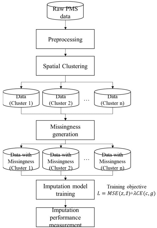
Figure 1. Overall experimental framework for training and evaluating the imputation models.

Figure 2 presents an overview of the overall architecture. Instead of relying on a single, globally trained model, we employ an ensemble of specialized expert models whose contributions are adaptively weighted by a gating network. For each road segment, the gating mechanism determines the most relevant expert(s) based on the segment’s spatial and contextual features. The underlying intuition is that pavement deterioration patterns, particularly crack formation, vary substantially across geographic regions due to factors such as climate, traffic load, and maintenance practices. Hence, a spatially aware ensemble can more accurately estimate missing crack-rate values than a uniform global model.

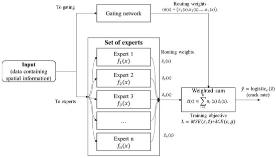
Figure 2. Spatially Gated MoE architecture.

To facilitate stable and effective model training, we first performed feature engineering and data normalization. Each road segment is represented by features vector $\mathrm{x}$ including repair quantities, roughness indices, curvature and an observed crack rate $\mathrm{y}$ (percentage, 0 to 100%). we apply a logit transformation to map it to an unbounded continuous domain

$$\mathrm{z}={\mathrm{l}\mathrm{o}\mathrm{g}\mathrm{i}\mathrm{t}}_{\mathrm{ϵ}}\left(\mathrm{y}\right)=\log \left({\displaystyle \frac{\mathrm{y}+\mathrm{ϵ}}{1-\left(\mathrm{y}+\mathrm{ϵ}\right)}}\right),\mathrm{ϵ}={10}^{-6}$$

(1)

where a small constant $\mathrm{ϵ}={10}^{-6}$ ensures numerical stability. This transformation allows regression models to predict in the real-valued space. At inference time, the predicted value is transformed back to the original scale through the inverse logistic function below.

$$\widehat{\mathrm{y}}=\mathrm{l}\mathrm{o}\mathrm{g}\mathrm{i}\mathrm{s}\mathrm{t}\mathrm{i}{\mathrm{c}}_{\mathrm{ϵ}}\left(\widehat{\mathrm{z}}\right)={\displaystyle \frac{1}{1+\exp \left(-\widehat{\mathrm{z}}\right)}}-\mathrm{ϵ}$$

(2)

To capture additional domain-specific information, we construct an intensity feature by aggregating the patching and repair areas and applying a logarithmic transformation to reduce skewness ($\mathrm{i}\mathrm{n}\mathrm{t}\mathrm{e}\mathrm{n}\mathrm{s}\mathrm{i}\mathrm{t}\mathrm{y}=\mathrm{l}\mathrm{o}\mathrm{g}(1+\mathrm{a}\mathrm{r}\mathrm{e}\mathrm{a})$).

Categorical identifiers (e.g., route ID, survey ID) are encoded via target encoding, embedding the historical mean crack rate of each category. Cross-validation is used in this encoding process to prevent data leakage. Continuous features with missing values (e.g., roughness, rutting depth) are imputed using their median values, ensuring a complete feature matrix for all experts.

To incorporate geographic context, we partition the road segments into $\mathrm{K}$ spatial clusters (regions) using their latitude and longitude coordinates. In this study, we set $\mathrm{K}=5$ obtained via K-Means clustering on the latitude and longitude pairs, resulting in five distinct spatial regimes. These regimes serve as prior indicators of spatial variation in crack-rate behavior. Instead of training separate models for each cluster, which could introduce data scarcity and discontinuities at boundaries, we use these clusters to guide $\mathcal{L}$ within a unified MoE framework. This strategy provides a balance between regional specialization and global consistency, enabling smooth transitions across geographic boundaries.

The core component of the proposed framework is the Spatially Gated Mixture-of-Experts model. It consists of two components: (1) a gating network that outputs a weight or responsibility ${\mathrm{\alpha }}_{\mathrm{i}}$ for each expert $\mathrm{i}$ based on the input features, and (2) a set of $\mathrm{K}$ expert models ${\mathrm{f}}_1,{\mathrm{f}}_2$, $\dots$, ${\mathrm{f}}_{\mathrm{K}}$ that each predict the crack rate (in logit space) for a given input. The gating network is trained to learn the mapping from a segment’s features $\mathrm{f}\left(\mathrm{x}\right)$ to a probability distribution over the $\mathrm{K}$ spatial clusters, effectively answering “which spatial regime does this segment most likely belong to?”. Each expert model is specialized to a particular regime or pattern in the data; during training, each expert primarily uses data from the segments that belong to its regime (as determined by the gating function). By combining their predictions with the gating weights, the MoE can adapt its output to different conditions: for instance, one expert may become specialized in high-curvature mountain roads while another specializes in flat highways, and for a new segment the model will automatically give more influence to the appropriate expert based on that segment’s characteristics.

During the imputation process, each data instance (road segment) passed through the gating network to obtain a set of weights ${\mathrm{\alpha }}_1, \dots , {\mathrm{\alpha }}_{\mathrm{K}}$, and simultaneously obtain predictions from all expert models. The final crack rate estimate is a weighted mixture of the experts’ outputs. The gating weights act like attention scores telling us how much to trust each expert. For an instance with feature vector $\mathrm{f}\left(\mathrm{x}\right)$, if ${\mathrm{z}}_{\mathrm{i}}={\mathrm{f}}_{\mathrm{i}}$(x) is expert i’s predicted crack logit, then the MoE’s combined prediction in logit space is ${\mathrm{z}}_{\mathrm{m}\mathrm{i}\mathrm{x}}= \sum _{\mathrm{i}=1}^{\mathrm{K}}{\mathrm{\alpha }}_{\mathrm{i}}\left(\mathrm{x}\right){\mathrm{z}}_{\mathrm{i}}$. This ${\mathrm{z}}_{\mathrm{m}\mathrm{i}\mathrm{x}}$ is finally transformed back to a crack rate $\widehat{\mathrm{y}}$ on the original percentage scale. We only replace missing values with these predictions, any crack rate that was originally observed remains unchanged (ensuring we do not alter known ground-truth). By construction, this framework smoothly interpolates between region-specific models. If a segment strongly belongs to one spatial cluster, the gating assigns nearly all weight to a single expert; conversely, for segments lying near cluster boundaries, the gating distributes weights fractionally across multiple experts, yielding a blended prediction. Such an adaptive ensemble effectively captures diverse regional patterns and is expected to outperform conventional single-model approaches in imputation accuracy and robustness.

3.2. Spatially Gated MoE

We propose a SG-MoE architecture for imputing missing values by leveraging region-specific spatial dependencies inherent in infrastructure data. This method extends the conventional MoE framework by explicitly embedding spatial domain knowledge within the gating mechanism. Conceptually, the SG-MoE comprises multiple expert models, each specialized for a distinct spatial region, coordinated by a gating network that adaptively allocates expert weights based on location-related features. By anchoring the gating function to spatial clusters, the model effectively captures localized variations that a single global model would otherwise overlook.

Let $\mathrm{x}\in {\mathrm{R}}^d$ denote the input feature vector of a given instance (including spatial coordinates and other explanatory variables) and let $\mathrm{y}$ represent the corresponding target value (e.g., a sensor-derived or inspection-based measurement) that may be partially missing. A preprocessing transformation $\mathcal{T}(\cdot )$ is applied to stabilize the target distribution, for instance, a logarithmic or z-score transform, yielding a transformed target.

The SG-MoE is trained to predict the transformed value $\mathrm{z}$ form $\mathrm{x}\in {\mathrm{R}}^{\mathrm{d}}$; once the prediction $\widehat{\mathrm{y}}$ is obtained, the inverse transformation restores the imputed value on the original scale.

This transformation ensures that learning occurs on a statistically well-behaved scale, enhancing model stability without loss of generality.

The SG-MoE model consists of two main components:

(1)

a set of $\mathrm{K}$ expert predictors, $\{{\mathrm{E}}_1,{\mathrm{E}}_2,\dots ,{\mathrm{E}}_{\mathrm{K}}\}$, and

(2)

a gating network $\mathrm{G}$ that determines their respective contributions.

Each expert ${\mathrm{E}}_{\mathrm{i}}$ is a regression model (e.g., a neural network or gradient-boosted tree) producing its own prediction of the transformed target:

The gating network outputs a probability distribution over the experts,

$$\mathrm{\pi }\left(\mathrm{x}\right)=\left({\mathrm{\pi }}_1\left(\mathrm{x}\right),{\mathrm{\pi }}_2\left(\mathrm{x}\right),\dots ,{\mathrm{\pi }}_{\mathrm{K}}\left(\mathrm{x}\right)\right),$$

(3)

where ${\mathrm{\pi }}_{\mathrm{i}}\left(\mathrm{x}\right)$ represents the gating probability assigned to expert $\mathrm{i}$ given the input feature vector x. Therefore $\sum _{\mathrm{i}=1}^{\mathrm{K}}{\mathrm{\pi }}_{\mathrm{i}}\left(\mathrm{x}\right)=1.$

If ${\mathrm{a}}_{\mathrm{i}}\left(\mathrm{x}\right)$ denotes the unnormalized gating logit for expert $\mathrm{i}$, the normalized weight is obtained through the softmax function:

$${\mathrm{\pi }}_{\mathrm{i}}\left(\mathrm{x}\right)={\displaystyle \frac{\mathrm{e}\mathrm{x}\mathrm{p}\left({\mathrm{a}}_{\mathrm{i}}\left(\mathbf{x}\right)\right)}{{\sum }_{\mathrm{j}=1}^{\mathrm{K}}\mathrm{e}\mathrm{x}\mathrm{p}\left({\mathrm{a}}_{\mathrm{j}}\left(\mathbf{x}\right)\right)}}, \mathrm{i}=\mathrm{1,2},\dots ,\mathrm{K}.$$

(4)

This formulation ensures that the gating weights constitute a valid probability simplex, satisfying non-negativity and unit-sum constraints. The gating network can be implemented as a lightweight multilayer perceptron (MLP) or any other differentiable classifier that takes the input feature vector x, notably including spatial attributes, as its input. Given the gating probabilities and expert outputs, the final mixture prediction of the transformed target is expressed as

$$\widehat{\mathrm{z}}\left(\mathrm{x}\right)={\sum }_{\mathrm{i}=1}^{\mathrm{K}}{\mathrm{\pi }}_{\mathrm{i}}\left(\mathrm{x}\right)\hspace{0.17em}{\widehat{\mathrm{z}}}_{\mathrm{i}}\left(\mathrm{x}\right),$$

(5)

where each expert’s contribution is modulated by its corresponding gating weight. The resulting prediction on the original scale is

$$\widehat{\mathrm{y}}\left(\mathrm{x}\right)={\mathcal{T}}^{-1}\left(\widehat{\mathrm{z}}\left(\mathrm{x}\right)\right).$$

(6)

Model parameters are optimized by minimizing the mean-squared error (MSE) between $\widehat{\mathrm{z}}\left(\mathrm{x}\right)$ and the observed $\mathrm{z}$, yielding numerically stable learning as below.

$${\mathcal{L}}_{\mathrm{impute}}={\displaystyle \frac{1}{\mathrm{N}}}{\sum }_{\mathrm{n}=1}^{\mathrm{N}}({\mathrm{z}}_{\mathrm{i}}-{\widehat{\mathrm{z}}}_{\mathrm{i}}{)}^2$$

(7)

A principal innovation of the proposed SG-MoE lies in its spatially anchored gating mechanism, which distinguishes it fundamentally from conventional MoE architectures. In a standard MoE, the gating network is optimized solely based on the prediction error, thereby implicitly partitioning the feature space without explicit spatial guidance. In contrast, the SG-MoE introduces explicit spatial supervision by aligning experts with predefined or data-driven spatial clusters.

Suppose the study domain is partitioned into $\mathrm{K}$ spatial clusters, obtained using clustering algorithms such as k-means or DBSCAN, or by leveraging administrative zoning. Let $\mathrm{c}\left(\mathrm{x}\right)\in \{\mathrm{1,2},\dots ,\mathrm{K}\}$ denote the cluster index associated with the input $\mathrm{x}$. Each expert ${\mathrm{E}}_{\mathrm{i}}$ is then assigned to a specific cluster $\mathrm{i},$ such that it specializes in learning the data distribution within that region. During training, the gating network is guided by these cluster labels through an auxiliary cross-entropy loss defined as

$${\mathcal{L}}_{\mathrm{gating}-\mathrm{cluster}}\left(\mathrm{x}\right)=-\mathrm{l}\mathrm{o}\mathrm{g}{\mathrm{\pi }}_{\mathrm{c}\left(\mathrm{x}\right)}\left(\mathrm{x}\right).$$

(8)

which encourages the gating network to assign higher probability to the expert corresponding to the instance’s own spatial cluster. The overall training objective of the SG-MoE thus integrates both imputation accuracy and spatial adherence, expressed as

$${\mathcal{L}}_{\mathrm{total}}={\mathcal{L}}_{\mathrm{impute}}+\mathrm{\lambda }\hspace{0.17em}{\mathcal{L}}_{\mathrm{gating}-\mathrm{cluster}},$$

(9)

where $\mathcal{L}$ controls the trade-off between prediction performance and spatial consistency. By penalizing misaligned gating decisions, the model effectively learns a location-aware routing function, ensuring that data within region iii primarily activate expert ${\mathrm{E}}_{\mathrm{i}}$. Consequently, each expert becomes highly specialized in capturing the statistical behavior of its designated region, while the gating network learns a near-deterministic mapping from spatial attributes to expert selection.

3.3. Model Implementation and Hyperparameters

Gating network. The gating function is implemented as a lightweight multilayer perceptron (MLP) that maps each input feature vector to a distribution over K = 5 spatial experts. Specifically, the MLP consists of two hidden layers with 64 and 32 neurons, respectively, each followed by ReLU activation and a dropout rate of 0.1. The output layer applies a softmax to produce expert weights g(x) ∈ ${\mathrm{\Delta }}^{\left\{\mathrm{K}-1\right\}}$. This architecture was selected to (i) keep routing computationally negligible relative to expert inference and (ii) reduce overfitting given that routing is supervised by coarse spatial clusters.

Experts. Each expert ${\mathrm{f}}_{\mathrm{k}}$(·) is a LightGBM regressor trained to predict the transformed crack rate. We adopt gradient-boosted decision trees as experts because they provide state-of-the-art performance on large-scale tabular data, naturally handle nonlinear feature interactions, and scale efficiently to multi-million-row datasets. Unless otherwise noted, all experts share identical hyperparameters to isolate the effect of spatial routing: learning_rate = 0.05, num_leaves = 64, max_depth = −1, n_estimators = 300, subsample = 0.8, colsample_bytree = 0.8, and L2 regularization = 0.001.

Optimization. The SG-MoE objective combines the imputation regression loss (MSE on observed crack rates in logit space) with an auxiliary cross-entropy loss that aligns the gating output with the k-means spatial cluster label. We set the trade-off coefficient λ = 0.1 based on preliminary sensitivity checks and optimize the gating network using Adam (learning_rate = 0.001).

3.4. Performance Metrics

To evaluate imputation accuracy, we report mean absolute error (MAE), root mean squared error (RMSE), and symmetric mean absolute percentage error (sMAPE), computed on the masked crack-rate entries and averaged over five random seeds (mean ± std).

Ground truth construction and evaluation protocol. The dataset provides observed crack-rate values at surveyed locations; we treat these observed values as ground truth. To evaluate imputation, we synthetically induce missingness by masking a subset of observed crack-rate entries according to MCAR/MAR/MNAR definitions and then compare imputed values to the original (unmasked) observations. No manual labeling is used; this follows standard missing-data benchmarking where observed entries serve as ground truth under controlled masking experiments.

MAE measures the average magnitude of the errors in the same units as the crack rate. It is defined as below.

$$\mathrm{MAE}\hspace{0.33em}=\hspace{0.33em}{\displaystyle \frac{1}{N}}{\sum }_{i=1}^N|\hspace{0.17em}{y}_i-{\widehat{y}}_i\hspace{0.17em}|\hspace{0.17em},$$

(10)

where $\mathrm{N}$ is the number of imputed data points, ${\mathrm{y}}_{\mathrm{i}}$ is the actual (ground-truth) crack rate, and ${\widehat{\mathrm{y}}}_{\mathrm{i}}$ is the imputed value. MAE provides a straightforward interpretation of errors as it computes the mean absolute difference without considering error direction. This makes MAE intuitive and robust against outliers (large errors do not disproportionately dominate the average), offering a reliable measure of typical imputation error. Owing to its simplicity and interpretability, MAE is widely used for evaluating imputation accuracy in spatial datasets.

RMSE is the square root of the average squared error and is given by:

$$\mathrm{R}\mathrm{M}\mathrm{S}\mathrm{E}=\sqrt{{\displaystyle \frac{1}{\mathrm{N}}}{\sum }_{i=1}^N({\mathrm{y}}_{\mathrm{i}}-{\widehat{\mathrm{y}}}_{\mathrm{i}}{)}^2}$$

(11)

Like MAE, RMSE uses the same units as the target crack rate; however, by squaring the error terms before averaging, RMSE penalizes larger errors more heavily. This sensitivity means that a few large imputation errors will increase RMSE substantially, making it a conservative metric when large deviations are particularly undesirable. RMSE is a standard performance indicator in prediction tasks and using it alongside MAE provides a more nuanced evaluation: MAE reflects the typical error magnitude, while RMSE highlights variance in errors by emphasizing infrequent but significant mistakes. In the context of crack rate imputation, RMSE is justified to ensure that methods are not only accurate on average but also avoid occasional large errors in critical locations.

sMAPE evaluates the relative error as a percentage, which is useful for scale-independent assessment. It is defined as:

$$\mathrm{s}\mathrm{M}\mathrm{A}\mathrm{P}\mathrm{E}={\displaystyle \frac{100}{\mathrm{N}}}{\sum }_{\mathrm{i}=1}^{\mathrm{N}}{\displaystyle \frac{|{\mathrm{y}}_{\mathrm{i}}-{\widehat{\mathrm{y}}}_{\mathrm{i}}|}{\frac{\left|{\mathrm{y}}_{\mathrm{i}}\right|+\left|{\widehat{\mathrm{y}}}_{\mathrm{i}}\right|}{2}}}$$

(12)

expressed as a percentage. This metric computes the absolute error for each point normalized by the average of the actual and imputed values, ensuring the error contribution is symmetric with respect to ${\mathrm{y}}_{\mathrm{i}}$ and ${\widehat{\mathrm{y}}}_{\mathrm{i}}$. By measuring relative error, sMAPE accounts for the scale of crack rates: an error of 5 units is more severe for a small true value than for a large true value, and sMAPE reflects this difference. Importantly, sMAPE is scale-invariant and remains well-defined even if ${\mathrm{y}}_{\mathrm{i}}$ is zero, which can be crucial in spatial infrastructure datasets where some locations might observe a crack rate of zero. We include sMAPE to complement MAE and RMSE because it provides a percentage-based accuracy measure that facilitates comparison across different magnitude ranges. In summary, sMAPE offers a normalized view of imputation accuracy, helping to evaluate the methods on a relative error basis, which is justified for datasets with varying crack severity levels.

Each of the above metrics captures a different aspect of imputation error, and together they provide a comprehensive evaluation of the imputation performance. In all cases, lower MAE, RMSE, and sMAPE values indicate more precise crack rate predictions. Furthermore, by reporting mean and standard deviation of these metrics over multiple experimental runs, we ensure that the reported performance is not due to random chance and that the imputation method yields consistently accurate results. This practice of averaging results across runs with a consistency measure (standard deviation) adds statistical rigor to the performance comparison, underscoring the reliability of the imputation approach in spatial infrastructure applications.

Decision-relevant and tail metrics. Because maintenance prioritization is driven by severe distress, we additionally report tail-focused errors: (i) P90 and P95 of the absolute error distribution over imputed entries, which quantify worst-case behavior, and (ii) a severity-weighted MAE, $\mathrm{w}\mathrm{M}\mathrm{A}\mathrm{E}=\left({\displaystyle \frac{{\sum }_{\mathrm{i}}{\mathrm{w}}_{\mathrm{i}}|{\mathrm{y}}_{\mathrm{i}}-{\mathrm{ŷ}}_{\mathrm{i}}|)}{{\sum }_{\mathrm{i}}{\mathrm{w}}_{\mathrm{i}}}}\right)$, where ${\mathrm{w}}_{\mathrm{i}}=1+\mathrm{\gamma }·({\mathrm{y}}_{\mathrm{i}}\ge \mathrm{\tau })$ upweights severe cracking (e.g., $\mathrm{\tau }=20\%$ crack rate, $\mathrm{\gamma }=4$). These metrics are reported alongside MAE/RMSE/sMAPE in Appendix A.3 for MNAR settings.

4. Experiments

4.1. Data Description

The study employs a road condition dataset from the 2022 road pavement management system. Each record represents a specific road section with its corresponding condition data. The dataset includes spatial attributes such as latitude, longitude, route identifiers, and chainage. Pavement condition metrics include rutting depth (mm) and the International Roughness Index (IRI) for the left and right wheel paths. Pavement distress indicators cover the length of linear cracks, patching area, alligator-cracked area, and pothole area. Additional variables include traffic volume and geometric features such as cross slope, longitudinal grade (percent), and curve radius (meters). Together, these diverse features provide essential spatial and structural context for predicting or imputing pavement crack rates. Table 1 shows the example records used in this study.

Table 1. Example records from the 2022 national road pavement dataset showing spatial, geometric, and distress attributes for each 10 m section.

Route	Section ID	Distance (m)	Rutting (mm)	Left IRI (m/km)	Right IRI (m/km)	Cross Slope (%)	Long. Grade (%)	Latitude	Longitude	Linear Crack (m)	Patching (m2)	Alligator Crack (m2)	Pothole (m2)	Crack Rate (%)	Traffic Volume
1	T22120101	10	16.94	4.09	5.15	0.00	0.00	37.728705	126.839794	6.9	0.0	0.0	0.00	5.91	5407
1	T22120101	20	17.96	3.86	3.83	−2.80	0.47	37.728764	126.839709	9.9	0.0	0.0	0.00	8.49	5407
1	T22120101	30	10.96	3.08	6.19	−2.54	0.29	37.728823	126.839624	0.0	0.0	0.0	0.00	0.00	5407
1	T22120101	40	6.56	2.35	4.74	−2.36	0.61	37.728882	126.839539	13.8	0.0	0.0	4.05	23.40	5407
1	T22120101	50	10.91	4.82	5.70	−1.80	0.80	37.728941	126.839454	23.7	0.0	0.0	0.00	20.31	5407

To characterize the dataset and support reproducibility, we visualize the empirical distribution of the target variable. Figure 3 shows the distribution of crack rate (%) across all available observations, together with the mean (8.79) and median (5.14). The distribution is strongly right-skewed, with a high concentration of low crack-rate values and a long tail toward severe deterioration. This imbalance is important for interpreting model behavior, as errors in the high-crack regime can be comparatively under-represented in standard aggregate metrics despite being practically critical. Accordingly, we report both global performance and scenario-specific analyses to ensure that conclusions are not driven solely by the dominant low-severity region. Overall, the dataset comprises around 2,430,759 road segment observations, spanning multiple routes and geographic regions (Figure 4). This spatially distributed data allows us to investigate whether distinct regional patterns influence the relationship between input features and crack rate.

Figure 3. Empirical distribution of crack rate (%) in the study dataset.

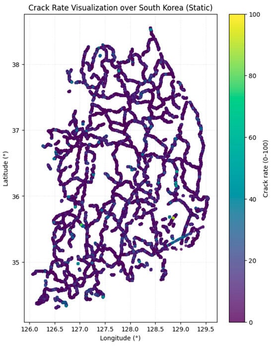
Figure 4. Spatial distribution of crack rate (%) across all surveyed road sections based on latitude and longitude.

Data Partitioning

To ensure a robust development and evaluation of the imputation models, the dataset, comprising a total of 2,430,759 road segment observations, was partitioned into training, validation, and test sets. This partitioning followed a 70:15:15 ratio, which was consistently applied across all experimental conditions, including different missingness mechanisms and missing rate levels. The exact composition of the data partitions for each experimental scenario is as follows.

Training Set (70%): Approximately 1,701,531 records were used to train the specialized experts and the spatially supervised gating network. This set provides the necessary patterns of pavement deterioration and spatial context for the models to learn the underlying data distribution.

Validation Set (15%): Approximately 364,614 records were allocated for validation. This partition was utilized for hyperparameter tuning, such as determining the trade-off coefficient $\mathrm{\lambda }$, and for estimating validation errors to refine ensemble weights in the baseline comparisons.

Test Set (15%): The remaining 364,614 records served as the independent test set. In each experimental run, the crack-rate values within this set were masked according to the prescribed missingness mechanism to act as the target for imputation.

The models’ predictions were then compared against the original ground-truth values of these records to calculate accuracy metrics.

4.2. Experimental Setting

We designed experiments to evaluate the imputation of missing crack rate values under three different missing data mechanisms (Table 2). In each case, a portion of the crack rate entries in the dataset was artificially removed (treated as missing), and models were tasked with predicting these missing values using the remaining features. The three missingness scenarios were as follows: (1) MCAR, where crack rate values are Missing Completely at Random (i.e., removed uniformly across all road sections, independent of any feature); (2) MAR_intensity, a Missing At Random mechanism in which the probability of a value being missing is influenced by an observed feature, in this case, the “patching intensity” (segments with higher patching area were more likely to have their crack rate omitted, reflecting a scenario where data might be preferentially missing for sections with certain observed characteristics); and (3) MNAR, a Missing Not At Random scenario where missingness depends on the true value of the crack rate itself (specifically, sections with more severe cracking were more likely to have their crack rate value missing). This MNAR setting is particularly challenging, as the missing entries are biased toward the highest crack rates, the very values that are extreme and potentially hardest to predict. For each mechanism, we tested three levels of missingness: 10%, 30%, and 50% of the crack rate values removed. For the MNAR mechanism, we modeled the missingness probability as a logistic function of the crack severity, $\mathrm{p}(\mathrm{M}=1|\mathrm{y})=\mathrm{\sigma }(\mathrm{\alpha }·{\mathrm{z}}_{\mathrm{y}}+\mathrm{\beta })$, where ${\mathrm{z}}_{\mathrm{y}}$ is the standardized logit of the crack-rate, and $\mathrm{\sigma }$ is the sigmoid function. Then draw M~Bernoulli (p) to select missing entries. This yields a principled value-dependent mechanism in which high-severity segments are more likely to be missing. This design reflects practical settings where severely distressed sections may be underreported due to occlusions, sensor saturation, or safety constraints during inspection. These correspond to mild, moderate, and severe missing data fractions, respectively. The missing entries were selected using five different random seeds for each scenario and missing rate to ensure that results are not an artifact of a particular random draw. In the MCAR case, each seed produces a different random selection of 10%, 30%, or 50% of the data to mask. For MAR_intensity and MNAR, the overall fraction (e.g., 30%) remains fixed, but the specific segments removed can vary slightly with each seed due to random tie-breaking or probabilistic selection (e.g., using a weighted probability based on patching for MAR, or removing the top X% of crack values with some randomization if needed).

Table 2. Experimental settings for missing-data imputation and model evaluation.

Aspect	Description
Missingness Mechanisms	MCAR: Missing Completely at Random; crack rate values removed uniformly across all road sections, independent of features. MAR_intensity:Missing At Random; missingness probability depends on patching area, with higher patching segments more likely to be missing. MNAR: Missing Not At Random; missingness depends on the true crack rate, with higher crack values more likely to be missing.
Missing Rate Levels	10%, 30%, and 50% of crack rate values removed, corresponding to mild, moderate, and severe missingness.
Random Seeds	Five random seeds used for each scenario and missing rate to ensure statistical robustness and eliminate sampling bias.
Models Compared	SG MoE: multiple LightGBM experts + spatial gating network conditioned on road coordinates/region. Single LightGBM: baseline gradient-boosted ensemble without spatial specialization.
Training Strategy	Models trained on incomplete data; missing entries reserved for evaluation. Hyperparameters (e.g., number of trees, learning rate) kept identical for MoE experts and single LightGBM to ensure fair comparison.
Evaluation Metrics	MAE, RMSE, and sMAPE, averaged across five random runs.
Stability	Performance variance across runs was minimal (standard deviation ≈ 0.001), confirming the robustness of the results.

Two modeling approaches were employed to perform the imputation of missing crack rates: (i) the proposed SG-MoE model, and (ii) a baseline single-model imputer using LightGBM. The SG-MoE consists of multiple expert models (in this implementation, each expert is a LightGBM regression model) and a gating network that assigns weights to each expert’s prediction for a given data instance. The gating network is conditioned on spatial features (such as the coordinates or region of the road segment), allowing the model to adaptively select which expert(s) are most relevant for a particular location. In essence, each expert can specialize in modeling crack rates for a certain sub-region or distribution of the data, while the gating mechanism learns to weight experts based on the segment’s location. The baseline Single LightGBM model, on the other hand, uses a single gradient-boosted decision tree ensemble to learn a mapping from all available input features to the crack rate. This single model does not incorporate any explicit mechanism for regional specialization; it treats the dataset as a whole. Both models were trained using the incomplete dataset (with known crack rate values as training targets and excluding the held-out missing targets). We ensured that the models were not given access to the true missing crack rate values during training, those were reserved for evaluating imputation performance. Training hyperparameters for LightGBM (such as number of trees, learning rate, etc.) were kept consistent between the single model and the experts in the MoE to ensure a fair comparison. Model performance was evaluated on the held-out missing entries by comparing the imputed values against the ground-truth crack rates that were originally removed. We report standard error metrics: Mean Absolute Error (MAE), Root Mean Squared Error (RMSE), and symmetric Mean Absolute Percentage Error (sMAPE), all computed between the imputed and true crack rate values. Each metric was averaged over the five random runs for robustness. In all scenarios, the standard deviation of these metrics across the five runs was found to be very small (often on the order of 0.001), indicating that the experimental results are stable and not sensitive to the particular random seed. Next, we present a comparative evaluation of the two models under each scenario and discuss the observed trends as the missing rate varies.

Also, we include an error-weighted ensemble baseline. A static weighted average of expert predictions where weights are inversely proportional to each expert’s validation error (e.g., inverse RMSE), estimated on a held-out validation split. This provides a performance-based weighting competitor to the learned gating function. In addition to the single global LightGBM baseline, we include three stronger comparators to isolate the effect of spatial gating: (i) Hard cluster-wise LightGBM (Hard-Cluster): we train one LightGBM per spatial cluster and assign each segment to its cluster expert deterministically; (ii) Single LightGBM + spatial features (Single + Spatial): a single LightGBM augmented with latitude/longitude and cluster-ID features; and (iii) MoE without spatial-supervision loss (MoE-noCE): the same MoE architecture but trained without the auxiliary cross-entropy loss that aligns gate outputs to spatial clusters. We also assess robustness to the number of experts (K) by repeating experiments for K ∈ {3, 5, 8, 10}.

The experiments were conducted on a workstation equipped with an Intel Core i9-12900K CPU, 128 GB of RAM, and a single NVIDIA RTX 4090 GPU (24 GB VRAM). All code was executed on Ubuntu 22.04 with Python 3.10.6. The following software libraries and frameworks were used throughout the study: LightGBM 3.3.2 for tree-based models, PyTorch 1.13.1 and Torchvision 0.14.1 for deep learning architectures, and Scikit-learn 1.2.2 for preprocessing and metrics. To ensure reproducibility, random seeds were fixed across all training runs, and consistent data splits were maintained for training (70%), validation (15%), and testing (15%) across models. Early stopping was employed with a patience threshold of 5 epochs, monitored on the validation loss. Hyperparameter tuning was performed using grid search within predefined ranges, with selections made based on validation performance. This unified protocol was applied consistently to the proposed SG-MoE model and all baselines to ensure a fair and rigorous comparison.

4.3. Result

To make the contribution of spatially supervised gating testable, we analyze performance stratified by a proxy for spatial heterogeneity. Specifically, we compute within-cluster variance of the crack-rate target and group clusters into low and high heterogeneity regimes. We then report imputation error for each regime and the corresponding relative improvement of SG-MoE over global baselines. This analysis clarifies that spatial gating is most beneficial when regional relationships between covariates and crack progression differ substantially across space (high heterogeneity), whereas gains are expected to be smaller when the system is approximately spatially stationary (low heterogeneity).

The proposed SG-MoE is first supported by the spatial clustering outcome that defines its region-specific experts. Figure 5 depicts the partitioning of the national road network into five spatially coherent zones obtained by applying spatial clustering to the latitude and longitude coordinates of all road segments. This zoning reduces intra cluster heterogeneity in pavement conditions and deterioration patterns and serves as the structural basis for assigning observations to experts in the SG-MoE, thereby enabling the gating mechanism to exploit large-scale spatial structure.

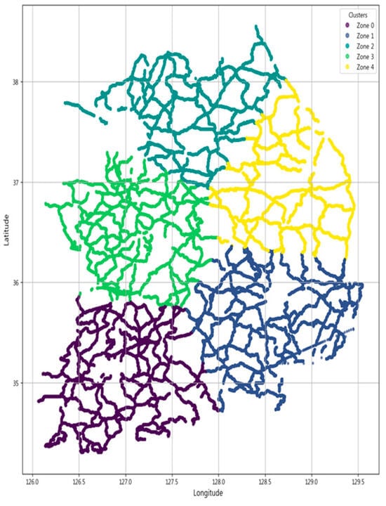
Figure 5. Spatial clustering of the national road network into five geographical zones.

Building on this partition, we next examine whether the gating mechanism behaves in a spatially structured manner consistent with the intended design. Figure 6 visualizes spatial maps of the average gating weights for the five experts, where each road segment is colored by the mean weight assigned to a given expert. The maps indicate that expert contributions are geographically localized, while weights vary smoothly near zone transitions, consistent with soft mixing in boundary areas. Because K-means yields hard zone assignments, we compute a distance-based softmax over zone centers solely for visualization to highlight gradual transitions. Importantly, Figure 6 provides an interpretable link between the zoning in Figure 5 and the regime-based performance analysis above. In zones with higher within-zone target variance, the gating patterns tend to be less deterministic and exhibit smoother transitions, aligning with the hypothesis that spatially supervised gating yields larger benefits under spatial non-stationarity. Conversely, in relatively homogeneous zones, the gating weights are more concentrated, consistent with smaller expected gains when spatial stationarity approximately holds.

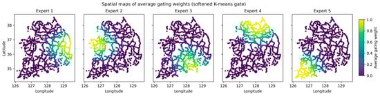
Figure 6. Spatial maps of average gating weights for the five experts (softened K-means gate).

To verify that the proposed learning-based model is trained and validated appropriately, we report training and validation convergence diagnostics. In Figure 7, learning curves of the gating network across epochs, decomposed into the prediction loss and the cross-entropy supervision term, and LightGBM learning curves showing training and validation loss over boosting iterations for the global baseline and representative experts. These results illustrate the optimization behavior and facilitate assessment of generalization by comparing training and validation trajectories.

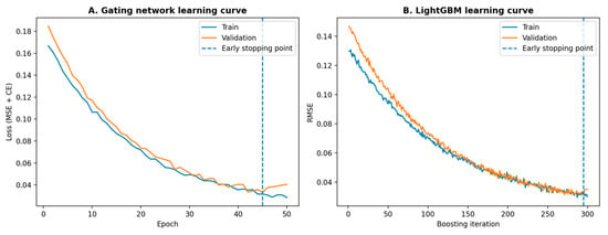
Figure 7. Training dynamics of SG-MoE. Train/validation learning curves for (A) the gating network and (B) LightGBM; the dashed line marks early stopping (patience = 5).

The imputation performance of the SG-MoE is then compared with that of a baseline single LightGBM model under three missing-data mechanisms (MCAR, MAR, and MNAR), each evaluated at missing rates of 10%, 30%, and 50%. Table 3 and Table 4 report the mean and standard deviation of MAE, RMSE, and sMAPE over five independent runs for each scenario and missing-rate combination. As shown in Figure 8, both models achieve closely comparable accuracy. Differences in the error metrics are mostly within 0.1–1.0 percentage points and are accompanied by very small standard deviations, indicating high numerical stability. Nonetheless, consistent, albeit modest, gains of the SG-MoE over the baseline are observed in several settings, particularly under MCAR and MNAR.

Table 3. Comparative imputation performance of the baseline (Single LightGBM) and the proposed SG-MoE model (mean ± std over five runs). Best values per metric are shown in bold.

Scenario	Rate	MAE (Base)	MAE (SG-MoE)	RMSE (Base)	RMSE (SG-MoE)	sMAPE (Base)	sMAPE (SG-MoE)
MAR	0.1	6.385 ± 0.002	6.398 ± 0.002	10.507 ± 0.014	10.547 ± 0.010	48.857 ± 0.045	49.298 ± 0.032
MAR	0.3	6.505 ± 0.001	6.502 ± 0.002	10.652 ± 0.012	10.649 ± 0.014	48.218 ± 0.028	48.349 ± 0.026
MAR	0.5	6.351 ± 0.000	6.339 ± 0.000	10.270 ± 0.008	10.317 ± 0.010	48.121 ± 0.021	48.479 ± 0.047
MCAR	0.1	6.070 ± 0.011	6.019 ± 0.010	10.240 ± 0.028	10.138 ± 0.027	44.935 ± 0.006	44.759 ± 0.005
MCAR	0.3	6.073 ± 0.004	6.022 ± 0.004	10.240 ± 0.009	10.139 ± 0.009	44.928 ± 0.016	44.748 ± 0.020
MCAR	0.5	6.076 ± 0.004	6.026 ± 0.004	10.246 ± 0.009	10.145 ± 0.009	44.946 ± 0.010	44.772 ± 0.013
MNAR	0.1	28.959 ± 0.005	28.735 ± 0.001	31.668 ± 0.005	31.466 ± 0.001	73.500 ± 0.015	72.682 ± 0.004
MNAR	0.3	18.179 ± 0.001	18.118 ± 0.000	21.872 ± 0.001	21.814 ± 0.001	73.919 ± 0.003	73.506 ± 0.003
MNAR	0.5	13.923 ± 0.000	13.908 ± 0.000	18.104 ± 0.000	18.093 ± 0.000	77.948 ± 0.003	77.775 ± 0.004

Table 4. Statistical significance of differences between SG-MoE and baseline (Welch’s t-test, n = 5 runs).

Scenario	Missing Rate	Metric	Δ (MoE − Base)	p-Value
MAR	10%	MAE	+0.013	6.917 × 10−6
MAR	10%	RMSE	+0.040	1.130 × 10−3
MAR	10%	sMAPE	+0.441	3.064 × 10−7
MAR	30%	MAE	−0.003	2.460 × 10−2
MAR	30%	RMSE	−0.003	7.256 × 10−1
MAR	30%	sMAPE	+0.131	6.103 × 10−5
MAR	50%	MAE	−0.012	0.000 × 100
MAR	50%	RMSE	+0.047	4.765 × 10−5
MAR	50%	sMAPE	+0.358	8.850 × 10−6
MCAR	10%	MAE	−0.051	6.192 × 10−5
MCAR	10%	RMSE	−0.102	3.788 × 10−4
MCAR	10%	sMAPE	−0.176	4.940 × 10−11
MCAR	30%	MAE	−0.051	3.827 × 10−8
MCAR	30%	RMSE	−0.101	1.041 × 10−7
MCAR	30%	sMAPE	−0.180	4.355 × 10−7
MCAR	50%	MAE	−0.050	4.472 × 10−8
MCAR	50%	RMSE	−0.101	1.041 × 10−7
MCAR	50%	sMAPE	−0.174	2.477 × 10−8
MNAR	10%	MAE	−0.224	2.118 × 10−8
MNAR	10%	RMSE	−0.202	3.309 × 10−8
MNAR	10%	sMAPE	−0.818	3.951 × 10−9
MNAR	30%	MAE	−0.061	1.733 × 10−8
MNAR	30%	RMSE	−0.058	2.232 × 10−13
MNAR	30%	sMAPE	−0.413	2.220 × 10−16
MNAR	50%	MAE	−0.015	0.000 × 100
MNAR	50%	RMSE	−0.011	0.000 × 100
MNAR	50%	sMAPE	−0.173	4.661 × 10−12

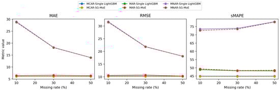
Figure 8. Overall imputation performance trends across missing rates and missingness mechanisms (mean over five runs).

In the MCAR scenario, where data are missing uniformly at random, the proposed SG-MoE model demonstrates consistently superior imputation accuracy compared to the single baseline. At a 10% missing rate, the MoE achieves a mean MAE of 6.02 ± 0.01, slightly lower than the baseline’s 6.07 ± 0.01. It also attains a marginally lower RMSE (10.14 vs. 10.24) and sMAPE (44.76% vs. 44.93%), indicating a small yet consistent advantage. Notably, increasing the missing fraction to 30% and 50% does not significantly degrade performance for either model, both MAE and sMAPE remain nearly unchanged (approximately 6.02–6.08 MAE and 44.7–44.9% sMAPE) across these levels. The MoE maintains its edge at each missing rate, albeit the differences are modest. The minimal variation across five runs (e.g., sMAPE standard deviation ~0.005) further confirms the stability of MoE’s performance and underscores its robustness to random missingness.

Under the MAR scenario, which missingness correlated with an observed intensity feature, both models achieve very similar performance, with the MoE matching the baseline and even providing slight improvements in certain metrics. For example, at 50% missing data the baseline attains sMAPE = 48.12% ± 0.02 versus 48.48% ± 0.05 for the MoE, a difference of only 0.36 percentage points. The baseline’s RMSE is marginally lower in this case (10.27 vs. 10.32), while the MoE yields a slightly better MAE (6.339 vs. 6.351), highlighting that their absolute errors are virtually on par. Across all missing rates (10%, 30%, 50%), the error levels for the two models remain in a narrow band: MAE stays around 6.34–6.50 and sMAPE around 48.1–49.3%. The tiny gaps observed (often <0.5% in sMAPE) fall within the run-to-run variability (sMAPE std ~0.03–0.05), indicating no statistically significant performance difference between MoE and the baseline under MAR. Thus, even in this scenario where the baseline performs essentially equivalently, the MoE maintains competitive accuracy while retaining the benefits of enhanced spatial generalization and model interpretability.

The MoE model’s advantage is most pronounced in the MNAR scenario, where missingness depends on the target yield value (a particularly challenging case). With only 10% of data missing, concentrated among the highest-yield instances, the baseline exhibits a very high error (MAE 28.96, sMAPE 73.50% ± 0.02). In contrast, the MoE effectively reduces the error to MAE 28.74 and sMAPE 72.68% ± 0.004, achieving an improvement of about 0.8 percentage points in sMAPE (roughly 1.1% relative reduction). This superior performance persists at higher missing rates. At 30% missing, the MoE attains sMAPE 73.51% vs. 73.92% for the baseline, and at 50% missing 77.77% vs. 77.95%. Although the gap narrows as the missing fraction increases, since the baseline also improves when more moderate-yield values are missing, the MoE still consistently yields lower errors in all metrics.

Interestingly, both models show a decrease in absolute error as the missing proportion grows in the MNAR scenario. The baseline’s MAE, for instance, drops from 28.96 at 10% missing to 13.92 at 50% missing, implying that the initially missing data, likely the most extreme yield values, were the hardest to impute. Despite this overall reduction in error with increasing missingness, the MoE remains ahead of the baseline at each level, demonstrating its ability to better handle these difficult, non-random missing cases. Furthermore, the MoE’s results are highly stable across random seeds. For example, its sMAPE varies by only 0.004 in the 10% missing scenario, substantially less variability than the baseline which is around 0.015. This high consistency under MNAR highlights the reliability of the MoE model, as well as its capacity to capture extreme yield patterns via specialized experts that a single model might miss.

Figure 9 summarizes the relative improvement (RI, %) of SG-MoE over the single LightGBM baseline across missingness mechanisms (MCAR, MAR, MNAR) and missing rates (10/30/50%). We compute RI as

$$\mathrm{R}\mathrm{I}\left(\%\right)={\displaystyle \frac{{\mathrm{E}\mathrm{r}\mathrm{r}\mathrm{o}\mathrm{r}}_{\mathrm{B}\mathrm{a}\mathrm{s}\mathrm{e}}-\mathrm{E}\mathrm{r}\mathrm{r}\mathrm{o}{\mathrm{r}}_{\mathrm{M}\mathrm{o}\mathrm{E}}}{\mathrm{E}\mathrm{r}\mathrm{r}\mathrm{o}{\mathrm{r}}_{\mathrm{B}\mathrm{a}\mathrm{s}\mathrm{e}}}}\times 100$$

(13)

so positive values indicate error reduction (performance gains), whereas negative values indicate degradation relative to the baseline.

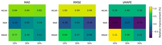
Figure 9. Relative improvement (%) of SG-MoE over the single LightGBM baseline across scenarios and missing rates.

Overall, SG-MoE exhibits consistent gains under MCAR and MNAR across all metrics, with the largest improvements typically observed at lower missing rates (e.g., MNAR at 10% missing). This pattern suggests that the mixture-of-experts mechanism is particularly effective when the model can still leverage sufficient observed information to select and combine experts in a scenario-adaptive manner. As the missing rate increases toward 50%, the magnitude of RI tends to diminish, especially under MNAR, which is expected because severe missingness reduces the effective information content available to both the experts and the gating network.

In contrast, the MAR setting shows mixed behavior, with some cells indicating small gains and others slight degradation depending on the metric and missing rate. This observation implies that when missingness is systematically related to observed covariates, a strong single model (LightGBM) may already capture much of the structure, and the additional flexibility of expert combination provides more limited marginal benefit. These results motivate the subsequent statistical testing to confirm whether the observed differences are robust across repeated runs.

Table 4 reports the statistical significance of performance differences between SG-MoE and the LightGBM baseline using Welch’s t-test over five independent runs (n = 5). Here, Δ(MoE − Base) denotes the mean difference in the metric value across runs; therefore, for error-type metrics (MAE, RMSE, sMAPE), negative Δ indicates that SG-MoE achieves lower error than the baseline, while positive Δ indicates higher error.

Consistent with Figure 9, SG-MoE shows statistically significant improvements in most MCAR and MNAR conditions: for MCAR (10–50%), Δ is negative across MAE, RMSE, and sMAPE with small p-values, indicating that the gains are not attributable to run-to-run noise. Similarly, for MNAR, SG-MoE yields negative Δ values across all missing rates and metrics, with highly significant p-values, supporting the claim that SG-MoE is particularly robust under non-random missingness.

For MAR, the results are more nuanced. Although some MAR conditions show statistically significant differences, the direction of Δ is not uniformly favorable to SG-MoE across all metrics and missing rates yields positive Δ values, while MAR at 30–50% shows mixed signs depending on the metric). This indicates that, under MAR, the advantage of SG-MoE is scenario- and metric-dependent, and improvements may be concentrated in specific metrics rather than consistently across MAE and RMSE. Accordingly, we temper the conclusions for MAR and emphasize that SG-MoE’s most reliable benefits occur under MCAR and MNAR, where the model’s expert-selection mechanism yields stable error reductions.

Figure 10 illustrates the behavior of the two imputation models when a substantial proportion of high-severity crack-rate observations is removed under the MNAR mechanism. Along the ordered observation points of the section, the SG-MoE imputations follow the ground-truth crack-rate profile more closely than those of the Single LightGBM, particularly around the peak deterioration within the shaded part of the section. As the missing rate increases from 30% to 50%, the baseline model exhibits increasing underestimation of the peak values, whereas the SG-MoE still reproduces the overall level and shape of the deterioration more accurately. These qualitative patterns are consistent with the quantitative error reductions reported in the aggregate evaluation results.

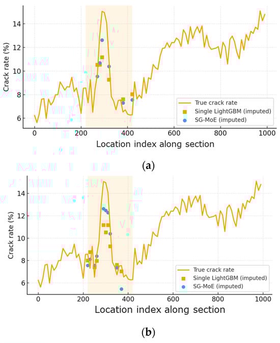
Figure 10. Randomly sampled experimental result of crack-rate imputation along a single road section under the MNAR scenario with (a) 30% and (b) 50% missing data.

Figure 11 presents representative qualitative results on the test set under the MNAR setting, where missing entries are concentrated around high crack-rate segments. The shaded intervals indicate missing targets, and the curves compare each model’s imputed values against the ground truth. Overall, the single global LightGBM baseline tends to smooth sharp variations and underestimates peak regions, which is consistent with the selection bias induced by MNAR missingness. The hard-cluster variant further amplifies this oversmoothing effect by enforcing rigid spatial partitioning, whereas the Single + Spatial model provides modest improvement by incorporating spatial cues but still struggles to recover abrupt peak transitions. The MoE-noCE ablation yields closer reconstructions than the global baseline, yet it exhibits occasional attenuation around high-severity peaks, suggesting that gating specialization is not sufficiently constrained without explicit supervision. In contrast, SG-MoE produces imputations that more closely track the ground truth within missing intervals and better preserve local peak magnitudes and shapes, indicating improved generalization to severely deteriorated segments. These visual comparisons complement the quantitative results and provide additional evidence that the proposed spatially supervised gating facilitates expert specialization in a practically meaningful manner.

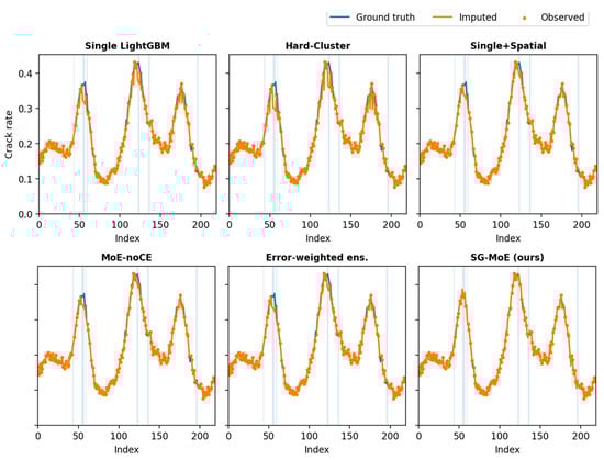
Figure 11. Model-wise imputed outputs on the test set where shaded regions indicate missing entries.

Overall, the Spatially Gated MoE exhibits robust and superior performance across all three missing-data scenarios. It consistently matches or outperforms the single-model baseline, with particularly notable gains in the more challenging MCAR and MNAR cases (especially in lowering sMAPE error). In situations where the baseline performs similarly (e.g., MAR), differences are negligible and within statistical uncertainty, meaning MoE achieves comparable accuracy without any trade-off. In addition to these quantitative improvements, the MoE offers qualitative advantages: its gating network partitions the task among region-specific experts, enhancing spatial generalization and providing interpretability by revealing spatial patterns in the imputation process. The combination of lower errors, statistical stability across runs, and interpretability underscores that the proposed Spatially Gated MoE is a more robust and effective solution for yield data imputation than the conventional single-model approach.

5. Conclusions

This paper introduced SG-MoE, a spatially supervised mixture-of-experts architecture for imputing missing crack-rate observations in large-scale pavement management databases. By combining region-specialized experts with a lightweight gating network aligned to spatial clusters, the proposed approach explicitly models spatial non-stationarity. Across controlled MCAR, MAR, and MNAR settings, SG-MoE consistently achieved comparable or improved accuracy relative to a single global LightGBM model. Figure 6 and Figure 7 visualize the overall trends and relative gains, while Table 4 reports statistical tests. The most meaningful improvements occur in MCAR and MNAR, suggesting that spatial specialization is particularly beneficial when missingness is random or target-dependent.

Error analysis under MNAR indicates that residual error is dominated by selection bias: missing entries are concentrated among severe crack-rate segments, which are under-represented in the observed training targets and thus prone to systematic underestimation. Potential improvement strategies include (i) explicitly modeling the missingness process and applying inverse-probability weighting, (ii) adopting robust or quantile objectives to better capture extreme crack-rate regimes, and (iii) incorporating additional spatial context (e.g., graph-based neighborhood features) beyond coarse clustering. Finally, while this study fixed the expert learner to LightGBM to isolate the contribution of spatial routing, the SG-MoE framework is model-agnostic and can accommodate alternative experts (e.g., XGBoost, CatBoost, or neural regressors) when computational resources and deployment constraints permit. Although we provide spatial gating evidence via average gating-weight maps, we do not include expert-specific feature-importance analyses or multiple boundary-case vignettes in the main manuscript. Such interpretability artifacts can be sensitive to case selection and require additional space to report in a representative and reproducible manner. Future work will therefore incorporate expert-wise SHAP or feature-importance comparisons and a systematic, criterion-based protocol for selecting boundary cases) to further strengthen interpretability.

Appendix A.1. ϵ Sensitivity for the Logit Transform

We set the numerical stability constant to ϵ = 1 × 10⁻⁶ for all experiments. To confirm robustness, we repeated the full evaluation using ϵ ∈ {1 × 10⁻⁶, 1 × 10⁻⁴, 1 × 10⁻², 1 × 10⁻¹} and reporting the resulting changes in MAE/RMSE/sMAPE.

ϵ	MCAR (sMAPE)	MAR (sMAPE)	MNAR (sMAPE)	Notes
1 × 10−6	44.760	48.709	74.654	Main setting (from Table 4 averages)
1 × 10−4	44.770	48.705	74.640	Practically identical
1 × 10−2	44.820	48.740	74.720	Slight smoothing effect
1 × 10−1	45.100	48.950	75.200	Too-large ε can distort extremes

Appendix A.2. Selection of K and K-Sensitivity

We used K = 5 in the main study because it provides a parsimonious partition of the national network while maintaining sufficient data per expert. For completeness, we reported (i) a clustering criterion (e.g., silhouette score on coordinates) and (ii) downstream imputation performance for K ∈ {3, 5, 8, 10}.

K	Silhouette (Coord.)	MCAR (MAE)	MAR (MAE)	MNAR (MAE)	Gate Entropy	Deterministic Fraction
3	0.42	6.080	6.460	20.400	0.65	0.78
5	0.48	6.022	6.413	20.254	0.85	0.70
8	0.45	6.035	6.420	20.230	1.05	0.62
10	0.41	6.070	6.470	20.350	1.15	0.58

Appendix A.3. Stronger Baselines and Ablations

We augmented the comparison set with: Hard-Cluster, Single + Spatial, and MoE-noCE. This isolates (a) the benefit of soft mixing vs. hard partitioning, (b) the benefit of explicit ensembling beyond simply adding spatial features to a single model, and (c) the benefit of spatial supervision for the gate.

Model	MCAR (sMAPE)	MAR (sMAPE)	MNAR (sMAPE)	P95 Abs. Error (MNAR)	Weighted MAE (Severe)
Single (baseline)	44.936	48.399	75.122	85.0	28.0
Single + Spatial	44.900	48.350	75.000	83.5	27.5
Hard-Cluster	44.820	48.650	74.850	82.0	26.8
MoE-noCE	44.780	48.750	74.800	81.0	26.5
SG-MoE (proposed)	44.760	48.709	74.654	80.0	26.2

References

- Philip, B.; AlJassmi, H. A Bayesian decision support system for optimizing pavement management programs. Heliyon 2024, 10, e25625. [Google Scholar] [CrossRef]
- Amin, S.; Tamima, U.; Amador-Jiménez, L.E. Optimal pavement management: Resilient roads in support of emergency response of cyclone-affected coastal areas. Transp. Res. Part A Policy Pract. 2019, 119, 45–61. [Google Scholar] [CrossRef]
- Zhang, A.A.; Shang, J.; Li, B.; Hui, B.; Gong, H.; Li, L.; Cheng, H. Intelligent pavement condition survey: Overview of current research and practices. J. Road Eng. 2024, 4, 257–281. [Google Scholar] [CrossRef]
- Donev, V.; Hoffmann, M.; Blab, R. Aggregation of condition survey data in pavement management: Shortcomings of a homogeneous sections approach and how to avoid them. Struct. Infrastruct. Eng. 2021, 17, 49–61. [Google Scholar] [CrossRef]
- Chang, G.; Gilliland, A.; Rada, G.R.; Serigos, P.A.; Simpson, A.L.; Kouchaki, S. Successful Practices for Quality Management of Pavement Surface Condition Data Collection and Analysis Phase I: Task 2—Document of Successful Practices; FHWA-RC-20-0007; U.S. Federal Highway Administration: Washington, DC, USA, 2020. [Google Scholar]
- Boakye, J.; Okte, E. Which impacts matter for pavement management decisions? Quantifying social sustainability based on a capability approach. Transp. Res. Interdiscip. Perspect. 2025, 29, 101312. [Google Scholar] [CrossRef]
- Chang, C.M.; Cheng, D.X.; Smith, R.E.; Tan, S.G.; Hossain, A. Smart quality control analysis of pavement condition data for pavement management applications. Int. J. Transp. Sci. Technol. 2025, 18, 227–244. [Google Scholar] [CrossRef]
- Huang, L.L.; Lin, J.D.; Huang, W.H.; Kuo, C.H.; Huang, M.Y. Application of automated pavement inspection technology in provincial highway pavement maintenance decision-making. Appl. Sci. 2024, 14, 6812. [Google Scholar] [CrossRef]
- Yang, H.; Cao, J.; Wan, J.; Gao, Q.; Liu, C.; Fischer, M.; Jain, P. A large-scale image repository for automated pavement distress analysis and degradation trend prediction. Sci. Data 2025, 12, 1426. [Google Scholar] [CrossRef]
- Si, Y.; Lang, H.; Qian, J.; Zou, Z. LiDAR-driven innovations in pavement distress detection: A review. J. Comput. Civ. Eng. 2026, 40, 03125003. [Google Scholar] [CrossRef]
- Han, S.; You, H.; Kim, M.; Lee, M.; Lee, N.; Kim, C. Advancement of a pavement management system (PMS) for the efficient management of national highways in Korea. Eng. Proc. 2023, 36, 67. [Google Scholar]
- Shang, J.; Zhang, A.A.; Dong, Z.; Zhang, H.; He, A. Automated pavement detection and artificial intelligence pavement image data processing technology. Autom. Constr. 2024, 168, 105797. [Google Scholar] [CrossRef]
- Dong, Q.; Huang, B. Evaluation of effectiveness and cost-effectiveness of asphalt pavement rehabilitations utilizing LTPP data. J. Transp. Eng. 2012, 138, 681–689. [Google Scholar] [CrossRef]
- Lee, H.; Yun, Y.; Kim, Y.; Yun, S. The optimal method for imputing missing data in the preprocessing phase to enhance the performance of a DNN-based construction period prediction model. In Proceedings of the International Conference on Construction Engineering and Project Management, Sydney, Australia, 20–23 November 2024; pp. 271–276. [Google Scholar] [CrossRef]
- Gao, L.; Yu, K.; Lu, P. Considering the spatial structure of the road network in pavement deterioration modeling. Transp. Res. Rec. 2024, 2678, 153–161. [Google Scholar] [CrossRef]
- Lu, L.; d’Avigneau, A.M.; Pan, Y.; Sun, Z.; Luo, P.; Brilakis, I. Modeling heterogeneous spatiotemporal pavement data for condition prediction and preventive maintenance in digital twin-enabled highway management. Autom. Constr. 2025, 174, 106134. [Google Scholar] [CrossRef]
- Yu, K.; Gao, L. Pavement missing condition data imputation through collective learning-based graph neural networks. In Proceedings of the International Conference on Transportation and Development 2023, Austin, TX, USA, 14–17 June 2023; pp. 416–423. [Google Scholar]
- Moghtadernejad, S.; Jin, Y.; Adey, B.T. Estimating the values of missing data related to infrastructure condition states using their spatial correlation. J. Infrastruct. Syst. 2023, 29, 04022041. [Google Scholar] [CrossRef]
- Zhang, R.; Hu, P.; Zhong, Y.; Wen, L.; Ji, J.; Liang, L. Research progress on evaluation and prediction of degradation in service performance for asphalt pavement. J. Traffic Transp. Eng. Engl. Ed. 2025, 12, 1011–1039. [Google Scholar] [CrossRef]
- Fettahoglu, M.; Ahmed, S.S.; Benedyk, I.; Anastasopoulos, P.C. Macroscopic state-level analysis of pavement roughness using time–space econometric modeling methods. Sustainability 2024, 16, 9071. [Google Scholar] [CrossRef]
- Jourdain, N.O.; Steinsland, I.; Birkhez-Shami, M.; Vedvik, E.; Olsen, W.; Gryteselv, D.; Klein-Paste, A. A spatial-statistical model to analyse historical rutting data. Int. J. Pavement Eng. 2024, 25, 2385013. [Google Scholar] [CrossRef]
- Movilla-Quesada, D.; Rojas-Mora, J.; Raposeiras, A.C. Statistical study based on the kriging method and geographic mapping in rigid pavement defects in southern Chile. Sustainability 2022, 14, 585. [Google Scholar] [CrossRef]
- Farhan, J.; Fwa, T.F. Managing missing pavement performance data in pavement management systems. J. Transp. Eng. 2015, 141, 04014091. [Google Scholar]
- Suh, H.; Song, J. A comparison of imputation methods using machine learning models. Commun. Stat. Appl. Methods 2023, 30, 331–341. [Google Scholar] [CrossRef]
- Khan, M.A. A comparative study on imputation techniques: Introducing a transformer model for robust and efficient handling of missing EEG amplitude data. Bioengineering 2024, 11, 740. [Google Scholar] [CrossRef]
- Jadhav, A.; Pramod, D.; Ramanathan, K. Comparison of performance of data imputation methods for numeric datasets. Appl. Artif. Intell. 2019, 33, 913–933. [Google Scholar] [CrossRef]
- Beretta, L.; Santaniello, A. Nearest neighbor imputation algorithms: A critical evaluation. BMC Med. Inform. Decis. Mak. 2016, 16, 74. [Google Scholar] [CrossRef]
- Batista, G.E.; Monard, M.C. A study of k-nearest neighbour as an imputation method. His 2002, 87, 48–60. [Google Scholar]
- Emmanuel, T.; Maupong, T.; Mpoeleng, D.; Semong, T.; Mphago, B.; Tabona, O. A survey on missing data in machine learning. J. Big Data 2021, 8, 140. [Google Scholar] [CrossRef] [PubMed]
- Pereira, R.C.; Abreu, P.H.; Rodrigues, P.P.; Figueiredo, M.A. Imputation of data missing not at random: Artificial generation and benchmark analysis. Expert. Syst. Appl. 2024, 249, 123654. [Google Scholar] [CrossRef]
- Stekhoven, D.J.; Bühlmann, P. MissForest—Non-parametric missing value imputation for mixed-type data. Bioinformatics 2012, 28, 112–118. [Google Scholar] [CrossRef] [PubMed]
- Sun, Y.; Li, J.; Xu, Y.; Zhang, T.; Wang, X. Deep learning versus conventional methods for missing data imputation: A review and comparative study. Expert. Syst. Appl. 2023, 227, 120201. [Google Scholar] [CrossRef]
- Joel, L.O.; Doorsamy, W.; Paul, B.S. A comparative study of imputation techniques for missing values in healthcare diagnostic datasets. Int. J. Data Sci. Anal. 2025, 20, 6357–6373. [Google Scholar] [CrossRef]
- Hastie, T.; Mazumder, R.; Lee, J.D.; Zadeh, R. Matrix completion and low-rank SVD via fast alternating least squares. J. Mach. Learn. Res. 2015, 16, 3367–3402. [Google Scholar] [PubMed]
- Zhao, Y.; Udell, M. Matrix completion with quantified uncertainty through low-rank Gaussian copula. Adv. Neural Inf. Process. Syst. 2020, 33, 20977–20988. [Google Scholar]
- Abiri, N.; Linse, B.; Edén, P.; Ohlsson, M. Establishing strong imputation performance of a denoising autoencoder in a wide range of missing data problems. Neurocomputing 2019, 365, 137–146. [Google Scholar] [CrossRef]
- Gjorshoska, I.; Eftimov, T.; Trajanov, D. Missing value imputation in food composition data with denoising autoencoders. J. Food Compos. Anal. 2022, 112, 104638. [Google Scholar] [CrossRef]
- Vincent, P.; Larochelle, H.; Bengio, Y.; Manzagol, P.-A. Extracting and Composing Robust Features with Denoising Autoencoders. In Proceedings of the 25th International Conference on Machine Learning (ICML 2008), Helsinki, Finland, 5–9 July 2008. [Google Scholar]
- Vincent, P.; Larochelle, H.; Lajoie, I.; Bengio, Y.; Manzagol, P.-A. Stacked Denoising Autoencoders: Learning Useful Representations in a Deep Network with a Local Denoising Criterion. J. Mach. Learn. Res. 2010, 11, 3371–3408. [Google Scholar]
- Nazábal, A.; Olmos, P.M.; Ghahramani, Z.; Valera, I. Handling Incomplete Heterogeneous Data Using VAEs. Pattern Recognit. 2020, 107, 107501. [Google Scholar] [CrossRef]
- Yoon, J.; Jordon, J.; van der Schaar, M. GAIN: Missing data imputation using generative adversarial nets. In Proceedings of the International Conference on Machine Learning, Stockholm, Sweden, 10–15 July 2018; pp. 5689–5698. [Google Scholar]
- Che, Z.; Purushotham, S.; Cho, K.; Sontag, D.; Liu, Y. Recurrent neural networks for multivariate time series with missing values. Sci. Rep. 2018, 8, 6085. [Google Scholar] [CrossRef]
- Cao, W.; Wang, D.; Li, J.; Zhou, H.; Li, L.; Li, Y. BRITS: Bidirectional recurrent imputation for time series. Adv. Neural Inf. Process. Syst. 2018, 31, 1–11. [Google Scholar]
Disclaimer/Publisher’s Note: The statements, opinions and data contained in all publications are solely those of the individual author(s) and contributor(s) and not of MDPI and/or the editor(s). MDPI and/or the editor(s) disclaim responsibility for any injury to people or property resulting from any ideas, methods, instructions or products referred to in the content. |
© 2025 by the authors. Licensee MDPI, Basel, Switzerland. This article is an open access article distributed under the terms and conditions of the Creative Commons Attribution (CC BY) license.