State-Space and Multi-Scale Convolutional Generative Adversarial Network for Traffic Flow Forecasting

Abstract

Long-sequence traffic flow forecasting plays a crucial role in intelligent transportation systems. However, existing Transformer-based approaches face a quadratic complexity bottleneck in computation and are prone to over-smoothing in deep architectures. This results in overly averaged predictions that fail to capture the peaks and troughs of traffic flow. To address these issues, we propose a State-Space Generative Adversarial Network (SSGAN) with a state-space generator and a multi-scale convolutional discriminator. Specifically, a bidirectional Mamba-2 model was designed as the generator to leverage the linear complexity and efficient forecasting capability of state-space models for long-sequence modeling. Meanwhile, the discriminator incorporates a multi-scale convolutional structure to extract traffic features from the frequency domain, thereby capturing flow patterns across different scales, alleviating the over-smoothing issue and enhancing discriminative ability. Through adversarial training, the model is able to better approximate the true distribution of traffic flow. Experiments conducted on four real-world public traffic flow datasets demonstrate that the proposed method outperformed the baselines in both forecasting accuracy and computational efficiency.

1. Introduction

With the acceleration of urbanization and the continuous growth of traffic demand, accurate and efficient traffic flow forecasting has become one of the core issues in intelligent transportation systems. High-precision traffic forecasting not only helps alleviate congestion and optimize travel routes but also provides crucial decision-making support for urban planning and traffic management [1,2,3,4,5]. However, traffic flow data typically exhibit strong temporal dependencies and non-stationarity, which makes modeling particularly challenging in long-term forecasting tasks.

Deep learning methods have achieved remarkable progress in traffic forecasting. Among them, Transformer-based approaches [6] have attracted widespread attention due to their strong capability in temporal modeling [7,8,9,10,11,12,13]. Nevertheless, in long-sequence forecasting scenarios, the quadratic complexity of the Transformer attention mechanism results in substantial computational overhead, limiting the efficiency of such models on large-scale datasets [14]. Recently, state-space models (SSMs) have emerged as a powerful alternative for long-sequence modeling. Unlike attention-based Transformers, SSMs model long-range dependencies through recursive hidden states and convolutional kernel expansion, achieving linear time complexity while effectively capturing long-term dependencies. In particular, a series of improved SSMs [15,16,17,18] have demonstrated superior performance and strong long-sequence modeling ability in time series forecasting tasks. This provides a new perspective for traffic flow forecasting, namely leveraging state-space models to enhance both predictive accuracy and computational efficiency.

In traffic flow forecasting tasks, traditional methods commonly adopt the Mean Squared Error (MSE) or Mean Absolute Error (MAE) as optimization objectives. However, such regression losses inherently encourage models to produce “averaged” predictions to minimize overall error, leading to pronounced over-smoothing at peaks and abrupt changes [19]. Consequently, the predicted sequences fail to capture fine-grained temporal dynamics and overlook the true peaks and troughs in traffic flow, thereby degrading forecasting accuracy, as illustrated in Figure 1. Over-smoothing not only weakens the model’s ability to detect sharp fluctuations in traffic flow, but also limits the practical applicability of forecasting results in real-world traffic management scenarios.

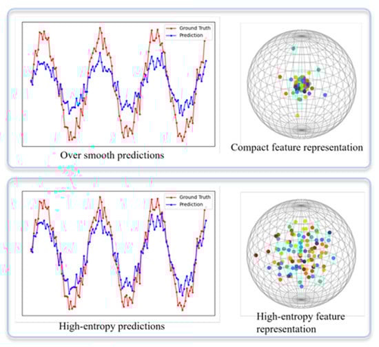
Figure 1. Over-smoothing problem.

To mitigate this issue, we introduced a Generative Adversarial Network (GAN) framework [20]. By training a discriminator to distinguish between predicted and real sequences, the generator is required not only to approximate the overall trend of traffic flow, but also to learn the high-frequency fluctuations and abnormal patterns present in real data, thus avoiding averaged predictions. Compared with training solely based on MSE or MAE, adversarial learning more effectively drives the generator to recover the fine-grained dynamic features of traffic flow, alleviating the over-smoothing phenomenon. Furthermore, to enhance the discriminative capability of the discriminator, we designed a multi-scale convolutional structure in the frequency domain. Frequency-domain convolution enables the extraction of both high- and low-frequency components of sequences and is particularly sensitive to local patterns such as spikes and abrupt changes. This design allows the discriminator to comprehensively perceive the differences between predicted and real sequences across multiple scales, thereby imposing stronger constraints on the generator and effectively mitigating over-smoothing in forecasting results.

Therefore, we proposed a State-Space Generative Adversarial Network (SSGAN) with a state-space generator and a multi-scale convolutional discriminator. In the generator design, we introduced a bidirectional dual state-space model that leverages the linear complexity of state-space modeling to enhance the efficiency and stability of long-sequence forecasting. For the discriminator, we designed a multi-scale convolutional structure capable of capturing traffic patterns across different scales and extracting features from the frequency domain. This design alleviates the over-smoothing problem and strengthens the model’s ability to discriminate complex traffic flow patterns. Through adversarial training, the proposed model learns to approximate the true distribution of traffic flow, thereby improving both the realism and accuracy of predictions. The code is available at https://github.com/Vincent665/SSGAN-for-traffic-prediction.git (accessed on 3 October 2025). The main contributions of this work are summarized as follows:

• We propose a novel adversarial learning framework for long-sequence traffic flow forecasting that integrates state-space modeling with multi-scale convolution.
• We design a bidirectional dual state-space generator that maintains linear complexity while enhancing long-sequence forecasting performance.
• We introduce a multi-scale convolutional structure in the discriminator, enabling joint extraction of traffic features from the frequency domain to effectively mitigate over-smoothing and improve discriminative capability.

2. Related Work

2.1. Transformer-Based Methods

The Transformer architecture has demonstrated strong capabilities in modeling long-range dependencies within sequential data, where its self-attention mechanism effectively captures global dependencies across time steps. Compared with traditional Recurrent Neural Networks (RNNs), the parallel computation in Transformers significantly improves training efficiency. Particularly in traffic flow forecasting, the self-attention mechanism enables direct modeling of relationships between different time steps, thereby better capturing complex temporal patterns and periodic fluctuations. For instance, Zhou et al. [7] proposed FEDformer, which integrates seasonal-trend decomposition with frequency-domain enhancement to alleviate inefficiencies and global modeling limitations in long-sequence forecasting, resulting in significantly improved predictive accuracy. Fang et al. [13] introduced the PatchSTG framework, which employs irregular spatial partitioning and alternating attention to efficiently model spatial dependencies in large-scale traffic datasets, achieving both faster training and memory efficiency while maintaining competitive forecasting performance.

However, a major drawback of Transformers is their quadratic computational complexity. Specifically, the self-attention mechanism computes pairwise correlations among all time steps, leading to a complexity of $\mathrm{O}\left({\mathrm{n}}^2\right)$, where $\mathrm{n}$ is the sequence length. This makes Transformers computationally expensive and memory-intensive when handling long sequences [21]. Furthermore, Transformers inherently do not account for the ordering of input sequences. Although positional encodings or segment embeddings are introduced to supplement temporal information, these mechanisms are insufficient to fully preserve sequential order, which can compromise the stability of temporal relationship modeling in long-sequence forecasting tasks [22].

2.2. Convolution-Based Methods

Convolutional Neural Networks (CNNs), as powerful feature extractors, demonstrate significant advantages in time series analysis. By applying local convolutional kernels, CNNs effectively capture local dependencies within sequences, enabling the efficient identification of short-term patterns and fluctuations [23,24,25,26,27].

In traffic flow forecasting, CNNs can extract spatiotemporal features through multi-layer convolutions, with deeper layers progressively capturing higher-level representations. For example, Eldele et al. [24] proposed TSLANet, a lightweight and general convolutional model that leverages adaptive spectral blocks combined with Fourier analysis to enhance feature representation and mitigate noise interference. Additionally, TSLANet introduces an interaction convolution module and self-supervised learning to improve the decoding of complex temporal patterns. Lee et al. [27] introduced CASA, which combines CNN autoencoders with a scoring attention mechanism, effectively reducing both the time and computational costs for spatiotemporal sequence modeling.

Nevertheless, CNNs face inherent limitations due to their restricted receptive field. The receptive field is determined by kernel size and network depth, making CNNs less effective in modeling long-range dependencies within long sequences. When temporal dependencies span extended horizons, convolutional layers often fail to capture these relationships adequately. Moreover, as CNNs become deeper, they risk losing global information, which hampers their ability to model long-term trends and periodic variations in time series data.

2.3. State-Space Model-Based Methods

In recent years, SSMs have attracted increasing attention in time series modeling tasks. Unlike Transformers and CNNs, SSMs leverage dynamic update mechanisms and the selective processing of hidden states to effectively capture temporal dependencies in long sequences. In the context of traffic flow forecasting, SSMs are capable of maintaining long-term memory while automatically filtering out irrelevant information during updates, thereby enhancing their ability to handle long sequential data [28,29,30,31,32]. For instance, Lin et al. [29] combined Mamba with Graph Convolutional Networks (GCNs) for long-sequence traffic forecasting, where GCNs capture the spatial dependencies of road networks while bidirectional Mamba models long-range temporal dependencies.

Compared with CNNs, SSMs possess a global receptive field, enabling them to effectively model long-range dependencies without being constrained by the locality of convolutional kernels. While CNNs excel at extracting local features and modeling short-term dependencies, their limited receptive fields make it difficult to capture global trends in long sequences. In contrast, SSMs iteratively update hidden states, allowing them to effectively model long-distance temporal dependencies and overcome the limitations of convolution-based approaches.

Compared with Transformers, SSMs also offer advantages in terms of computational efficiency. Although the self-attention mechanism in Transformers captures global dependencies, its quadratic complexity leads to rapidly increasing computational and memory costs as the sequence length grows. SSMs, in contrast, employ optimized algorithms and selective state update mechanisms to reduce time complexity to linear, thereby significantly improving efficiency in processing long-sequence data.

2.4. Generative Adversarial Network-Based Methods

Conventional forecasting approaches typically optimize point-wise regression losses. Although this strategy can reduce the overall error, it often results in overly smoothed predictions that fail to capture abrupt fluctuations in traffic flow. In contrast, GANs leverage the adversarial training mechanism between the generator and discriminator, compelling the model not only to approximate the true traffic values numerically, but also to capture the complex characteristics of the data distribution. This distribution-learning capability endows GANs with significant advantages in modeling the diversity and uncertainty inherent in traffic flow [33,34,35]. For instance, Khaled et al. [34] combined GANs with multi-graph convolutional networks to model complex spatial relationships from multiple perspectives while integrating gated recurrent unit and self-attention mechanisms to capture dynamic temporal dependencies. Moreover, through the feedback provided by the discriminator, the generator is encouraged to produce sequences that more closely resemble real traffic data, effectively mitigating the over-smoothing problem and enhancing both the realism and robustness of the predictions.

Therefore, by combining the advantages of state-space models in long-sequence modeling with the feature extraction capabilities of CNNs, we designed a generator that incorporates a bidirectional Mamba-2 model. By leveraging the linear-time complexity of state-space models, this design effectively improves both the efficiency and stability of long-sequence modeling. The bidirectional modeling enables the generator to simultaneously consider historical and future information, thereby enhancing its ability to capture complex traffic flow patterns. In the discriminator, we designed a frequency-domain multi-scale convolutional architecture capable of extracting traffic patterns at multiple scales. The multi-scale convolution enhances the discriminator’s ability to recognize complex traffic patterns while mitigating the over-smoothing issue, enabling the model to better capture both local variations and global trends in traffic flow. Through adversarial training, the proposed framework effectively learns the true distribution of traffic flow, thereby improving both the accuracy and realism of the predictions.

3. Preliminaries

3.1. Traffic Flow Forecasting

Traffic flow forecasting aims to predict the traffic volume at multiple detector points in the road network at future time steps, based on historical traffic data. We used historical data from $S$ time steps, denoted as $X=\left\{x_1,\dots ,x_S\right\}\in {ℝ}^{S\times N}$, to predict the traffic flow for the next $T$ time steps, denoted as $\widehat{Y}=\left\{{\widehat{y}}_1,\dots ,{\widehat{y}}_T\right\}\in {ℝ}^{T\times N}$, where $N$ represents the number of detectors.

3.2. State-Space Models

The core idea of SSMs is to introduce a latent low-dimensional state vector that maps the dynamic changes of the observation sequence into the state transition equation and the observation equation for description. Formally, a state-space model consists of the following two components:

$$h_t^{\prime }=A{h}_t+B{x}_t$$

(1)

$$y_t=C{h}_t$$

(2)

where $A\in {ℝ}^{D\times D}$ is the state transition matrix, and $B\in {ℝ}^{D\times 1},C\in {ℝ}^{1\times D}$ are the mapping matrices. The input sequence $x_{\mathrm{t}}\in ℝ$ is processed through calculations with the mapping matrix and the state transition matrix to obtain the output sequence $y_{\mathrm{t}}\in ℝ$.

The discretized state-space model is as follows:

$$h_t=\overline{A}{h}_{t-1}+\overline{B}{x}_t$$

(3)

$$\overline{A}=\exp \left(\Delta A\right),\overline{B}={\left(\Delta A\right)}^{-1}\left(\exp \left(\Delta A\right)-I\right)\cdot \Delta B$$

(4)

$$y_t=C{h}_t$$

(5)

$$y_t={\displaystyle {\sum }_{k=0}^{s-1}{K}_k{x}_{t-k}},K_k=C{A}^{k}B$$

(6)

where $S$ is the length of the sequence. The discretized state-space model can be computed using the convolution method in Equation (6).

In traditional SSMs, directly computing the matrix $K_k$ has high computational complexity, making it difficult to apply for modeling long sequences. Gu et al. introduced the High-Order Polynomial Projection Operator (HiPPO) matrix [15] to parameterize $A$ in a special way. The HiPPO matrix efficiently handles long-sequence data and prevents the vanishing or exploding gradients commonly encountered in traditional RNNs. To reduce the high computational cost associated with the HiPPO matrix, Gu et al. proposed the Structured State Space Model (S4) [16], which approximates the HiPPO matrix in a low-rank form via matrix decomposition, thereby improving computational efficiency. However, in both traditional SSMs and the S4 model, the mapping matrix and state transition matrix are updated only during training. Once the model is trained, both matrices are fixed, preventing content-based inference and limiting the model’s adaptability.

To address this, Gu and Dao [17] proposed replacing the parameter matrix $\left(\Delta ,B,C\right)$ with a data-driven parameterized matrix. This matrix changes with the input, allowing the model to selectively propagate or forget information along the sequence dimension. Although this data-driven parameterized matrix cannot be computed using convolution, the Mamba model employs hardware-aware parallel algorithms to enhance the efficiency of recursive operations. Recently, Dao and Gu introduced the Mamba-2 model [18], which reveals the theoretical connection between state-space models and attention mechanisms through the decomposition of structured semi-separable matrices. Based on this framework, the Mamba-2 model was designed to improve the computational efficiency of state-space models.

3.3. Generative Adversarial Network

The GAN framework consists of a generator $G$ and a discriminator $D$, as shown in Figure 2. The generator predicts future traffic flow data $\widehat{Y}\in {ℝ}^{T\times N}$ based on historical traffic flow data $X\in {ℝ}^{S\times N}$. The discriminator is used to distinguish between the real traffic flow $Y\in {ℝ}^{T\times N}$ and the generated prediction $\widehat{Y}\in {ℝ}^{T\times N}$.

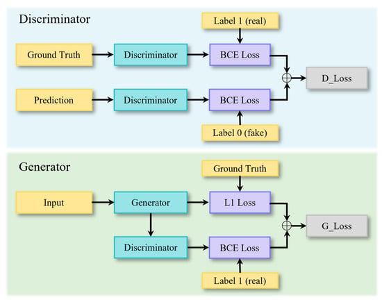
Figure 2. The structure of GAN.

During the discriminator training phase, the generator first creates a counterfeit prediction sequence without gradient updates. Subsequently, the discriminator distinguishes between the real label sequence and the generated sequence, outputting the probability of authenticity. To enhance the discriminator’s ability to distinguish, we used Binary Cross-Entropy (BCE) as the optimization objective. Specifically, the discriminator aims to maximize the recognition probability of real samples while minimizing the recognition probability of generated samples. Its loss function consists of two parts: the loss for real samples and the loss for generated samples:

$$L_D=L_{real}+L_{fake}=L_{BCE}\left(D\left(Y\right),1\right)+L_{BCE}\left(D\left(\widehat{Y}\right),0\right)$$

(7)

The BCE loss function is defined as:

$$L_{BCE}\left(y,\widehat{y}\right)=-\left[y\log \left(\widehat{y}\right)+\left(1-y\right)\log \left(1-\widehat{y}\right)\right]$$

(8)

where $y\in \left\{0,1\right\}$ represents the real label, and $\widehat{y}\in \left(0,1\right)$ represents the predicted probability, which can be either $D\left(Y\right)$ or $D\left(\widehat{Y}\right)$.

During the training phase of the generator, its goal is not only to minimize the prediction error with respect to the real sequence, but also to deceive the discriminator, thereby generating sequences that are closer to the real distribution. Specifically, the generator’s loss function consists of two parts: first, the prediction loss, which ensures the consistency between the generated sequence and the real sequence in terms of numerical values; second, the adversarial loss, which measures the discriminator’s judgment on the generated sequence. The overall loss is defined as:

$$L_G=L_{pred}+\lambda L_{adv}=L_{MAE}\left(G\left(X\right),Y\right)+\lambda L_{BCE}\left(D\left(G\left(X\right)\right),1\right)$$

(9)

where $L_{pred}$ represents the prediction error loss function, for which we use L1 Loss, and $L_{adv}$ denotes the adversarial loss. $\lambda \in \left[{10}^{-5},1.0\right]$ is a weight factor used to balance the trade-off between prediction accuracy and generation quality. This design provides stable gradients for the generator and helps mitigate potential oscillations during adversarial training. By minimizing $L_G$, the generator ensures that the predicted values are close to the real values while improving the distribution fitting ability of the generated sequence.

Through alternating training of the discriminator and the generator, the discriminator continuously enhances its ability to distinguish between real and generated samples, while the generator gradually learns to produce more realistic and reliable traffic flow prediction sequences. This process effectively improves the model’s prediction performance in complex traffic environments.

4. Methodology

The structure of the proposed SSGAN model consists of a generator and a discriminator. These two components interact through an adversarial training objective to mutually enhance each other: the generator is responsible for producing future traffic flow sequences based on historical traffic data and temporal features, while the discriminator aims to distinguish whether an input sequence corresponds to real traffic observations or synthetic predictions generated by the generator. Through this adversarial mechanism, the generator continuously improves the realism and plausibility of its outputs, whereas the discriminator progressively strengthens its discriminative capability, jointly driving the overall model to approximate the true distribution of traffic flow. To provide a clearer exposition of the model design, the following sections detail the architectures and optimization objectives of the generator and discriminator, respectively.

4.1. Generator

The overall architecture of the generator in the proposed SSGAN model is illustrated in Figure 3. First, the input sequence is standardized to eliminate differences in numerical ranges across traffic flow series and thereby improve training stability. The standardized input is then passed through an embedding layer, which maps both traffic flow and temporal features into a high-dimensional representation space.

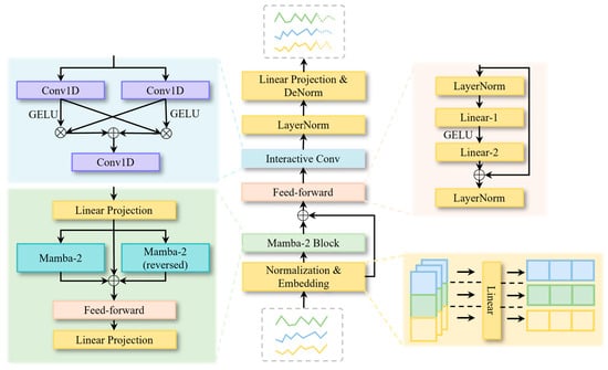
Figure 3. The framework of the generator.

Subsequently, the embedded representations are fed into a Mamba-2 Block, which consists of bidirectional Mamba-2 units, feed-forward layer, and linear layers, designed to efficiently capture long-term temporal dependencies. In this process, a residual connection is introduced by adding the output of the embedding layer to the output of the Mamba-2 Block, thereby enhancing feature transmission and stabilizing gradient propagation.

On this basis, the output is further transformed through a feed-forward layer for nonlinear feature learning, followed by an interactive convolution block that extracts local spatial features and fuses information from multiple receptive fields. Finally, the fused representations are processed by layer normalization and linear projection to map the high-dimensional features into the target prediction space, producing the final traffic flow forecasting results.

Embedding Layer. In traffic flow forecasting tasks, the raw input data are typically represented as a three-dimensional tensor $X\in {ℝ}^{B\times N\times S}$, where $B$ denotes the batch size, $N$ represents the number of detectors in the road network, and $S$ is the length of the time series. This input directly contains traffic flow values; however, due to its low dimensionality, it is insufficient to effectively capture complex temporal and spatial dependencies. To address this limitation, we introduced an embedding layer at the front end of the model, which projects the input features from the original space into a high-dimensional representation space through a linear transformation. Specifically, a fully connected layer is employed to perform the following mapping:

$$X=\mathrm{Dropout}\left(XW+b\right)$$

(10)

where $W\in {ℝ}^{T\times d}$ denotes the learnable projection matrix, $d$ is the embedding dimension, and $b$ represents the bias term.

Through this embedding layer, the raw traffic sequences are projected into a high-dimensional space, which not only strengthens the feature representation capacity but also provides a unified and trainable input representation for the subsequent spatiotemporal modeling modules.

Mamba-2 Module. The embedded representations are fed into the Mamba-2 block, which is built upon Structured State Space Duality (SSD). This design enables the model to capture both local and long-term dependencies with approximately linear computational complexity.

We considered a time-varying discrete SSM defined as follows:

$$h_t=\exp \left(A_t\right)\odot h_{t-1}+B_t{x}_t$$

(11)

$$y_t=C_t^T{h}_t$$

(12)

where $h_t\in {ℝ}^{B\times H\times N}$ denotes the hidden state, $H$ represents the number of heads, and $N$ is the state dimension; $x_t,y_t\in {ℝ}^{B\times H\times P}$, $P$ refers to the dimensionality of each head; $A_t\in {ℝ}^{B\times H}$; $B_t,C_t\in {ℝ}^{B\times H\times N}$ correspond to the input and output projections, respectively, $\odot$ denotes the element-wise product.

Direct temporal recursion suffers from low parallelism and numerical instability when modeling long sequences. To address this issue, Mamba-2 reformulates long-sequence recurrence into a combination of intra-block parallelism and inter-block lightweight recurrence through block partitioning and low-rank decomposition [18]. Specifically, a sequence of length $L$ is divided into $C=L/l$ blocks, and the input is rearranged into $x\in {ℝ}^{B\times C\times l\times H\times P}$. Within each block $c$, a decay kernel (a lower-triangular structure) is defined as follows:

$$L_c\left[\mathcal{l},s\right]=\exp \left({\displaystyle \sum _{k=s}^{\mathcal{l}-1}{A}_{c,k}}\right),\mathcal{l}>s$$

(13)

where $\mathcal{l},s$ indicates the position within the block, and $A_{c,k}$ represents the decay parameter at position $k$ of block $c$.

The computation of the diagonal block is formulated as follows, which corresponds to block-diagonal operations that can be executed fully in parallel within each block:

$$Y_{c,\mathcal{l}}^{diag}={\displaystyle \sum _{s<\mathcal{l}}{C}_{c,\mathcal{l}}\odot B_{c,s}\odot L_c\left[\mathcal{l},s\right]\odot x_{c,s}}$$

(14)

The compressed state at the end of each block is then computed as:

$$states\left[c\right]={\displaystyle \sum _{\mathcal{l}=1}^l{B}_{c,\mathcal{l}}\odot \exp \left({\displaystyle \sum _{k=\mathcal{l}+1}^l{A}_{c,k}}\right)\odot x_{c,\mathcal{l}}}$$

(15)

where $states\left[c\right]\in {ℝ}^{B\times H\times N}$ aggregates the inputs at all positions $\mathcal{l}$ within block $c$, decayed to the end of the block. $states\left[0\right]$ serves as an optional initial sequence state, which defaults to zero if not specified.

The inter-block recurrence is computed as follows:

$${\tilde{h}}_c={\displaystyle \sum _{k=1}^{c-1}\exp \left({\displaystyle \sum _{\mathcal{l}=1}^l{A}_{k,\mathcal{l}}}\right)\odot states\left[k\right]}$$

(16)

The computation from state to output is defined as:

$$Y_{c,\mathcal{l}}^{off}=C_{c,\mathcal{l}}\odot {\tilde{h}}_c\odot \exp \left({\displaystyle \sum _{k=1}^{\mathcal{l}}{A}_{c,k}}\right)$$

(17)

Finally, the overall output is obtained as the sum of two components:

$$Y=Y^{diag}+Y^{off}$$

(18)

Through the above mechanism, Mamba-2 achieves linear complexity when modeling long sequences. However, if relying solely on unidirectional accumulation, information transmission may suffer from latency. To address this issue, we employed a bidirectional Mamba-2 structure in the generator, where the forward and backward state evolutions are computed separately and subsequently fused along the feature dimension. By introducing this bidirectional design, the model can simultaneously account for the influence propagated from the past to the present as well as the reverse constraints traced back from the future to the present, thereby capturing more comprehensive global semantics. This design enables the model to more effectively learn bidirectional temporal dependencies in traffic flow, offering significant advantages for long-horizon forecasting and the modeling of complex traffic patterns.

Feed-Forward Layer. This layer is designed to perform nonlinear transformation and feature recombination on the high-dimensional representations of nodes, thereby enhancing the expressive power of the model. The structure consists of two linear transformations, with a nonlinear activation function applied in between to introduce nonlinearity:

$$X_1=\mathrm{Dropout}\left(\sigma \left(\mathrm{LayerNorm}\left(X\right)\cdot W_1+b_1\right)\right)$$

(19)

$$X_2=\mathrm{Dropout}\left(X_1\cdot W_2+b_2\right)$$

(20)

where $W_1\in {ℝ}^{d\times 4d}$ and $W_2\in {ℝ}^{4d\times d}$ denote the linear transformation matrices for dimensionality expansion and reduction, respectively; $\sigma$ is the GELU activation function; and LayerNorm represents the layer normalization operation.

Finally, residual connection and normalization are applied as follows:

$$X=\mathrm{LayerNorm}\left(X+X_2\right)$$

(21)

Interactive Convolution Block. In traffic flow forecasting, spatial correlations among nodes also play a crucial role. To this end, we adopted the interactive convolution block [24], which is specifically designed to capture spatial features across traffic network nodes. Given an input tensor $X\in {ℝ}^{B\times S\times N}$, the temporal dimension is treated as the convolutional channel, while the node dimension is regarded as the convolutional sequence, thereby enabling convolution operations along the spatial dimension of nodes.

In terms of structure, the interactive convolution block first applies two one-dimensional convolutions with kernel sizes of 1 and 3, respectively, to extract spatial features under different receptive fields:

$$X_1=\mathrm{Conv}1{\mathrm{d}}_1\left(X\right)$$

(22)

$$X_2=\mathrm{Conv}1{\mathrm{d}}_3\left(X\right)$$

(23)

To enhance the interaction between multi-scale convolutional features, an interaction mechanism is further introduced:

$$X_3=X_1\odot \mathrm{Dropout}\left(\sigma \left(X_2\right)\right)+X_2\odot \mathrm{Dropout}\left(\sigma \left(X_1\right)\right)$$

(24)

where $\sigma$ is the GELU activation function. This mechanism effectively fuses multi-scale spatial features, thereby enabling the model to better capture the complex dependencies among nodes in the road network.

Subsequently, the fused representations are processed through layer normalization and a one-dimensional convolution to project them back to the original channel dimension:

$$Y=\mathrm{Conv}1{\mathrm{d}}_1\left(\mathrm{LayerNorm}\left(X_3\right)\right)$$

(25)

Finally, a linear layer is applied to adjust the output dimensionality, followed by de-normalization, yielding the predicted traffic flow values.

4.2. Discriminator

The objective of the discriminator is to distinguish between real traffic flow data and the predictions generated by the generator. Unlike conventional discriminators that operate directly on time-domain sequences, we propose a frequency-domain-based discriminator to enhance its ability to capture periodic patterns in traffic flow. In real-world operations, traffic flow often exhibits clear periodic patterns (e.g., morning and evening peaks), which are difficult to explicitly capture in the time domain. By mapping the data to the frequency domain via the Fourier transform, these periodic characteristics can be more clearly represented, enabling the discriminator to more effectively distinguish real samples from generated ones.

Specifically, given an input tensor $X\in {ℝ}^{B\times N\times T}$, the temporal dimension is first transformed using Fast Fourier Transform (FFT):

$$X_{fft}=\mathrm{FFT}\left(X\right)$$

(26)

from which the real part $X_{real}$ and the imaginary part $X_{imag}$ are extracted. These components are then concatenated along the channel dimension to form the composite input feature:

$$X_{concat}=\mathrm{concat}\left(X_{real},X_{imag}\right)\in {ℝ}^{B\times 2N\times T}$$

(27)

Building on this, to further enhance the model’s ability to extract features at different temporal scales, a Multi-Scale Convolution module is introduced, as illustrated in Figure 4. This module applies one-dimensional convolutions with kernel sizes of 3, 5, and 7 to extract features at multiple receptive fields:

$$H_k=\sigma \left(\mathrm{Conv}1{\mathrm{d}}_k\left(X_{concat}\right)\right),k\in \left\{3,5,7\right\}$$

(28)

where $\sigma$ is the LeakyReLU activation function. The multi-scale features are then concatenated to obtain a combined representation:

$$H=\mathrm{Concat}\left(H_3,H_5,H_7\right)$$

(29)

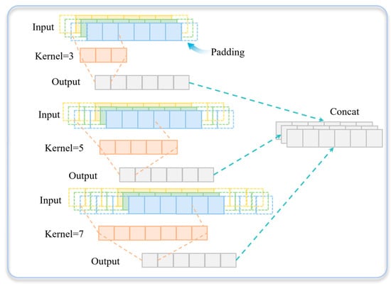
Figure 4. The framework of the discriminator.

To remove redundancy and restore the original number of node channels, a one-dimensional convolution with a kernel size of 1 is applied for feature compression:

$$Z=\mathrm{Conv}1{\mathrm{d}}_1\left(H\right)$$

(30)

5. Experiments

5.1. Datasets and Baselines

Experiments were conducted on four publicly available traffic datasets to evaluate the performance of the proposed SSGAN model. The PEMS datasets [36] collect traffic flow data from various regions of California highways and include four subsets: PEMS03, PEMS04, PEMS07, and PEMS08. These datasets cover selected months between 2017 and 2018. These datasets differ in spatial coverage, network density, and temporal length, providing heterogeneous traffic patterns that test the model’s ability to capture both short-term fluctuations and long-term dependencies. PEMS03 and PEMS04 primarily cover urban freeways in the San Francisco Bay Area, while PEMS07 and PEMS08 correspond to denser freeway networks in the Los Angeles area.

The statistical details of the datasets are summarized in Table 1, where Nodes denotes the number of detectors in each dataset, Dataset Size indicates the split proportions for the training, validation, and testing sets, and Frequency represents the sampling interval. These datasets provide a comprehensive benchmark for assessing the generalization ability and modeling effectiveness of the proposed model across different traffic prediction scenarios.

Table 1. Statistical description of datasets.

Dataset	Nodes	Time Steps	Dataset Size	Frequency
PEMS03	358	26,209	6:2:2	5 min
PEMS04	307	16,992	6:2:2	5 min
PEMS07	883	28,224	6:2:2	5 min
PEMS08	170	17,856	6:2:2	5 min

We selected seven baseline models, along with GL-SSD, for comparison:

• Mamba-based model. S-Mamba is built upon the Mamba model and efficiently captures sequential dependencies through linear encoding and feed-forward networks [28].
• Transformer-based models. iTransformer applies attention mechanisms along the variable dimension by transposing the input, modeling multivariate correlations while leveraging feed-forward networks for nonlinear representation learning [10]. Crossformer employs a dimension-segment-wise embedding to preserve temporal and variable information and integrates a two-stage attention mechanism to simultaneously model cross-time and cross-dimension dependencies [8].
• Linear models. TiDE combines an MLP-based encoder–decoder architecture with nonlinear mapping and covariate handling to achieve high-accuracy long-term time series forecasting with fast inference [37]. RLinear efficiently captures periodic features using linear mapping, invertible normalization, and channel-independent mechanisms [38]. DLinear, with its simple linear structure, reveals the temporal information loss issue inherent in Transformer-based models for long-term forecasting [22].
• Convolution-based model. TimesNet transforms one-dimensional time series into a set of two-dimensional tensors based on multiple periodicities, decomposing complex temporal variations into intra-period and inter-period changes, which are then modeled efficiently using 2D convolution kernels [39].

5.2. Forecasting Results

All prediction experiments were conducted using the PyTorch 2.3.1 framework on an NVIDIA GeForce RTX 4090 GPU. The Adam optimizer was employed, with the generator parameters and trainable adversarial weights optimized jointly, while the discriminator was optimized separately. A dynamic learning rate schedule was applied, decaying according to the training epoch. The loss function was the L1 Loss, the batch size was set to 32, and an early stopping strategy with a patience of 3 epochs was adopted. For all baseline models, hyperparameters were configured according to the original papers or official implementations. The input sequence length for all prediction models was set to 96 time steps, and the prediction horizons were set to $\left\{12,24,48,96\right\}$ time steps.

The prediction results across all forecast horizons for the PEMS datasets are presented in Table 2, where red indicates the best-performing results, and avg represents the average over four prediction horizons. The proposed SSGAN achieved the best performance in most settings for both MSE and MAE, and consistently outperformed other models in the avg metrics across all datasets, demonstrating its robustness and consistency across different horizons and datasets. As the prediction horizon increased, errors for all methods rose; however, the error growth of SSGAN was notably smaller. This advantage was particularly pronounced in long-horizon settings (e.g., 48 or 96 time steps), indicating the model’s superior ability to capture long-term dependencies and complex spatiotemporal patterns.

Table 2. Prediction results on the PEMS datasets.

Models		SSGAN (Ours)		S-Mamba (2025)		iTransformer (2024)		RLinear (2023)		Crossformer (2023)		TiDE (2023)		TimesNet (2023)		DLinear (2023)
Metric		MSE	MAE	MSE	MAE	MSE	MAE	MSE	MAE	MSE	MAE	MSE	MAE	MSE	MAE	MSE	MAE
PEMS03	12	0.072	0.174	0.065	0.169	0.071	0.174	0.126	0.236	0.090	0.203	0.178	0.305	0.085	0.192	0.122	0.243
	24	0.086	0.191	0.087	0.196	0.093	0.201	0.246	0.334	0.121	0.240	0.257	0.371	0.118	0.223	0.201	0.317
	48	0.120	0.225	0.133	0.243	0.125	0.236	0.551	0.529	0.202	0.317	0.379	0.463	0.155	0.260	0.333	0.425
	96	0.147	0.248	0.201	0.305	0.164	0.275	1.057	0.787	0.262	0.367	0.490	0.539	0.228	0.317	0.457	0.515
	Avg	0.106	0.210	0.122	0.228	0.113	0.221	0.495	0.472	0.169	0.281	0.326	0.419	0.147	0.248	0.278	0.375
PEMS04	12	0.070	0.169	0.076	0.180	0.078	0.183	0.138	0.252	0.098	0.218	0.219	0.340	0.087	0.195	0.148	0.272
	24	0.079	0.179	0.084	0.193	0.095	0.205	0.258	0.348	0.131	0.256	0.292	0.398	0.103	0.215	0.224	0.340
	48	0.091	0.193	0.115	0.224	0.120	0.233	0.572	0.544	0.205	0.326	0.409	0.478	0.136	0.250	0.355	0.437
	96	0.103	0.207	0.137	0.248	0.150	0.262	1.137	0.820	0.402	0.457	0.492	0.532	0.190	0.303	0.452	0.504
	Avg	0.086	0.187	0.103	0.211	0.111	0.221	0.526	0.491	0.209	0.314	0.353	0.437	0.129	0.241	0.295	0.388
PEMS07	12	0.068	0.152	0.063	0.159	0.067	0.165	0.118	0.235	0.094	0.200	0.173	0.304	0.082	0.181	0.115	0.242
	24	0.076	0.167	0.081	0.183	0.088	0.190	0.242	0.341	0.139	0.247	0.271	0.383	0.101	0.204	0.210	0.329
	48	0.096	0.185	0.093	0.192	0.110	0.215	0.562	0.541	0.311	0.369	0.446	0.495	0.134	0.238	0.398	0.458
	96	0.122	0.203	0.117	0.217	0.139	0.245	1.096	0.795	0.396	0.442	0.628	0.577	0.181	0.279	0.594	0.553
	Avg	0.091	0.177	0.089	0.188	0.101	0.204	0.504	0.478	0.235	0.315	0.380	0.440	0.124	0.225	0.329	0.395
PEMS08	12	0.139	0.182	0.076	0.178	0.079	0.182	0.133	0.247	0.165	0.214	0.227	0.343	0.112	0.212	0.154	0.276
	24	0.162	0.200	0.104	0.209	0.115	0.219	0.249	0.343	0.215	0.260	0.318	0.409	0.141	0.238	0.248	0.353
	48	0.189	0.218	0.167	0.228	0.186	0.235	0.569	0.544	0.315	0.355	0.497	0.510	0.198	0.283	0.440	0.470
	96	0.217	0.237	0.245	0.280	0.221	0.267	1.166	0.814	0.377	0.397	0.721	0.592	0.320	0.351	0.674	0.565
	Avg	0.177	0.209	0.148	0.224	0.150	0.226	0.529	0.487	0.268	0.307	0.441	0.464	0.193	0.271	0.379	0.416
1st Count		11	18	9	2	0	0	0	0	0	0	0	0	0	0	0	0

Compared with strong baselines such as S-Mamba and iTransformer, SSGAN demonstrated competitive performance for short-term horizons and maintained a stable advantage over longer horizons. Other baselines, including DLinear, RLinear, Crossformer, TiDE, and TimesNet, generally underperformed, with their disadvantages becoming more pronounced for long-term predictions. Moreover, the rankings of MSE and MAE were largely consistent, indicating that the improvement brought by SSGAN was not merely due to the reduction in a few extreme errors, but reflects an overall improvement in the error distribution. Overall, SSGAN achieved state-of-the-art performance and exhibited stronger generalization capability for traffic flow forecasting tasks.

To further evaluate the ability of the models to preserve the dynamic structure of traffic flow in long-term prediction tasks, we computed the Signal-to-Noise Ratio (SNR) for a 96-step prediction horizon, as shown in Table 3. A higher SNR indicates that the model better retains the temporal variations of the original signal in the generated sequences, reducing information loss caused by over-smoothing or noise.

Table 3. Signal-to-noise ratio results.

Model	PEMS03	PEMS04	PEMS07	PEMS08
SSGAN	17.496	18.841	21.287	19.583
S-Mamba	6.418	19.558	22.223	21.333
iTransformer	19.135	19.520	20.909	17.514

The results show that the proposed SSGAN achieved consistently high SNR values across all four datasets, demonstrating its effectiveness in maintaining the overall dynamic trends of traffic flow in long-term forecasting.

Compared with S-Mamba, although SSGAN exhibited slightly lower SNR on PEMS04, PEMS07, and PEMS08 (with differences of approximately 0.3–2 dB), it significantly outperformed S-Mamba on PEMS03. This result indicates that SSGAN can maintain high signal fidelity and prediction stability even in scenarios with stronger noise interference and more complex network structures. Furthermore, compared with iTransformer, SSGAN achieved higher SNR values on PEMS07 and PEMS08, demonstrating its capability to preserve global dynamics in large-scale traffic networks and long-horizon prediction tasks.

To provide a more intuitive illustration of the model’s predictive performance, we plotted the forecasted traffic flows of the three best-performing models, as shown in Figure 5 and Figure 6. It can be observed that all methods generally followed the overall trend of the ground truth; however, significant differences existed in fitting accuracy at traffic peaks and troughs. Compared with iTransformer and S-Mamba, the proposed SSGAN more closely tracked the true curve during abrupt traffic fluctuations, exhibiting smaller prediction delays and deviations. Moreover, SSGAN maintained high prediction accuracy in stable periods, demonstrating superior stability and robustness.

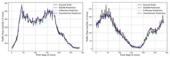
Figure 5. The 96-step traffic flow predictions on the PEMS03 (left) and PEMS04 (right) datasets.

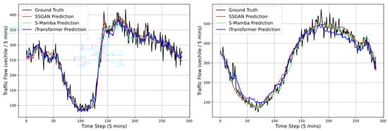
Figure 6. The 96-step traffic flow predictions on the PEMS07 (left) and PEMS08 (right) datasets.

5.3. Hyperparameter Experiments

We employed the Optuna framework for systematic hyperparameter optimization, using the tree-structured parzen estimator as the sampler. The optimization objective was to minimize the validation set loss, with MAE selected as the evaluation metric. For each prediction horizon, 100 trials were conducted, and the hyperparameter configuration corresponding to the best performance on the validation set was selected.

In designing the hyperparameter search space, both model complexity and computational feasibility were considered. The main parameters optimized included: embedding dimension selected from $\left\{32,64,128\right\}$; hidden layer dimension, state dimension, and the number of channels in the interactive convolution block chosen from $\left\{64,128,256\right\}$; multi-scale convolution channels selected from $\left\{32,64,128\right\}$, with kernel size combinations including $\left\{\left[3\right],\left[5\right],\left[7\right],\left[3,5\right],\left[3,7\right],\left[5,7\right],\left[3,5,7\right]\right\}$.

Additionally, to ensure reproducibility, all experiments used fixed random seeds, guaranteeing stability during model training and the comparability of results.

5.4. Ablation Study

To validate the effectiveness of key components in the proposed model, three sets of ablation experiments were designed to assess the impact of different modules on overall performance:

• Bidirectional Mamba-2 replaced with unidirectional: The bidirectional Mamba-2 module in the generator was replaced with a unidirectional structure to evaluate the contribution of bidirectional temporal dependency modeling to long-sequence prediction performance.
• Removal of the interactive convolution block: The interactive convolution block in the generator was removed to examine its role in feature fusion.
• Removal of the adversarial framework (generator-only): The discriminator in the GAN framework was completely removed, leaving only the generator for prediction, in order to analyze the importance of the adversarial mechanism in alleviating over-smoothing and improving the capture of fine-grained temporal patterns.

Table 4 presents the results of the ablation experiments. Replacing the bidirectional Mamba-2 with a unidirectional variant led to increases in both MSE and MAE across all prediction horizons on the PEMS04, PEMS07, and PEMS08 datasets. The most notable increase occurred on PEMS08 for the 96-step prediction horizon, where MSE and MAE increased by 3.69% and 2.95%, respectively. This demonstrates that the bidirectional structure provides an advantage in capturing both past and future temporal dependencies, contributing to improved accuracy for long-sequence predictions.

Table 4. Ablation study results.

Models	Horizon	PEMS03		PEMS04		PEMS07		PEMS08
		MSE	MAE	MSE	MAE	MSE	MAE	MSE	MAE
SSGAN	12	0.072	0.174	0.070	0.169	0.068	0.152	0.139	0.182
	24	0.086	0.191	0.079	0.179	0.076	0.167	0.162	0.200
	48	0.120	0.225	0.091	0.193	0.096	0.185	0.189	0.218
	96	0.147	0.248	0.103	0.207	0.122	0.203	0.217	0.237
	Avg	0.106	0.210	0.086	0.187	0.091	0.177	0.177	0.209
Bidirectional Mamba-2 replaced with unidirectional	12	0.072	0.174	0.070	0.169	0.070	0.154	0.140	0.186
	24	0.086	0.192	0.079	0.180	0.077	0.167	0.159	0.200
	48	0.117	0.223	0.093	0.196	0.099	0.191	0.190	0.220
	96	0.149	0.252	0.104	0.208	0.124	0.207	0.225	0.244
	Avg	0.106	0.210	0.087	0.188	0.093	0.180	0.179	0.213
Removal of the interactive convolution block	12	0.071	0.173	0.070	0.169	0.064	0.153	0.129	0.184
	24	0.087	0.194	0.078	0.179	0.078	0.169	0.162	0.202
	48	0.118	0.223	0.090	0.192	0.094	0.186	0.189	0.222
	96	0.160	0.256	0.102	0.207	0.126	0.208	0.214	0.241
	Avg	0.109	0.212	0.085	0.187	0.091	0.179	0.174	0.212
Removal of the adversarial framework	12	0.074	0.176	0.070	0.169	0.071	0.154	0.133	0.182
	24	0.085	0.190	0.080	0.180	0.079	0.167	0.162	0.201
	48	0.120	0.223	0.093	0.196	0.097	0.189	0.188	0.219
	96	0.152	0.252	0.104	0.207	0.121	0.203	0.227	0.245
	Avg	0.108	0.210	0.087	0.188	0.092	0.178	0.178	0.212

Removing the interactive convolution block resulted in performance comparable to the full model for short-term predictions, but significantly degraded performance for long-term horizons. For example, in the 96-step prediction on PEMS03, the MSE increased from 0.147 to 0.160. This indicates that the interactive convolution block plays a critical role in fusing multi-scale features along the spatial dimension, and its absence weakens the model’s ability to capture spatial correlations.

When the GAN framework was removed and only the generator was used for prediction, the average prediction errors increased across all four datasets. In particular, for the 96-step prediction on PEMS08, MSE rose from 0.217 to 0.227, and MAE increased from 0.237 to 0.245. This highlights the indispensable role of adversarial learning in mitigating over-smoothing and restoring fine-grained fluctuations in traffic flow.

In summary, these three ablation studies fully validate the importance of the bidirectional state-space structure, the interactive convolution block, and the adversarial framework in the proposed model.

To evaluate whether the proposed SSGAN model can alleviate the over-smoothing problem in long-term traffic flow prediction, we visualized the 96-step predictions on the PEMS03 and PEMS08 datasets. Specifically, each prediction matrix was treated as a feature representation of traffic nodes. We first reduced the high-dimensional representations to three dimensions using t-distributed stochastic neighbor embedding and then projected them onto a unit sphere to preserve the overall distribution structure.

As shown in Figure 7 and Figure 8, in the generator-only model (right panels), most node features were highly concentrated, indicating severe over-smoothing. In contrast, the SSGAN model (left panels) produced a more widely spread distribution of node features, reflecting richer and more diverse representations. This visualization demonstrates that the SSGAN model effectively mitigates over-smoothing, thereby better capturing the complex spatiotemporal variations of traffic flow.

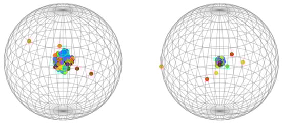
Figure 7. Visualization of over-smoothing alleviation by SSGAN on the PEMS03 dataset.

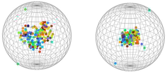
Figure 8. Visualization of over-smoothing alleviation by SSGAN on the PEMS08 dataset.

5.5. Model Efficiency

On the PEMS04 dataset, we conducted an efficiency evaluation of different models under the setting of a prediction horizon of 96 and a batch size of 32, measuring their prediction errors, average training time, and memory usage. As shown in Table 5, SSGAN achieved the lowest MSE and MAE, while also delivering the fastest training speed (60 ms/iter) with a memory consumption only slightly higher than that of DLinear, demonstrating significant advantages in both accuracy and efficiency. S-Mamba attained a prediction accuracy comparable to SSGAN, but its training speed was substantially slower and its memory usage was higher, making it less efficient overall. iTransformer exhibited further degradation in accuracy, with training speed and memory consumption at moderate levels. Overall, SSGAN achieved superior prediction performance while substantially reducing computational and memory overhead, highlighting its potential for practical deployment.

Table 5. Efficiency results.

Model	MAE	MSE	Training Speed (ms/iter)	Memory Usage (GB)
SSGAN	0.207	0.103	60	0.48
S-Mamba	0.248	0.137	486	8.75
iTransformer	0.262	0.150	161	6.07
Crossformer	0.457	0.402	543	41.07
TimesNet	0.303	0.190	1146	10.53
DLinear	0.504	0.452	92	0.13

6. Conclusions

We proposed SSGAN, a novel generative adversarial framework for long-term traffic flow forecasting, which integrates a state-space-based generator with multi-scale convolutional discriminators. By jointly modeling temporal dependencies and spatial correlations, the proposed method effectively alleviates the over-smoothing issue commonly observed in long-horizon time series prediction and enhances the model’s ability to capture fine-grained spatiotemporal dynamics.

Extensive experiments on four real-world PEMS datasets demonstrated that SSGAN consistently outperformed a wide range of strong baselines, including Mamba-, Transformer-, linear-, and convolution-based models. In particular, SSGAN achieved state-of-the-art accuracy across different horizons, with performance advantages becoming more pronounced under long prediction lengths. Visualization analyses further confirmed that SSGAN preserves node-level heterogeneity and mitigates over-smoothing in comparison to generator-only models. Moreover, efficiency experiments highlighted that SSGAN not only delivers superior predictive accuracy, but also reduces the computational and memory costs, underscoring its potential for large-scale deployment in intelligent transportation systems.

While the current work focused primarily on improving the accuracy and efficiency of long-term traffic flow prediction, the proposed framework provides a foundation for future studies to explore practical applications, such as congestion management, urban traffic analytics, and traffic risk assessment. Extending SSGAN to these applied scenarios will be an interesting direction for future research.

References

- Wang, R.; Lin, W.; Ren, G.; Cao, Q.; Zhang, Z.; Deng, Y. Interaction-Aware Vehicle Trajectory Prediction Using Spatial-Temporal Dynamic Graph Neural Network. Knowl.-Based Syst. 2025, 327, 114187. [Google Scholar] [CrossRef]
- Zhang, J.; Huang, D.; Liu, Z.; Zheng, Y.; Han, Y.; Liu, P.; Huang, W. A data-driven optimization-based approach for freeway traffic state estimation based on heterogeneous sensor data fusion. Transp. Res. Part E Logist. Transp. Rev. 2024, 189, 103656. [Google Scholar] [CrossRef]
- Huang, D.; Zhang, J.; Liu, Z.; Liu, R. Prescriptive analytics for freeway traffic state estimation by multi-source data fusion. Transp. Res. Part E Logist. Transp. Rev. 2025, 198, 104105. [Google Scholar] [CrossRef]
- Zhao, Y.; Hua, X.; Yu, W.; Lin, W.; Wang, W.; Zhou, Q. Safety and efficiency-oriented adaptive strategy controls for connected and automated vehicles in unstable communication environment. Accid. Anal. Prev. 2025, 220, 108121. [Google Scholar] [CrossRef] [PubMed]
- Huang, D.; Zhang, J.; Liu, Z.; He, Y.; Liu, P. A novel ranking method based on semi-SPO for battery swapping allocation optimization in a hybrid electric transit system. Transp. Res. Part E Logist. Transp. Rev. 2024, 188, 103611. [Google Scholar] [CrossRef]
- Vaswani, A.; Shazeer, N.; Parmar, N.; Uszkoreit, J.; Jones, L.; Gomez, A.N.; Kaiser, L.; Polosukhin, I. Attention is all you need. Adv. Neural Inf. Process. Syst. 2017, 30, 5999–6009. [Google Scholar] [CrossRef]
- Zhou, T.; Ma, Z.; Wen, Q.; Wang, X.; Sun, L.; Jin, R. Fedformer: Frequency enhanced decomposed transformer for long-term series forecasting. In Proceedings of the International Conference on Machine Learning, Honolulu, HI, USA, 23–29 July 2022; pp. 27268–27286. [Google Scholar]
- Zhang, Y.; Yan, J. Crossformer: Transformer utilizing cross-dimension dependency for multivariate time series forecasting. In Proceedings of the Eleventh International Conference on Learning Representations, Kigali, Rwanda, 1–5 May 2023. [Google Scholar]
- Nie, Y.; Nguyen, N.H.; Sinthong, P.; Kalagnanam, J. A Time Series is Worth 64 Words: Long-term Forecasting with Transformers. In Proceedings of the Eleventh International Conference on Learning Representations, Kigali, Rwanda, 1–5 May 2023. [Google Scholar]
- Liu, Y.; Hu, T.; Zhang, H.; Wu, H.; Wang, S.; Ma, L.; Long, M. iTransformer: Inverted Transformers Are Effective for Time Series Forecasting. In Proceedings of the Twelfth International Conference on Learning Representations, Vienna, Austria, 7–11 May 2024. [Google Scholar]
- Luo, Q.; He, S.; Han, X.; Wang, Y.; Li, H. LSTTN: A long-short term transformer-based spatiotemporal neural network for traffic flow forecasting. Knowl. Based Syst. 2024, 293, 111637. [Google Scholar] [CrossRef]
- Xiao, J.; Long, B. A multi-channel spatial-temporal transformer model for traffic flow forecasting. Inf. Sci. 2024, 671, 120648. [Google Scholar] [CrossRef]
- Fang, Y.; Liang, Y.; Hui, B.; Shao, Z.; Deng, L.; Liu, X.; Jiang, X.; Zheng, K. Efficient large-scale traffic forecasting with transformers: A spatial data management perspective. In Proceedings of the 31st ACM SIGKDD Conference on Knowledge Discovery and Data Mining V. 1, Toronto, ON, Canada, 3–7 August 2025; pp. 307–317. [Google Scholar]
- Lu, J.; Yao, J.; Zhang, J.; Zhu, X.; Xu, H.; Gao, W.; Xu, C.; Xiang, T.; Zhang, L. Soft: Softmax-free transformer with linear complexity. Adv. Neural Inf. Process. Syst. 2021, 34, 21297–21309. [Google Scholar]
- Gu, A.; Dao, T.; Ermon, S.; Rudra, A.; Ré, C. Hippo: Recurrent memory with optimal polynomial projections. Adv. Neural Inf. Process. Syst. 2020, 33, 1474–1487. [Google Scholar]
- Gu, A.; Goel, K.; Ré, C. Efficiently modeling long sequences with structured state spaces. arXiv 2021, arXiv:2111.00396. [Google Scholar]
- Gu, A.; Dao, T. Mamba: Linear-time sequence modeling with selective state spaces. arXiv 2023, arXiv:2312.00752. [Google Scholar] [CrossRef]
- Dao, T.; Gu, A. Transformers are SSMs: Generalized models and efficient algorithms through structured state space duality. arXiv 2024, arXiv:2405.21060. [Google Scholar] [CrossRef]
- Sun, Y.; Xie, Z.; Chen, D.; Eldele, E.; Hu, Q. Hierarchical classification auxiliary network for time series forecasting. Proc. AAAI Conf. Artif. Intell. 2025, 39, 20743–20751. [Google Scholar] [CrossRef]
- Goodfellow, I.J.; Pouget-Abadie, J.; Mirza, M.; Xu, B.; Warde-Farley, D.; Ozair, S.; Bengio, Y. Generative adversarial nets. Adv. Neural Inf. Process. Syst. 2014, 27, 1–9. [Google Scholar] [CrossRef]
- Wen, Q.; Zhou, T.; Zhang, C.; Chen, W.; Ma, Z.; Yan, J.; Sun, L. Transformers in time series: A survey. In Proceedings of the Thirty-Second International Joint Conference on Artificial Intelligence, Macao, China, 19–25 August 2023; pp. 6778–6786. [Google Scholar]
- Zeng, A.; Chen, M.; Zhang, L.; Xu, Q. Are transformers effective for time series forecasting? Proc. AAAI Conf. Artif. Intell. 2023, 37, 11121–11128. [Google Scholar] [CrossRef]
- Bi, J.; Zhang, X.; Yuan, H.; Zhang, J.; Zhou, M. A hybrid prediction method for realistic network traffic with temporal convolutional network and LSTM. IEEE Trans. Autom. Sci. Eng. 2021, 19, 1869–1879. [Google Scholar] [CrossRef]
- Eldele, E.; Ragab, M.; Chen, Z.; Wu, M.; Li, X. TSLANet: Rethinking transformers for time series representation learning. arXiv 2024, arXiv:2404.08472. [Google Scholar] [CrossRef]
- Su, J.; Xie, D.; Duan, Y.; Zhou, Y.; Hu, X.; Duan, S. MDCNet: Long-term time series forecasting with mode decomposition and 2D convolution. Knowl.-Based Syst. 2024, 299, 111986. [Google Scholar] [CrossRef]
- Reza, S.; Ferreira, M.C.; Machado, J.J.M.; Tavares, J.M.R. Enhancing intelligent transportation systems with a more efficient model for long-term traffic predictions based on an attention mechanism and a residual temporal convolutional network. Neural Netw. 2025, 192, 107897. [Google Scholar] [CrossRef]
- Lee, M.; Yoon, H.; Kang, M. CASA: CNN Autoencoder-based Score Attention for Efficient Multivariate Long-term Time-series Forecasting. arXiv 2025, arXiv:2505.02011. [Google Scholar]
- Wang, Z.; Kong, F.; Feng, S.; Wang, M.; Yang, X.; Zhao, H.; Wang, D.; Zhang, Y. Is mamba effective for time series forecasting? Neurocomputing 2025, 619, 129178. [Google Scholar] [CrossRef]
- Lin, W.; Zhang, Z.; Ren, G.; Zhao, Y.; Ma, J.; Cao, Q. MGCN: Mamba-integrated spatiotemporal graph convolutional network for long-term traffic forecasting. Knowl.-Based Syst. 2025, 309, 112875. [Google Scholar] [CrossRef]
- Cao, J.; Sheng, X.; Zhang, J.; Duan, Z. iTransMamba: A lightweight spatio-temporal network based on long-term traffic flow forecasting. Knowl.-Based Syst. 2025, 317, 113416. [Google Scholar] [CrossRef]
- Hamad, M.; Mabrok, M.; Zorba, N. MCST-Mamba: Multivariate Mamba-Based Model for Traffic Prediction. arXiv 2025, arXiv:2507.03927. [Google Scholar]
- Wang, X.; Cao, J.; Zhao, T.; Zhang, B.; Chen, G.; Li, Z.; Chen, H.; Tu, W.; Li, Q. ST-Camba: A decoupled-free spatiotemporal graph fusion state space model with linear complexity for efficient traffic forecasting. Inf. Fusion 2025, 126, 103495. [Google Scholar] [CrossRef]
- Zhang, L.; Wu, J.; Shen, J.; Chen, M.; Wang, R.; Zhou, X.; Xu, C.; Yao, Q.; Wu, Q. SATP-GAN: Self-attention based generative adversarial network for traffic flow prediction. Transp. B Transp. Dyn. 2021, 9, 552–568. [Google Scholar] [CrossRef]
- Khaled, A.; Elsir, A.M.T.; Shen, Y. TFGAN: Traffic forecasting using generative adversarial network with multi-graph convolutional network. Knowl.-Based Syst. 2022, 249, 108990. [Google Scholar] [CrossRef]
- Zhang, Z.; Cao, Q.; Lin, W.; Song, J.; Chen, W.; Ren, G. Estimation of arterial path flow considering flow distribution consistency: A data-driven semi-supervised method. Systems 2024, 12, 507. [Google Scholar] [CrossRef]
- Chen, C.; Petty, K.; Skabardonis, A.; Varaiya, P.; Jia, Z. Freeway performance measurement system: Mining loop detector data. Transp. Res. Rec. 2001, 1748, 96–102. [Google Scholar] [CrossRef]
- Das, A.; Kong, W.; Leach, A.; Mathur, S.; Sen, R.; Yu, R. Long-term forecasting with tide: Time-series dense encoder. arXiv 2023, arXiv:2304.08424. [Google Scholar]
- Li, Z.; Qi, S.; Li, Y.; Xu, Z. Revisiting long-term time series forecasting: An investigation on linear mapping. arXiv 2023, arXiv:2305.10721. [Google Scholar] [CrossRef]
- Wu, H.; Hu, T.; Liu, Y.; Zhou, H.; Wang, J.; Long, M. TimesNet: Temporal 2D-Variation Modeling for General Time Series Analysis. In Proceedings of the Eleventh International Conference on Learning Representations, Kigali, Rwanda, 1–5 May 2023. [Google Scholar]
Disclaimer/Publisher’s Note: The statements, opinions and data contained in all publications are solely those of the individual author(s) and contributor(s) and not of MDPI and/or the editor(s). MDPI and/or the editor(s) disclaim responsibility for any injury to people or property resulting from any ideas, methods, instructions or products referred to in the content. |
© 2025 by the authors. Licensee MDPI, Basel, Switzerland. This article is an open access article distributed under the terms and conditions of the Creative Commons Attribution (CC BY) license (https://creativecommons.org/licenses/by/4.0/).