Article

Modeling Blockchain Investment in Data-Intensive Supply Chains: A Game-Theoretic Analysis of Power Structures

School of Transportation and Logistics, Southwest Jiaotong University, Chengdu 610031, China
*
Author to whom correspondence should be addressed.
Systems 2025, 13(11), 1029; https://doi.org/10.3390/systems13111029
Submission received: 22 October 2025 / Revised: 12 November 2025 / Accepted: 14 November 2025 / Published: 17 November 2025
(This article belongs to the Section Supply Chain Management)

Abstract

This study advances the hypothesis that supply chain power structure is a critical contingency factor for realizing investment value from integrating blockchain and big data. We develop a game-theoretic model of a two-tier supply chain to analyze investment decisions. The model examines cost–benefit dynamics under supplier-led, manufacturer-led, and balanced power structures and proposes a coordination mechanism to align incentives. Results demonstrate that power structure determines pricing and profit distribution, allowing the dominant party to capture a larger benefit share. Furthermore, power structure systematically interacts with technological performance: profitability increases with customer heterogeneity satisfaction and demand enhancement but can be eroded by a high technology cost coefficient that triggers disproportionate investment. We identify a critical investment cost threshold for achieving Pareto improvement. Finally, the demand premium from enhanced transparency ensures economic viability even when adoption increases prices. These insights offer strategic frameworks for blockchain investment tailored to specific power distributions.

1. Introduction

Contemporary supply chain management has entered an era defined by the technological collaboration of “big data + blockchain technology (BDBT)” [1]. BDBT constitutes a hybrid system that deeply integrates big data analysis technology (BDAT) with blockchain technology (BT), forming an organic whole rather than a simple combination of sequential upgrades [2]. Within this framework, BDAT and BT function synergistically: BDAT extracts insights from massive datasets to optimize decisions and enhance the efficiency of demand forecasting and inventory management [3], while blockchain provides a trusted, transparent, and automated execution environment for this data and its derived business logic through distributed ledgers and smart contracts [4,5]. For instance, Walmart’s blockchain traceability system can locate a product’s source in seconds and retrieve detailed item information within minutes [6]. BDBT thus creates a closed-loop value creation model, moving from “data insight” to “trusted execution.” Consequently, for enterprises that have already adopted BDAT, investing in BT presents a compelling strategic priority.
However, the decision to make this additional technological investment is often complicated by distortions arising from the supply chain’s power structure. In practice, realizing the full value of BT hinges on the collaborative integration of upstream and downstream data, such as material traceability and unified production process records [7]. This interdependence requires simultaneous investments from multiple supply chain members in complementary infrastructure, including standardized data interfaces and smart contract systems [8]. Yet, existing literature suggests that power asymmetries can trap such technology investments in a “Prisoner’s Dilemma” [9,10,11]. A dominant firm may leverage its bargaining power to shift investment costs onto others, while a subordinate partner may withhold cooperative investments due to perceived inequities in benefit distribution. The result is that BT implementation often fails to achieve full-chain connectivity, hindered by conflicting interests in revenue allocation.
The manifestation of this dilemma varies with the power configuration. In a supplier-dominated chain (e.g., involving specialized chip manufacturers), the powerful supplier may implicitly pass the costs of deploying blockchain nodes to manufacturers through wholesale pricing. Conversely, in manufacturer-dominated contexts (e.g., featuring large food producers), the manufacturer’s control over end-customer data can compel suppliers to bear the expenses of upstream traceability. In balanced power scenarios (e.g., alliances of comparable small and medium-sized enterprises), a “free-rider” mentality can raise the collective action threshold for collaborative investment.
Despite these structural challenges, existing research has primarily focused on the operational efficiency gains afforded by the technology itself [12,13,14,15], often overlooking the critical constraints that power structures impose on investment incentives. The variations in cost optimization, efficiency improvement, and revenue distribution across different structural arrangements remain underexplored, leading to a growing divergence between theoretical models of technological potential and their real-world application.
To address these research gaps, this study establishes three specific objectives:
  • To derive and compare the equilibrium strategies for BT investment under three distinct power structures within a BDAT environment.
  • To quantify the moderating effect of power structure on profit distribution among supply chain members.
  • To design effective contracts that can coordinate investment incentives and resolve the identified predicaments.
Guiding the model construction and analysis are the following core hypotheses:
H1: 
In a BDAT environment, achieving Pareto improvement through BT investment is contingent upon the investment cost falling below a critical threshold, which is itself moderated by the power structure.
H2: 
The power structure significantly influences profit distribution, with the dominant party expected to capture the majority of the incremental value created by BT investment.
H3: 
A properly designed coordination contract can enhance overall supply chain efficiency across different power structures, bringing its performance closer to the centralized decision-making optimum.
To achieve these objectives and test these hypotheses, this study constructs a game-theoretic model of a two-tier supply chain, integrating perspectives from transaction cost economics and the resource-based view. The model analyzes the investment decisions, profit variations, and supply chain performance of suppliers and manufacturers under three power configurations. This analysis reveals the moderating role of power structure on BT investment value and explores contractual coordination mechanisms. The conclusions are subsequently verified through numerical simulation.
The theoretical contribution of this research is threefold. First, it moves beyond treating blockchain as a universal solution by constructing a “power structure-contingent” investment decision theory for BDAT environments. Second, it elucidates how power dynamics systematically regulate the distribution of technological value. Finally, it enriches interdisciplinary research on technology, governance, and contract design in the context of supply chain digital transformation. Practically, the findings offer actionable insights—such as investment threshold benchmarks, pricing strategy adjustments, and negotiation frameworks—to assist firms in different power positions (leaders or followers) in making scientifically grounded investment decisions and fostering collaborative value creation in their transition from BDAT to BDBT.
The remainder of this paper is structured as follows. Section 2 reviews the relevant literature. Section 3 introduces the proposed model and benefit functions. Section 4 details the decision-making mechanism. Section 5 discusses model extensions. Section 6 presents the numerical analysis and managerial implications. Finally, Section 7 concludes by summarizing the key findings.

2. Literature Review

This section reviews the relevant literature through three subsections: (1) Supply Chain Power Structure and Decision-Making Behavior; (2) Blockchain’s Trust Mechanism and its Supply Chain Value; and (3) Investment Decisions for Supply Chain BDBT. A synthesis concludes the section to delineate the research gaps.

2.1. Supply Chain Power Structure and Decision-Making Behavior

The power structure of a supply chain is a core determinant of its members’ decision-making processes and has consequently attracted significant scholarly attention. Extensive research confirms that power configurations profoundly influence operational choices and profit distribution [16,17,18,19]. Seminal work by Choi [20] analyzed three non-cooperative game structures—Manufacturer–Stackelberg, Retailer–Stackelberg, and Nash equilibrium—establishing a foundational framework. Subsequent studies have explored this impact across various domains: Wang et al. [21] and Li and Mizuno [22] examined power structures in financing and operational strategies and dynamic pricing and inventory management, respectively.
Further refining this understanding, Tatarczak and Gola [23] developed a fuzzy logic-based multi-criteria framework for partner selection, effectively addressing subjectivity and uncertainty in horizontal cooperation. Jin et al. [24] investigated pricing and coordination in competitive recycling channels, finding that balanced power can enhance overall efficiency, facilitated by appropriate coordination mechanisms. Introducing behavioral factors, Shi et al. [25] demonstrated that empathy preference within poverty-alleviation e-commerce supply chains interacts with power structure to affect profit distribution and negotiations.
The consensus indicates that while dominant members often capture disproportionate benefits, overall supply chain efficiency can be maximized under a balanced Nash equilibrium [26]. For instance, a power shift towards retailers may enhance product sustainability but potentially reduce overall chain efficiency [26]. In agricultural supply chains, Lai et al. [27] modeled direct procurement as a constrained alliance game, showing that power asymmetry directly dictates profit division. Similarly, Gao et al. [28] confirmed the significant impact of power structure on pricing and performance in the power battery closed-loop supply chain.
In summary, while the extant literature robustly establishes the impact of power structure on traditional supply chain decisions, it pays insufficient attention to its differentiated effect on digital technology investment choices. Although a nascent stream of research has begun to place BT investment within different power structures to explore profit distribution [29,30,31], a systematic understanding of how power structures regulate the value of BT investment within a BDAT environment remains underdeveloped.

2.2. Blockchain’s Trust Mechanism and Its Supply Chain Value

BT is aptly characterized as a “trust machine” with significant applicability to supply chain management. It enables comprehensive end-to-end product traceability—from raw material procurement to the final point of sale—thereby guaranteeing information authenticity and reliability throughout the process [4,32,33,34]. For instance, in food supply chains, consumers can scan a QR code to access a product’s full journey, enhancing confidence in its quality [35]. From an institutional economics perspective, Guo and Yao [36] leveraged BT to construct a “de-intermediation” governance mechanism, addressing issues of incomplete contracts and trust deficits in the traditional “company + farmer” model. Furthermore, the technology enhances supply chain transparency and credibility, which in turn supports the development and operational efficiency of supply chain finance [37,38].
The integration of BDAT and BT, termed BDBT, holds the potential to harness their complementary advantages, facilitating more efficient and reliable supply chain management [39]. Although academic discourse has begun to investigate the integrated application of these technologies, the research body remains in its early stages. Most existing studies focus either on enhancing the performance of individual technologies [7,40] or analyzing their application potential within isolated, specific contexts [1,41,42]. Moreover, in complex, multi-stakeholder supply chain environments, BDBT can enable enterprises to optimize their respective benefits [43,44,45].
Building upon these foundations, this study seeks to comprehensively analyze the integrated application mechanisms of BDBT within supply chain systems and investigate its unique value proposition across different power structures. This research aims to contribute meaningfully to both the theoretical development and practical application of supply chain management.

2.3. Investment Decisions for Supply Chain BDBT

The widespread adoption of BDAT has enabled supply chain organizations to gain deeper market insights, optimize inventory control, and enhance operational performance. However, the inherent complexity and substantial investment in big data infrastructure necessitate a rigorous cost–benefit analysis before committing further resources to BT. Existing research indicates that, under specific conditions, BDBT integration can enhance profitability for both individual stakeholders and the entire supply chain [43,44,46].
Specific studies have modeled this dynamic from various angles. Liu et al. [43] developed a profit model for producers and retailers by analyzing variations in the freshness and sustainability of agricultural products. Another study by Liu et al. [44] investigated subsidy mechanisms and benefit functions for information service investments within a framework of government incentives. Dey et al. [46] formulated single-stage and two-stage pricing models for integrating digital technologies into a three-tier perishable food supply chain.
Further exploring coordination, Ran et al. [47] investigated the impact of digital technologies—including blockchain, cloud computing, and big data—on a secondary supply chain, analyzing the effectiveness of contractual coordination mechanisms. Their findings confirm that technological integration significantly enhances supply chain performance. Dou et al. [48] developed manufacturer-led and retailer-led blockchain traceability models to investigate how consumer preferences influence supply chain leadership, emphasizing that increased cost-sharing by follower firms can enhance traceability and overall profitability.
Nevertheless, a significant portion of this literature relies on case studies or static models within a single power structure, lacking a comparative analysis of investment decisions across different configurations. Consequently, the underlying mechanisms through which power allocation influences technology adoption thresholds, equilibrium strategies, and supply chain efficiency remain inadequately understood.

2.4. Research Gap

While existing research provides a foundation for understanding BT investment in supply chains, mainstream analytical models exhibit three key limitations in capturing their core economic drivers, as summarized in Table 1.
First, prevailing models suffer from structural homogenization. Most treat the supply chain as a homogeneous entity or analyze investment within a single power structure [43,44,46]. Although a limited number of studies have begun to explore BT’s impact on profit distribution across different structures [29,30,31], a systematic theoretical framework explaining how power dynamics regulate BT investment value within a big data environment remains underdeveloped. In practice, the investment logic for BDBT differs fundamentally under supplier-dominant, manufacturer-dominant, or balanced power settings, a nuance existing models fail to capture.
Second, there is a pronounced deficiency in analyzing value distribution. The literature predominantly focuses on whether BT creates total value (i.e., “making the cake bigger”) [35,36,37,38], while largely neglecting how power structures determine its distribution (i.e., “dividing the cake”). Consequently, an investment that enhances overall efficiency may still fail due to perceived inequity. Previous models lack the granularity to reveal the core mechanisms—specifically, “who benefits more” and “how power affects distribution”—that lead to investment “prisoner’s dilemmas.”
Third, proposed coordination mechanisms lack specificity. The oversight of the power structure’s regulatory role has led to generic coordination contracts (e.g., cost-sharing). These models cannot determine whether a contract effective in a balanced-power structure remains so in a supplier-led scenario. This gap highlights the absence of tailored coordination schemes designed for specific power configurations.
Therefore, further investigation into BT investment decisions under varying supply chain power structures within a BDAT context is crucial for enriching management theory and guiding enterprise practice. To address these gaps, this paper constructs a game-theoretic model incorporating three distinct power structures. By introducing cost–benefit functions and conducting decision equilibrium analysis complemented by numerical simulation, this study systematically compares corporate investment willingness and strategic equilibria across different configurations. This approach reveals the moderating effect of power on BT investment value. The core theoretical contribution lies in elucidating the regulatory pathways and boundary conditions through which power dynamics influence technological value, thereby providing a tailored decision-making and coordination framework for firms in diverse power positions.

3. Problem Description and Model Formulation

This study establishes a set of well-defined parameters to characterize the distinct roles and attributes of a BDBT system within a supply chain. This formalization aims to provide actionable insights and strategic decision-making support for enterprises with existing BDAT capabilities, facilitating a rigorous evaluation of the merits of further investment in BT.

3.1. Problem Description

This research investigates the decision-making process for a firm with established BDAT capabilities to invest additionally in BT, thereby constructing a complete BDBT system. The modeling approach logically sequences this as an investment decision “from BDAT to BDBT.” However, the economic benefits under examination are those generated by the synergistic integration of the two technologies. The key output parameters in the model result from this combined effect, reflecting the core feature of BDBT as a hybrid system where the whole is greater than the sum of its parts (1 + 1 > 2).
To analyze BT investment decisions under different supply chain power structures, this study focuses on three typical configurations: supplier-led ( N -structure), manufacturer-led ( Y -structure), and balanced power ( E -structure). The objective is to investigate the cost–benefit matching mechanism for technology investment under these different power patterns and, ultimately, to provide blockchain investment decision-making criteria for entities with varying power attributes.
The analysis centers on a two-tier supply chain comprising a single supplier and a single manufacturer. The decision-making sequence under each power structure is as follows (see Figure 1):
(1)
Supplier-led ( N -structure): The supplier, leveraging its strategic position and resource advantages in BDAT application, acts as the Stackelberg leader. The supplier first sets the wholesale price w N . Subsequently, the manufacturer determines the sales plan and sets the final selling price p N .
(2)
Manufacturer-led ( Y -structure): The manufacturer, driven by its control over market channels, brand influence, and direct access to customer demand, acts as the Stackelberg leader. The manufacturer first sets the product’s selling price p Y . The supplier then formulates its production plan and sets the wholesale price w Y accordingly.
(3)
Balanced Power ( E -structure): The supplier and manufacturer possess equivalent influence, with neither party able to unilaterally control the other or dominate the market. This context is modeled as a Nash game, where both parties make their decisions—wholesale price w E and selling price p E —simultaneously and independently.

3.2. Demand Market

This study examines a two-echelon supply chain comprising a single manufacturer and a single supplier, serving a consumer market characterized by heterogeneous preferences. The conventional linear demand function, Q = m n p , where m is the base market size, n the price sensitivity coefficient, and p the selling price, captures the direct effect of price but fails to account for the influence of non-price factors—such as the product information transparency enabled by BDBT. To accurately characterize the distinct value of BDBT in shaping demand, we extend the traditional function along two key dimensions:
(1)
Satisfaction of Heterogeneous Customer Demand.
We assume a consumer’s product valuation v is uniformly distributed over the interval [ 0 , m ] . The parameter b represents a firm’s capability to meet heterogeneous customer demands using BDAT or BDBT. The core mechanism is that access to more comprehensive and higher-quality customer data, facilitated by advanced BDAT and trusted BT, allows a firm to more accurately identify, quantify, and respond to diverse market preferences, thereby enhancing its efficiency in satisfying heterogeneous demand [53,54]. As noted by Xia et al. [30] and Xu et al. [31], customer heterogeneity profoundly affects BT investment decisions, as the technology’s value depends on its ability to reach differentiated demand segments.
A higher b value indicates a stronger capability to bridge the gap from early adopters to the mainstream market, making technological investment more likely to yield tangible market returns. We therefore posit that BDBT offers a superior capability compared to BDAT alone, i.e., b B l < b D l . The net utility for a consumer with valuation v is U = b j l v p j l . A purchase occurs if and only if U 0 , which leads to the derived market demand Q j l = m p j l b j l .
(2)
Demand Gain from Technology.
The parameter g quantifies the new market demand created by the technology. For example, BT-certified organic food or luxury goods, with their reliable traceability, may attract additional consumers. This reflects the practical manifestation of g . Prior research confirms that BT influences market demand by enhancing perceived attributes like freshness and information transparency [43,50]. For analytical convenience, g directly reflects the demand gain from BDAT/BDBT. A larger g implies consumers are willing to pay a higher premium for “traceable and genuine” products, or that more new customers are attracted, i.e., g B l < g D l . This verifiable information enhances consumers’ base valuation, effectively increasing the market size from m to m + g j l .
Incorporating these two extensions yields the demand function:
Q j l = m + g j l p j l b j l
Without loss of generality and consistent with prior research [18,53,55], we normalize the base market size for simplification. The final demand function is specified as:
Q j l = 1 + g j l p j l b j l
This function captures the core market value of BT within a BDAT environment. The g j l term represents the demand creation effect, where the trust mechanism of BDBT attracts new customers or creates a premium. The economic interpretation of the p j l / b j l term reflects the core mechanism of revenue optimization through demand satisfaction capability. A high b j l value signifies a firm can effectively identify and serve diverse customer segments via BDAT/BDBT, allowing for precise value capture. Conversely, a low b j l value indicates a weak ability to meet heterogeneous demand, treating the market as an undifferentiated whole. In this case, the firm lacks tools for precise value capture, and any price increase leads to a rapid loss of price-sensitive customers, manifesting as highly price-elastic demand.

3.3. Symbol Explanation

To clarify the problem statement, the key symbols used in this paper are defined below and summarized in Table 2. Let the subscript i { M , S } denote the manufacturer and supplier, respectively. The subscript j { B , D }   characterizes the technological scenario: B signifies the deployment of BDAT alone, while D signifies the BDBT system. The superscript l { N , Y , E } denotes the three power structures: supplier-led ( N ), manufacturer-led ( Y ), and balanced power ( E ).
The parameter c i j l represents the one-time fixed investment required by a supplier or manufacturer for deploying and implementing BDAT or BDBT. This encompasses sunk costs such as software procurement, system integration, hardware upgrades, and personnel training. The model accounts for the investment costs for both parties, namely c S D l and c M D l .
Drawing on the established efficacy of blockchain in enhancing supply chain cost efficiency [34,56], this paper introduces a cost optimization coefficient, θ j l , to quantify the cost-saving potential of the BDAT/BDBT technical architecture [43,46]. A critical nuance of this model is that a higher θ j l value indicates a greater theoretical potential for cost savings. However, realizing this potential necessitates more substantial investment in advanced features such as sophisticated encryption algorithms, efficient consensus mechanisms, and comprehensive digital infrastructure. This setting captures the essential real-world trade-off between pursuing maximum cost optimization and incurring the associated increases in initial investment and operational complexity.

3.4. Profit Generation Model

The investment decision-making process for BDBT in supply chains must account for the technology’s profound impact on cost structures and revenue models. Enterprises leverage BDAT to streamline operations, reduce expenditures, and enhance production efficiency and market responsiveness. The integration of BT further strengthens data security, transparency, and trust, which mitigates transaction risks and intermediary costs while creating new revenue streams. Since enterprises exhibit distinct investment priorities and behaviors under different supply chain power structures, a realistic profit function must holistically incorporate technological attributes, cost configurations, and power dynamics to accurately evaluate investment returns. Therefore, the profit functions for the supplier and manufacturer utilizing BDAT are formulated as follows:
π S B l = ( w B l c S B l θ B l c S l θ B l c l ) Q B l
π M B l = ( p B l w B l c M B l θ B l c M l ) Q B l
The profit functions of the supplier and manufacturer utilizing BDBT are formally defined as:
π S D l = ( w D l c S D l θ D l c S l θ D l c l ) Q D l
π M D l = p D l w D l c M D l θ D l c M l Q D l
Based on the foregoing analysis and Equations (2)–(6), we derive Proposition 1.
Proposition 1.
Under the three power structures N Y , and E—it can be concluded that a unique game equilibrium exists within the supply chain system, as presented in Table 3.
The proof can be found in Appendix A.1.

4. Equilibrium Strategies Under Varying Power Structures

4.1. Performance Analysis

Proposition 2.
 Under different power structures, the supply chain system exhibits the following relationship:
(1) 
The optimal wholesale price of the product is determined by the following condition:
w j N > w j E > w j Y
(2) 
The optimal selling price for all products have been achieved:
p j N = p j Y > p j E
Proof.
For details, see Appendix A.2. □
Proposition 2 Note: The equilibrium pricing strategies under different power structures reveal distinct value-appropriation mechanisms. In a supplier-led structure, the supplier, as the Stackelberg leader, employs wholesale pricing not merely to cover costs but as a mechanism for value extraction. By setting a high wholesale price, the supplier not only secures its unit profit but also predefines the total profit pool of the value chain, compelling the manufacturer to optimize within a constrained residual space. This dynamic mirror how technologically dominant component manufacturers leverage their monopoly position to command high premiums from original equipment manufacturers. Conversely, in a manufacturer-led structure, the roles are reversed. The manufacturer wields buyer monopsony power, with a core strategy of securing favorable input costs (wholesale prices) to protect and expand its end-market profit margin. This reflects the bargaining power of large downstream channel partners who leverage scale and market access to dictate purchasing terms. Under a balanced power structure, the Nash bargaining solution ensures that neither party can unilaterally impose costs on the other. Equilibrium prices must simultaneously accommodate the profit requirements of both parties to sustain cooperation. Consequently, the resulting price naturally falls between the two extremes of unbalanced power, reflecting a compromise and a balance of influence.
The resulting final selling prices are critically important, as they demonstrate that power imbalance induces a terminal market inefficiency known as the double marginalization effect. In both supplier-led and manufacturer-led structures, the sequential decision-making process facilitates two successive rounds of value extraction: the leader first extracts value via the wholesale price, and the follower, facing elevated marginal costs, subsequently extracts a second margin through the retail price. These successive price markups collectively inflate the final selling price, undermining the overall competitiveness of the supply chain. In contrast, the synchronized decision-making inherent to a balanced power structure forces both parties to internalize the negative externalities of their pricing decisions on the partner. This coordination avoids the efficiency loss from double marginalization, resulting in the lowest retail price and thereby enhancing the supply chain’s price attractiveness in the end market.
Proposition 3.
Under different power structures, the supplier’s optimal profit satisfies condition  π S j N > π S j E > π S j Y , and the manufacturer’s optimal profit satisfies condition  π M j Y > π M j E > π M j N .
Proof.
For details, see Appendix A.3. □
Proposition 3 reveals that in a supplier-led structure, the supplier’s profit advantage stems not from superior operational efficiency, but from its power to establish “toll points” at critical junctures of the value chain. The elevated wholesale price effectively constitutes a “channel fee” or “power rent” imposed on the manufacturer. Conversely, a manufacturer-led structure confers a profit advantage through the “cost rent” achieved by suppressing wholesale prices. Under a balanced power structure, the profit distribution indicates that neither party can secure a predatory advantage. This dynamic compels firms to shift their competitive focus from “value contention” to “value co-creation.” Consequently, profit growth becomes more dependent on collaborative optimization—such as joint demand forecasting and data sharing—to expand the total value pie. This finding aligns with Proposition 2, wherein this structure yields the lowest selling price and the strongest market competitiveness.
Furthermore, while BDBT investment demonstrably creates new value (i.e., expands the pie), Proposition 3 highlights that the power structure primarily governs the distribution of these incremental gains rather than their creation. The dominant party systematically captures the majority of the marginal returns generated by the technological investment.
The core managerial insight from Proposition 3 is that supply chain partners must carefully assess power dynamics. For the dominant firm, the strategic challenge is to avoid appropriating an excessive share of value that jeopardizes the viability of its partners—a classic case of “killing the goose that lays the golden eggs.” For the weaker party, the strategic imperative is to enhance its own indispensability through asset exclusivity or technological innovation, thereby altering the power landscape in its favor.
Corollary 1.
The profit of the supply chain member is positively correlated with  b j l and g j l , and negatively correlated with  θ j l .
Proof.
For details, see Appendix A.4. □
This proposition elucidates the core mechanism by which BT drives profit growth: the creation of a “trust premium.” Within a BDAT environment, key consumption barriers include data tampering risks, cross-entity trust deficits, and high execution costs. BT’s inherent tamper-resistance and traceability provide a credible, product-specific digital endorsement from source to end-user—a capability unattainable by traditional information systems. This verifiable, technology-enabled trust is directly monetized as a demand gain ( g j l ), manifesting in an expanded market base and elevated consumer willingness-to-pay, thereby producing an outward shift in the demand curve. Consequently, the supply chain can attain a new equilibrium with higher prices, greater sales volume, or both, ultimately increasing revenue and profit. This underscores BT’s strategic value, which transcends conventional IT investments: it functions not merely as a tool for cost optimization but as a trust infrastructure that directly stimulates demand and generates incremental value.

4.2. Investment Decision Analysis

Proposition 4.
Regardless of the power structure, when condition  0 < c S D l + c M D l < K l  is satisfied, both the manufacturer and supplier can achieve higher profits through investment in BDBT, where  K l = b D l / b B l ( c S B l + c M B l ) + b D l ( ( 1 + g D l ) b D l ( 1 + g B l ) b B l ) + G 1 ( b D l / b B l θ B l θ D l )  and  G 1 = c S l + c l + c M l .
Proof.
See Appendix A.5 for details. □
Proposition 4 establishes the existence of a universal investment cost threshold, K l . This finding transcends a mere mathematical result to reveal a core economic principle for supply chain digital transformation: BDBT investment must surpass a feasibility boundary, defined by the technology’s inherent value-creating capacity, to trigger Pareto improvement across the entire chain. In power-asymmetric supply chains, investment decisions often deadlock over distributional conflicts. The objective existence of K l provides a neutral benchmark for negotiation, reframing the core cooperative issue: all parties should first collaborate to reduce the total investment below K l to ensure the “pie” expands, rather than engaging in a zero-sum struggle over the distribution of a pie that has not yet been created. For the dominant party, success is not measured by its own profit alone, but by its ability to lead the entire chain across the “digital critical point” of K l . This requires proactively lowering partners’ investment thresholds through strategic technology selection, leveraging scale effects, or implementing coordination contracts (e.g., cost-sharing), thereby activating the network value of the entire ecosystem.
Evidently, the following corollary can be derived:
Corollary 2.
The likelihood of BDBT investment by supply chain members increases with higher levels of customer heterogeneity satisfaction and demand gain. Conversely, a greater potential for cost optimization paradoxically reduces this investment likelihood.
Proposition 5.
Regardless of the power structure, when  L l < c S D l + c M D l < K l , chain members who invest in BDBT will experience an increase in the prices of their products. Nevertheless, these members are still able to achieve profitability, where
L l = c S B l + c M B l 3 ( ( 1 + g D l ) b D l ( 1 + g B l ) b B l ) G 1 θ D l θ B l , l { N , Y } c S B l + c M B l 2 ( ( 1 + g D l ) b D l ( 1 + g B l ) b B l ) G 1 θ D l θ B l , l = E
Proposition 5 demonstrates that supply chain members can achieve profit growth from BDBT investment even when it leads to a higher retail price, provided the total investment cost c S D l + c M D l remains within a specific interval ( L l , K l ) . This apparent paradox is resolved by the substantial value increment created by BDBT, which outweighs the demand contraction from the price increase. Specifically, blockchain’s decentralized trust and immutability significantly reduce systemic trust costs (reflected in an improved θ D l ), while BDAT precisely excavates market demand (reflected in enhanced g D l , and b D l ). This synergistic technological empowerment increases the product’s added value and consumers’ willingness-to-pay, enabling the market to sustain a higher equilibrium price. Consequently, the combined effect of revenue from the price premium and expanded profit margins from optimized cost structures surpasses the technological investment, yielding net benefits for chain members.
The theoretical significance of Proposition 5 lies in its transcendence of traditional price theory. BDBT reconstructs product value by creating new digital utilities—such as trusted traceability and data insights—that induce a structural shift in the demand curve, thereby providing a new foundation for incorporating trust value into demand theory. Simultaneously, it defines the precise economic boundaries ( L l , K l ) for achieving a technological win–win, introducing a “technology empowerment” dimension to supply chain coordination theory. For managers, this discovery mandates three strategic shifts: from price-based competition to technology-enabled value creation; from fuzzy investment appraisal to precise calculation of the ( L l , K l ) investment window; and from functional silos to deep cross-functional collaboration between supply chain and marketing to convert technological potential into sustainable premium power and market advantage.

5. Extension

5.1. Centralized Decision-Making

Centralized decision-making serves as a critical mechanism for achieving global optimization in supply chains [57,58,59]. It facilitates resource integration, mitigates information asymmetry, and enhances the scientific rigor of strategic choices. When implementing innovative technologies like BT, a centralized approach enables the rational allocation of financial, human, and technical resources, preventing redundant development and maximizing overall system efficiency. Furthermore, this mechanism harmonizes relationships among supply chain participants, fostering the information sharing and collaborative cooperation essential for technological adoption. It ensures consensus between suppliers and manufacturers on critical aspects such as technology selection and data standards, thereby generating the synergy required to advance BT application and value creation.
In the following analysis, we model a scenario of centralized decision-making where the supplier and manufacturer collaborate as a unified entity. The total expected profit for the integrated supply chain is formulated as follows:
π C l = p D C l θ D C l c M C l θ D C l c S C l θ D C l c C l c M D C l c S D C l Q D C l
Based on the above equation and Equation (2), Proposition 6 can be derived.
Proposition 6.
Under the three power structures— N ,  Y , and E—the entire supply chain system admits a unique game equilibrium solution, as presented in Table 4.
Proof.
See Appendix A.7 for details. □
Based on Proposition 6 and Proposition 1, we can compute π C l π S D l + π M D l > 0 . Consequently, it can be inferred that regardless of the type of power structure, the “bullwhip effect” is present within the supply chain.

5.2. Contractual Incentives

While cost-sharing and benefit-sharing contracts can theoretically coordinate supply chains, their practical implementation often fails due to information asymmetry, high execution costs, and a lack of trust. Smart contracts, a core application of BT, offer a revolutionary solution by translating contractual terms into automatically executable code. This section elaborates on the operational mechanism of smart contracts for this purpose, presents a formal model, and distills the managerial implications.
To mitigate the bullwhip effect and align incentives, we integrate a hybrid coordination mechanism comprising a cost-sharing contract (with ratio χ l ) and a revenue-sharing contract (with coefficient ψ l ), both negotiated mutually. The implementation via smart contracts unfolds as follows:
  • Cost-Sharing Execution: When a manufacturer creates a purchase order for a “blockchain traceability service” on the blockchain, a predefined smart contract is deployed. This contract stipulates the cost ratio χ l to be borne by the supplier. Upon the supplier’s payment, the transaction record is immutably logged on the distributed ledger. The smart contract automatically verifies the payment and, upon confirmation, triggers the next phase (e.g., enabling the manufacturer to activate the service).
  • Revenue-Sharing Execution: All end-customer sales data are automatically uploaded to the blockchain via IoT devices or ERP interfaces, ensuring data credibility and immutability. A corresponding smart contract monitors this data stream. It can be programmed to execute: “For every on-chain sales transaction exceeding a predefined threshold, transfer an amount equivalent to ( 1 ψ l )  of the transaction value from the manufacturer’s on-chain account to the supplier’s account.” This process is fully automated, eliminating the need for manual reconciliation or approval.
The decision-making sequence under different power structures is formalized below, beginning with the supplier-led scenario:
Under supplier leadership, the supplier acts as the Stackelberg leader. It first sets the wholesale price w D N and the cost-sharing ratio χ N in the blockchain system, which obligates the manufacturer to bear a portion ( ( 1 χ N ) c S D N ) of the supplier’s BDBT investment cost. The manufacturer then, based on these values, determines the retail price p D N and the revenue-sharing ratio ψ N , thereby committing to remit a 1 ψ N of its revenue to the supplier. The corresponding coordination model is formulated as:
π S D N R = w D N + ( 1 ψ N ) p D N θ D N c S N θ D N c N χ N c S D N Q D N
π M D N R = [ ψ N p D N w D N θ D N c M N ( 1 χ N ) c S D N c M D N ] Q D N
Under a manufacturer-led structure, the manufacturer first establishes the retail price p D Y and the revenue-sharing ratio ψ Y in the blockchain system, retaining a proportion ψ Y of the revenue and allocating 1 ψ Y to the supplier. The supplier then sets the wholesale price w D Y and the cost-sharing ratio χ Y based on these values. To incentivize cooperation, the supplier bears a proportion 1 χ Y of the manufacturer’s BDBT investment cost. The resulting coordination model is formulated as follows:
π S D Y R = w D Y + ( 1 ψ Y ) p D Y θ D Y c S Y θ D Y c Y c S D Y χ Y c M D Y Q D Y
π M D Y R = [ ψ Y p D Y w D Y θ D Y c M Y ( 1 χ Y ) c M D Y ] Q D Y
In the balanced power scenario, the supplier and manufacturer make decisions independently and simultaneously. The supplier determines the wholesale price w D E and cost-sharing ratio χ E , while the manufacturer sets the retail price p D E and revenue-sharing ratio ψ E . Under the assumption of mutual knowledge of strategies, both parties select optimal decisions to maximize their individual profits. The corresponding coordination model is formulated as follows:
π S D E R = w D E + ( 1 ψ E ) p D E θ D E c S E θ D E c E χ E ( c S D E + c M D E ) Q D E
π M D E R = [ ψ E p D E w D E θ D E c M E ( 1 χ E ) ( c S D E + c M D E ) ] Q D E
It follows that Proposition 7 can be logically derived from this.
Proposition 7.
Within the three power structures N ,  Y , and E—a unique equilibrium solution exists in the supply chain system, as presented in Table 5.
1 ψ N ( 1 + g D N ) b D N Ρ 1 2 4 b D N
2 ψ Y ( 1 + g D Y ) b D Y Ρ 2 2 4 b D Y
2 ψ E ( 1 + g D E ) b D E Ρ 3 2 4 b D E π M D l R
ψ N ( 1 + g D N ) b D N Ρ 1 2 4 b D N
1 ψ Y ( 1 + g D Y ) b D Y Ρ 2 2 4 b D Y
1 ψ E ( 1 + g D E ) b D E Ρ 3 2 4 b D E
Proof.
See Appendix A.8 for details. □
The trusted execution environment provided by blockchain enhances the effectiveness of cost- and revenue-sharing contracts in coordinating the big data supply chain. This enhanced ‘coordination capability’ constitutes a strategic asset, particularly for a dominant firm, serving to consolidate its position within the supply chain. Synthesizing the findings from Proposition 7 and Proposition 1, we formalize this insight as Proposition 8.
Proposition 8.
Within a blockchain-enabled trusted execution environment, cost-sharing and revenue-sharing contracts can coordinate the supply chain and incentivize BDBT adoption, subject to specific conditions on the revenue-sharing coefficient   ψ N   that vary with the power structure:
(1) 
Supplier-led structure: Coordination is achievable when   1 / 4 < ψ N < 1 / 2 ;
(2) 
Manufacturer-led structure: Coordination is achievable when   0 < ψ Y < 1 / 2 ;
(3) 
Balanced power structure: Coordination is achievable when   0 < ψ E < 5 / 9 .
Proof.
See Appendix A.9. □
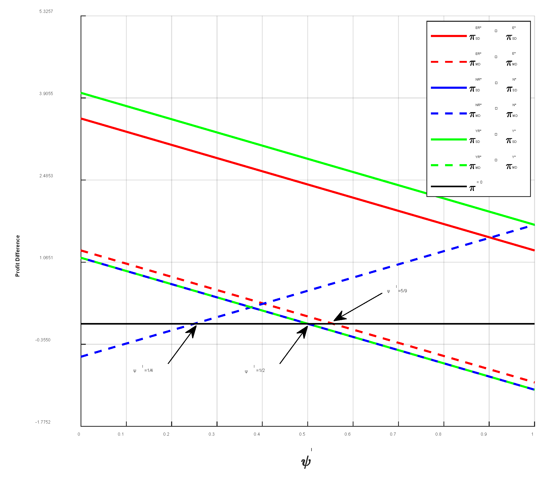
Proposition 8 demonstrates that achieving perfect supply chain coordination under blockchain requires the revenue-sharing coefficient ψ l to fall within a critical range that varies systematically with the power structure. These specific numerical intervals confirm a crucial principle: while blockchain smart contracts can automate execution and reduce traditional cooperation costs, successful coordination ultimately depends on designing contract parameters that are precisely aligned with the supply chain’s inherent power dynamics.
This finding offers managers a dual insight. First, as a technological enabler, smart contracts provide a feasible foundation for implementing complex collaborative mechanisms—such as dynamic revenue sharing—that were previously hindered by trust deficits. Second, and more importantly, technology alone is insufficient; effective coordination requires a profound understanding of the core incentives for all parties under different power structures. A dominant supplier requires a significant revenue share ( ψ N > 1 / 4 ), a leading manufacturer permits a more flexible ratio, and a balanced structure necessitates a mutually acceptable equilibrium ( ψ E < 5 / 9 ). Consequently, successful coordination hinges not only on technological implementation but also on the meticulous design of incentive structures that are tailored to the specific power context.

6. Numerical Analysis

To verify the validity and correctness of the proposed propositions and inferences, numerical simulation examples are employed. Based on market demand considerations, the relevant parameter should be greater than zero. Referring to existing research on technology investment [12,43,53], we assume b B l = 5 < b D l = 10 , g B l = 1 < g D l = 2 ,   c S l = 0.1 , c M l = 0.2 , c l = 0.15 , c S B l = 0.1 , c M B l = 0.1 , c S D l = 0.2 , c M D l = 0.2 , θ D l = 0.2 < θ B l = 0.7 . The values of all parameters are determined through calculation and presented in Table 6. Consequently, Proposition 2 and Proposition 3 are substantiated.

6.1. Key Parameters Sensitivity Analysis

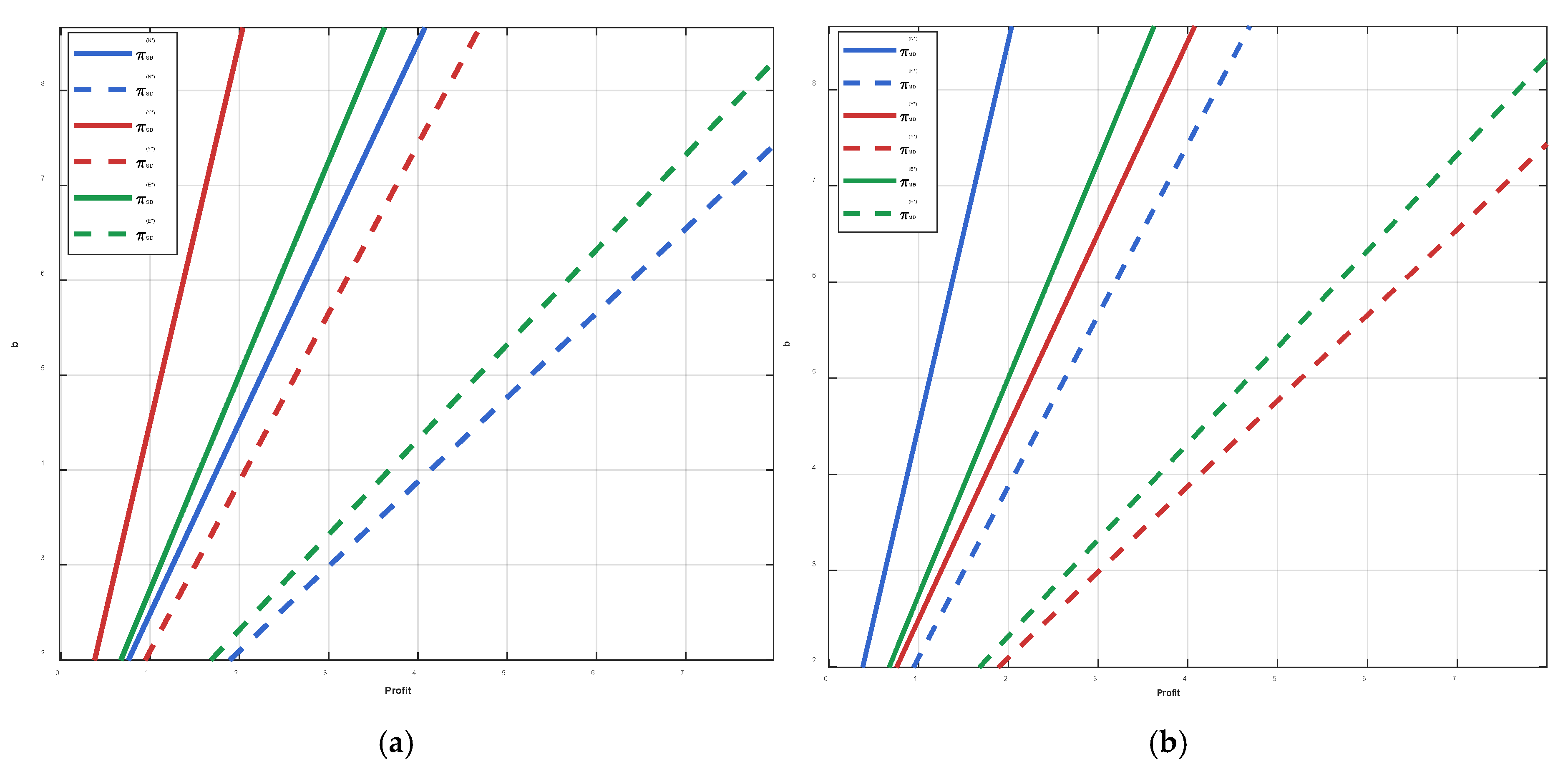
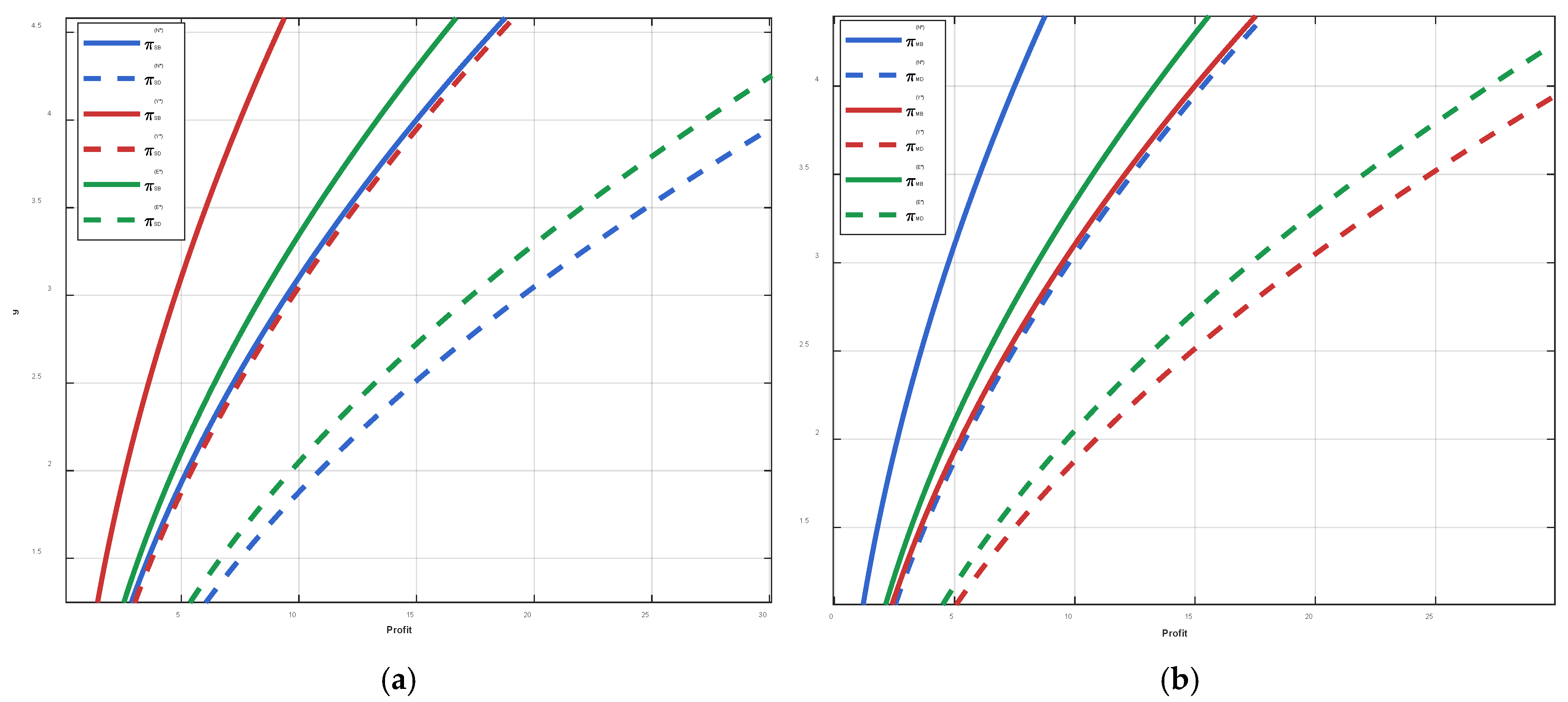
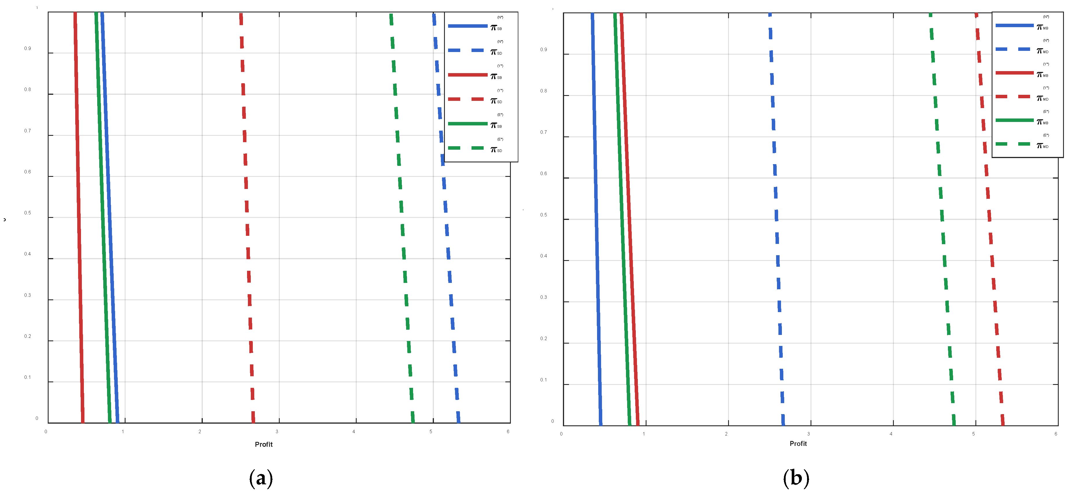
To examine the impact of key parameters on supply chain dynamics, we conducted sensitivity analyses on customer heterogeneity satisfaction ( b ), technology-induced demand gain ( g ), and the cost optimization coefficient ( θ ), as shown in Figure 2, Figure 3 and Figure 4.
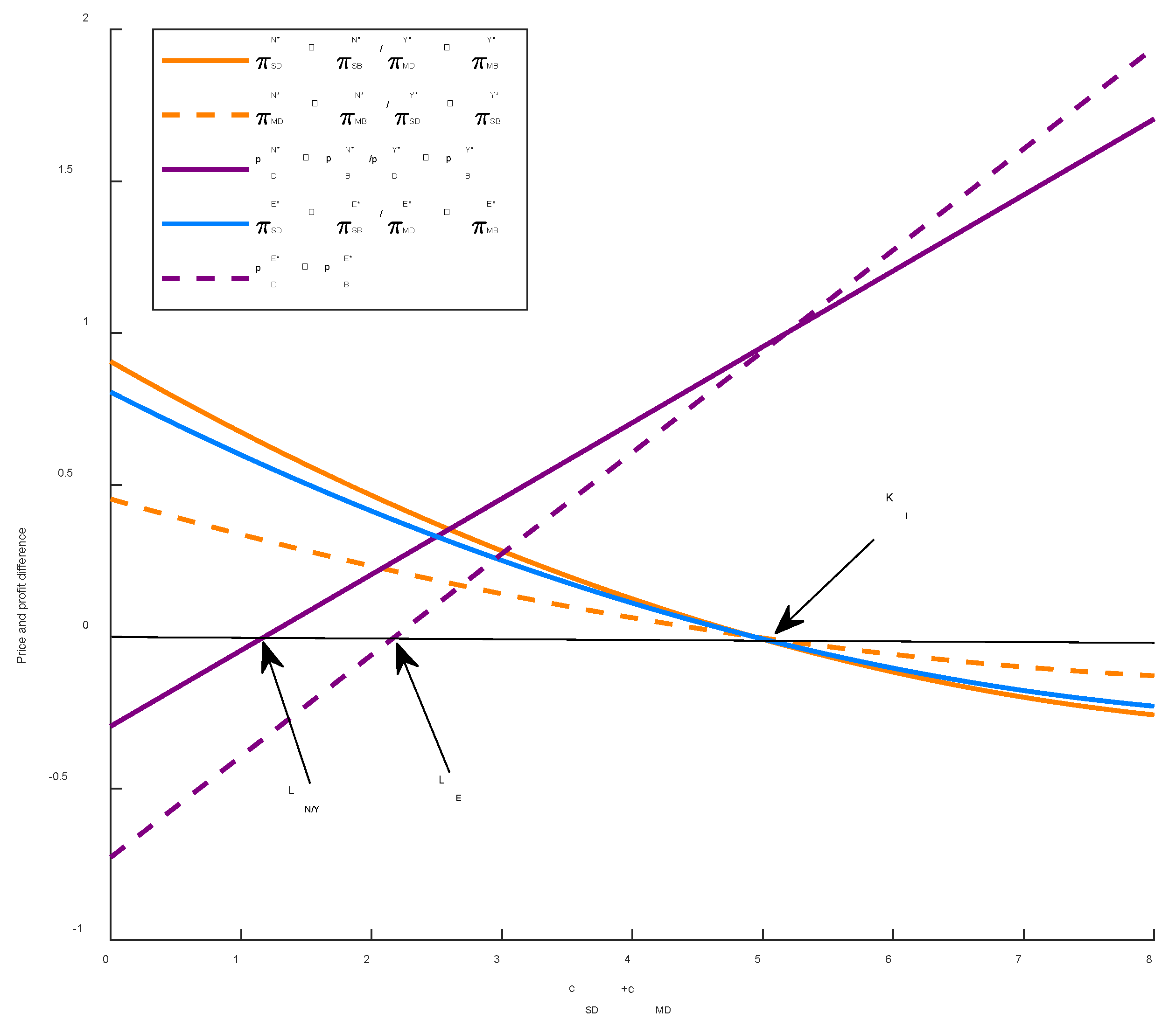
Figure 2 illustrates the interplay between customer heterogeneity satisfaction ( b ) and power structure on firm profits. As b increases—indicating a stronger corporate capability to meet diverse demands through BDBT/BDAT—the profits of both suppliers and manufacturers grow. This validates the core proposition that digital technology converts market diversity into profit by enabling precise value segmentation. Critically, the power structure acts as a value distribution lever. In the supplier-led model, the supplier’s pricing power allows it to capture incremental value most rapidly, yielding the steepest profit curve. Conversely, under manufacturer leadership, channel control enables the manufacturer to maximize its profit growth. The balanced power structure presents an intermediate state, reflecting a negotiated compromise. Across all configurations, the BDBT investment path demonstrates a superior profit trajectory, affirming its role as a strategic tool for value creation and capture in complex markets.
Figure 3 reveals the interaction between demand gain ( g ) and power structure on value creation and distribution. An increasing g value, representing the trust premium from blockchain, expands market space and creates incremental value, raising profits for all members. Again, the power structure dictates value distribution: a supplier leader leverages pricing priority to convert demand gains into profit most effectively, while a manufacturer leader uses channel control to capture value. The balanced structure, requiring benefit-sharing through negotiation, shows a moderate profit growth rate. Importantly, the BDBT path consistently outperforms other technological options, demonstrating its capacity to not only create market value through trust but also translate it into a sustainable competitive advantage, providing a clear rationale for digital transformation.
Figure 4 highlights the critical trade-off between cost optimization potential ( θ ) and its realization cost. As θ increases, the substantial investment required to achieve higher cost savings leads to a general decline in profits for all parties. While the rate of decline is similar across power structures, the vertical spacing between profit curves demonstrates the decisive role of power in setting profit baselines. At any given θ level, a firm achieves its highest profit under its own dominance, intermediate profit under balanced power, and its lowest profit when subordinate. This confirms that power establishes a pre-determined benchmark for value distribution. Notably, the BDBT investment path maintains a significantly higher profit curve across all scenarios, indicating that it not only enhances cost optimization efficiency but, more crucially, builds a defensive line against the risks of high-potential technologies by increasing the certainty of value creation, thus providing a vital risk buffer for aggressive technological upgrades.

6.2. Investment Decision-Making and Coordination Analysis

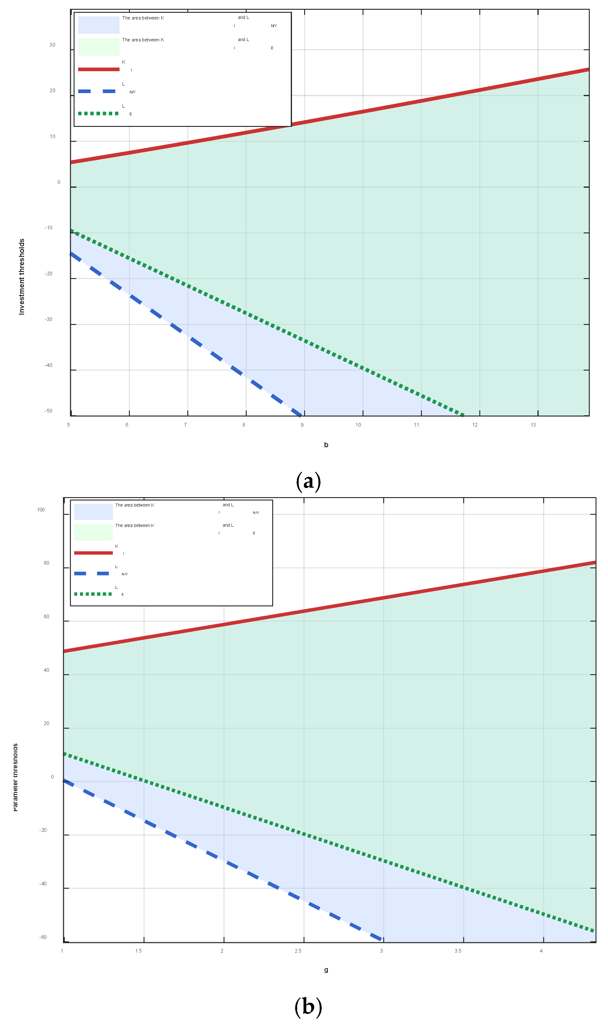
Based on the established parameter settings, we developed Figure 5, Figure 6 and Figure 7 to validate our analytical findings. Figure 5 provides intuitive verification for Propositions 4 and 5. The managerial insight it reveals is particularly significant: the investment cost threshold K l defines the absolute boundary for technological feasibility. Of greater strategic importance is the interval ( L l , K l ) , within which a “price increase and profit growth” synergy emerges in the supply chain. This phenomenon challenges conventional wisdom, as the underlying mechanism resides in the new value dimension that BDBT investment—specifically the credibility afforded by blockchain—inherently adds to the product. The market responds by accepting a price premium, while the supply chain simultaneously optimizes operational efficiency. This virtuous cycle of “value creation, market realization, and efficiency allocation” ensures that all parties achieve improved profits net of investment costs, thereby realizing Pareto coordination.
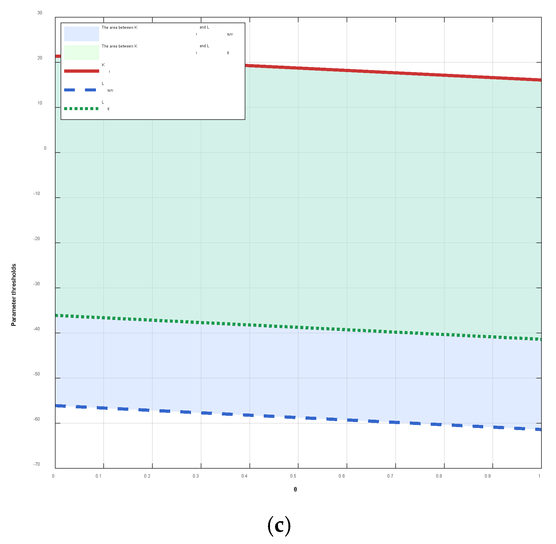
Figure 6 provides robust empirical evidence for Corollary 2 through systematic numerical simulation, visually revealing how key parameters regulate the investment threshold. This moves the study’s conclusions on investment feasibility beyond theoretical speculation. Figure 6a–c collectively demonstrate that the feasible investment region (the area below the cost threshold) is dynamically contingent on these parameters. Specifically, Figure 6a,b show that the investment threshold increases significantly with higher levels of customer heterogeneity satisfaction ( b ) and demand gain ( g ). This indicates that market diversity and the trust premium from BT substantially expand the profitable investment space, making BDBT adoption more likely for chain members. Conversely, Figure 6c reveals a critical, counterintuitive finding: an increase in the cost optimization coefficient ( θ ) lowers the investment threshold. This confirms and deepens the assertion in Corollary 2. The underlying economic logic is that pursuing extremely high cost optimization potential necessitates prohibitively high upfront investment and system complexity, which erodes project feasibility and, on a net basis, reduces the investment likelihood. In summary, these simulations transform theoretical inferences into visual decision boundaries, clearly delineating the feasible domain for BDBT investment under varying market and technical conditions.
Figure 7 illustrates the dynamic relationship between the revenue-sharing coefficient ( ψ ) and the state of supply chain coordination. The figure shows that the coordinated profit differential approaches zero only within a specific range of ψ , providing strong numerical validation for the theoretical derivation in Proposition 8. On a deeper level, the figure elucidates the design logic of the coordination contract: the effective intervals for ψ under different power structures represent equilibrium outcomes of the game among supply chain members on a blockchain-enabled credible execution platform. By strategically designing ψ , the profit distribution demands inherent to different power structures can be precisely matched, ensuring the synergistic value of BDBT investment is effectively shared to achieve ultimate supply chain coordination.

6.3. Management Insights

Based on the preceding numerical analysis and verification, this study distills several managerial implications that offer direct, actionable guidance for formulating BDBT investment and synergy strategies tailored to an enterprise’s power position.
First, this study confirms the core hypothesis that power structure dictates value distribution (H2). Consequently, before investing, firms must rigorously assess their power position within the supply chain [29,30,31]. For dominant firms (e.g., core manufacturers or large retailers), an active, offensive strategy is warranted. Similar to Walmart’s role in the IBM Food Trust initiative, the leader should proactively drive BDBT investment, leveraging its pricing and rule-making power to enhance overall supply chain value while capturing a majority share. The key decision involves weighing the high investment against the strategic control and brand premium it secures. For non-dominant firms (e.g., small and medium-sized suppliers), a collaborative defense strategy is more appropriate. Blindly complying with a leader’s investment demands can lead to profit erosion. For partners in balanced power structures, the focus should be on building co-creation and sharing mechanisms. Both parties should recognize that through Nash bargaining and coordinated contracts (e.g., cost- and revenue-sharing), they can avoid a “lose-lose” prisoner’s dilemma, achieving superior overall efficiency and a more stable partnership than under unilateral dominance.
Second, investment decisions must transition from experiential judgment to precise quantification. This study verifies the hypothesis that “Pareto improvement has a cost threshold (H1),” revealing that technological investment is only viable within specific economic boundaries [43,44]. Managers should treat the investment cost threshold K l as a rigid benchmark. By accurately calculating the operational savings ( θ ) and demand gains ( g ) created by BDBT and comparing them against the total investment cost, an investment is only feasible if the cost remains below this threshold. For instance, in the TradeLens platform co-developed by Maersk and IBM, blockchain ensures data immutability, while big data analytics optimize global shipping routes and port schedules based on this trusted information—a direct manifestation of the parameters θ and g . Furthermore, our analyses across power structures demonstrate that, under certain conditions, the BDBT technological pathway yields significantly superior performance to BDAT investment alone. This compels firms to select the BDBT pathway to construct a complete “data-to-trust” value loop.
Third, this study demonstrates that well-designed coordination contracts can effectively mitigate the distortions introduced by power asymmetries (H3). Managers should treat contract negotiation as an indispensable component of digital transformation projects [47,48]. In an imbalanced power structure, coordination contracts act as an essential buffer, protecting the weaker party and sustaining the supply chain’s long-term health. The dominant firm should recognize that strategic concessions (e.g., through revenue-sharing) can incentivize higher-quality collaboration from partners, ultimately expanding the total value pie. In a balanced power structure, the coordination contract serves as a foundational blueprint, crystallizing the willingness to cooperate into a stable operational model by clearly defining cost-sharing and profit-distribution rules.
In conclusion, in the wave of digital transformation, enterprises must avoid the trap of technological determinism. A successful BDBT strategy constitutes an organic synthesis of precise self-positioning (power analysis), astute technology selection (BDAT/BDBT), and ingenious governance design (coordination contracts). The theoretical model and decision-making framework provided by this research offer systematic guidance for navigating this complex decision-making process.

7. Conclusions

This study elucidates the decision-making mechanisms for BDBT investment within a BDAT environment by constructing a game-theoretic model contingent on power structures. The core findings demonstrate that supply chain power acts as a key regulatory mechanism for the distribution of technological value, while the identified investment cost threshold ( K l ) provides a clear benchmark for collaborative decision-making. Furthermore, the research confirms that smart contracts can achieve precise coordination across different power structures by encoding terms into automated programs, provided their parameter design aligns with the specific power configuration.
Based on these findings, we propose the following strategic recommendations: For business decision-makers, the primary step is to accurately calculate the investment thresholds ( K l and L l ) relevant to their power structure. Dominant firms should proactively assume responsibility for ecosystem development and pioneer investments when costs are controllable. Non-dominant firms must leverage contractual negotiations to ensure equitable profit distribution and cost-sharing. In collaborative design, we recommend a higher revenue-sharing coefficient ( ψ N > 1 / 4 ) for supplier-led structures and a moderate coefficient ( 0 < ψ Y < 1 / 2 ) for manufacturer-led contexts, with these terms solidified via smart contracts. Under viable conditions, all firms should prioritize the integrated BDBT pathway to maximize technological value.
For policymakers, the key to fostering BT adoption lies in building a supportive ecosystem. A primary measure is to champion universal standards for supply chain data exchange to dismantle data silos, thereby raising the industry-wide investment threshold K l by enhancing the value of technological collaboration. Secondly, establishing technology adoption funds for small and medium-sized enterprises—such as through BaaS (Blockchain-as-a-Service) platform subsidies—can reduce their investment costs ( c S D l + c M D l ) , thereby activating collaborative projects stalled by funding gaps. Additionally, regulatory “sandboxes” in critical sectors like food and pharmaceuticals could encourage the exploration of new smart contract governance models, providing templates for broader knowledge dissemination.
In summary, this study provides a theoretical foundation and a decision-making framework for supply chain members adopting BDBT, demonstrating how contractual governance can mitigate the distortion of investment incentives by power structures, thereby enabling the value leap from BDAT to BDBT.
Future research on digital technology investment should more deeply incorporate internal organizational governance structures and their interactive effects. While this paper establishes a theoretical model with parameters grounded in the literature and logical deduction, subsequent work could involve in-depth case studies or large-sample empirical analyses in specific sectors (e.g., food traceability or high-end manufacturing). Such research would help “calibrate” key parameters like θ and g more precisely, ultimately yielding more industry-specific investment decision tools.

Author Contributions

Z.L.: Formal analysis, Writing—original draft. J.H.: Resources, Writing—review and editing. Q.X.: Formal analysis, Writing—review and editing. All authors have read and agreed to the published version of the manuscript.

Funding

This work was supported by National Natural Science Foundation of China [grant numbers 71802100, 71873111].

Data Availability Statement

All simulation parameters, control equations, and source code can be provided upon request to ensure full reproducibility. No new experimental or observational data were generated during this study.

Conflicts of Interest

No potential conflict of interest was reported by the authors.

Appendix A

Appendix A.1. Proof of Proposition 1

(1)
Supplier-led
Here, the reverse induction method is used to solve the profit function. First, the derivative of the manufacturer’s profit function π M B N with respect to the selling price p B N is obtained, which gives π M B N p B N = ( ( 1 + g B N ) b B N + w B N + c M B N + θ B N c M N 2 p B N ) / b B N and 2 π M B N ( p B N ) 2 = 2 / b B N < 0 . Let π M B N p B N = 0 , and we have p B N = ( ( 1 + g B N ) b B N + w B N + c M B N + θ B N c M N ) / 2 . Substituting p B N into π S B N and taking the partial derivative with respect to w B N , then setting π S B N w B N = 0 , we can obtain w B N = ( ( 1 + g B N ) b B N + c S B N c M B N + θ B N c S N + θ B N c N θ B N c M N ) / 2 , then calculate p B N = ( 3 ( 1 + g B N ) b B N + c S B N + c M B N + θ B N c S N + θ B N c N + θ B N c M N ) / 4 and Q B N = ( ( 1 + g B N ) b B N c S B N c M B N θ B N c S N θ B N c N θ B N c M N ) / 4 b B N , Then, substituting w B N , p B N and Q B N into π S B N and π M B N , we can obtain π S B N = ( ( 1 + g B N ) b B N c S B N c M B N θ B N c S N θ B N c N θ B N c M N ) 2 / 8 b B N and π M B N = ( ( 1 + g B N ) b B N c S B N c M B N θ B N c S N θ B N c N θ B N c M N ) 2 / 16 b B N .  By the same token:
w D N = ( ( 1 + g D N ) b D N + c S D N c M D N + θ D N c S N + θ D N c N θ D N c M N ) / 2 p D N = ( 3 ( 1 + g D N ) b D N + c S D N + c M D N + θ D N c S N + θ D N c N + θ D N c M N ) / 4 Q D N = ( ( 1 + g D N ) b D N c S D N c M D N θ D N c S N θ D N c N θ D N c M N ) / 4 b D N
π S D N = ( ( 1 + g D N ) b D N c S D N c M D N θ D N c S N θ D N c N θ D N c M N ) 2 / 8 b D N π M D N = ( ( 1 + g D N ) b D N c S D N c M D N θ D N c S N θ D N c N θ D N c M N ) 2 / 16 b D N
(2)
Manufacturer-led
Let p B Y = m + w B Y , substitute it into π S B Y , and take the partial derivative with respect to w B Y , and we can obtain π S B Y w B Y = ( 1 + g B Y ) b B Y 2 w B Y + c S B Y + θ B Y c S Y + θ B Y c Y m and 2 π S B Y ( w B Y ) 2 = 2 < 0 . Let π S B Y w B Y = 0 , and we have w B Y = ( 1 + g B Y ) b B Y p B Y + c S B Y + θ B Y c S Y + θ B Y c Y . Substituting w B Y into π M B Y and taking the partial derivative with respect to p B Y , we obtain π M B Y p B Y = ( 3 ( 1 + g B Y ) b B Y + c S B Y + c M B Y + θ B Y c S Y + θ B Y c Y + θ B Y c M Y 4 p B Y ) / b B Y and 2 π M B Y ( p B Y ) 2 = 4 / b B Y < 0 . Therefore, let π M B Y p B Y = 0 , and we obtain p B Y = ( 3 ( 1 + g B Y ) b B Y + c S B Y + c M B Y + θ B Y c S Y + θ B Y c Y + θ B Y c M Y ) / 4 . Substituting p B Y into w B Y and Q B Y  gives  w B Y = ( 1 + g B Y ) b B Y + 3 c S B Y c M B Y + 3 θ B Y c S Y + 3 θ B Y c Y θ B Y c M Y / 4 and Q B Y = ( ( 1 + g B Y ) b B Y c S B Y c M B Y θ B Y c S Y θ B Y c Y θ B Y c M Y ) / 4 b B Y . Substituting p B Y , w B Y , and Q B Y into π S B Y and π M B Y , we have π S B Y = ( ( 1 + g B Y ) b B Y c S B Y c M B Y θ B Y c S Y θ B Y c Y θ B Y c M Y ) 2 / 16 b B Y and π M B Y = ( ( 1 + g B Y ) b B Y c S B Y c M B Y θ B Y c S Y θ B Y c Y θ B Y c M Y ) 2 / 8 b B Y .
By the same token:
w D Y = ( 1 + g D Y ) b D Y + 3 c S D Y c M D Y + 3 θ D Y c S Y + 3 θ D Y c Y θ D Y c M Y / 4 p D Y = ( 3 ( 1 + g D Y ) b D Y + c S D Y + c M D Y + θ D Y c S Y + θ D Y c Y + θ D Y c M Y ) / 4 Q D Y = ( ( 1 + g D Y ) b D Y c S D Y c M D Y θ D Y c S Y θ D Y c Y θ D Y c M Y ) / 4 b D Y
π S D Y = ( ( 1 + g D Y ) b D Y c S D Y c M D Y θ D Y c S Y θ D Y c Y θ D Y c M Y ) 2 / 16 b D Y π M D Y = ( ( 1 + g D Y ) b D Y c S D Y c M D Y θ D Y c S Y θ D Y c Y θ D Y c M Y ) 2 / 8 b D Y
(3)
Equilibrium of power
First, take the partial derivative of p B E in π M B E , to obtain π M B E p B E = ( ( 1 + g B E ) b B E + w B E + c M B E + θ B E c M E 2 p B E ) / b B E and 2 π M B E ( p B E ) 2 = 2 / b B E < 0 . Let π M B E p B E = 0 , and we can obtain 2 p B E = ( 1 + g B E ) b B E + w B E + c M B E + θ B E c M E (Equation (A1)). Let p B E = m + w B E , substitute it into π S B E , and then take the partial derivative of w B E to obtain  π S B E w B E = ( 1 + g B E ) b B E 2 w B E + c S B E + θ B E c S E + θ B E c E m and 2 π S B E ( w B E ) 2 = 2 < 0 .Let π S B E w B E = 0 ; then we obtain w B E = ( 1 + g B E ) b B E p B E + c S B E + θ B E c S E + θ B E c E (Equation (A2)). By solving Equations (A1) and (A2) simultaneously, the values of p B E = ( 2 ( 1 + g B E ) b B E + c S B E + c M B E + θ B E c S E + θ B E c E + θ B E c M E ) / 3 and w B E = ( ( 1 + g B E ) b B E + 2 c S B E c M B E + 2 θ B E c S E + 2 θ B E c E θ B E c M E ) / 3 can be determined. It follows that Q B E = ( ( 1 + g B E ) b B E c S B E c M B E θ B E c S E θ B E c E θ B E c M E ) / 3 b B E . Substituting p B E , w B E , and Q B E into the expressions for π S B E and π M B E yields the corresponding values for π S B E = ( ( 1 + g B E ) b B E c S B E c M B E θ B E c S E θ B E c E θ B E c M E ) 2 / 9 b B E and π M B E = ( ( 1 + g B E ) b B E c S B E c M B E θ B E c S E θ B E c E θ B E c M E ) 2 / 9 b B E .
By the same token:
w D E = ( ( 1 + g D E ) b D E + 2 c S D E c M D E + 2 θ D E c S E + 2 θ D E c E θ D E c M E ) / 3 p D E = ( 2 ( 1 + g D E ) b D E + c S D E + c M D E + θ D E c S E + θ D E c E + θ D E c M E ) / 3 Q D E = ( ( 1 + g D E ) b D E c S D E c M D E θ D E c S E θ D E c E θ D E c M E ) / 3 b D E
π S D E = ( ( 1 + g D E ) b D E c S D E c M D E θ D E c S E θ D E c E θ D E c M E ) 2 / 9 b D E π M D E = ( ( 1 + g D E ) b D E c S D E c M D E θ D E c S E θ D E c E θ D E c M E ) 2 / 9 b D E

Appendix A.2. Proof of Proposition 2

(1)
Since Q B l > 0 , it follows that ( 1 + g B l ) b B l > c S B l + c M B l + θ j l c S l + θ j l c l + θ j l c M l . For simplicity in computation, we assume that regardless of which entity dominates the supply chain, the relative magnitudes of parameters with the same meaning remain unchanged. For instance, b B N = b B Y = b B E , and we denote this common value as b B . Based on this assumption, it can be calculated that w B N w B Y = ( ( 1 + g B ) b B c S B c M B θ B c S θ B c θ B c M ) / 4 > 0 , which implies w B N > w B Y Similarly, since w B E w B Y = ( ( 1 + g B ) b B c S B c M B θ B c S θ B c θ B c M ) / 12 > 0 , we have w B E > w B Y . Furthermore, given that w B N w B E = ( ( 1 + g B ) b B c S B c M B θ B c S θ B c θ B c M ) / 6 > 0 , it follows that w B N > w B E . In summary, we can conclude that w B N > w B E > w B Y
By the same token: w D N > w D E > w D Y .
(2)
Since p B N p B Y = 0 , it follows that p B N = p B Y Furthermore, given that p B Y p B E = ( 1 + g B ) b B c S B c M B θ B c S θ B c θ B c M / 12 and ( 1 + g B ) b B > c S B + c M B + θ B c S + θ B c + θ B c M , we can deduce that p B Y p B E > 0 , which implies p B Y > p B E , In conclusion, p B N = p B Y > p B E , can be established.
By the same token, p D N = p D Y > p D E .

Appendix A.3. Proof of Proposition 3

From the formula structure of π S j N , π S j Y , π S j E and π M j N , π M j Y , π M j E , it is obvious that: π S j N > π S j E > π S j Y , π M j Y > π M j E > π M j N .

Appendix A.4. Proof of Corollary 1

(3)
In a supplier-led supply chain, given that π S B N b B N = ( ( 1 + g B N ) b B N c S B N c M B N θ B N c S N θ B N c N θ B N c M N ) ( ( 1 + g B N ) b B N + c S B N + c M B N + θ B N c S N + θ B N c N + θ B N c M N ) / 8 b B N 2 , and both ( 1 + g B N ) b B N c S B N c M B N θ B N c S N θ B N c N θ B N c M N > 0 and ( 1 + g B N ) b B N + c S B N + c M B N + θ B N c S N + θ B N c N + θ B N c M N > 0 , it follows that π S B N b B N > 0 . Similarly, π M B N b B N > 0 can be derived. For the manufacturer-led supply chain and the supply chain under equilibrium conditions, through an analogous calculation process, it can be shown that π S j l b j l > 0 and π M j l b j l > 0 , where j B , D , l { Y , E } . Similarly, π S j l g j l > 0   a n d   π M j l g j l > 0 , where j B , D , l { N , Y , E } .
Since π S B N θ B N = ( ( 1 + g B N ) b B N c S B N c M B N θ B N c S N θ B N c N θ B N c M N ) ( c S N + c N + c M N ) / 4 b B N and ( 1 + g B N ) b B N c S B N c M B N θ B N c S N θ B N c N θ B N c M N > 0 and c S N + c N + c M N < 0 , it follows that π S B N θ B N < 0 . Similarly, π M B N θ B N < 0 can also be derived. For both the manufacturer-led supply chain and the supply chain under equilibrium conditions, a comparable calculation process yields π S j l θ j l < 0 and π M j l θ j l < 0 , where j B , D , l { Y , E } .

Appendix A.5. Proof of Proposition 4

Under the supplier’s dominance, since π S D N π S B N = ( 1 + g D N ) b D N c S D N c M D N θ D N c S N θ D N c N θ D N c M N 2 8 b D N ( 1 + g B N ) b B N c S B N c M B N θ B N c S N θ B N c N θ B N c M N 2 8 b B N and ( 1 + g j N ) b j N c S j N c M j N θ j N c S N θ j N c N θ j N c M N > 0 , it can be obtained that when c S D N + c M D N < b D N / b B N ( c S B N + c M B N ) + b D N ( ( 1 + g D N ) b D N ( 1 + g B N ) b B N ) + G 1 ( b D N / b B N θ B N θ D N ) , π S D N > π S B N , where G 1 = c S N + c N + c M N .
Let G 1 = c S N + c N + c M N = c S E + c E + c M E = c S Y + c Y + c M Y . By the same token, it can be proved that:
When c S D Y + c M D Y < b D Y / b B Y ( c S B Y + c M B Y ) + b D Y ( ( 1 + g D Y ) b D Y ( 1 + g B Y ) b B Y ) + G 1 ( b D Y / b B Y θ B Y θ D Y ) , there is π S D Y > π S B Y .
When c S D E + c M D E < b D E / b B E ( c S B E + c M B E ) + b D E ( ( 1 + g D E ) b D E ( 1 + g B E ) b B E ) + G 1 ( b D E / b B E θ B E θ D E ) , there is π S D E > π S B E .
For manufacturers, the same method can be applied to demonstrate that when c S D N + c M D N < b D N / b B N ( c S B N + c M B N ) + b D N ( ( 1 + g D N ) b D N ( 1 + g B N ) b B N ) + G 1 ( b D N / b B N θ B N θ D N ) , then π M D N > π M B N . Similarly, when c S D Y + c M D Y < b D Y / b B Y ( c S B Y + c M B Y ) + b D Y ( ( 1 + g D Y ) b D Y ( 1 + g B Y ) b B Y ) + G 1 ( b D Y / b B Y θ B Y θ D Y ) , it follows that π M D Y > π M B Y ; and when c S D E + c M D E < b D E / b B E ( c S B E + c M B E ) + b D E ( ( 1 + g D E ) b D E ( 1 + g B E ) b B E ) + G 1 ( b D E / b B E θ B E θ D E ) , π M D E > π M B E .
In summary, when c S D l + c M D l < K l , we obtain π S D l > π S B l , π M D l > π M B l , w h e r e K l | l { N , Y , E } = b D l / b B l ( c S B l + c M B l ) + b D l ( ( 1 + g D l ) b D l ( 1 + g B l ) b B l ) + G 1 ( b D l / b B l θ B l θ D l ) . Therefore, the proposition is proven.

Appendix A.6. Proof of Proposition 5

Firstly, for computational convenience, we denote G 1 = c S N + c N + c M N = c S E + c E + c M E = c S Y + c Y + c M Y . Through Proposition 1, we have p D N p B N = ( 3 ( ( 1 + g D N ) b D N ( 1 + g B N ) b B N ) + c S D N + c M D N c S B N c M B N + G 1 θ D N θ B N ) / 4. Therefore, it can be concluded that when c S D N + c M D N > L N , p D N > p B N , where L N = c S B N + c M B N 3 ( ( 1 + g D N ) b D N ( 1 + g B N ) b B N ) G 1 θ D N θ B N . From Proposition 4, it can be obtained that when c S D N + c M D N < K N , there is π S D N > π S B N , π M D N > π M B N . In conclusion, when L N < c S D N + c M D N < K N , there is p D N > p B N and π S D N > π S B N , π M D N > π M B N .
By the same token, Similarly, when c S D Y + c M D Y > L Y , we have p D Y > p B Y , where L Y = c S B Y + c M B Y G 1 θ D Y θ B Y 3 ( ( 1 + g D Y ) b D Y ( 1 + g B Y ) b B Y ) . Furthermore, according to Proposition 4, if L Y < c S D Y + c M D Y < K Y , then p D Y > p B Y , π S D Y > π S B Y and π M D Y > π M B Y . When c S D E + c M D E > L E , we have p D E > p B E , where L E = c S B E + c M B E G 1 θ D E θ B E 2 ( ( 1 + g D E ) b D E ( 1 + g B E ) b B E ) . According to Proposition 4, it follows that when L E < c S D E + c M D E < K E , we have p D E > p B E , π S D E > π S B E a n d π M D E > π M B E .
To sum up, let L l = { L N , L Y , L E } , when L l < c S D l + c M D l < K l , we have p D l > p B l , π S D l > π S B l a n d π M D l > π M B l . The proposition is proved.

Appendix A.7. Proof of Proposition 6

From π C l p D l = ( ( 1 + g D C l ) b D C l + c S D C l + c M D C l + θ D C l G 1 2 p D C l ) / b D C l and 2 π C l ( p D C l ) 2 = 2 / b D C l < 0 . Let π C l p D C l = 0 , which leads to p D C l = ( ( 1 + g D C l ) b D C l + c S D C l + c M D C l + θ D C l G 1 ) / 2 . Given that Q D C l = 1 p D C l / b D C l , it follows that Q D C l = ( ( 1 + g D C l ) b D C l c S D C l c M D C l θ D C l G 1 ) / 2 b D C l . Substituting p D C l and Q D C l into π C results in π C l = ( ( 1 + g D C l ) b D C l c S D C l c M D C l θ D C l G 1 ) 2 / 4 b D C l .

Appendix A.8. Proof of Proposition 7

(1)
For supplier-led supply chains:
First, take the derivative of the manufacturer’s profit function π M D N R with respect to the selling price p D N , and we obtain π M D N R p D N = ( ψ N ( 1 + g D N ) b D N + w D N + c M D N + θ D N c M N + ( 1 χ N ) c S D N 2 ψ N p D N ) / b D N and 2 π M B N R ( p D N ) 2 = 2 ψ N / b D N < 0 . Then let π M B N R p D N = 0 , and we can obtain p D N ( w D N ) = ( ψ N ( 1 + g D N ) b D N + w D N + ( 1 χ N ) c S D N + c M D N + θ D N c M N ) / 2 ψ N . Then let p D N w D N = p D C N , and we can obtain w D N = ( χ N + ψ N 1 ) c S D N + ( ψ N 1 ) c M D N + θ D N ψ N ( c S N + c N ) + ( ψ N 1 ) θ D N c M N . Substituting w D N and p D N into π M D N R and π S D N R gives π S D N R = ( 1 ψ N ) ( ( 1 + g D N ) b D N Ρ 1 ) 2 / 4 b D N and π M D N R = ψ N ( ( 1 + g D N ) b D N Ρ 1 ) 2 / 4 b D N , where Ρ 1 = c M D N + c S D N + θ D N c S N + θ D N c N + θ D N c M N .
(2)
For manufacturer-led supply chains:
Let p D Y = m + w D Y , substitute it into π S D Y R , and take the partial derivative with respect to w D Y . We can obtain π S D Y R w D Y = ( 2 ψ Y ( 1 + g D Y ) b D Y w D Y + c S D Y + θ D Y c S Y + θ D Y c Y + χ Y c M D Y ( 3 2 ψ Y ) ( m + w D Y ) ) / b D Y = ( 2 ψ Y ( 1 + g D Y ) b D Y w D Y + c S D Y + θ D Y c S Y + θ D Y c Y + χ Y c M D Y ( 3 2 ψ Y ) p D Y ) / b D Y , and 2 π S B Y ( w B Y ) 2 < 0 . Then let π S D l R w D Y = 0 , and we can obtain w D Y ( p D Y ) = 2 ψ Y ( 1 + g D Y ) b D Y + c S D Y + θ D Y c S Y + θ D Y c Y + χ Y c M D Y ( 3 2 ψ Y ) p D Y . Substituting p D C Y = ( ( 1 + g D Y ) b D Y + c S D Y + c M D Y + θ D Y c S Y + θ D Y c Y + θ D Y c M Y ) / 2 into w D Y gives w D Y = ( ( 1 + g D Y ) b D Y + 2 ψ Y 1 c S D Y + 2 χ Y 3 + 2 ψ Y c M D Y + 2 ψ Y θ D Y θ D Y c Y + c S Y 3 2 ψ Y θ D Y c M Y ) / 2 . Then, substituting p D Y and w D Y into π S D Y R and π M D Y R for calculation, we can obtain π S D Y R = 2 ψ Y ( ( 1 + g D Y ) b D Y Ρ 2 ) 2 / 4 b D Y and π M D Y R = 1 ψ Y ( ( 1 + g D Y ) b D Y Ρ 2 ) 2 / 4 b D Y , where Ρ 2 = c M D Y + c S D Y + θ D Y c S Y + θ D Y c Y + θ D Y c M Y .
(3)
For a two-level supply chain with balanced rights:
Since both the manufacturer and the supplier aim to maximize their respective profits, the manufacturer’s optimal selling price is set as p D E = p D C E = ( 1 + g D E ) b D E + c S D E + c M D E + θ D E G 1 2 . For the optimal wholesale price of the supplier, let p D E = m + w D E , substitute it into π S D E , and then take the partial derivative with respect to w D E . We can obtain π S D E w D E = ( 2 ψ E ( 1 + g D E ) b D E w D E + θ D E c S E + θ D E c E + χ E ( c M D E + c S D E ) ( 3 2 ψ E ) ( m + w D E ) ) / b D E = ( 2 ψ E ( 1 + g D E ) b D E w D E + θ D E c S E + θ D E c E + χ E ( c M D E + c S D E ) ( 3 2 ψ E ) p D E ) / b D E and 2 π S D E ( w D E ) 2 < 0 . Then let π S D E w D E = 0 , and we can obtain w D E ( p D E ) = 2 ψ E ( 1 + g D E ) b D E + θ D E c S E + θ D E c E + χ E ( c M D E + c S D E ) ( 3 2 ψ E ) p D E . Substituting p D E , we obtain w D E = ( ( 1 + g D E ) b D E + 2 χ E 3 + 2 ψ E ( c M D E + c S D E ) + 2 ψ E θ D E θ D E c E + c S E 3 2 ψ E θ D E c M E ) / 2 . Finally, substituting p D E and w D E into π S D E R and π M D E R gives π S D E R = 2 ψ E ( ( 1 + g D E ) b D E Ρ 3 ) 2 / 4 b D E and π M D E R = 1 ψ E ( ( 1 + g D E ) b D E Ρ 3 ) 2 / 4 b D E , where Ρ 3 = c M D E + c S D E + θ D E c S E + θ D E c E + θ D E c M E .

Appendix A.9. Proof of Proposition 8

(1)
Supplier-led
Let π S D N R π S D N > 0 , n ψ N < 3 / 4 , it satisfies π S D N R > π S D N . Let π M D N R π M D N > 0 , when 1 / 4 < ψ N , it satisfies π M D N R > π M D N . Therefore, when 1 / 4 < ψ N < 1 / 2 , there is π S D N R > π S D N and π M D N R > π M D N .
(2)
Manufacturer-led
Let π S D Y R π S D Y > 0 , when ψ Y < 3 / 4 , it satisfies π S D Y R > π S D Y . Let π M D Y R π M D Y > 0 , when ψ Y < 1 / 2 , it satisfies π M D Y R > π M D Y . Therefore, when 0 < ψ Y < 1 / 2 , there is π S D Y R > π S D Y and π M D Y R > π M D Y .
(3)
Balanced Mode
Let π S D E R π S D E > 0 and 0 < ψ E < 1 ; thus, the inequality π S D E R > π S D E always holds. Suppose π M D E R π M D E > 0 , it can then be derived that π M D E R > π M D E is satisfied when ψ Y < 5 / 9 . Consequently, when 0 < ψ E < 5 / 9 , both π S D E R > π S D E and π M D E R > π M D E  are valid.

References

  1. Park, K.O. A study on sustainable usage intention of blockchain in the big data era: Logistics and supply chain management companies. Sustainability 2020, 12, 10670. [Google Scholar] [CrossRef]
  2. Jabbar, A.; Akhtar, P.; Ali, S.I. The interplay between blockchain and big data analytics for enhancing supply chain value creation in micro, small, and medium enterprises. Ann. Oper. Res. 2025, 350, 649–671. [Google Scholar]
  3. Ren, S.; Choi, T.M.; Lee, K.M.; Lin, L. Intelligent service capacity allocation for cross-border e-commerce related third-party forwarding logistics operations: A deep learning approach. Transp. Res. Part E Logist. Transp. Rev. 2020, 134, 101834. [Google Scholar] [CrossRef]
  4. Medina, M.J.; Baudet, C.; Lebraty, J.F. Blockchain and agency theory in supply chain management: A question of trust. Int. J. Inf. Manag. 2024, 75, 102747. [Google Scholar] [CrossRef]
  5. Sina. Blockchain Integration into Medical Scenarios: Achieving “Multi-Party Trust” Through Smart Contracts. Available online: https://news.sina.com.cn/o/2024-10-20/doc-inctfent2617686.shtml (accessed on 20 October 2024).
  6. Walmart. Blockchain + Supply Chain! Walmart is Piloting Food Traceability. Available online: https://www.walmart.cn/assist-two/1030.html (accessed on 18 June 2025).
  7. Hader, M.; Tchoffa, D.; El Mhamedi, A.; Ghodous, P.; Dolgui, A.; Abouabdellah, A. Applying integrated blockchain and big data technologies to improve supply chain traceability and information sharing in the textile sector. J. Ind. Inf. Integr. 2022, 28, 100345. [Google Scholar] [CrossRef]
  8. Yadav, S.; Singh, S.P. Blockchain critical success factors for sustainable supply chain. Resour. Conserv. Recycl. 2020, 152, 104505. [Google Scholar] [CrossRef]
  9. Wang, H.; Wang, C.; Li, M.; Xie, Y. Blockchain technology investment strategy for shipping companies under competition. Ocean Coast. Manag. 2023, 243, 106696. [Google Scholar] [CrossRef]
  10. Chen, W.; Cui, M.; Quayson, M.; Du, H. Price and carbon emission reduction technology competition in the electricity supply chain based on power structure. RAIRO-Oper. Res. 2024, 58, 4621–4650. [Google Scholar] [CrossRef]
  11. Shan, R.; Luo, L.; Xiang, B. Optimal pricing strategies with remanufacturing technological innovation under different power structures. INFOR Inf. Syst. Oper. Res. 2022, 60, 201–243. [Google Scholar] [CrossRef]
  12. Xu, L.; Gao, R.; Xie, Y.; Du, P. To be or not to be? Big data business investment decision-making in the supply chain. Sustainability 2019, 11, 2298. [Google Scholar] [CrossRef]
  13. Li, Q.; Ma, M.; Shi, T.; Zhu, C. Green investment in a sustainable supply chain: The role of blockchain and fairness. Transp. Res. Part E Logist. Transp. Rev. 2022, 167, 102908. [Google Scholar] [CrossRef]
  14. Dai, Y.; Zhang, Y.; Song, H.; Zhou, L.; Li, H. Investment decision-making of closed-loop supply chain driven by big data technology. J. Ind. Manag. Optim. 2023, 19, 4123–4140. [Google Scholar] [CrossRef]
  15. Zheng, Y.; Xu, Y.; Qiu, Z. Blockchain traceability adoption in agricultural supply chain coordination: An evolutionary game analysis. Agriculture 2023, 13, 184. [Google Scholar] [CrossRef]
  16. Gaski, J.F.; Nevin, J.R. The differential effects of exercised and unexercised power sources in a marketing channel. J. Mark. Res. 1985, 22, 130–142. [Google Scholar] [CrossRef]
  17. Kim, J.S.; Kwak, T.C. Game theoretic analysis of the bargaining process over a long-term replenishment contract. J. Oper. Res. Soc. 2007, 58, 769–778. [Google Scholar] [CrossRef]
  18. Luo, Z.; Chen, X.; Kai, M. The effect of customer value and power structure on retail supply chain product choice and pricing decisions. Omega 2018, 77, 115–126. [Google Scholar] [CrossRef]
  19. Wan, N.; Fan, J.; Chen, W. Platform coupon promotion and its effect on an O2O retail supply chain under different power structures. Electron. Commer. Res. 2025. [Google Scholar] [CrossRef]
  20. Choi, S.C. Price competition in a channel structure with a common retailer. Mark. Sci. 1991, 10, 271–296. [Google Scholar] [CrossRef]
  21. Wang, W.B.; Sun, Q.; Yan, X.X.; Liu, Y.Q. Dual-channel supply chain financing operation strategy considering free-riding effect under different power structures. Sustainability 2022, 14, 9379. [Google Scholar] [CrossRef]
  22. Tatarczak, A.; Gola, A. An integrated fuzzy multi-criteria approach for partner selection in horizontal cooperation. Arch. Transp. 2025, 74, 23–42. [Google Scholar] [CrossRef]
  23. Li, M.; Mizuno, S. Dynamic pricing and inventory management of a dual-channel supply chain under different power structures. Eur. J. Oper. Res. 2022, 303, 273–285. [Google Scholar] [CrossRef]
  24. Jin, L.; Zheng, B.; Huang, S. Pricing and coordination in a reverse supply chain with online and offline recycling channels: A power perspective. J. Clean. Prod. 2021, 298, 126786. [Google Scholar] [CrossRef]
  25. Shi, R.; Zhao, L.; Guo, C.; Gu, X. A consensus decision-making model considering empathetic preferences and power structure of the poverty alleviation e-commerce supply chain. Complexity 2022, 2022, 2801930. [Google Scholar] [CrossRef]
  26. Li, Z.; Xu, Y.; Deng, F.; Liang, X. Impacts of power structure on sustainable supply chain management. Sustainability 2017, 10, 55. [Google Scholar] [CrossRef]
  27. Lai, L.; Liu, J.; Yang, J. Farmer-supermarket direct purchase model: Considering power asymmetry. Manag. Decis. 2025. [Google Scholar] [CrossRef]
  28. Gao, A.; Liu, B.; Yue, S. The impact of channel power structures on integrated mode of recycling in a closed-loop battery supply chain. Comput. Ind. Eng. 2025, 208, 111378. [Google Scholar] [CrossRef]
  29. Yuan, M.; Qiu, R.; Sun, M.; Shao, S.; Fan, Z.P.; Xu, H. Blockchain implementation decisions in a dual-channel supply chain under different market power structures. Int. J. Prod. Res. 2025, 63, 5238–5262. [Google Scholar] [CrossRef]
  30. Xia, L.; Wang, L.; Xiao, R.; Wang, J.; Hou, P. Blockchain and pricing strategies in supply chains considering consumer traceability preference and power structure. Int. J. Prod. Res. 2025. [Google Scholar] [CrossRef]
  31. Xu, X.; Chen, J.; Liu, S.; Yu, Y.; Cheng, T.C. Should a manufacturer adopt blockchain when its competitor discloses blockchain-enabled product quality information? Int. J. Prod. Res. 2025, 63, 5217–5237. [Google Scholar] [CrossRef]
  32. Vazquez Melendez, E.I.; Bergey, P.; Smith, B. Blockchain technology for supply chain provenance: Increasing supply chain efficiency and consumer trust. Supply Chain Manag. Int. J. 2024, 29, 706–730. [Google Scholar] [CrossRef]
  33. Pattanayak, S.; Ramkumar, M.; Goswami, M.; Rana, N.P. Blockchain technology and supply chain performance: The role of trust and relational capabilities. Int. J. Prod. Econ. 2024, 271, 109198. [Google Scholar] [CrossRef]
  34. Shamsuzzoha, A.; Shahzad, K.; Nousiainen, E.; Ranta, M.; Helo, P.; Govindan, K. Ensuring supply chain transparency by deploying blockchain-enabled technology: An overview with demonstration. Int. J. Intell. Syst. 2025, 2025, 7304193. [Google Scholar] [CrossRef]
  35. Sri Vigna Hema, V.; Manickavasagan, A. Blockchain implementation for food safety in supply chain: A review. Compr. Rev. Food Sci. Food Saf. 2024, 23, e70002. [Google Scholar] [CrossRef]
  36. Guo, W.; Yao, K. Supply chain governance of agricultural products under big data platform based on blockchain technology. Sci. Program. 2022, 2022, 4456150. [Google Scholar] [CrossRef]
  37. Dong, C.; Huang, Q.; Fang, D. Channel selection and pricing strategy with supply chain finance and blockchain. Int. J. Prod. Econ. 2023, 265, 109006. [Google Scholar] [CrossRef]
  38. Qin, J.; Fu, H.; Wang, Z.; Lyu, X. Financing decisions in capital-constrained supply chains considering uncertain emission reduction outputs and blockchain technology applications. Int. J. Prod. Res. 2025. [Google Scholar] [CrossRef]
  39. Wong, S.; Yeung, J.K.W.; Lau, Y.Y.; So, J. Technical sustainability of cloud-based blockchain integrated with machine learning for supply chain management. Sustainability 2021, 13, 8270. [Google Scholar] [CrossRef]
  40. Alwi, A.; Sasongko, N.A.; Suryana, Y.; Subagyo, H. Blockchain and big data integration design for traceability and carbon footprint management in the fishery supply chain. Egypt. Inform. J. 2024, 26, 100481. [Google Scholar] [CrossRef]
  41. Sundarakani, B.; Ajaykumar, A.; Gunasekaran, A. Big data driven supply chain design and applications for blockchain: An action research using case study approach. Omega 2021, 102, 102452. [Google Scholar] [CrossRef]
  42. Ullah, A.; Zhang, Q.; Treiblmaier, H.; Ahmad, S. Blockchain and big data-optimized supply chains as facilitators of eco-innovative firm performance. Sustain. Futures 2025, 10, 101311. [Google Scholar] [CrossRef]
  43. Liu, P.; Long, Y.; Song, H.C.; He, Y.D. Investment decision and coordination of green agri-food supply chain considering information service based on blockchain and big data. J. Clean. Prod. 2020, 277, 123646. [Google Scholar] [CrossRef]
  44. Liu, P.; Zhang, Z.; Dong, F.Y. Subsidy and pricing strategies of an agri-food supply chain considering the application of big data and blockchain. RAIRO-Oper. Res. 2022, 56, 1995–2014. [Google Scholar] [CrossRef]
  45. Li, L.; Chai, Q.; Lin, J.; Luo, X. Examining the interplay between blockchain capability and big data analytics capability in driving sustainable product innovation: A mixed-methods approach. Bus. Strategy Environ. 2025. [Google Scholar] [CrossRef]
  46. Dey, S.K.; Kundu, K.; Das, P. Digital technology based game-theoretic pricing strategies in a three-tier perishable food supply chain. Ann. Oper. Res. 2024. [Google Scholar] [CrossRef]
  47. Ran, W.; Wang, Y.; Yang, L.; Liu, S. Coordination mechanism of supply chain considering the bullwhip effect under digital technologies. Math. Probl. Eng. 2020, 2020, 3217927. [Google Scholar] [CrossRef]
  48. Dou, G.; Wei, K.; Sun, T.; Ma, L. Blockchain technology adoption in a supply chain: Channel leaderships and environmental implications. Transp. Res. Part E Logist. Transp. Rev. 2024, 192, 103788. [Google Scholar] [CrossRef]
  49. Xu, X.; Liu, M.; Wang, X.; Chen, H.; Kang, C. Investment strategy for blockchain technology in a shipping supply chain. Ocean Coast. Manag. 2022, 226, 106263. [Google Scholar] [CrossRef]
  50. Li, Y.; Tan, C.; Ip, W.H.; Wu, C.H. Dynamic blockchain adoption for freshness-keeping in the fresh agricultural product supply chain. Expert Syst. Appl. 2023, 217, 119494. [Google Scholar] [CrossRef]
  51. Wu, C.; Xu, C.; Zhao, Q.; Zhu, J. Research on financing strategy under the integration of green supply chain and blockchain technology. Comput. Ind. Eng. 2023, 184, 109598. [Google Scholar] [CrossRef]
  52. Yang, T.; Ma, C.; Mi, X. The transformative potential of blockchain technology in developing green supply chain: An evolutionary perspective on complex networks. Comput. Ind. Eng. 2024, 197, 110548. [Google Scholar] [CrossRef]
  53. Liu, P.; Yi, S.P. A study on supply chain investment decision-making and coordination in the big data environment. Ann. Oper. Res. 2018, 270, 235–253. [Google Scholar] [CrossRef]
  54. Zhang, Y.; Kou, H. Bank financing or e-commerce platform financing: Green supply chain financing strategies with blockchain integration. Expert Syst. Appl. 2026, 299, 129912. [Google Scholar] [CrossRef]
  55. Petruzzi, N.C.; Dada, M. Pricing and the newsvendor problem: A review with extensions. Oper. Res. 1999, 47, 183–194. [Google Scholar] [CrossRef]
  56. Pan, X.; Pan, X.; Song, M.; Ai, B.; Ming, Y. Blockchain technology and enterprise operational capabilities: An empirical test. Int. J. Inf. Manag. 2020, 52, 101946. [Google Scholar] [CrossRef]
  57. Guan, Z.; Ye, T.; Yin, R. Channel coordination under Nash bargaining fairness concerns in differential games of goodwill accumulation. Eur. J. Oper. Res. 2020, 285, 916–930. [Google Scholar] [CrossRef]
  58. Fan, J.; Ni, D.; Fang, X. Liability cost sharing, product quality choice, and coordination in two-echelon supply chains. Eur. J. Oper. Res. 2020, 284, 514–537. [Google Scholar] [CrossRef]
  59. Zissis, D.; Ioannou, G.; Burnetas, A. Coordinating lot sizing decisions under bilateral information asymmetry. Prod. Oper. Manag. 2020, 29, 371–387. [Google Scholar] [CrossRef]
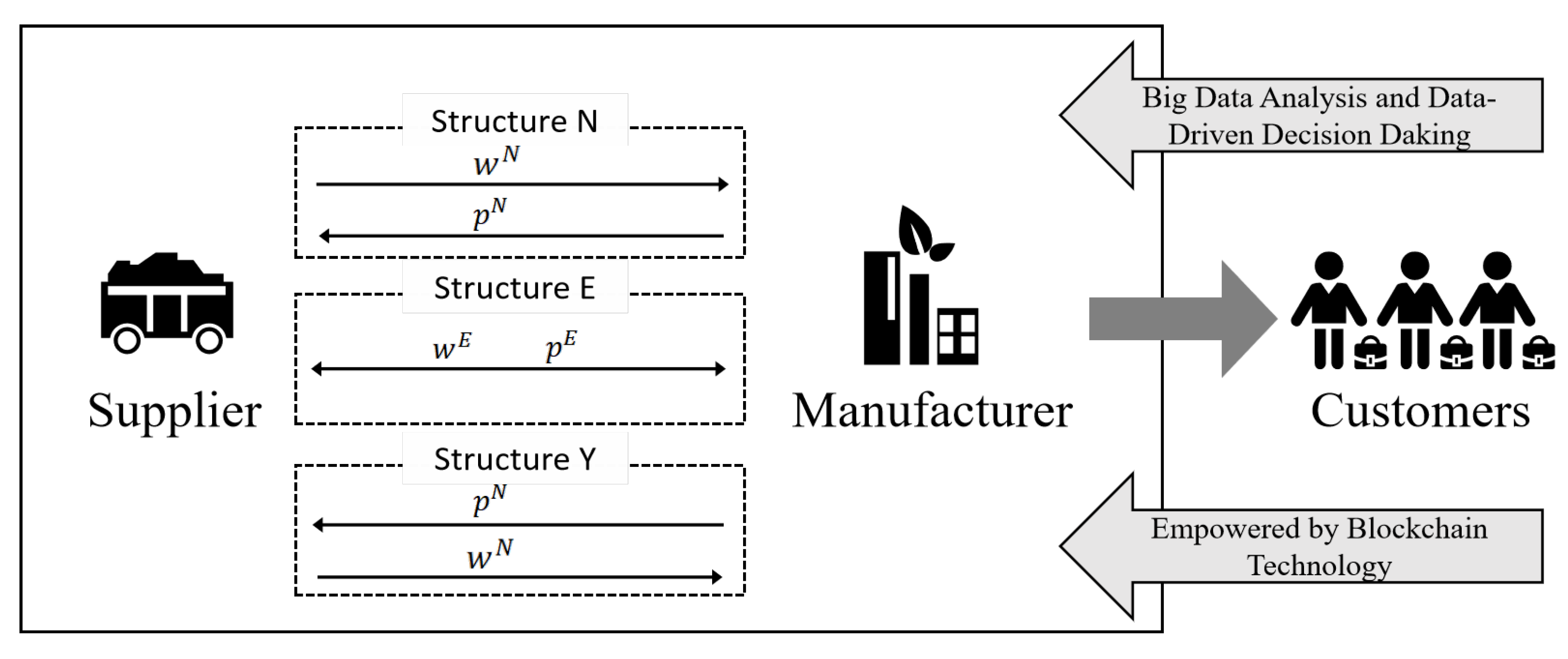
Figure 1. Schematic diagram of BT investment in the supply chain driven by BDAT.
Systems 13 01029 g001
Figure 2. (a) The impact of b  on suppliers’ profits under different power structures (left). (b) The impact of b on manufacturers’ profits under different power structures (right).
Systems 13 01029 g002
Figure 3. (a) The impact of g on supplier profits under different power structures (left). (b) The impact of g on manufacturers’ profits under different power structures (right).
Systems 13 01029 g003
Figure 4. (a) The impact of θ on supplier profits under different power structures (left). (b) The impact of θ on manufacturers’ profits under different power structures (right).
Systems 13 01029 g004
Figure 5. Supply Chain Investment Conditions in BDBT Under Various Power Structures.
Systems 13 01029 g005
Figure 6. (a) The influence of parameter b on the investment threshold. (b) The influence of parameter g on the investment threshold. (c) The influence of parameter θ on the investment threshold.
Systems 13 01029 g006aSystems 13 01029 g006b
Figure 7. Supply Chain Coordination Conditions Under Various Power Structures.
Systems 13 01029 g007
Table 1. Comparative Analysis of Research Literature.
AuthorResearch ObjectiveResearch MethodologyPower StructuresBDATBT
Xu et al. [12]Assessing the impact of big data investment on supply chain sustainability and coordination.Stackelberg GameSupplier-Led
Liu et al. [43]Investigating decision-making and coordination mechanisms for ISBD (big data-based information services) investments in green agricultural supply chains.Stackelberg GameProducer-Led
Xu et al. [49]An analysis of BT investment strategies within the shipping supply chain in the post-pandemic era.Stackelberg GamePort-Led
Li et al. [13]Exploring the impact of retailers’ emotional equity concerns on manufacturer blockchain adoption and supply chain performance.Game theory analysisRetailer’s decisions are influenced by the manufacturer
Li et al. [50]An analysis of the application effectiveness of blockchain technology in the supply chain management of fresh agricultural products.Dynamic Optimization GameRetailer-Led
Liu et al. [44]Research on Subsidy and Pricing Strategies in the Agricultural Product Supply Chain in the Context of Big Data and Blockchain TechnologyStackelberg GameProducer-Led
Wu et al. [51]Examining the impact of blockchain technology implementation on green manufacturers’ financing strategiesStackelberg GameRetailer-Led
Dai et al. [14]Examining the decision-making choices of manufacturers regarding big data technology (BDT) investments in a two-stage framework within a closed-loop supply chain (CLSC).Stackelberg GameManufacturer-led
Zheng et al. [15]Investigating the decision-making behaviors of agricultural producers, processors, and government entities regarding the adoption of blockchain-based traceability systems for agricultural products.Evolutionary Game AnalysisGovernment-led
Yang et al. [52] Evaluating the potential of blockchain technology to enhance sustainable supply chain practices and examining the role of governmental regulation in further realizing this potential.Evolutionary Game of Complex NetworksThe dominant player was not explicitly identified
Xia et al. [30]Exploring the blockchain investment decisions and pricing strategies of supply chain members under different power structures in the context of consumer traceability preferences and information asymmetry.Stackelberg gameManufacturer-led and retailer-led
Yuan et al. [29]Studying whether suppliers and retailers adopt blockchain technology under different market power structures in a dual-channel supply chain, and the impact of price-matching policy on decision-making.Stackelberg gameSupplier-led, retailer-led
Xu et al. [31]Exploring whether an ordinary manufacturer (OP) should adopt blockchain when facing a competitor (BP) using blockchain to disclose product quality information and analyzing the optimal strategy under different market power structures.Stackelberg game/DuopolyDuopoly, OP dominance, BP dominance
Our proposalExploring the decision-making and coordination issues regarding whether to increase BT investment in secondary supply chains that have adopted BDAT under different rights structures.Stackelberg game and Nash gameSupplier-led, manufacturer-led, balanced structure
Note: √ indicates that the corresponding condition is met or the strategy is adopted; — indicates that it is not applicable or not adopted.
Table 2. Model Parameter Description.
SymbolExplanation
p j l Specify the manufacturer’s unit selling price, p j l > 0 .
g j l It indicates the degree of demand gain caused by the adoption of BDBT/BDAT by enterprises.
b j l The extent to which heterogeneous customer demands are satisfied.
w j l Wholesale price by supplier unit, w j l > 0 .
c l Unit production cost of supplier, c > 0 .
c i l Unit operating cost for enterprise i , c j > 0 .
c i j l The investment cost of Enterprise i  in BDAT or BDBT,  c l j > 0 .
π i j l It represents the profit function associated with the investment BDAT or BDBT of enterprise i  under the power structure  l .
θ j l The cost optimization coefficient of enterprises following investment in BDAT or BDBT, where θ > 0 .
Table 3. Equilibrium Strategies and Corresponding Benefits of Supply Chain Members under BDAT/BDBT in Different Power Structures.
Power Structures Supplier-Led   ( N ) Manufacturer-Led   ( Y ) Power-Balanced   ( E )
w j l B Mode ( 1 + g B N ) b B N + c S B N c M B N + A 1 B 2 ( 1 + g B Y ) b B Y + 3 c S B Y c M B Y + A 2 B 4 ( 1 + g B E ) b B E + 2 c S B E c M B E + A 3 B 3
D Mode ( 1 + g D N ) b D N + c S D N c M D N + A 1 D 2 ( 1 + g D Y ) b D Y + 3 c S D Y c M D Y + A 2 D 4 ( 1 + g D E ) b D E + 2 c S D E c M D E + A 3 D 3
p j l B Mode 3 ( 1 + g B N ) b B N + c S B N + c M B N + A B N 4 3 ( 1 + g B Y ) b B Y + c S B Y + c M B Y + A B Y 4 2 ( 1 + g B E ) b B E + c S B E + c M B E + A B E 3
D Mode 3 ( 1 + g D N ) b D N + c S D N + c M D N + A D N 4 3 ( 1 + g D Y ) b D Y + c S D Y + c M D Y + A D Y 4 2 ( 1 + g D E ) b D E + c S D E + c M D E + A D E 3
Q j l B Mode ( 1 + g B N ) b B N c S B N c M B N A B N 4 b B N ( 1 + g B Y ) b B Y c S B Y c M B Y A B Y 4 b B Y ( 1 + g B E ) b B E c S B E c M B E A B E 3 b B E
D Mode ( 1 + g D N ) b D N c S D N c M D N A D N 4 b D N ( 1 + g D Y ) b D Y c S D Y c M D Y A D Y 4 b D Y ( 1 + g D E ) b D E c S D E c M D E A D E 3 b D E
π S j l B Mode ( 1 + g B N ) b B N c S B N c M B N A B N 2 8 b B N ( 1 + g B Y ) b B Y c S B Y c M B Y A B Y 2 16 b B Y ( 1 + g B E ) b B E c S B E c M B E A B E 2 9 b B E
D Mode ( 1 + g D N ) b D N c S D N c M D N A D N 2 8 b D N ( 1 + g D Y ) b D Y c S D Y c M D Y A D Y 2 16 b D Y ( 1 + g D E ) b D E c S D E c M D E A D E 2 9 b D E
π M j l B Mode ( 1 + g B N ) b B N c S B N c M B N A B N 2 16 b B N ( 1 + g B Y ) b B Y c S B Y c M B Y A B Y 2 8 b B Y ( 1 + g B E ) b B E c S B E c M B E A B E 2 9 b B E
D Mode ( 1 + g D N ) b D N c S D N c M D N A D N 2 16 b D N ( 1 + g D Y ) b D Y c S D Y c M D Y A D Y 2 8 b D Y ( 1 + g D E ) b D E c S D E c M D E A D E 2 9 b D E
Note: This table presents the equilibrium profits for each supply chain member and the system as a whole under the three power structures. Among A j l = θ j l c S l + θ j l c l + θ j l c M l , A 1 j = θ j N c S N + θ j N c N θ j N c M N , A 2 j = 3 θ j Y c S Y + 3 θ j Y c Y θ j Y c M Y , A 3 j = 2 θ j E c S E + 2 θ j E c E θ j E c M E , j { B , D } , l { N , Y , E } .
Table 4. System Performance under BDBT: Equilibrium and Benefits across Channel Power Structures.
p D C l * Q D C l * π C l *
π C N b D C N + c S D C N + c M D C N + θ D C N G 1 N 2 b D C N c S D C N c M D C N θ D C N G 1 N 2 b D C N b D C N c S D C N c M D C N θ D C N G 1 N 2 4 b D C N
π C Y b D C Y + c S D C Y + c M D C Y + θ D C Y G 1 Y 2 b D C Y c S D C Y c M D C Y θ D C Y G 1 Y 2 b D C Y b D C Y c S D C Y c M D C Y θ D C Y G 1 Y 2 4 b D C Y
π C E b D C E + c S D C E + c M D C E + θ D C E G 1 E 2 b D C E c S D C E c M D C E θ D C E G 1 E 2 b D C E b D C E c S D C E c M D C E θ D C E G 1 E 2 4 b D C E
Note: G 1 l = c S C l + c C l + c M C l , l { N , Y , E }  Among them, C N , C Y and C E , respectively, represent the centralized decision-making of supply chain members under a supplier-led, manufacturer-led and balanced structure.
Table 5. Equilibrium Strategies and Member Benefits through Contract Coordination across Power Structures.
Power Structures Supplier-Led   ( N ) Manufacturer-Led   ( Y ) Power-Balanced   ( E )
π S D l R 1 ψ N ( 1 + g D N ) b D N Ρ 1 2 4 b D N 2 ψ Y ( 1 + g D Y ) b D Y Ρ 2 2 4 b D Y 2 ψ E ( 1 + g D E ) b D E Ρ 3 2 4 b D E
π M D l R ψ N ( 1 + g D N ) b D N Ρ 1 2 4 b D N 1 ψ Y ( 1 + g D Y ) b D Y Ρ 2 2 4 b D Y 1 ψ E ( 1 + g D E ) b D E Ρ 3 2 4 b D E
Note: Ρ 1 = c M D N + c S D N + θ D N c S N + θ D N c N + θ D N c M N , Ρ 2 = c M D Y + c S D Y + θ D Y c S Y + θ D Y c Y + θ D Y c M Y , Ρ 3 = c M D E + c S D E + θ D E c S E + θ D E c E + θ D E c M E .
Table 6. Comparison of Parameter Values Across Different Power Structures.
N -Structure Y -Structure E -Structure
B ModeD ModeB ModeD ModeB ModeD Mode
w j l 5.005015.00502.57757.62253.386710.0867
p j l 7.572522.62257.572522.62256.763320.1633
π S j N 2.357110.88551.17865.44282.09529.6760
π M j N 1.17865.44282.357110.88552.09529.6760
Disclaimer/Publisher’s Note: The statements, opinions and data contained in all publications are solely those of the individual author(s) and contributor(s) and not of MDPI and/or the editor(s). MDPI and/or the editor(s) disclaim responsibility for any injury to people or property resulting from any ideas, methods, instructions or products referred to in the content.