Flood Risk Analysis with Explainable Geospatial Artificial Intelligence (GeoAI) Techniques

Abstract

Extreme precipitation events, rapid urbanization, and irregular land use have significantly increased flood risk in recent years. In order to mitigate risks and enhance urban resilience, there is a need for the integration of innovative approaches with classical disaster management methods. This study uses geospatial artificial intelligence (GeoAI) methods to develop a flood risk analysis model. The proposed methodology is applied in the Marmara Region of Türkiye as a case study to highlight flood risk by evaluating factors such as precipitation, drainage density, and distance to waterways, population density, topography, water flow direction, and accumulation. Areas with high flood risk in the region are identified through the integration of hazard and vulnerability assessments, and explainable artificial intelligence (XAI) techniques are employed to identify the most significant factors contributing to flood susceptibility. Thus, a flood risk map of the Marmara Region is produced for eleven cities, utilizing open-source and government data to serve as an accessible guide for decision makers. This study aims to develop a flood risk analysis model through the integration of AHP-based hazard analysis and machine learning-based vulnerability assessment. This comprehensive hybrid approach facilitates the development of strategies for practical disaster risk reduction studies in a data-driven manner.

1. Introduction

Disasters are triggered by natural hazards that affect vulnerable communities, resulting in economic, social, cultural, natural, physical, and environmental losses, thereby requiring crisis management to interrupt human life and daily activities [1,2]. Disasters are classified into two main categories depending on their causes: natural disasters and human-induced (unnatural) disasters [3]. Floods are a type of natural disaster that can arise primarily from the uncontrolled spread of water, have a sudden onset, can be triggered by geographical and human factors, and can affect large areas. In recent years, due to factors such as the increase in greenhouse gases, the shift in climate zones, and the intensification of global warming, there has been an increase in floods in the world [4]. The need for an effective disaster management approach has arisen in order to mitigate the effects of these natural disasters on human life.

Disaster management is a planned process for protecting human life before, during, and after a disaster, aiming to minimize economic losses and to increase the resistance of society against disasters [5]. Floods constitute one of the most dynamic and complex areas of disaster management because such disasters are directly related to global problems such as climate change, unplanned urbanization, and the degradation of natural ecosystems. Floods occur when flowing water becomes trapped by an obstacle due to the formation of an obstructive element in the riverbed, or when more water than the riverbed’s carrying capacity can handle flows in, causing excess water to overflow and spread into the environment. Flood management requires addressing all stages of the disaster cycle holistically. It can achieve success with a coordinated approach, incorporating studies such as those concerning risk mapping and early warning systems before disasters, emergency shelter and rescue operations during the disaster, and infrastructure repair and psychosocial support after disasters [5,6]. This study focuses on obtaining a pre-disaster flood risk map with geospatial artificial intelligence (GeoAI) methods.

According to the General Directorate of State Hydraulic Works (DSİ) of Türkiye, 889 flood events occurred between 1975 and 2012, resulting in 685 fatalities and material damage worth TRY 150 million [7]. The numerical increase in flood events leads to a relative increase in the predictability of the risk. The risk of flood events increases due to the effects of human-induced factors, such as the occupation of stream beds, increased urbanization in green areas, and inadequate drainage systems [8]. The assessment of flood disasters can be carried out using multidisciplinary methods, such as the application of hydrological models, historical data analysis, climate projections, and geographic information systems (GISs). Factors such as meteorological changes in the precipitation regime, the narrowing of stream beds and waterways, the urbanization rate in green areas, and the inadequacy of drainage systems are just a few of the critical parameters that contribute to creating risk maps [9,10]. Additionally, analyzing the socioeconomic impacts plays a crucial role in determining the risk of disaster [11].

Due to its geographical location, Türkiye is exposed to irregular meteorological threats, such as sudden downpours in the Mediterranean and heavy precipitation in the Black Sea region. The Marmara Region, which has a high population density and significant economic impact, accounts for approximately 30% of the Turkish population. The presence of megacities such as Istanbul, Bursa, and Kocaeli, in particular, increases the economic importance of the region, while unplanned urbanization and inadequate infrastructure make it highly vulnerable to flood disasters [12]. The topography of the region can cause water to quickly pass into surface runoff in the face of short-term, heavy precipitation. For example, between September 8 and 12, 2009, rainfall in Istanbul and its surrounding provinces reached record levels, ranging from 128 to 253 mm over 24 h, causing widespread flooding [13]. This situation proves that flood risk in the region is directly related to geographical factors. Therefore, a detailed analysis of flood risk for the 11 provinces in Marmara is of critical importance, not only for regional development goals, but also for enhancing disaster resilience and promoting public disaster awareness. High flood risk areas are determined in the Marmara Region using hydrological data and flood geographic data. These studies pave the way for updating emergency response plans and increasing public disaster awareness.

The primary objective of this study is to assess flood risk in the Marmara Region through a holistic approach utilizing geospatial artificial intelligence (GeoAI) techniques. In this context, this article presents the development of a novel methodology for flood risk assessment within the specified study area, which involves applying data preprocessing, spatial analysis, multi-criteria decision making, and machine learning classification using Random Forest (RF) and XGBoost models. This study also includes a model accuracy assessment using various performance metrics and an evaluation of the impact of SHapley Additive exPlanations (SHAP) criteria on interpreting the results of the models. The final stage of this study involves producing the flood risk map by combining the hazard map and vulnerability map.

2. Materials and Methods

2.1. Study Area

Within the scope of this study, the Marmara Region, which covers 11 provinces of Türkiye (Istanbul, Tekirdağ, Edirne, Kırklareli, Balıkesir, Çanakkale, Bursa, Bilecik, Sakarya, Kocaeli, and Yalova), is determined as the study area (Figure 1). According to data provided by the TÜİK Geographical Statistics Portal, the Marmara Region encompasses a total surface area of approximately 67,000 km². According to the address-based population registration system data as of 31 December 2023, the region is home to more than 26 million people, representing a substantial proportion of Türkiye’s total population. The Marmara Region comprises several provinces of major socioeconomic, cultural, and touristic significance, including the megacity of Istanbul and the industrial hubs of Bursa and Kocaeli provinces. Therefore, it can be inferred that any flood disaster occurring within the Marmara Region would have the potential to cause severe human casualties and extensive economic and material losses.

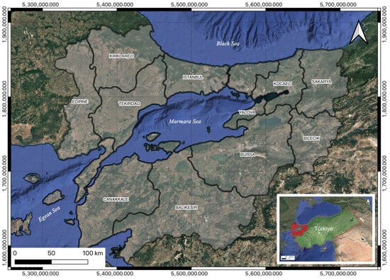
Figure 1. Study area: Marmara Region of Türkiye, highlighted in red at the bottom.

2.2. Flood Risk Analysis with Explainable GeoAI Techniques

When studies on risk analysis are reviewed, it is evident that although different approaches are employed, analyses are generally conducted using fixed data, and risk is modeled based on historical data [14,15,16,17,18,19,20]. Within the scope of this study, a hybrid method was employed, combining the Analytical Hierarchy Process (AHP) with machine learning methods to create the flood risk map. In this context, hazard and vulnerability assessments were carried out to create a flood risk map in the Marmara Region. The raw data used in the production of these maps were collected from both open source platforms and official institutions. Spatial layers of buildings, roads, waterways, and water bodies in the study area were obtained from the OvertureMaps web platform, an open-source spatial data provider. In addition, the administrative boundaries were derived from OpenStreetMap, while land use and land cover (LU/LC) data were sourced from ESRI. Digital Elevation Model (DEM) data with a 30 m resolution were provided by the USGS data portal, and population data were accessed through the TÜİK open data portal. Furthermore, 40-year daily precipitation data were supplied by the General Directorate of Meteorology (MGM), and flood inventory data for the past 50 years were retrieved from the General Directorate of State Hydraulic Works (DSI). Open-source Python software (version 3.14) was used throughout this study for processing, analyzing, and visualizing the data. In this context, the criteria based on the AHP are applied using raster analysis in Python, in line with the specified criteria. In this context, slope, aspect, elevation, flow direction, flow accumulation, waterways proximity, waterbodies proximity, and precipitation analyses were performed using the evaluated criteria. These data were divided into risk classes by processing 30 m resolution raster analyses performed in Python using libraries such as rasterio, GeoPandas, Scipy, Whitebox, PyArrow, matplotlib, pandas, Apache Sedona, and Pyspark.

When generating the AHP-based hazard map, it was assumed that the decision options on the same plane were completely independent of each other [21]. Next, a pairwise comparison matrix was created to calculate the weights of the decision criteria. Using a significance scale that takes values between 1 and n, matrices were created in which the decision options were compared according to the criteria. First, the basic criteria, if any, were considered, followed by the sub-criteria, and finally, all criteria were taken into account. Comparison matrices are square matrices with diagonal elements of 1. The relationship between the pairwise comparison values of two mutual criteria is expressed as $a_{21}$ = ${1/a}_{12}$ (1).

$$A=\left[\begin{array}{ccc}{a}_{11}& \dots & a_{1n}\\ ⋮& \ddots & ⋮\\ a_{n1}& \dots & a_{nn}\end{array}\right]=\left[\begin{array}{ccc}{a}_{11}& \dots & a_{1n}\\ ⋮& \ddots & ⋮\\ {1/a}_{1n}& \dots & a_{nn}\end{array}\right]$$

(1)

First, the cells in each column of the generated comparison matrix are summed, and then each cell in the binary comparison matrix is divided by the initially calculated column sum. With this approach, a normalized matrix is obtained. The normalized matrix is used for calculating the weight vector. The averages in each row of the normalized matrix are calculated, and the weight vector is calculated. In order to determine the priority matrix, the binary comparison matrix and the weight vector must be multiplied (2). Then, the maximum eigenvalue (${\mathsf{\lambda }}_{max}$) is calculated with Formula (3).

$$\left[A{W}_i\right]=\left[A\right]\left[W_i\right]$$

(2)

$${\mathsf{\lambda }}_{max}={\displaystyle \frac{1}{n}}{\sum }_{i=1}^n\left({\displaystyle \frac{{AW}_i}{W_i}}\right)$$

(3)

When these equations are examined, n is the number of criteria, A is the pairwise comparison matrix, and W is the weight vector. The Eigenvector Method (EM) is also known as the method for determining the weight vector of the pairwise comparison matrix [22]. The decision maker may not always be able to make comparisons between consistent pairs, so the Consistency Rate (CR) of the pairwise comparison matrix A is calculated to determine its acceptability [23].

$$CI={\displaystyle \frac{({\mathsf{\lambda }}_{max}-n) }{(n-1)}}$$

(4)

$$CR={\displaystyle \frac{CI}{RI}}$$

(5)

The CI value expressed in the equation is the consistency index. The RI value depends on the number n and represents the random inconsistency index (4). CR is calculated with the CI and RI ratio (5). If the Consistency Ratio (CR) is calculated to be below 10% (0.10), the comparison matrix is considered to have acceptable consistency [24]. The final risk score can be determined (6) according to the weights ($w_i$) and general criteria ($c_i$) obtained from the AHP analysis [25,26]:

$$R={\sum }_{i=1}^n{w}_i\times c_i$$

(6)

While creating the vulnerability map, XGBoost and RF machine learning classification models were used. In this context, before model training, elevation, aspect, plan curvature, profile curvature, drainage density, distance to drainage network, curve number, precipitation, Topographic Wetness Index (TWI), Topographic Rugged Index (TRI), Stream Power Index (SPI), population, and land use classification analyses were performed using open-source Python libraries at a 30 m pixel resolution.

The RF machine learning algorithm is widely used in artificial intelligence studies and is an algorithm that performs supervised classification and regression. RF is a tree-based algorithm that is generally not prone to overfitting and is easy to use [27]. This is because the RF algorithm selects the data in the dataset to form subsets using a random sample selection method. As a result of this selection process, more than one decision tree is created, and thus a forest model consisting of decision trees is formed [27,28]. Training data and a number of feature variables are randomly selected from the training datasets at all decision nodes in each tree in the forest, and after this process, the learning process is carried out for each decision tree. For the results obtained from trees in the forest, if the RF algorithm is used in regression analyses, the average of all predictions is taken; if it is used in classification analyses, the class with the most votes among the predictions is selected, and the classification result is obtained.

Extreme Gradient Boosting (XGBoost), a machine learning algorithm, was developed by Chen and Guestrin [29]. The model is a supervised machine learning method developed based on the fundamental principles of the Gradient Boosting algorithm. The XGBoost algorithm comprises both regression and classification decision trees. It can produce a strong learning algorithm by combining weak learning models. Weak learning models generate regression trees; the success of the algorithm is assessed and used to form the next tree using the residual iteration method. The XGBoost algorithm provides successful results in solving complex problems. The working method of XGBoost and Gradient Boosting algorithms is the same; however, the XGBoost algorithm has features that enable it to work more efficiently and effectively than Gradient Boosting and other estimation algorithms. One of the primary reasons the XGBoost algorithm is a preferred method is that it yields relatively fast results compared to other estimation methods. The memory usage of the XGBoost algorithm is also lower than that of the Gradient Boosting algorithm. It provides fast and successful results by requiring fewer hardware requirements [29].

The performance evaluation of the machine learning models XGBoost and RF enables the assessment of the classification models from various aspects. Each metric measures the model’s tendencies for correct and incorrect classifications, positive and negative predictions, and sensitivity to decision thresholds.

$$Precision={\displaystyle \frac{TP}{TP+FP}}$$

(7)

$$Recall={\displaystyle \frac{TP}{TP+FN}}$$

(8)

$$Accuracy={\displaystyle \frac{TP+TN}{TP+TN+FP+FN}}$$

(9)

$$F_1=2\times {\displaystyle \frac{Precision x Recall}{Precision+Recall}}$$

(10)

SHapley Additive exPlanations (SHAP) analyses are performed using explainable artificial intelligence to compare both models. SHapley values calculate the average contribution of all variables to the result by examining the effects of all possible situations in which they are present or absent from the model [30,31]. In this context, feature-importance bars, dependence plots, force plots, waterfall plots, decision plots, and interaction value parameters were evaluated using SHAP. According to the performance evaluation results, the use of the XGBoost model was deemed appropriate. Using the Ordinary Kriging method with the y_test data from the XGBoost model, a continuous risk surface was created by taking into account the point estimates and spatial relationships within the study area [32]. In this context, a workflow chart containing all stages was created (Figure 2).

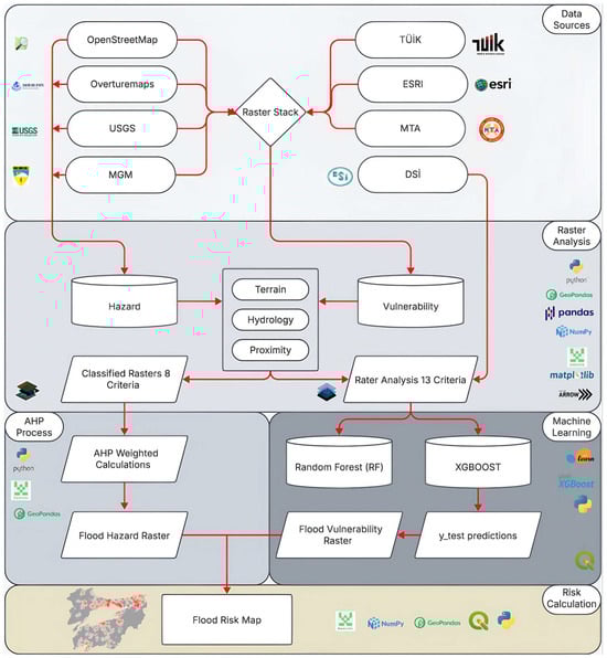
Figure 2. Workflow diagram of the flood risk analysis.

2.3. Flood Hazard Assessment

Determining the criteria affecting the flood risk is one of the first stages of the risk analysis process. Many criteria can be evaluated for flood risk; what is important is how significant the criteria that are determined are in assessing the flood risk. In this context, the criteria affecting risk varied for the hazard and vulnerability maps created to determine the flood risk. The Marmara Region flood risk map incorporates the criteria from both maps. In this context, the factors that can be considered as natural flood hazards were determined (Table 1).

Table 1. Factors affecting flood hazard.

ID	Factor	Data Source	Evaluation
1	Slope	USGS	Hazard
2	Aspect	USGS	Hazard
3	Elevation	USGS	Hazard
4	Flow Direction	USGS	Hazard
5	Flow Accumulation	USGS	Hazard
6	Waterways Proximity	OvertureMaps	Hazard
7	Waterbodies Proximity	OvertureMaps	Hazard
8	Elevation	USGS	Hazard
9	Aspect	USGS	Vulnerability
10	Plan Curvature	USGS	Vulnerability
11	Profile Curvature	USGS	Vulnerability
12	Drainage Density	USGS	Vulnerability
13	Drainage Proximity	USGS	Vulnerability
14	Curve Number	USGS	Vulnerability
15	Precipitation	MGM	Vulnerability
16	Topographic Wetness Index (TWI)	USGS	Vulnerability
17	Topographic Rugged Index (TRI)	USGS	Vulnerability
18	Stream Power Index (SPI)	USGS	Vulnerability
19	Population	TUIK	Vulnerability
20	Land Use	ESRI	Vulnerability
21	Flood Impact	DSİ	Vulnerability

In AHP, decision makers create pairwise comparison matrices by comparing alternatives to each other in the face of complex problems. The weights and rankings of the criteria can be determined by taking the geometric averages of the created matrix [33]. The flood hazard map generation evaluated eight parameters related to natural flood hazards: slope, aspect, elevation, flow direction, flow accumulation, waterways proximity, waterbodies proximity, and precipitation. All criteria and criterion scoring used in the production of the flood hazard map are shown in the figure (Figure 3).

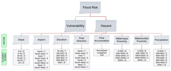
Figure 3. Flood hazard factors (red arrows) and class scores.

The criteria and priorities required for the decision are determined so that the target to be achieved is at the top. The main criteria and sub-criteria are listed under the target to be achieved, while those that can be evaluated as alternatives are placed at the bottom. As the complexity and detail of the problem increase, the number of stages in the hierarchy is also affected. In the created hierarchy, all options are considered independent of each other. When creating a pairwise comparison matrix, matrices suitable for the determined scale are constructed using importance values ranging from 1 to 9. The purpose here is to compare decision options to the criteria and to consider all criteria, taking into account the main criteria and sub-criteria in order [23,34], from equal importance to intermediate values.

The Random Index (RI) value must be known to evaluate consistency. In this context, the RI value is defined as a multidimensional comparison matrix. The RI value was calculated as 1.41 since n = 8 [34]. A scale of importance with values ranging from 1 to 8 was used. A pairwise comparison matrix was created by considering all criteria and comparing decision options according to the criteria: C1: slope, C2: aspect, C3: elevation, C4: flow direction, C5: flow accumulation, C6: waterways proximity, C7: water bodies proximity, and C8: precipitation (Table 2). Comparison matrices are square matrices with diagonal elements of 1. Decision options are compared separately according to each criterion. A pairwise comparison matrix was created by examining the studies in the literature and taking expert opinions. Each criterion was scored according to its importance, and a pairwise comparison matrix was created.

Table 2. Comparison matrix for flood hazard of the region.

Criteria	C1	C2	C3	C4	C5	C6	C7	C8
C1	1	3	1/3	1/5	1/5	1/7	1/7	1/5
C2	1/3	1	1/3	1/7	1/7	1/9	1/9	1/7
C3	3	5	1	1/3	1/3	1/5	1/5	1/3
C4	5	7	3	1	1/3	1/5	1/5	1/3
C5	5	7	3	3	1	1/3	1/3	1/3
C6	7	9	5	5	3	1	1/3	3
C7	7	9	5	5	3	3	1	3
C8	5	7	3	3	3	1/3	1/3	1

When calculating the normalization matrix, a binary matrix is used, which is obtained by dividing each cell value in the matrix by the column total value. In order to calculate the weight vector of each criterion, the average of each row in which the normalized vector is located is calculated (Table 3). In this context, the maximum eigenvalue (λmax) was calculated as 8.8378. RI, CI, and CR values were estimated as 1.41 (for 8 criteria), 0.1197, and 0.0849, respectively. The Consistency Ratio (CR) value was calculated to be 8% in this study. According to research, when the CR value is less than 10%, the comparison matrix is considered to be consistent. As a result, the weights according to AHP were determined as 3% (slope), 2% (aspect), 6% (elevation), 19% (flow direction), 12% (flow accumulation), 23% (waterways proximity), 31% (waterbodies proximity), and 15% (precipitation).

Table 3. Determination of the weight vector from the normalization matrix.

Criteria	C1	C2	C3	C4	C5	C6	C7	C8	Weight (Wi)
C1	0.0303	0.0625	0.0161	0.0113	0.0182	0.0268	0.0400	0.0299	0.0303
C2	0.0101	0.0208	0.0161	0.0081	0.0130	0.0209	0.0120	0.0133	0.0185
C3	0.0909	0.1042	0.0484	0.0189	0.0303	0.0376	0.0400	0.0566	0.0556
C4	0.1515	0.1458	0.1452	0.0566	0.0303	0.0376	0.0400	0.0566	0.0851
C5	0.1515	0.1458	0.1452	0.1697	0.1256	0.0376	0.1200	0.0566	0.1162
C6	0.2121	0.1875	0.2419	0.2829	0.3769	0.1256	0.1200	0.3399	0.2335
C7	0.2121	0.1875	0.2419	0.2829	0.3769	0.3769	0.3600	0.3399	0.3119
C8	0.1515	0.1458	0.1452	0.1697	0.1256	0.0268	0.1200	0.1057	0.1489

Geographical analyses were performed for the criteria determined within the scope of flood hazard. In this context, waterways proximity, aspect, slope, waterbodies proximity, flow direction, precipitation, elevation, and flow accumulation maps were produced (Figure 4).

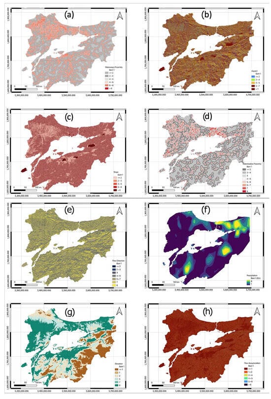
Figure 4. Flood hazard factor maps: (a) waterways proximity, (b) aspect, (c) slope, (d) waterbodies proximity, (e) flow direction, (f) precipitation, (g) elevation, and (h) flow accumulation.

Using all of the hazard criteria, a flood hazard map was produced using the AHP method (Figure 5). In the flood hazard map production process, the “waterways proximity” map was first selected as a reference raster with rasterio.open function of the rasterio library. The reason for this selection was to obtain basic metadata and grid dimensions for the output raster. Then, each criterion raster (waterways proximity, aspect, slope, waterbodies proximity, flow direction, precipitation, elevation, and flow accumulation) was read from the source raster data using rasterio.open. Using the reproject function and the Resampling.nearest function of the rasterio library, the data was resampled in accordance with the transformation and CRS information of the reference raster (EPSG:5637). The weighting (data * weights [key]) process was performed on a numpy array, and the result was collected in a directory. After all criteria were processed, the reference metadata was updated, and the final AHP-weighted flood hazard raster was created in TIFF format using the rasterio.open/dst.write functions.

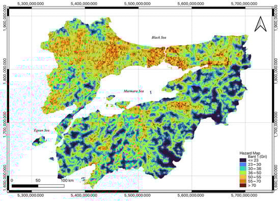
Figure 5. Flood hazard map.

2.4. Flood Vulnerability Assessment

While creating the vulnerability map, XGBoost RF models were preferred. In this context, before model training, elevation, aspect, plan curvature, profile curvature, drainage density, distance to drainage network, curve number, precipitation, Topographic Wetness Index (TWI), Topographic Rugged Index (TRI), Stream Power Index (SPI), population and land use classification analyses were performed using open-source Python libraries at a 30 m pixel resolution (Figure 6). Precipitation data were obtained from MGM on a station basis. In this context, the annual highest daily precipitation value was calculated for each station. Frequency analysis was performed to statistically determine the severity of extreme precipitation events that trigger flood risk and the 100-year recurrence period. In order to model extreme values, the Gumbel distribution was implemented using the gumbel_r function of the Scipy library. A continuous precipitation surface was created by taking into account the point estimates and spatial relationships in the study area with the obtained annual highest precipitation data (mm). Flood inventory data were processed and used with these analyses. Training and test datasets with 13 parameters and a flood inventory spanning the past 50 years were created as raster stacks in the data preprocessing steps.

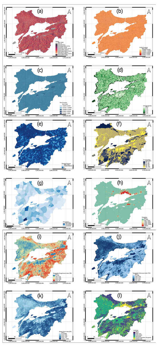
Figure 6. Flood vulnerability factor maps: (a) aspect, (b) profile curvature, (c) plan curvature, (d) drainage density, (e) drainage proximity, (f) curve number, (g) precipitation, (h) population, (i) TRI, (j) TWI, (k) SPI, and (l) land use.

The datasets used in the XGBoost and RF models were evaluated using a 70/30 training and testing ratio. Within the scope of this paper, the flood data obtained from DSI were evaluated as flooded (1) and non-flooded (0) points based on binary classification logic. In order to obtain a realistic distribution, the flooded (1) data were multiplied by 10 times random points at a distance of 200 m from the relevant water source. While producing non-flooded (0) data, a quantity 50 times greater than that of the flooded (1) points was kept in order to obtain a realistic distribution. Machine learning models tend to be biased towards the majority class (non-flooded points (0)). In many classification problems, particularly in environmental or socioeconomic datasets, the distribution of classes is highly imbalanced. This can cause the model to become biased toward the majority class, resulting in poor performance when predicting the minority class. The Random Under-Sampling (RUS) approach is used to prevent this issue. There is no specific rule, as the optimal ratio depends on the degree of class imbalance, dataset size, and model sensitivity. However, several typical strategies and ratio ranges can be applied. In this study, we employed grid search and cross-validation to determine the optimal trade-off between bias reduction and information retention. Increasing the non-flooded points by 50 times initially created an intentional class imbalance. This class imbalance was eliminated using the Random Under-Sampling (RUS) method (at a ratio of 1:50).

Performance evaluations of the generated XGBoost and RF models were performed. Within the scope of performance evaluations, precision, recall, F1 score, area under the ROC curve (AUROC), and binary confusion matrix values were compared. SHapley Additive exPlanations (SHAP) analyses were performed using explainable artificial intelligence to compare both models. SHapley values calculate the average contribution of all variables to the result by examining the effects of all possible situations in which they are present and absent in the model [31]. In this context, feature-importance bars, dependence plots, force plots, waterfall plots, decision plots, and interaction value parameters were evaluated using SHAP. According to the performance evaluation results, the use of the XGBoost model was deemed appropriate. Using the Ordinary Kriging method with the y_test data from the XGBoost model, a continuous risk surface was created, taking into account the point estimates and spatial relationships within the study area [32].

Ordinary Kriging was employed as the spatial interpolation method to estimate the spatial distribution of flood risk indicators across the study area. This method was selected due to its capability to produce unbiased and minimum-variance estimates when the underlying spatial process satisfies the assumptions of second-order stationarity and isotropy. Prior to interpolation, exploratory spatial data analysis was conducted to verify these assumptions. The descriptive statistics and spatial trend analysis indicated that the mean and variance of the flood-related variables (e.g., water depth, inundation frequency, and flood susceptibility index) remained approximately constant across space, confirming the assumption of stationarity. Furthermore, directional semivariograms revealed no pronounced directional dependence, supporting the assumption of isotropy. Given these conditions, Ordinary Kriging was considered appropriate, as the data did not exhibit strong spatial trends that would necessitate Universal Kriging or Regression Kriging approaches. The experimental semivariogram was constructed to capture the spatial autocorrelation structure and subsequently fitted with a theoretical model, ensuring a good representation of the observed spatial dependence in flood risk values.

2.5. Vulnerability Model Performance Evaluation

The generated XGBoost and RF models were evaluated in pairs according to their performance metrics. Within the scope of performance evaluations, precision, recall, F1 score, and AUC values were obtained (Table 4). Although the results are close to each other, the XGBoost model achieved superior performance in terms of accuracy, precision, F1 score, and AUC values.

Table 4. Performance metrics comparison.

ML Model	Accuracy	Precision	Recall	F1 Score	AUC
Random Forest	0.9459	0.9046	0.9930	0.9467	0.9747
XGBoost	0.9493	0.9114	0.9916	0.9498	0.9780

The area under the ROC curve (AUROC) values were compared (Figure 7). The horizontal axis in the graph represents the false positive rate (FPR), the vertical axis represents the true positive rate (TPR). The dashed line represents the random guess line (AUC = 0.5), and the blue curves show the model performance. As the area under the ROC curve increases, the model performance increases. While the RF model had an AUC value of 0.9747, the XGBoost model had an AUC value of 0.9780. In this context, although both models showed good performance, the XGBoost model performed better than the RF model.

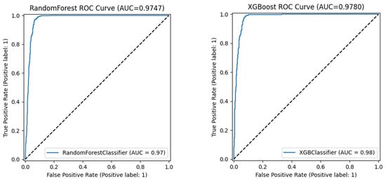
Figure 7. RF and XGBoost ROC curves against random chance level (AUC = 0.5).

Error matrices were obtained for a more comprehensive evaluation of the performance comparisons (Figure 8). Both models can distinguish between the non-flood class (“0”) and the flood class (“1”) with very high accuracy. False negative (FN) values were recorded as 5 for RF and 6 for XGBoost. False positive (FP) values were 75 for RF and 69 for XGBoost, meaning that the XGBoost model has a lower false prediction rate. When all these results are evaluated, the XGBoost model stands out in the comparison of the two models used.

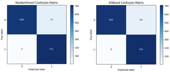
Figure 8. RF and XGBoost confusion matrix. The top-left box displays the number of true positives (TPs), and the box beneath it displays the number of false positives (FPs). The top-right box displays the number of false negatives (FNs), and the bottom-right box displays the number of true negatives (TNs). The color bar represents the number of test data.

According to the performance evaluation results, the use of the XGBoost model was deemed appropriate. The obtained y_test point data were processed using the Ordinary Kriging method in QGIS, an open-source GIS software (version 3.38), due to the large study area and the limited hardware resources available. With this method, a continuous risk surface and flood vulnerability map were created at a 30 m resolution, taking into account the point estimates and spatial relationships within the study area (Figure 9).

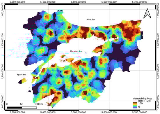
Figure 9. Flood vulnerability map.

To explain the feature importance and the decision mechanisms within the model, SHapley Additive exPlanations (SHAP) analyses were performed using explainable artificial intelligence. SHapley values assess the impact of all possible situations in which all variables are either present or absent from the model, quantifying their average contribution to the result. When the SHAP values belonging to the XGBoost model are evaluated and the produced feature importance and global summary graphs are examined, it is found that drainage proximity has the highest effect on the model. Elevation, land use, and precipitation parameters also showed superior effects in the model compared to other parameters. In order to explain the feature importance and decision mechanisms within the model, the TreeExplainer function of the SHAP library was used for each model and for 100 randomly selected samples. Feature importance and global summary graphs produced within the scope of SHAP values belonging to the XGBoost model were created (Figure 10).

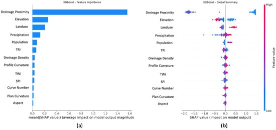
Figure 10. XGBoost SHAP values: (a) feature importance and (b) global summary.

3. Results and Discussion

GeoAI-based risk mapping in the Marmara Region provides analysis advantages over traditional methods, particularly in multiple datasets and large-scale regions. The hybrid use of AHP and XGBoost in the Marmara Region scale combines expert knowledge and data-driven learning at the same point, increasing both the interpretability and estimation accuracy of the risk map. While the criterion weights determined by experts in AHP provide the model with a guiding role, XGBoost fine-tunes these weights with non-linear relationships and local differences in the data. Thus, the fixed, rule-based decision boundaries of AHP alone are exceeded, and data-based patterns are learned, while the risk of overfitting in XGBoost alone is balanced with the predefined weights of AHP.

When assessing risk, hazard, and vulnerability, the criteria should be evaluated together. This approach, which is frequently used in risk assessment, has been expressed by many researchers as “Risk = Hazard × Vulnerability” [35,36,37,38]. In this context, the hazard and vulnerability maps are produced by using the rasterio library at the same pixel resolution and multiplying both raster data to obtain the Marmara Region flood risk map. In this process, first, an environment is prepared for reading and writing raster data with the osgeo.gdal library and osgeo.osr function, which is the Python binding of GDAL. The pixel values of the generated raster data (flood hazard map and flood vulnerability map) are accessed with the “osgeo.gdal” and “numpy” libraries. Afterwards, risk scores are generated by multiplying each pixel by each other (preserving no-data values) using the numpy library. The final risk map created using the “osgeo.gdal” library is saved as a raster (Figure 11).

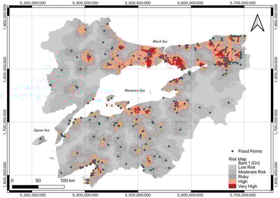
Figure 11. Flood risk map.

As a result, considering the variable topography, hydrography, and settlement model of the Marmara Region, the hybrid approach provides both high AUC/F₁ scores and prepares a transparent, criterion-based explanation for decision makers. Thus, both reliable and traceable flood risk maps are obtained in a wide area.

Predetermining expert-based criteria weights using AHP and integrating XGBoost’s data-driven, non-linear learning power provides approximately a 5% increase in AUC, approximately a 4% increase in accuracy, and more accurate predictions in high uncertainty regions compared to rule-based AHP alone. It is demonstrated that the hybrid approach, which combines both domain knowledge and data-driven pattern recognition, provides significant superiority in both explainability and generalization ability compared to the methods used alone.

Among the geographical criteria weighted using the AHP method, proximity to waterbodies accounted for 31%, proximity to waterways for 23%, flow direction for 19%, and precipitation for 15%. This distribution revealed that hydraulic processes are the primary factors contributing to flood hazard in the region. In this context, the maximum eigenvalue (λmax) is calculated as 8.8378. The RI value is calculated as 1.41, the CI value as 0.1197, and the CR value as 0.0849. In this study, the Consistency Rate (CR) value is calculated to be 8%, and according to research, when the CR value is less than 10%, the comparison matrix is considered to be consistent. In this case, a consistent comparison matrix is obtained. According to AHP, the weights are determined as 3% (slope), 2% (aspect), 6% (elevation), 19% (flow direction), 12% (flow accumulation), 23% (waterways proximity), 31% (waterbodies proximity), and 15% (precipitation).

In the machine learning algorithms used within the scope of flood vulnerability, RF is relatively resistant to overfitting while making decisions with the majority vote of many trees, while XGBoost learns complex patterns with fine-tuning since it corrects the error residuals each time with Gradient Boosting. In this study, both models yielded an AUC above 98% and an F1 score of nearly 95%. However, XGBoost demonstrated superior generalization ability, achieving an AUC of approximately 0.003, an F1 score of approximately 0.002, and a better false positive/negative balance compared to the RF model in the test set.

The XGBoost model showed superior performance compared to the RF model, achieving an accuracy of 0.9493, a precision of 0.9114, an F1 score of 0.9498, and an AUC value of 0.9780. When the area under the ROC curve (AUROC) values were compared, the RF model had a value of 0.9747, whereas the XGBoost model calculated a higher area with a value of 0.9780, indicating better performance. While the high scores in the training set (AUC > 0.99, F1 > 0.97) carried the risk of overfitting, the approximately equivalent performance in the test set (an AUC of approximately 0.97–0.98 and an F1 score of approximately 0.95) confirmed the generalization ability of the models. When both models are evaluated for both the non-flooding “0” and flooding “1” classes, the false negative (FN) values obtained are 5 for RF and 6 for XGBoost. The false positive (FP) values are 75 for RF and 69 for XGBoost; in other words, the false prediction rate of the XGBoost model is lower. When all these results are evaluated and the two models are compared, XGBoost stands out.

As a result of SHapley Additive exPlanations (SHAP) analyses using explainable artificial intelligence, the effects of all possible situations where all variables are present or absent in the model are examined by the SHAP values of the XGBoost model. The evaluation of SHAP values from the XGBoost model, as depicted in the decision plot, indicates that drainage proximity exerted the most significant influence on the model (Figure 12). Elevation, land use, and precipitation parameters also played a significant role in determining flood vulnerability in the model, compared to other parameters. Topographic factors determined the direction and speed of water flow and increased flood vulnerability in high-slope valleys. Socioeconomic variables (population density and land use classes) increased flood vulnerability in densely populated areas by affecting the infrastructure status. The combined effects of nature and human settlement are evident in the model.

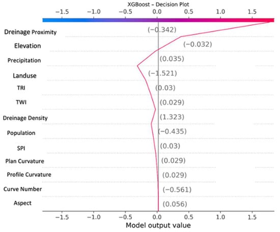
Figure 12. SHAP decision plot; pink line indicates SHAP value.

Lacking drainage infrastructure in the region may increase vulnerability to flooding. The SHAP decision plot also validates that drainage proximity highly contributes to the flood risk model. Floods are frequently encountered in the district centers of the European and Anatolian sides of Istanbul, the strait/coastal line of Çanakkale, the coastal areas of the Aegean Sea and the coastal areas of the Marmara Sea of Balıkesir province, the south of the Kırklareli province, the Uludağ region of Bursa province, the city center and coastal areas of the Yalova province, the central districts and the Black Sea coastal areas of the Sakarya province, and the city center and the Marmara Sea coasts of the center of the Kocaeli province. There are high- and very high-risk clusters on the flood risk map for this specified region. Flood occurrences within the Bilecik and Eskişehir surroundings have exhibited a limited distribution, and flood events have been rare in the past. These areas are also included in the low and medium-risk groups on the flood risk map. Flood disasters have historically occurred in the western parts of Edirne Province and Tekirdağ Province, and these areas are identified as high-risk and risky on the flood risk map. Bursa province, the Bilecik border regions, the inner parts of Çanakkale province, and Çanakkale’s European side are designated as low- and medium-risk regions on the map. The risk map exhibits a strong correlation with past flood events. The model effectively captures past flood data and yields accurate high-risk predictions. The low number of missed flood disasters yielded a high recall (0.9916).

Multi-Criteria Decision Making (MCDM) methods are frequently utilized in risk analysis because they offer advantages such as consistency in judgment [39], systematization of criteria [40], and convenience for integration in GIS [41]. Flood risk assessment typically involves considering both the susceptibility to flooding and the consequences of flooding [42]. This is often achieved by integrating the fundamental components of flood risk, including flood hazard, exposure, and vulnerability [43]. A popular MCDM technique, AHP, can be utilized in the GIS setting to integrate these components. The comprehensiveness of the analysis is enhanced by incorporating machine learning and MCDM, as this combined approach has been shown to provide useful results. Machine learning techniques are applied to generate the hazard map, which is proposed as a potential option for constructing the flood vulnerability map [44]. Additionally, the evaluation is further enhanced by utilizing SHAP, an explainable AI method, to develop a highly accurate flood risk analysis approach. Machine learning tools and traditional methods are not competitive replacements but rather highly complementary when integrated with AI and MCDM for flood risk analysis.

Machine learning techniques, particularly XGBoost, are applied to build risk components, such as hazard and vulnerability maps, delivering superior predictive performance. For instance, this approach provides approximately a 5% increase in AUC and improved accuracy compared to rule-based AHP alone. Furthermore, XAI is used to ensure transparent, criterion-based explanations. Despite these strengths, these specialized models face critical limitations regarding their application beyond the training context. Transferability is restricted by data distribution shift and context-dependent relationships specific to the study area. Generalization to future scenarios is challenging due to temporal non-stationarity, as models trained on past flood events often fail to account for the evolving impacts of global issues, like climate change. The developed risk analysis model is scalable to broader geographical extents, as this study covers a large area, including 11 cities of the Marmara Region.

4. Conclusions

Several parameters have been examined in conjunction with the research conducted to create a flood risk map in the Marmara Region. When the research conducted in the study area and the information obtained from official institutions are examined, it is observed that 570 flood disasters occurred in the Marmara Region between 1975 and 2025. Additionally, it has been observed that flood disasters have occurred near regions where reclamation work has been carried out in recent floods. A hybrid model has been created by examining the flood risk, flood hazard, and flood vulnerability. This study was carried out in the open source software Python, and the GeoAI approach was adopted by using the RF and Extreme Gradient Boosting (XGBoost) models from machine learning methods. According to the performance evaluation results, the use of the XGBoost model was deemed appropriate. When the Marmara Region flood risk map is examined, it is evident that the areas of very high and high risk overlap with the locations where floods actually occur, confirming the accuracy of the flood risk map produced. It also demonstrates that the model accurately captures past flood data and that high-risk predictions are reliable. The low number of missed flood disasters yielded results consistent with high recall. The proposed methodology can be enhanced by incorporating catchment areas for the water resources and by augmenting the training data for the model. However, the inventory data acquired from the public authorities is stored as point vector data. Data quality issues can be named as a limitation of this study.

In the context of disaster preparedness, automatic water level meters and SMS/application-based alarm systems can be installed in regions with very high and high risk. Drainage investments, such as rainwater lines, rain gardens, and infiltration pits, should be prioritized in high-risk urban areas. Areas that the model identifies as medium risk but contain past flood points (false negatives, FN) can be verified through field inspections. New parameters can be added to the model, and the number of criteria used in the model can be increased. Zoning plans and emergency response plans should be updated in accordance with this map layer; construction restrictions may be considered, especially in “very high” zones. In this study, various machine learning algorithms were employed to assess flood risk in the Marmara Region, and their accuracies were compared. Hazard was weighted with the AHP, an MCDM method, and a hybrid approach was adopted. The accuracy of the developed model is significantly increased when applying different methods and the proposed hybrid approach.

References

- FEMA Federal Emergency Management Agency (FEMA). Guide for All-Hazard Emergency Operations Planning. State and Local Guide (SLG) 101. Available online: https://www.fema.gov/pdf/plan/glo.pdf (accessed on 27 October 2025).
- UNDRR United Nations Office for Disaster Risk Reduction (UNDRR). The Sendai Framework Terminology on Disaster Risk Reduction. “Disaster”. Available online: https://www.undrr.org/terminology/disaster (accessed on 27 October 2025).
- Khantong, S.; Sharif, M.N.A.; Mahmood, A.K. An Ontology for Sharing and Managing Information in Disaster Response: An Illustrative Case Study of Flood Evacuation. Int. Rev. Appl. Sci. Eng. 2020, 11, 22–33. [Google Scholar] [CrossRef][Green Version]
- Samela, C.; Manfreda, S.; Paola, F.D.; Giugni, M.; Sole, A.; Fiorentino, M. DEM-Based Approaches for the Delineation of Flood-Prone Areas in an Ungauged Basin in Africa. J. Hydrol. Eng. 2016, 21, 06015010. [Google Scholar] [CrossRef]
- Akyel, R. Disaster Management in Turkish Public Administration. Çukurova Üniversitesi Sos. Bilim. Enstitüsü Derg. 2005, 14, 15–29. [Google Scholar]
- Erkal, T.; Değerliyurt, M. Disaster Management in Turkey. East. Geogr. Rev. 2009, 14, 147–164. [Google Scholar]
- Dölek, İ. Identification of the Areas Susceptible to Flooding and Overflows in Sungu and its Surrounding (Muş). Marmara Coğrafya Derg. 2015, 31, 258–280. [Google Scholar] [CrossRef]
- Adnan, M.S.G.; Abdullah, A.Y.M.; Dewan, A.; Hall, J.W. The Effects of Changing Land Use and Flood Hazard on Poverty in Coastal Bangladesh. Land Use Policy 2020, 99, 104868. [Google Scholar] [CrossRef]
- Batur, E.; Maktav, D. Floodplain Assessment with the Integration of Remote Sensing and GIS: Meric River Case Study. Havacılık Ve Uzay Teknol. Derg. 2012, 5, 47–54. [Google Scholar]
- Utlu, M. Flood Hazard Analysis Based on Different Resolution Data Resources: A Case of Biga River Basin. Ph.D. Thesis, İstanbul University, İstanbul, Türkiye, 2019. [Google Scholar]
- El Bilali, A.; Taleb, A.; Boutahri, I. Application of HEC-RAS and HEC-LifeSim Models for Flood Risk Assessment. J. Appl. Water Eng. Res. 2021, 9, 336–351. [Google Scholar] [CrossRef]
- TURKSTAT. Population Projections, 2023–2100. Available online: https://data.tuik.gov.tr/Bulten/Index?p=Nufus-Projeksiyonlari-2023-2100-53699 (accessed on 29 October 2025).
- Kömüşçü, Ü.A.; Çelik, S.; Ceylan, A. Rainfall analysis of the flood event that occurred in Marmara Region on 8–12 September 2009. CBD 2011, 9, 209–220. [Google Scholar] [CrossRef]
- Bandrova, T.; Zlatanova, S.; Konecny, M. Three-Dimensional Maps for Disaster Management. ISPRS Ann. Photogramm. Remote Sens. Spat. Inf. Sci. 2012, I-4, 245–250. [Google Scholar] [CrossRef]
- Bozkurt, Ö.; Çiçekdağı, H.İ. Criteria Prioritization with the Best-Worst Method (BWM) in Risk Reduction Investments after the Provincial Disaster Risk Reduction Plans (IRAP). Afet Ve Risk Derg. 2022, 5, 109–121. [Google Scholar] [CrossRef]
- Dayanır, H.; Çınar, A.K.; Akgün, Y.; Çorumluoğlu, Ö. Post-Disaster Temporary Shelter Area Selection and Planning by Using Delphi Method: Izmir/Seferihisar Case. Doğ Afet Çev Derg 2022, 8, 87–102. [Google Scholar] [CrossRef]
- Ergünay, O. Natural Disasters and Sustainable Development; Abant İzzet Baysal Üniversitesi: Bolu, Türkiye, 2009. [Google Scholar]
- Fan, Y.; Wen, Q.; Wang, W.; Wang, P.; Li, L.; Zhang, P. Quantifying Disaster Physical Damage Using Remote Sensing Data—A Technical Work Flow and Case Study of the 2014 Ludian Earthquake in China. Int. J. Disaster Risk Sci. 2017, 8, 471–488. [Google Scholar] [CrossRef]
- Koçkan, Ç. Natural Disaster Risk Management; Dokuz Eylül Üniversitesi: İzmir, Türkiye, 2015. [Google Scholar]
- Ocak, F.; Bahadir, M. Creating the Sample Flood Risk Model and Flood Risk Analysis of Rivers in Unye. J. Acad. Soc. Sci. Stud. 2020, 13, 499–524. [Google Scholar] [CrossRef]
- Yildirim, R.E. Development of a semi-dynamic flood prediction model based on geographic information systems. Ph.D. Thesis, Ondokuz Mayıs University, Samsun, Türkiye, 2023. [Google Scholar]
- Saaty, T.L. The Analytic Hierarchy Process; McGraw-Hill: Columbus, OH, USA, 1980. [Google Scholar]
- Wang, Y.-M.; Liu, J.; Elhag, T.M.S. An Integrated AHP–DEA Methodology for Bridge Risk Assessment. Comput. Ind. Eng. 2008, 54, 513–525. [Google Scholar] [CrossRef]
- Saaty, T.L. Decision Making—The Analytic Hierarchy and Network Processes (AHP/ANP). J. Syst. Sci. Syst. Eng. 2004, 13, 1–35. [Google Scholar] [CrossRef]
- Hajkowicz, S.; Collins, K. A Review of Multiple Criteria Analysis for Water Resource Planning and Management. Water Resour. Manag. 2007, 21, 1553–1566. [Google Scholar] [CrossRef]
- Ekmekcioğlu, Ö.; Koc, K.; Özger, M. District Based Flood Risk Assessment in Istanbul Using Fuzzy Analytical Hierarchy Process. Stoch. Environ. Res. Risk Assess. 2021, 35, 617–637. [Google Scholar] [CrossRef]
- Breiman, L. Random Forests. Mach. Learn. 2001, 45, 5–32. [Google Scholar] [CrossRef]
- Liaw, A.; Wiener, M. Classification and Regression by randomForest. R News 2002, 2/3, 18–22. [Google Scholar]
- Chen, T.; Guestrin, C. XGBoost: A Scalable Tree Boosting System. In Proceedings of the 22nd ACM SIGKDD International Conference on Knowledge Discovery and Data Mining, San Francisco, CA, USA, 13–17 August 2016; Association for Computing Machinery: New York, NY, USA, 2016; pp. 785–794. [Google Scholar]
- Lundberg, S.M.; Lee, S.-I. A Unified Approach to Interpreting Model Predictions. In Proceedings of the 31st International Conference on Neural Information Processing Systems, Long Beach, CA, USA, 4–9 December 2017; Curran Associates Inc.: Red Hook, NY, USA, 2017; pp. 4768–4777. [Google Scholar]
- Mete, M.O.; Yomralioglu, T. A Hybrid Approach for Mass Valuation of Residential Properties Through Geographic Information Systems and Machine Learning Integration. Geogr. Anal. 2023, 55, 535–559. [Google Scholar] [CrossRef]
- Koyuncu, Z.; Ekmekcioğlu, Ö. Generating the Flood Susceptibility Map for Istanbul with GIS-Based Machine Learning Algorithms. Doğ Afet Çev Derg 2024, 10, 1–15. [Google Scholar] [CrossRef]
- Hammami, S.; Zouhri, L.; Souissi, D.; Souei, A.; Zghibi, A.; Marzougui, A.; Dlala, M. Application of the GIS Based Multi-Criteria Decision Analysis and Analytical Hierarchy Process (AHP) in the Flood Susceptibility Mapping (Tunisia). Arab. J. Geosci. 2019, 12, 653. [Google Scholar] [CrossRef]
- Saaty, T.L. How to Make a Decision: The Analytic Hierarchy Process. Eur. J. Oper. Res. 1990, 48, 9–26. [Google Scholar] [CrossRef]
- Wisner, B.; Blaikie, P.; Cannon, T.; Davis, I. At Risk: Natural Hazards, People’s Vulnerability and Disasters, 2nd ed.; Routledge: London, UK, 2003; ISBN 978-0-203-71477-5. [Google Scholar]
- Masood, M.; Takeuchi, K. Assessment of Flood Hazard, Vulnerability and Risk of Mid-Eastern Dhaka Using DEM and 1D Hydrodynamic Model. Nat. Hazards 2012, 61, 757–770. [Google Scholar] [CrossRef]
- Dandapat, K.; Panda, G.K. Flood Vulnerability Analysis and Risk Assessment Using Analytical Hierarchy Process. Model. Earth Syst. Environ. 2017, 3, 1627–1646. [Google Scholar] [CrossRef]
- Chakraborty, S.; Mukhopadhyay, S. Assessing Flood Risk Using Analytical Hierarchy Process (AHP) and Geographical Information System (GIS): Application in Coochbehar District of West Bengal, India. Nat. Hazards 2019, 99, 247–274. [Google Scholar] [CrossRef]
- Koczkodaj, W.W.; Magnot, J.-P.; Mazurek, J.; Peters, J.F.; Rakhshani, H.; Soltys, M.; Strzałka, D.; Szybowski, J.; Tozzi, A. On Normalization of Inconsistency Indicators in Pairwise Comparisons. Int. J. Approx. Reason. 2017, 86, 73–79. [Google Scholar] [CrossRef]
- Ishizaka, A.; Labib, A. Analytic Hierarchy Process and Expert Choice: Benefits and Limitations. OR Insight 2009, 22, 201–220. [Google Scholar] [CrossRef]
- Malczewski, J.; Rinner, C. Multicriteria Decision Analysis in Geographic Information Science. In Advances in Geographic Information Science; Springer: Berlin/Heidelberg, Germany, 2015; ISBN 978-3-540-74756-7. [Google Scholar]
- Abedi, R.; Costache, R.; Shafizadeh-Moghadam, H.; Pham, Q.B. Flash-Flood Susceptibility Mapping Based on XGBoost, Random Forest and Boosted Regression Trees. Geocarto. Int. 2022, 37, 5479–5496. [Google Scholar] [CrossRef]
- Luu, C.; Tran, H.X.; Pham, B.T.; Al-Ansari, N.; Tran, T.Q.; Duong, N.Q.; Dao, N.H.; Nguyen, L.P.; Nguyen, H.D.; Thu Ta, H.; et al. Framework of Spatial Flood Risk Assessment for a Case Study in Quang Binh Province, Vietnam. Sustainability 2020, 12, 3058. [Google Scholar] [CrossRef]
- Bui, Q.D.; Luu, C.; Mai, S.H.; Ha, H.T.; Ta, H.T.; Pham, B.T. Flood Risk Mapping and Analysis Using an Integrated Framework of Machine Learning Models and Analytic Hierarchy Process. Risk Anal. 2023, 43, 1478–1495. [Google Scholar] [CrossRef]
Disclaimer/Publisher’s Note: The statements, opinions and data contained in all publications are solely those of the individual author(s) and contributor(s) and not of MDPI and/or the editor(s). MDPI and/or the editor(s) disclaim responsibility for any injury to people or property resulting from any ideas, methods, instructions or products referred to in the content. |
© 2025 by the authors. Licensee MDPI, Basel, Switzerland. This article is an open access article distributed under the terms and conditions of the Creative Commons Attribution (CC BY) license (https://creativecommons.org/licenses/by/4.0/).