Abstract
This study investigates the integration of non-economic policies into the framework for assessing macroeconomic coherence as applied by the Chinese government, with a particular focus on green policies. We examine the impact of non-economic factors on social disagreement and investor disagreement (expectations), and how these influences interact with macroeconomic regulation, employing both empirical evidence and dynamic stochastic general equilibrium (DSGE) theoretical models. In the basic analysis section, we merge statistical data on social divergence with policy implementation, utilizing multiple regression and deep neural network models. Our findings provide direct evidence that non-economic policies significantly regulate social sentiment. Additionally, theoretical analyses using contagion models, grounded in real textual data on social and investor divergence, demonstrate that expectations of social sentiment can ultimately affect economic variables. In the extended analysis, we enhance the classic DSGE model to delineate the pathways through which non-economic policies impact the macroeconomy. Drawing from our analyses, we propose specific optimization measures for non-economic policies. The results indicate that targeted policy optimization can effectively manage social disagreement, thereby shaping expectations and harmonizing non-economic with economic policy initiatives. This alignment enhances the coherence of macroeconomic policy interventions. The innovative contribution of this study lies in its provision of both theoretical and empirical evidence supporting the formulation of non-economic policies for the first time, alongside specific recommendations for improving the consistency of macroeconomic policies.
1. Introduction
During the 2023 Central Economic Work Conference, the Chinese government underscored the importance of maintaining consistent macroeconomic policies and, for the first time, introduced a strategy to incorporate non-economic policies into the evaluation framework for macroeconomic policy alignment. The subsequent “Opinions of the State Council on Strengthening Supervision, Preventing Risks, and Promoting the High-Quality Development of the Capital Market” in 2024 reiterated the necessity of assessing the impacts of both major economic and non-economic policies on capital markets as part of the macroeconomic policy orientation evaluation. This initiative aims to elevate the quality of economic growth through enhanced expectation management, improved economic communication, and effective guidance of public sentiment. Although non-economic policies do not directly control economic activities, they significantly shape positive market expectations, thereby synergizing with macroeconomic policies to foster economic recovery and growth.
As articulated in various governmental documents from China, non-economic policies are distinguished by their independence from fiscal controls as the primary mechanism; nonetheless, they effectively bolster market confidence and enhance the efficacy of economic policy implementation. Despite the increasing focus on non-economic policies, the mechanisms through which they influence economic performance remain inadequately understood. To date, there have been no comprehensive studies elucidating the effects of non-economic policies on economic dynamics. Furthermore, the optimization of the formulation and allocation of such policies remains a pressing challenge.
This study focuses on the theme of “green environmental protection” and explores how non-economic policies influence real-world social disagreements. Utilizing advanced big data techniques, this research aggregates millions of posts and comments related to environmental issues from Sina Weibo, providing valuable insights into the mechanisms through which these policies exert their effects.
In the foundational phase of this study, we propose an evidence-based transmission mechanism linking social disagreements, investor disagreements, and announcements of non-economic policies. Specifically, an increase in the number of central government regulations, departmental normative documents, industry regulations, and administrative approval decisions over the past five days is found to significantly reduce social disagreements. While the coefficients for the number of departmental work documents, joint agency documents, State Council normative documents, and judicial interpretations are positive, the interactions among these factors—such as between the number of publications and departmental work documents, departmental regulations, and joint agency documents—can be further optimized. These interactions present a more effective strategy for managing social disagreements. Additionally, social disagreements and investor disagreements exhibit relative independence; although there is no immediate correlation between the two, social disagreements do influence investor behavior over the long term. In summary, the transmission of social disagreements demonstrates that non-economic policies, while not directly linked to economic variables, can significantly impact economic outcomes.
In the subsequent phase of this research, we integrate these empirical findings into a Dynamic Stochastic General Equilibrium (DSGE) model. Building upon the classic DSGE framework, we incorporate non-economic policies and social disagreements into the behavioral mechanisms. Within this framework, non-economic policies respond to economic policies and past anomalies in social disagreements, while social disagreements are shaped by both non-economic policies and their own lagged values. Moreover, investor expectations and stock price forecasts are influenced to some degree by social disagreements. Simulations and impulse response analyses indicate that incorporating social disagreements and non-economic policies into the DSGE model enhances its capacity to capture actual stock price fluctuations, while interventions via non-economic policies can prolong the effectiveness of positive economic policies.
This study contributes to the literature in three significant ways. First, it establishes a novel sentiment-based framework that integrates regulatory policies, social disagreements, and investor behavior, providing empirical evidence of the impact of non-economic policies on economic factors. Second, by embedding this framework within the DSGE model, the study offers a theoretical foundation for government policy formulation. Finally, by exploring the complex relationship between non-economic policies and social disagreements, it provides actionable recommendations for enhancing policy coherence and optimizing decision-making processes.
This paper is structured as follows: Section 2 reviews pertinent studies to provide theoretical support for the model; Section 3 outlines the research design, including data sources, variable indicators, and calculation methods; Section 4 presents empirical evidence demonstrating how non-economic policies can guide economic factors; Section 5 integrates these findings into the DSGE model for comprehensive analysis; Section 6 offers policy recommendations; and the concluding section summarizes this study’s key findings and suggests directions for future research.
2. Literature Review
The literature relevant to this study primarily encompasses two domains: research on investor disagreement and investigations related to macroeconomic policy interventions.
2.1. Investor Disagreement
Investor sentiment and the divergence of opinions significantly influence economic dynamics. The aspect most pertinent to this research is the emergence of investor disagreement. According to the classical economic assumption of homogeneous expectations, the presence of opinion divergence indicates a deviation from the anticipated return and risk variance of a particular asset over a defined holding period, as articulated by Sharpe (1964) []. Mechanistically, factors such as the gradual dissemination of information, limited attentional capacities, and varying risk preferences elucidate the origins of investor disagreement (Hong & Stein, 2007; Zhang, 2002) [,]. More broadly, the heterogeneous interpretations of information play a crucial role in driving sentiment divergence (Wu, 2022) [], a perspective supported by empirical findings from Giacomini et al. (2020) []. Consequently, the precision of measuring sentiment disagreement is intricately linked to the interpretation of informational heterogeneity.
The measurement of investor disagreement has been a central focus of academic inquiry. Mainstream methodologies encompass analysis of disagreement in analyst forecasts (Kim et al., 2014) [], trading volume-based disagreement indicators (Shi & Li, 2012; Liu & Zhu, 2018) [,], and the divergence among mutual funds (Jiang & Sun, 2014) []. However, advancements in computational technologies and the advent of big data now permit the assessment of sentiment among a large number of individual investors, thereby allowing for a more nuanced calculation of disagreement that accurately reflects heterogeneous interpretations of information. A notable illustration of this trend is Cookson & Niessner’s (2020) [] study, which utilized social media data to analyze individual investor sentiment by constructing sentiment and disagreement indicators from StockTwits, marking a pivotal shift in sentiment research towards the utilization of personal investor data. Similar methodologies have been adopted by Wang et al. (2022) [] and Anthony et al. (2022) [].
Liu et al. (2023) [] introduced social disagreement and non-investor disagreement, showing that social disagreement influences investor disagreement by facilitating information and emotional transmission, thus affecting asset pricing through various channels.
2.2. Macroeconomic Policy and Economic Regulation
Economic policy, often described as the “visible hand”, plays a pivotal role in regulating economic activities. Since the emergence of Keynesian economics, government intervention has become a foundational principle of macroeconomic theory. For instance, Friedman (1968) [] emphasized the necessity of stable monetary growth for achieving long-term economic stability and mitigating cyclical fluctuations. Mankiw et al. (1992) [] demonstrated that government policies that foster education and technological innovation directly enhance human capital and technological capacity, thereby promoting economic growth. Additionally, Kydland and Prescott (1977) [] underscored the significance of policy time consistency for its effectiveness.
Addressing economic policy uncertainty, Liu et al. (2023) [] examined its impact on financing efficiency. Chen (2021) [] highlighted the necessity of aligning demand-side management with aggregate demand for effective macroeconomic regulation. Zhang (2023) [] argued that traditional macroeconomic policies in China are losing efficacy due to behavioral changes among economic agents, necessitating a long-term analysis of specific policy implementation strategies.
2.3. The Interplay Between DSGE and Behavioral Economics
Keynesian “animal spirits” provide a framework for understanding the influence of non-rational factors on market decision-making. Azariadis (1981) [] was among the first to incorporate “animal spirits” into the Dynamic Stochastic General Equilibrium (DSGE) model, with subsequent enhancements by Farmer & Guo (1994) [] and Benhabib & Farmer (1994) []. Nevertheless, these studies continued to operate within the confines of rational expectations. Sargent (1993) [] was the first to introduce bounded rationality into macroeconomic models. De Grauwe (2011) [] proposed that economic agents alternate between optimistic and pessimistic forecasting rules and adjust these based on actual outcomes, thereby providing a mechanism to capture “animal spirits”. Wen (2017) [] integrated these characteristics into the DSGE model, enabling the endogenous modeling of boom-and-bust cycles in stock markets, wherein changes in economic policy significantly influence investor sentiment, ultimately affecting stock prices and the broader economy. Liu et al. (2023) [] incorporated investor and entrepreneur confidence into the DSGE framework, demonstrating that government economic policies must consider confidence factors to enhance their efficacy.
2.4. Review of the Literature
A synthesis of the literature on investor disagreement, social disagreement, and macroeconomic policy regulation yields several key insights: (1) Employing big data to analyze sentiment disagreement is vital for enhancing the credibility of research findings. (2) Social disagreement, as an expanded form of investor disagreement, is more intricately linked to non-economic policies, effectively addressing the waning efficacy of traditional macroeconomic regulation. (3) The structured role of non-economic policies remains largely unexamined, highlighting a significant gap in the current research landscape. (4) Within the context of DSGE models, the integration of social sentiment factors and non-economic policies is unprecedented.
Consequently, it is both necessary and urgent to investigate how “non-economic policies can influence economic operations by guiding social sentiment and alleviating Investor Disagreement, thus achieving synchronization with macroeconomic objectives”.
3. Research Design
3.1. Research Framework
The research framework illustrated in Figure 1 seeks to investigate the ways in which the Chinese government employs non-economic policies to shape public expectations and emotions, ultimately aiming to regulate the economy. However, there remains a significant gap in both theoretical and empirical studies that substantiate this framework. To address this deficiency, we aim to provide evidence for the efficacy of these policies through a dual approach involving empirical data and theoretical modeling.
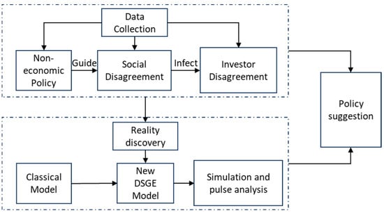
Figure 1.
Research framework.
Firstly, from an empirical standpoint, we assembled a comprehensive and stratified dataset to analyze the interplay between social disagreement and investor disagreement. By applying a series of analytical models, we explored the extent to which non-economic policies influence social disagreement. Furthermore, we examined the prerequisites and contagion relationship of social disagreement on investor disagreement, thereby elucidating the regulatory effect of non-economic policies on the economy. This investigation not only verifies the practical impacts of the policies but also lays an empirical foundation for our theoretical framework.
Secondly, leveraging the empirical findings, we adapted the traditional Dynamic Stochastic General Equilibrium (DSGE) model to integrate non-economic policies and social disagreement as critical non-economic factors. Through simulation and modeling, we assess the potential regulatory effects of non-economic policies on economic dynamics, thereby providing theoretical validation for the construction of our research framework.
Finally, based on specific empirical results and the support of our theoretical model, we propose a series of policy recommendations designed to inform actual policy formulation.
3.2. Data Sources
The data utilized in this study originate from four principal sources: public market data, web-scraped data, the CNRDS database, and the PKULaw database. Public market data were primarily sourced from the Tonghuashun stock trading software, specifically targeting stocks within the environmental protection sector. The web-scraped data were obtained from the Sina Weibo platform using Python-based scraping scripts, capturing posts and comments related to themes such as “green”, “environmental protection”, “low carbon”, and “new energy”. The CNRDS database provides insights into interactions between companies in the environmental protection sector and investors on platforms like Interactive E and E-Interaction. Meanwhile, the PKULaw database offers comprehensive legal and regulatory information pertinent to the themes of “green”, “environmental protection”, “low carbon”, and “new energy”, with data collection from both the CNRDS and PKULaw databases conducted in March 2024.
As of the data collection date (June 2022), a total of 147 stocks within the environmental protection sector were identified. From these stock codes, 97,326 dialogue sets were extracted from the CNRDS database, each consisting of a question and its corresponding answer. Additionally, employing web-scraping technology, we gathered 1,826,916 posts and 2,722,385 comments from Sina Weibo, related to the aforementioned themes, resulting in a total of 4,549,301 entries spanning the period from 2016 to March 2022. Due to concerns regarding data quality, some entries from 2016 and 2017 were excluded from the analysis. Finally, 981 legal regulations containing the keywords “green”, “environmental protection”, “low carbon”, and “new energy” were identified from the PKULaw database, encompassing ten distinct levels of legal authority.
3.3. Definitions of Variables and Concepts
3.3.1. Social Disagreement and Investor Disagreement
Investor disagreement reflects the variances in emotions or valuations that different investors hold regarding the same asset or concept. The primary factors contributing to this disagreement include divergent opinions, inconsistent expectations, and information asymmetry. In contrast, social disagreement is conceptually similar to investor disagreement but pertains to a broader societal group. Social disagreement assesses the emotional discrepancies within a wider population concerning the same concept, driven by similar factors: differences in opinions, expectations, and information asymmetry.
In this study, the calculation of both social disagreement and investor disagreement adheres to established methodologies from prior research (Cookson & Niessner, 2020; Liu et al., 2023; Antweiler, 2004) [,,]. Initially, sentiment analysis is conducted on the text data using natural language processing (snowNLP) techniques, with sentiment scores ranging from 0 to 1. Text entries with a sentiment score of 0.5 or higher, indicating optimism, are assigned a value of 1, while those with a score below 0.5, indicating pessimism, are assigned a value of −1. The variables and represent the number of 1’s and −1’s, respectively, on day . The average sentiment on each trading day is computed using Formula (1), while the sentiment disagreement (SD) is derived through Formula (2) after processing the average sentiment.
The investor disagreement is constructed in the same way as the social disagreement, except for the difference in the dataset used.
3.3.2. Non-Economic Policies and Related Variables
Given the high frequency and volume of policy issuances, several policy-related variables are aggregated. In the case of Bgn, the value of Bgn in period and with its lagged values from the previous 1 to 4 periods are aggregated and recorded as Bgn5, representing the cumulative Bgn value over the preceding five days. Detailed definitions of the non-economic policy indicators are provided in Table 1.

Table 1.
Definition of non-economic policy-related indicators.
3.3.3. Descriptive Statistics and Preliminary Analysis
The variables listed in Table 1 encompass all tested variables throughout the entirety of this study; however, the final empirical research results specifically focus on the variables Hgn5, Bgfn5, Xxn5, Sfn5, Gfn5, Fbn5, Jgn5, and Zyn5. In this section, we will present the descriptive statistics and preliminary analysis results.
Table 2 details the outcomes of the stationarity tests alongside the relevant statistical characteristics of the selected variables. Utilizing the Augmented Dickey–Fuller (ADF) test with an intercept term, we evaluated the stationarity of each variable. The results reveal that all variables possess ADF statistics significantly lower than their critical values, with p-values below 0.05. This allows us to reject the null hypothesis, confirming the stationarity of these variables.
Table 2.
Descriptive statistics and preliminary analysis results.
Specifically, the ADF statistic for is −5.2909, with a p-value of 0.0000 and a mean of −1.2157, indicating a relatively stable range of fluctuations. Other variables, such as , also demonstrate stationarity, with an ADF statistic of −23.6285 and a p-value of 0.0000, further supporting stability within a defined range.
In summary, our preliminary analysis confirms the stationarity of the variables, their descriptive statistical characteristics, and the absence of multicollinearity, thereby laying the groundwork for further model estimation.
4. Evidence on the Influence of Non-Economic Policies
Non-economic policies, despite lacking intrinsic economic elements, are nonetheless employed as instruments of economic regulation. Is there a scientific foundation to this approach? In policy documents, the primary function of non-economic policies is to shape expectations. This section will first present empirical evidence to support the implementation of non-economic policies and their role in expectation management, achieved through rigorous empirical verification.
It is reasonable to anticipate that non-economic policies primarily influence social groups before impacting economic groups. Subsequently, the sentiment of these social groups can progressively affect the investor community, analogous to an “infectious disease model”. Therefore, this section establishes a realistic basis for each of these sequential steps.
4.1. The Role of Non-Economic Policies in Shaping Social Disagreement
In this section, we undertake a comprehensive examination of the characteristics of regulatory policies and their effects on social disagreement. The dataset utilized for this analysis excludes all policies related to economic factors.
Based on Equation (3), this section first investigates and analyzes the correlation between social disagreement and individual multi-day non-economic policy indicators. The results indicate that several non-economic policy indicator variables—such as Zyn5, Bgn5, Bgfn5, Dfn5, Gfn5, Sfn5, Hgn5, and Jgn5—exhibit significant explanatory power concerning social disagreement.
Furthermore, based on Fbn5, Jgn5, and Zyn5, we constructed multiple interaction terms between these variables and others to investigate the combined effects of various policy attributes (Equation (4)). The adjusted regression results are presented in the first half of Table 3, highlighting the implications of social disagreement and investor disagreement.
Table 3.
Regression results.
The regression results indicate that the control variables related to economic factors, both for the current period and with lags of one to three periods, lack statistical significance. In contrast, the policy-related variables under investigation exhibit considerable explanatory power. Specifically, the coefficients for the number of central regulations, departmental normative documents, industry regulations, and administrative license approvals within the preceding five days are significantly negative. This suggests that increases in these variables can substantially mitigate social disagreement.
Central regulations, as the most authoritative policy documents, provide clear direction and comprehensive constraints that effectively harmonize expectations across diverse societal sectors, thereby diminishing controversy and disagreement. Similarly, departmental normative documents, tailored to specific fields, offer detailed guidance that reduces ambiguities and misunderstandings during policy implementation. Industry regulations clarify standards and norms within their respective sectors, fostering stability and coherence. Furthermore, administrative license approvals, which entail specific, legally binding consent, help diminish disputes and emotional volatility in individual cases.
Conversely, the coefficients for the number of departmental working documents, joint agencies, State Council normative documents, and judicial interpretation documents over the preceding five days are positive. This indicates that an increase in these variables tends to exacerbate social disagreement. Departmental working documents, functioning as internal management and execution files that lack legal binding force, may lead to arbitrary and inconsistent implementation, thus inciting fluctuations in social sentiment. An increase in the number of joint agencies suggests greater interdepartmental involvement in policy formulation and execution, which heightens the complexity and uncertainty of coordination. While State Council normative documents and judicial interpretations carry legal authority, their detailed provisions and implementations can incite disputes among various interest groups, thereby intensifying social disagreement.
Additionally, this study explores the effects of interaction terms. Significant mitigating effects on social disagreement are observed for the interactions between the number of documents issued in the preceding five days and the number of departmental working documents, as well as between the number of documents issued and the number of departmental regulations, and between the number of joint agencies and the number of judicial interpretation documents. This suggests that when these documents are issued concurrently or influence one another, they provide more comprehensive and coordinated policy guidance, thereby reducing disputes and uncertainty and alleviating social disagreement. For instance, the interaction between the number of documents issued and departmental working documents may enhance coordination in internal management and execution, minimizing arbitrariness and inconsistency, and consequently lowering emotional disagreement.
In contrast, the interactions between the number of documents issued and departmental normative documents, intra-party regulations, and between central regulations and departmental regulations, as well as between central regulations and administrative license approvals, all exhibit a detrimental effect on social disagreement. These interactions increase policy complexity and complicate execution, potentially leading to inconsistencies in policy understanding and acceptance across various societal sectors, thereby exacerbating emotional disagreement. For example, the interaction between the number of central regulations and administrative license approvals may result in inconsistencies and disputes during implementation due to challenges in reconciling the broad guidance of central regulations with the specific approval processes of administrative licenses.
To address issues of heteroscedasticity, the latter half of Table 3 presents the results of the model following a logarithmic transformation of the dependent variable. This adjusted model resolves heteroscedasticity concerns, further enhancing the robustness of the analysis while yielding similar findings, thereby not substantively affecting the conclusions drawn.
To further explore the predictive influence of non-economic policy variables on social disagreement, this study employs a Deep Neural Network (DNN) model to forecast the logarithmically transformed . DNNs excel at capturing and learning complex patterns within data, demonstrating superior performance in high-dimensional prediction tasks. These models are highly scalable and adaptable, allowing for performance optimization through modifications to the network architecture and hyperparameters, making them suitable for diverse datasets and task requirements. Given the inherent advantages of the DNN model, we incorporate a lagged variable of social disagreement into the model, which may contravene the assumptions of the OLS model in Table 3 and could not be accommodated in the previous model.
This section specifically details the construction of a four-layer DNN, consisting of three hidden layers and one output layer. Each hidden layer employs the ReLU activation function, while Dropout layers are integrated to reduce the risk of overfitting. The output layer features a single neuron dedicated to predicting the target variable. The Adam optimizer is utilized for model fine-tuning, with mean squared error (MSE) serving as the loss function. During training, an EarlyStopping callback is implemented to halt training when the validation loss no longer improves, ensuring efficient model training. In this study, k-fold cross-validation was employed with a value of k set to 5 to evaluate the model’s performance. The model is trained for a maximum of 100 epochs, with validation monitoring to enhance generalizability.
To assess the model’s predictive capability, it is evaluated on a hold-out test set, and several key evaluation metrics are computed, including MSE, root mean squared error (RMSE), mean absolute error (MAE), and the coefficient of determination (). These metrics provide a comprehensive evaluation of the model’s performance.
The results section includes a visualization of the training and validation loss curves over the course of iterations, highlighting the model’s convergence behavior. Additionally, a scatter plot is presented, comparing predicted values against actual values in the test set, with a reference diagonal (y = x) included for a visual assessment of the model’s accuracy.
Moreover, to clearly illustrate the prediction results for time series data, true values and predictions are combined into a single time-ordered plot. A time series graph is generated, showcasing both actual and predicted values, with Gaussian smoothing and an overall shift applied to the predictions for enhanced clarity. Prediction points are highlighted on the graph to facilitate a clearer comparison between predicted and actual values. The final model converged after 26 iterations, yielding an value of 0.5092. Detailed results are depicted in Figure 2, Figure 3 and Figure 4.
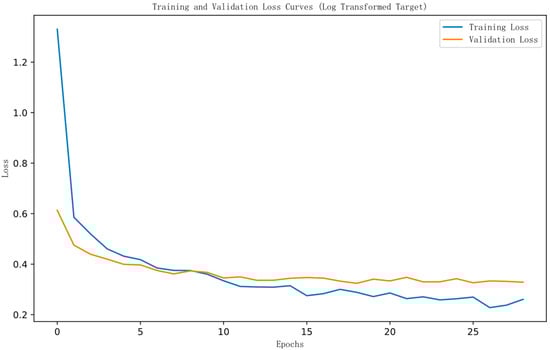
Figure 2.
Training and validation loss of the deep neural network model.
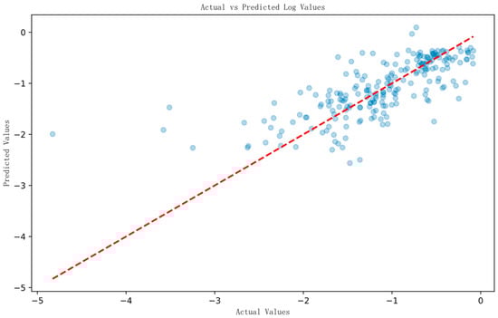
Figure 3.
Scatter plot of predicted vs. actual values of the deep neural network model.
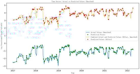
Figure 4.
Time series of the deep neural network model.
Figure 2 illustrates the variations in loss (the value of the loss function) during training and validation as a function of the number of iterations, which serves to evaluate the model’s convergence. Both the training loss and validation loss decrease as the number of iterations increases, indicating that the model is continuously learning and optimizing. In the initial iterations, the training loss declines rapidly, suggesting that the model captures a significant amount of useful information at early stages. After approximately 10 iterations, the loss curve levels off, indicating convergence, whereby further training yields limited improvements. Similarly, the validation loss also decreases rapidly in the early stages, subsequently flattening after about 10 iterations, while remaining slightly higher than the training loss. However, the consistency in both trends suggests that no significant overfitting occurred.
Figure 3 further evaluates the predictive performance of the model by illustrating the relationship between actual values and predicted values derived from the test set. The scatter points representing the actual and predicted values are predominantly clustered around the diagonal line y = x, suggesting a notable degree of consistency between the model’s predictions and the actual outcomes. The distribution of scatter points is relatively uniform on either side of the diagonal, indicating the absence of systematic bias; in other words, there is no significant overestimation or underestimation present. Nevertheless, some outliers are discernible within the scatter plot, with points located farther from the diagonal, highlighting larger prediction errors in specific instances. Additionally, the density of scatter points is greater in the central range of both the horizontal and vertical axes, suggesting that the model’s predictions are more accurate within this range.
Figure 4 provides a visual comparison between actual values and predicted values using a time series plot. The blue solid line represents the smoothed actual values, effectively illustrating the overall trend and fluctuations within the dataset. The green points closely align with the blue solid line, indicating that the smoothing process did not significantly diverge from the original data. The orange dashed line denotes the integration of the smoothed actual values and predicted values, offset to enhance differentiation. The red points signify the predicted values; by comparing these with the green points, one can observe the discrepancies between predicted and actual values. Overall, the trend analysis reveals that the predicted values generally align with the actual values, suggesting that the model effectively captures the primary trends in the data, including instances of social disagreement and investor disagreement.
4.2. The Contagion Mechanism of Social Disagreement to Investor Disagreement
The significant impact of non-economic policy on social divisions indicates that it can indeed shape expectations. The primary distinction between social sentiment and investor sentiment lies in the groups they represent: social sentiment reflects the emotional aggregation of the general public, while investor sentiment specifically pertains to individuals who closely focus on investment-related information.
This section will elucidate the reasons why social disagreements affect investor disagreements, emphasizing that social expectations influence investor expectations. Direct evidence will be presented to highlight the disparities between social disagreements and investor disagreements. Subsequently, a time series graphical analysis will be employed to examine the long-term influence of social sentiments on investor sentiments.
4.2.1. The Contagion Mechanism
The conclusions drawn by Liu et al. (2023) [] indicate that social disagreement and investor disagreement can jointly influence asset pricing; however, the study does not adequately elucidate the mechanisms through which social disagreement impacts investor disagreement.
According to Emotional Contagion Theory, emotions can spread among individuals, particularly in today’s highly interconnected society. The speed and reach of emotional transmission via social networks, media, and other channels have significantly increased (Hatfield et al., 1994) []. Additionally, Bounded Rationality Theory complements this understanding by addressing the behavioral characteristics of investors as they navigate complex information and emotional contagion. This theory posits that due to incomplete information and cognitive limitations, investors are not always able to make optimal decisions; rather, they make choices within the confines of their rationality, rendering them more susceptible to external emotional fluctuations (Simon, 1955) [].
In general, social emotional divergence encompasses broader social information that spreads within large groups through media dissemination, public discussions, and other channels. Given that emotions are highly transmissible and contagious within groups, social emotions gradually exert influence over investor groups. In contemporary society, characterized by frequent information exchange, the pace of this emotional transmission has been markedly accelerated.
According to the above theories, let be defined as the proportion of the population unaffected by emotions in society at time ; as the proportion of the population that has shown emotional divergence at time ; as the rate of emotional transmission at the societal level, which is highly influenced by widespread information; as the proportion of the investor population unaffected by emotions at time ; as the proportion of the investor population showing emotional divergence at time ; as the rate of emotional transmission at the investor level, which is largely influenced by financial information and emotional contagion; and as the recovery rate of emotions (whether in society or among investors).
By drawing from the contagion model, the model for emotional divergence in society can be expressed as follows:
The equation describes how emotional divergence within social groups gradually forms as information spreads widely, and is driven by macro-social factors (policies, social events, etc.). Here, is relatively high because social emotional divergence is influenced by the breadth and diversity of information.
Since investors do not have direct access to all social information, they tend to concentrate on information that is more pertinent to the economic system. Consequently, their investor disagreement tends to lag behind social disagreement, relying on the transmission of social disagreement to their group through the mechanism of emotional contagion. The model of investor disagreement can be expressed as follows:
The equation demonstrates that the propagation rate of investor disagreement, denoted as , is driven by the social disagreement .
To better explain the leading role of social disagreement, the breadth of information is further introduced into the sentiment propagation rate. It is assumed that the propagation rate of social disagreement, , is influenced by the breadth of information, , while the propagation rate of investor disagreement, , depends on the effectiveness of the transmitted information:
Among them, represents the potential breadth of information covered by social disagreement, which is generally larger than (the breadth of market information obtained by investors), as social disagreement covers more diverse information.
The social disagreement is driven by a broad range of potential information and spreads at a faster rate:
Investor disagreement lags behind social disagreement and is transmitted through the contagion of social disagreement:
Because , the spread rate of social disagreement () is faster, while the spread rate of investor disagreement () is slower, leading to the divergence in social disagreement typically preceding the divergence in investor disagreement.
In summary, social disagreement tends to escalate on a larger scale, particularly during extensive policy discussions or significant societal events, where emotional fluctuations become evident. Although investors, as a smaller subgroup, are primarily concentrated on financial markets, they cannot entirely detach themselves from the broader social environment. As social disagreement intensifies, investors perceive these emotional signals through daily social interactions or media exposure, which ultimately influences their market decisions. Due to the lagging effect of information and emotions, social disagreement typically surges in the initial phases of policy implementation or societal events, while investors require additional time to process this external emotional information. Even if investors are not initially attuned to the emotional turmoil instigated by societal events, they start to react to these shifts once such emotions are broadly disseminated into the market via public opinion and news reports.
Moreover, drawing on the theory of bounded rationality, investors’ emotional responses lag behind social disagreement because they need time to analyze and interpret the market signals induced by societal emotions. Particularly when confronted with complex information, investors are unable to adjust their behavior immediately; instead, they are gradually swayed by emotional contagion. Consequently, social disagreement typically precedes investor disagreement, transmitting social-level emotions to the investor group through the mechanism of emotional contagion.
4.2.2. Evidence of Contagion
- (1)
- Data Independence Basis
To investigate and assess the correlation between the two sets of texts, this study integrates two methods for measuring text similarity: cosine similarity and Latent Dirichlet Allocation (LDA) topic model analysis. Cosine similarity quantifies the similarity between two vectors by calculating the cosine of the angle between them, effectively capturing the degree of resemblance between text segments. In this analysis, each document is transformed into a vector weighted by Term Frequency-Inverse Document Frequency (TF-IDF), which reflects the importance of words within the text. The cosine similarity score obtained from these vectors ranges from −1 (completely dissimilar) to 1 (completely similar).
Furthermore, to gain a more nuanced understanding of text correlations, this study employs the LDA topic model. LDA is a statistical model widely used to uncover underlying thematic distributions in extensive textual datasets. Through LDA, each set of texts is decomposed into a series of topics, represented by a set of keywords, allowing for the determination of each document’s topic distribution. Subsequently, the Jensen–Shannon Disagreement (JS disagreement) between the topic distributions of the two text sets is calculated. JS disagreement serves as a measure of the divergence between two probability distributions, providing a quantitative indicator of thematic disagreement.
As illustrated in Table 4, the cosine similarity value between the two text sets is 0.0043. This indicates that while the vectors are closely aligned in the vector space model, the actual similarity between the texts is extremely low, suggesting an almost complete lack of resemblance. Through LDA topic modeling, this study identified five key topics: sustainable living (Topic 1), corporate green development (Topic 2), communication and interaction (Topic 3), new energy vehicles (Topic 4), and market and shareholder relations (Topic 5). These themes range from personal attitudes towards life to corporate strategy and market dynamics, reflecting the richness and multidimensionality of the text data. The JS disagreement value is 0.2652, indicating that while there are differences in thematic distribution between the two text sets, these differences are not highly significant. This result suggests that the texts may share some common points of discussion at the macro-thematic level, yet they exhibit substantial differences in vocabulary, expression, and detail.
Table 4.
Text correlation metrics.
By synthesizing the results from these two methods, we conclude that, although there is some correlation between the two text sets at a macro-thematic level, their similarity in terms of precise wording and expression is quite limited.
- (2)
- Correlation Analysis
This section examines the relationship between social disagreement and investor disagreement, aiming to elucidate the dynamic interaction between the two through quantitative analysis. Given the critical importance of data quality in this study, we adopted the analytical framework proposed by Liu et al. (2023) [] and selected data spanning from 2018 to 2022 for our analysis. This time frame was chosen based on a comprehensive evaluation of the existing literature and the depth of analysis required to accurately capture the evolving dynamics between social sentiment and market responses. Notably, the investor disagreements analyzed here are no longer defined by volatility; instead, they are calculated based on actual verbal sentiment expressed by investors.
Figure 5 illustrates the trends of social disagreement and investor disagreement, employing Gaussian smoothing techniques for data processing. This advanced method not only mitigates random fluctuations but also provides a clearer depiction of the fluctuation patterns between the two forms of disagreement. The analysis reveals that, although social disagreement and investor disagreement exhibit independent fluctuation characteristics in the short term, they demonstrate significant synchronization in long-term trends. Specifically, the sharp declines observed between May and August 2018, the dramatic increase in the first half of 2019, and the rapid decrease in the latter half of 2019 all reflect the close relationship between social and investor sentiment. Following July 2020, this trend became even more pronounced, suggesting that under specific market and societal conditions, a deeper interaction mechanism may exist between social disagreement and investor disagreement.
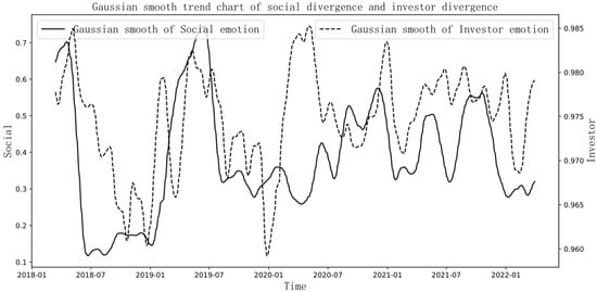
Figure 5.
Trends of social disagreement and investor disagreement.
5. Further Analysis Based on a DSGE Model Incorporating Social Disagreement and Non-Economic Policies
The preceding section demonstrates that non-economic policies, although devoid of intrinsic economic characteristics, can significantly influence economic expectations. This section will investigate how non-economic policies adjust these expectations and affect overall economic dynamics by extending the analytical framework of a dynamic stochastic general equilibrium (DSGE) model.
This paper builds upon the DSGE model presented by Wen (2017) [] by incorporating non-economic policies and social disagreement, representing an advancement of the New Keynesian framework as elaborated in previous research (Woodford, 2003; Smets & Wouters, 2007; Christiano et al., 2005) [,,]. In this model, economic agents comprise numerous households and firms. Households, as labor suppliers, allocate their income towards the consumption of final goods and investment in financial assets, such as bonds and stocks. Firms are categorized into intermediate product firms and final product firms, with the former providing differentiated products to the latter, utilizing labor as an input. Final product firms, owned by households, supply homogeneous goods. Within this framework, intermediate goods markets are characterized by monopolistic competition, whereas the final goods market operates under perfect competition. To ensure wage and price stickiness, the model assumes heterogeneity in the labor supplied by households. Furthermore, to maintain consistency with other assumptions, the conditions regarding capital (Challe & Giannitsarou, 2014) [], the markets for stocks and bonds, the central bank’s monetary policy as represented by the Taylor rule, and the presence of heterogeneous investors (De Grauwe, 2011) [] are aligned with key reference models (Wen Xingchun, 2017) []. Apart from investor expectations, stock price expectations, non-economic policies, and social disagreement, the structure of this model remains consistent with that of a standard DSGE framework. This section will primarily elucidate the key settings that differ from the classical DSGE model, with additional details available in Appendix A.
5.1. Model Setup
5.1.1. Non-Economic Policies
The primary objective of non-economic policies is to mitigate or prevent fluctuations in social disagreement. This implies that non-economic policies are designed to address abnormal fluctuations in social disagreement or anticipated changes stemming from economic policies. To facilitate this, a straightforward linear model is presented for the direct formulation of operational rules governing non-economic policies. This design aligns with the overarching goal of these policies: to reduce fluctuations in social disagreement and to establish unified expectations.
where represents the non-economic policy in period , represents the abnormal fluctuations in social disagreement in period , and represents the central bank’s monetary policy with a time lag of (where ), and are the sensitivity coefficients of non-economic policies to social disagreement and monetary policy shocks. Let represent the average of social disagreement () over the past z periods (z = 20), and thus, , which measures whether there is an abnormal increase in social disagreement.
5.1.2. Behavioral Investors and Social Groups
- (1)
- Social disagreement
Based on the preceding analysis, social disagreement is primarily influenced by non-economic policies and the lag effect of social disagreement rather than by economic policies. In our earlier findings, we identified the lagged autocorrelation of social disagreement across periods 1 to 4 through a VAR model, utilizing the data presented in the previous section. This empirical evidence substantiates the inclusion of these factors in Equation (12).
where are geometrically decaying weights, indicating the influence of the 1- to 4-period lag of social disagreement on current social disagreement. is the coefficient that measures the impact of non-economic policies on social disagreement.
- (2)
- Behavioral Investors
Building upon the findings of Wen (2017) [] and our earlier conclusions (Liu et al., 2023) [], we propose modifications to the behavior of investors. The model continues to classify investors into three categories: optimistic, pessimistic, and fundamental investors (De Grauwe, 2011) []. Optimistic and pessimistic investors are particularly influenced by social disagreement. Previous research (Liu et al., 2023) [] indicates that social disagreement exerts a negative impact on investor sentiment. Specifically, an increase in social disagreement causes emotional investors to perceive an escalation in market risk, consequently diminishing their expectations for stock prices. The expectations regarding stock prices for investors are established as follows:
where is the coefficient of the impact of changes in social disagreement on investor expectations for stock prices. The relationship between and stock price volatility is as follows:
where is the variance in the stock price over the observation period z, is the intercept, and is the sensitivity of forecast disagreement to stock price volatility. indicates that the expectations of emotional investors regarding stock prices are influenced by stock price volatility. Based on our statistical data, the attention of investors and social groups to similar concepts differs, meaning that is not affected by social disagreement.
To model the enduring shifts in emotional investors’ sentiment, we employ a framework rooted in discrete choice theory (Wen, 2017; Anderson et al., 1992; Brock & Hommes, 1997) [,,]. Investors assess the efficacy of three distinct prediction rules in the following manner:
, and represent the variance in the optimistic, pessimistic, and fundamental prediction rules, respectively. are geometrically decaying weights, satisfying , where measures the memory of investors regarding past performance.
Based on the above setup, we can calculate the proportion of each type of investor affected by social disagreement:
Parameter reflects the degree to which investors emphasize the relative performance of prediction rules. When , all investors choose the best-performing prediction rule; when , each rule is chosen by one-third of the investors.
5.1.3. Stock Price Forecast
Beyond the influence of investor disagreement, stock price forecasts are also shaped by social disagreement. As stock price volatility increases, the impact of social disagreement on stock prices becomes more pronounced. Consequently, the model incorporates a new variable: the interaction term between social disagreement and stock price volatility, which serves as a regulatory factor. The specific formulation is presented in Equation (23):
Let represent the average of stock prices () over the past z periods (z = 20), and thus, , which measures whether there is abnormal volatility in stock prices. The absolute value limits the sign change, while the positive and negative changes in indicate the overall sign change of the term.
5.2. Parameter Calibration
The parameter settings of this model are presented in Table 5. The section above the double lines in Table 5 refers to parameter settings derived from previous classical DSGE model research, whereas the section below the double lines outlines the unique settings specific to this model. Notably, the terms ‘Social disagreement’ and ‘Investor disagreement’ are used to denote social and investor discrepancies, respectively.
Table 5.
Parameter calibration table.
5.3. Numerical Simulation
In Wen’s (2017) [] research, the effects of identical monetary policy shocks on stock prices and investor proportions were compared under conditions where equals 0 and 2. The findings revealed that the response mechanism of monetary policy to stock prices can stabilize the proportions of optimistic and fundamental investors, thereby reducing the likelihood of significant fluctuations in the proportion of optimistic investors and facilitating interest rate smoothing. The model results for = 2 are illustrated in Figure 6, which is included here for comparative analysis with the model in this study.
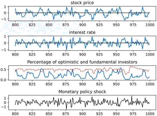
Figure 6.
DSGE model results without social disagreement and non-economic policy in reference article. The red line in the panel 3 graph represents fundamental investors, while the blue line represents optimistic investors.
Furthermore, this paper presents the simulation results of the DSGE model based on the reference model, specifically when the sensitivity coefficient of social disagreement’s impact on non-economic policy () is set to 3, 1.5, 0.5, and −1.5, as illustrated in Figure 7, Figure 8, Figure 9 and Figure 10. A grouped observation reveals that, in Figure 6, Figure 7, Figure 8 and Figure 9, the sensitivity coefficient of social disagreement affecting non-economic policy is positive, while in Figure 10, it is negative. A positive coefficient suggests that non-economic policies effectively mitigate the abnormal growth of social disagreement, whereas a negative coefficient implies that such policies may either permit an increase in social disagreement or exacerbate the situation due to improper implementation.
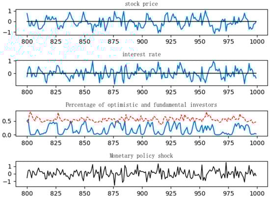
Figure 7.
The red line in the panel 3 graph represents fundamental investors, while the blue line represents optimistic investors.
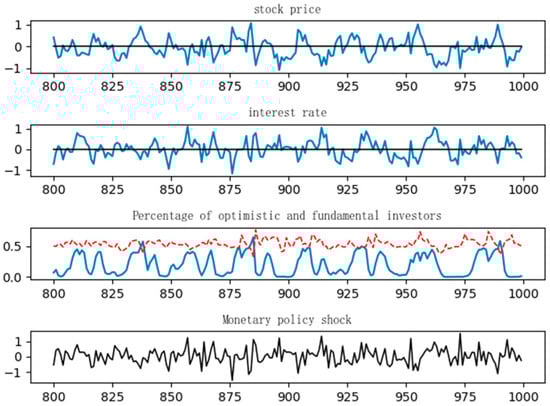
Figure 8.
The red line in the panel 3 graph represents fundamental investors, while the blue line represents optimistic investors.
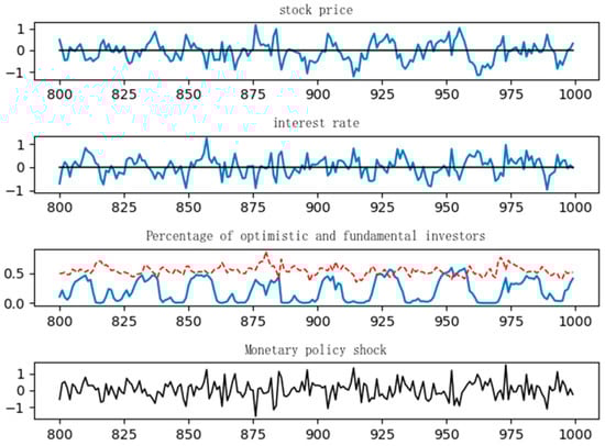
Figure 9.
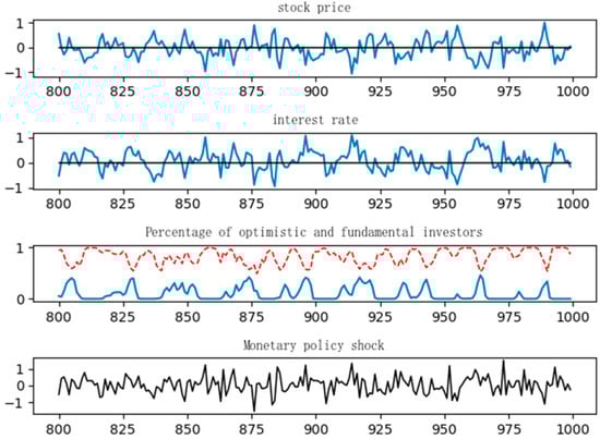
Figure 10.
From the simulation analysis of models characterized by varying coefficient values, the following conclusions can be drawn:
The DSGE model that incorporates social disagreement and non-economic policies produces a more “optimistic” and “symmetrical” distribution of stock prices compared to models that do not account for these variables. As shown in Figure 6, Figure 7, Figure 8, Figure 9 and Figure 10, the system defines a range of intervals based on actual stock values. Figure 6 indicates that the mean stock price is below zero, whereas Figure 7, Figure 8, Figure 9 and Figure 10 illustrate a more symmetrical range of positive and negative stock price fluctuations. This indicates that the DSGE model, which includes social disagreement and non-economic policies, better captures the general pattern of stock price fluctuations around their intrinsic value.
The generalized fluctuations in do not decisively influence stock price movements; rather, they function as a “fine-tuning” mechanism. A larger value of this coefficient correlates with reduced internal disagreement among investors. Figure 7, Figure 8, Figure 9 and Figure 10 explore the variations in stock prices and investor proportions under different levels of . While non-economic policies have minimal impact on the overall trend of stock price changes, they play a crucial role in the finer details. In terms of investor proportions—reflecting investor expectations—non-economic policies exert a significant regulatory effect.
Comparatively, a positive can help reduce stock price volatility to some extent. For instance, Figure 9 and Figure 10 illustrate that the frequency of stock price fluctuations in Figure 10 is significantly higher than that in Figure 9.
These conclusions align with the anticipated outcomes of this research. On the one hand, the introduction of non-economic policies within this model aims to shape economic expectations by controlling and mitigating social disagreement. On the other hand, the role of non-economic policies in macroeconomic management is largely ‘auxiliary’. By harmonizing non-economic and economic policies, the consistency of macroeconomic policy can be enhanced, thereby reducing the negative externalities associated with economic policies.
5.4. Impulse Response Analysis
Additionally, this paper conducts an analysis of the impulse response to a negative monetary policy shock within the DSGE model, utilizing a value of −0.5. Initially, the reference model established by Wen (2017) [] with = 2 was replicated. Unlike the graphs presented in the original article, modifications to led to a notable change in the monetary policy’s response to stock prices, thereby reducing the time required for the model to return to a steady state, as illustrated in Figure 11.
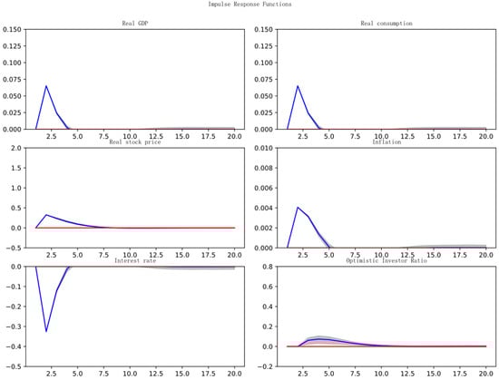
Figure 11.
Impulse response of the DSGE model with in the reference model. The blue line indicates the mean value of the impulse response, while the shaded areas in gray indicate the size of the 5% and 95% quantiles of the impulse response.
In Figure 12, under the adverse effects of monetary policy (which serves as a positive economic stimulus), GDP, consumption, stock prices, inflation, and the proportion of optimistic investors all exhibited positive growth, while interest rates experienced a decline. The mean, 5th percentile, and 95th percentile impulse response values of the macroeconomic variables displayed no significant differences or only weak distinctions; however, investor disagreement showed marked variation among these three metrics. This suggests that in the reference model, the shock from monetary policy introduces greater uncertainty into the stock market, while the uncertainty surrounding macroeconomic variables remains comparatively lower.
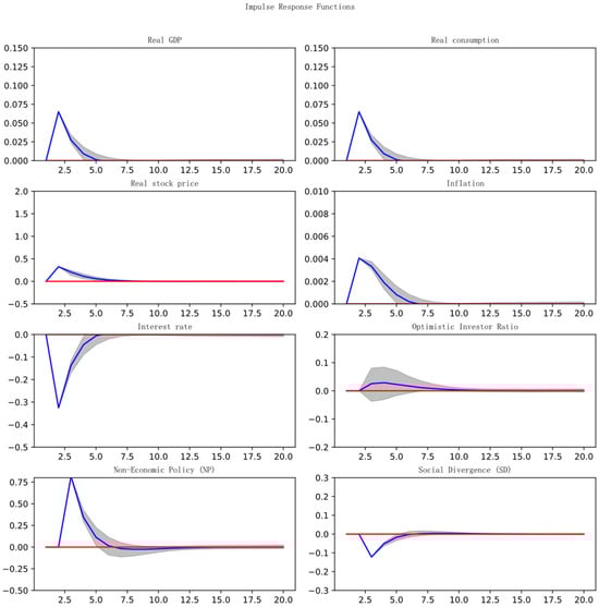
Figure 12.
Impulse response of the DSGE model with . The blue line indicates the mean value of the impulse response, while the shaded areas in gray indicate the size of the 5% and 95% quantiles of the impulse response.
In the modified model presented in this study, the conclusions derived from the original model underwent significant alterations, as illustrated in Figure 12. In this figure, = −2.5 indicates that under an active monetary policy (characterized by lower interest rates), the implementation of active non-economic policies mitigates social disagreement, thereby enhancing the effectiveness of monetary policy.
The distinctions between Figure 11 and Figure 12 can be summarized as follows: First, the uncertainty associated with macroeconomic variables, in response to monetary policy, increased, aligning more closely with real-world conditions. Second, all variables exhibited prolonged durations in returning to equilibrium. This extended timeframe highlights the challenges posed by social disagreement (irrational factors), making it more difficult for the macroeconomy to attain equilibrium, which is a more accurate reflection of reality. Furthermore, this suggests that the economic stimulus effects of monetary policy are prolonged, thereby amplifying the impact of such policies. Third, in the context of stimulating the economy through monetary policy, non-economic policies—while keeping other economic objectives constant—reduce the proportion of optimistic investors and elevate stock prices. This, in turn, increases the share of fundamental investors, decreases the proportion of pessimistic investors, and diminishes social disagreement.
Similarly, Figure 13 analyzes the impulse response when is positive. In this context, a positive signifies the implementation of conservative non-economic policies, thereby allowing active monetary policy to function independently. The figure illustrates that while the proportion of optimistic investors increases, this does not result in a significant enhancement in the absolute effects of other economic variables. Rather, it reduces the duration of the active monetary policy stimulus, which ultimately extends the period of inflation.
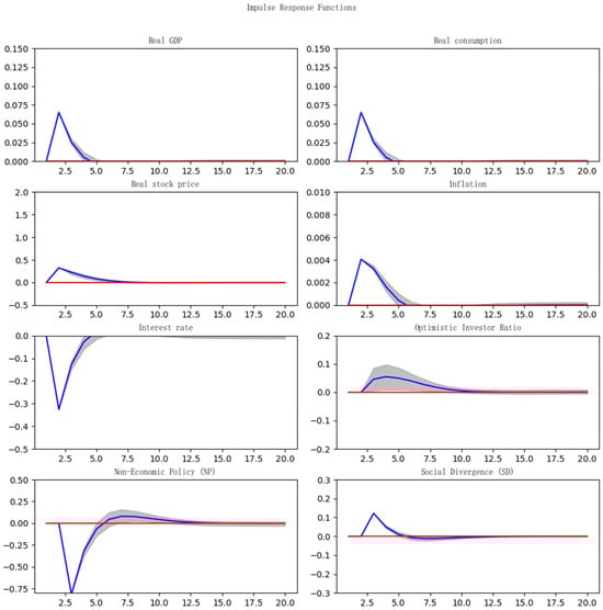
Figure 13.
Impulse response of the DSGE model with . The blue line indicates the mean value of the impulse response, while the shaded areas in gray indicate the size of the 5% and 95% quantiles of the impulse response.
6. Suggestions and Conclusions
6.1. Policy Analysis and Suggestions
Based on the analysis presented above, it is clear that non-economic policies have the potential to manage divisions in social sentiment effectively. The role of these policies in addressing social sentiment divisions should focus on long-term governance strategies. The following specific policy recommendations are proposed:
- (1)
- Prioritize the Publication of Central Regulations
Analysis: In China, central government policies typically carry greater authority and enforcement power. For example, resolutions from the National Congress of the Communist Party of China are generally elevated to national laws during the National People’s Congress and are disseminated across government agencies, educational institutions, and state-owned enterprises. Research findings indicate that central regulations can significantly reduce social disagreements by providing clear policy directions and implementation standards. Therefore, it is advisable to increase both the frequency and strength of central regulations’ publication to enhance the consistency of local government implementation. This approach will help mitigate social disagreements arising from varying local interpretations, thereby ensuring more effective achievement of policy objectives.
- (2)
- Optimize Administrative Approval Processes
Analysis: Administrative approval processes are often seen as significant obstacles to economic and social development in China. For instance, the IPO registration system for the main board market was only officially implemented in 2023, underscoring the complexities associated with these processes. Such cumbersome procedures may lead to public resentment towards policies. It is therefore recommended to streamline the approval steps across various departments and implement the “once only” reform to enhance administrative efficiency, thus reducing social disputes and public dissatisfaction stemming from approval processes.
- (3)
- Promote Interdepartmental Collaboration
Analysis: Research indicates that effective collaboration among different departments can reduce social disagreements, while a lack of cooperation may exacerbate social tensions. In China, policies often involve multiple departments, and the absence of effective communication and coordination mechanisms can hinder successful policy implementation. It is recommended to establish a cross-departmental joint meeting mechanism, based on empirical evidence, that assigns and designates optimal “departmental partners” for collaboration. This will enhance policy communication and ensure that all departments maintain a consistent understanding and execution of policies, thereby reducing uncertainty and conflicts during the implementation process.
- (4)
- Monitor and Evaluate Policy Interaction Effects
Analysis: As the policy environment becomes increasingly complex, understanding the interactions between policies grows in importance. China should establish a dynamic policy monitoring and evaluation mechanism that regularly analyzes the synergies and conflicts between non-economic and economic policies, taking into account fluctuations in social sentiments. This will facilitate timely policy adjustments, enhancing both adaptability and effectiveness, thus reducing the likelihood of social disagreements.
6.2. Conclusions
This study offers a comprehensive examination of the systematic integration of non-economic policies into the framework for assessing macroeconomic coherence, with a particular emphasis on green policies. The findings highlight the vital role that non-economic policies play in managing social disagreement, shaping investor expectations, and ultimately enhancing the consistency and effectiveness of macroeconomic policy interventions. Through a combination of empirical analysis and a Dynamic Stochastic General Equilibrium (DSGE) model, several key conclusions have been drawn.
First, while non-economic policies may not directly influence economic activities, they significantly impact social sentiment, effectively reducing social disagreement and exerting a long-term influence on investor expectations. This was evidenced by the construction of a social sentiment index utilizing large-scale web-scraped data, which revealed that an increase in the issuance of policy measures leads to a substantial reduction in social disagreement, thereby fostering more favorable market expectations.
Second, by integrating non-economic policies into the DSGE model, this study provides theoretical validation of the potential for these policies to contribute to macroeconomic regulation. The results indicate that the dynamic relationship between social disagreement and investor disagreement can be modulated through the strategic implementation of non-economic policies, which, in turn, enhances the efficacy of economic policies. Simulation and impulse response analysis further demonstrate that non-economic policies can extend the positive effects of economic interventions, thereby making policy measures more sustainable over time.
The innovative contribution of this research lies in its introduction of a novel conceptual framework that integrates “non-economic policies—social disagreement—investor expectations” into the macroeconomic coherence paradigm. This study not only provides empirical evidence for the tangible economic impacts of non-economic policies through the management of sentiment and expectations but also offers theoretical insights to guide policymakers in aligning non-economic and economic policy efforts. By embedding these insights into a more realistic policy model, this research presents actionable recommendations for the formulation and implementation of future policies, particularly in areas such as environmental protection, where public sentiment plays a crucial role. The strategic use of non-economic policies can therefore be instrumental in enhancing the quality of economic growth and managing market expectations.
In conclusion, this research elucidates a clear path forward for policymakers, demonstrating that in today’s complex economic landscape, non-economic policies can serve as an effective complement to traditional economic measures. It also paves the way for new academic inquiry into the interplay between macroeconomic policies and non-economic factors. Future research could build on these findings by exploring the effects of different types of non-economic policies across various economic sectors, thereby enriching both the theoretical framework and practical applications of macroeconomic policy.
Author Contributions
Conceptualization, J.L. and J.M.; methodology, J.L.; software, J.L.; validation, J.L., J.M. and Y.T.; formal analysis, J.L. and Y.T.; investigation, J.L.; resources, J.M.; data curation, J.M.; writing—original draft preparation, J.L.; writing—review and editing, Y.T.; visualization, J.L.; supervision, J.M.; project administration, J.M.; funding acquisition, J.M. All authors have read and agreed to the published version of the manuscript.
Funding
This research was funded by [72101009] grant number [National Natural Science Foundation of China] And The APC was funded by [Junjun Ma].
Data Availability Statement
Research data for this article can be requested from the corresponding author.
Conflicts of Interest
The authors declare no conflict of interest.
Appendix A
- (I)
- Household
- (1)
- Consumption, Income, and Expenditure
In line with the classical DSGE framework, the utility of households is derived from consumption, labor supply, and a discount factor:
The specific form of is given by Equation (A2):
Here, and represent, respectively, the intertemporal elasticity of substitution in consumption and the elasticity of labor supply with respect to wages. In accordance with the classical DSGE setup, the household budget constraint can be expressed as follows:
On the left-hand side of this equation, we account for household consumption and investments in stocks and bonds. On the right-hand side, various income sources and asset holdings are considered, including bond interest income, labor wages, previous period stock holdings, and dividend payments. By combining equations (A1) and (A2) with the budget constraint (A3) and constructing the corresponding Lagrangian, the utility maximization conditions can be derived as in Equations (A4)–(A6):
From these conditions, the Euler equations are derived as follows:
- (2)
- Labor Supply with Wage Stickiness
In the classical DSGE model, as illustrated by Equation (A9), the labor supplied by household is a function of the average labor supply level (), the relative wage () and the elasticity of substitution in labor (). In this paper, it is assumed that households do not immediately adjust their wage levels to optimal levels when supplying labor to the production sector. A proportion of households cannot adjust their wage to the optimal level , and their actual wage is determined as follows:
When making decisions about consumption and labor, households must balance current consumption, future consumption, and labor supply. As shown in Equation (A11), the utility derived from future consumption and the difference between current labor income and future consumption must be considered:
The labor supply curve, representing the relationship between labor supply and wages, is as follows:
where .
Substitute the constraint Equation (A8) into Equation (A7) and apply the first-order maximization condition with respect to to obtain:
Additionally, since each household that can adjust to the optimal wage level is homogeneous, the subscript can be removed. Based on the setting for the proportion of households that can adjust to the optimal wage and the wage setting, Equation (A14) is obtained, which represents the aggregate wage level:
Finally, by eliminating , the real wage Equation (A15) can be derived, where “^” indicates the deviation from the steady state:
where ; ; .
- (II)
- Production Sector
In this paper, the final goods market is perfectly competitive, while the intermediate goods market is monopolistically competitive. The input for final goods firms comes from intermediate products, meaning that the inputs among the final goods firms are not perfectly substitutable.
- (1)
- Final Goods Firms
The production function for final goods firms is as follows:
where is the elasticity of substitution between different types of intermediate goods, and is the demand for the intermediate product at time . Specifically, is expressed as shown in Equation (A17):
where is the price of the final goods, and is the price of the intermediate goods.
- (2)
- Intermediate Goods Firms
The production function of intermediate goods firms is as follows:
where reflects total factor productivity (technology). Accordingly, the inverse function of labor input is as follows:
And the marginal cost is as follows:
Based on the production function of intermediate firms, the first-order derivative with respect to labor is as follows:
Substituting Equation (A21) into Equation (A20), we obtain:
The real marginal cost requires adjusting Equation (A22) for the price level:
The profit function of intermediate firms is as follows:
The profit margin is as follows:
Since monopoly profits are distributed as dividends to the firm owners (residents), the dividend is as follows:
- (3)
- Price Setting for Intermediate Firms
According to the setup, the products produced by intermediate firms are heterogeneous, and the market is monopolistically competitive. Referring to Smets & Wouters (2003) [], Christiano et al. (2005) [], and Calvo (1983) [], the price adjustment for intermediate firms is limited, with a proportion of firms unable to adjust to the optimal price, while the remaining firms can adjust to the optimal price. The actual price setting for firms unable to adjust to the optimal price is as follows:
Then, the overall price equation is as follows:
Additionally, the optimization problem faced by intermediate firms that can adjust to the optimal price is shown in Equation (A29). In this case, represents the revenue of such firms, represents the cost component, and is the marginal utility of the actual income of intermediate firms at time .
The constraint of this optimization problem is as follows:
Further, based on Equation (A29) and the constraint Equation (A30), constructing a Lagrange function and solving the first-order maximization problem yields the following:
Since every intermediate firm of this type faces the same optimal price, the subscript can be removed. Combining the overall price Equation (A28) with Equation (A31), performing log-linearization, and eliminating , the Phillips Curve is obtained:
where:
- (III)
- Government Sector
Central Bank Monetary Policy:
Following Woodford (2003), the extended Taylor rule is adopted as the guideline for central bank monetary policy:
where is the interest-rate-smoothing coefficient, representing the degree to which the central bank depends on past interest rates when adjusting the nominal interest rate. and are the response coefficients of the nominal interest rate to the output gap, inflation gap, and stock price gap, respectively.
References
- Sharpe, W.F. Capital asset prices: A theory of market equilibrium under conditions of risk. J. Financ. 1964, 19, 425–442. [Google Scholar]
- Hong, H.; Stein, J.C. Disagreement and the stock market. J. Econ. Perspect. 2007, 21, 109–128. [Google Scholar] [CrossRef]
- Zhang, S. Preferences, Beliefs, Information, and Securities Prices; Shanghai People’s Publishing House: Shanghai, China, 2002. (In Chinese) [Google Scholar]
- Wu, H. Heterogeneous Interpretations, Overconfidence, and Market Reactions to Public Information: A Study Based on the Perspective of Investor Sentiment Disparities. Investig. Res. 2022, 41, 91–112. (In Chinese) [Google Scholar]
- Giacomini, R.; Skreta, V.; Teles, P. Heterogeneity, Inattention and Bayesian Updates. Am. Econ. J. Macroecon. 2020, 12, 282–309. [Google Scholar] [CrossRef]
- Kim, J.S.; Ryu, D.; Seo, S.W. Investor sentiment and return predictability of disagreement. J. Bank. Financ. 2014, 42, 166–178. [Google Scholar] [CrossRef]
- Shi, Y.; Li, F. Short Selling Restrictions, Convergence of Opinions, and the Price Effect of Information Disclosure: Empirical Evidence from the A-Share Market. Financ. Res. 2012, 08, 111–124. (In Chinese) [Google Scholar]
- Liu, Y.; Zhu, H. Individual and Institutional Investors: Who Influences A-Share Price Changes? A Perspective Based on Heterogeneous Beliefs of Investors. Chin. Manag. Sci. 2018, 26, 120–130. (In Chinese) [Google Scholar]
- Jiang, H.; Sun, Z. Dispersion in beliefs among active mutual funds and the cross-section of stock returns. J. Financ. Econ. 2014, 114, 341–365. [Google Scholar] [CrossRef]
- Cookson, J.A.; Niessner, M. Why Don’t We Agree? Evidence from a Social Network of Investors. J. Financ. 2020, 75, 173–228. [Google Scholar] [CrossRef]
- Wang, X.; Xiang, Z.; Xu, W.; Yuan, P. The causal relationship between social media sentiment and stock return: Experimental evidence from an online message forum. Econ. Lett. 2022, 216, 32–76. [Google Scholar] [CrossRef]
- Sanford, A. Does Perception Matter in Asset Pricing? Modeling Volatility Jumps Using Twitter-Based Sentiment Indices. J. Behav. Financ. 2022, 23, 262–280. [Google Scholar] [CrossRef]
- Liu, T.; Liu, J.; Ma, J.; Tai, Y. Uncovering the hidden impact: Noninvestor disagreement and its role in asset pricing. J. Risk 2023, 25, 25–52. [Google Scholar] [CrossRef]
- Friedman, M. The role of monetary policy American Economic Review (1968) 58, March, pp. 1–17. In A Macroeconomics Reader; Routledge: London, UK, 1997. [Google Scholar]
- Mankiw, N.G.; Romer, D.; Weil, D.N. A Contribution to the Empirics of Economic Growth. Q. J. Econ. 1992, 107, 407–437. [Google Scholar] [CrossRef]
- Kydland, F.E.; Prescott, E.C. Rules Rather Than Discretion: The Inconsistency of Optimal Plans. J. Political Econ. 1977, 85, 473–491. [Google Scholar] [CrossRef]
- Liu, T.; Chen, X.; Liu, J. Economic Policy Uncertainty and Enterprise Financing Efficiency: Evidence from China. Sustainability 2023, 15, 8847. [Google Scholar] [CrossRef]
- Chen, Y. The Connotation and Implementation of Demand-Side Management: The Perspective of "Three-in-One" Macro Policy. Social Sciences in Chinese Higher Education. Institutions 2021, 6, 94–100. (In Chinese) [Google Scholar]
- Zhang, J. Exploring the Construction of a New System and Direction for Macroeconomic Regulation Policies with Chinese Characteristics. J. Xiangtan Univ. (Philos. Soc. Sci. Ed.) 2023, 47, 97–106. (In Chinese) [Google Scholar]
- Azariadis, C. Self-fulfilling prophecies. J. Econ. Theory 1981, 25, 380–396. [Google Scholar] [CrossRef]
- Farmer, R.E.; Guo, J.T. Real business cycles and the animal spirits hypothesis. J. Econ. Theory 1994, 63, 42–72. [Google Scholar] [CrossRef]
- Benhabib, J.; Farmer, R.E. Indeterminacy and increasing returns. J. Econ. Theory 1994, 63, 19–41. [Google Scholar] [CrossRef]
- Sargent, P.B. The diversity of neuronal nicotinic acetylcholine receptors. Annu. Rev. Neurosci. 1993, 16, 403–443. [Google Scholar] [CrossRef] [PubMed]
- De Grauwe, P. Animal spirits and monetary policy. Econ. Theory 2011, 47, 423–457. [Google Scholar] [CrossRef]
- Wen, X. Investor Sentiment, Monetary Policy Adjustment and Stock Market Boom-bust Cycles: Based on a Heterogeneous Expectation Stock Market DSGE Model. J. Cent. Univ. Financ. Econ. 2017, 08, 23–36+46. (In Chinese) [Google Scholar]
- Liu, C.C.; Liang, X.D.; Jiang, W. Research on Chinese Entrepreneur Confidence, Investor Confidence and Macroeconomic Fluctuation under DSGE Framework. J. Qingdao Univ. (Nat. Sci. Ed.) 2023, 36, 116–123+130. (In Chinese) [Google Scholar]
- Antweiler, W.; Frank, M.Z. Is all that talk just noise? The information content of internet stock message boards. J. Financ. 2004, 59, 1259–1294. [Google Scholar] [CrossRef]
- Hatfield, E.; Cacioppo, J.T.; Rapson, R.L. Emotional Contagion; Cambridge University Press: Cambridge, UK, 1994. [Google Scholar] [CrossRef]
- Simon, H.A. A behavioral model of rational choice. Q. J. Econ. 1955, 69, 99–118. [Google Scholar] [CrossRef]
- Woodford, M. Optimal interest-rate smoothing. Rev. Econ. Stud. 2003, 70, 861–886. [Google Scholar] [CrossRef]
- Smets, F.; Wouters, R. Shocks and frictions in US business cycles: A Bayesian DSGE approach. Am. Econ. Rev. 2007, 97, 586–606. [Google Scholar] [CrossRef]
- Christiano, L.J.; Eichenbaum, M.; Evans, C.L. Nominal rigidities and the dynamic effects of a shock to monetary policy. J. Political Econ. 2005, 113, 1–45. [Google Scholar] [CrossRef]
- Challe, E.; Giannitsarou, C. Stock prices and monetary policy shocks: A general equilibrium approach. J. Econ. Dyn. Control 2014, 40, 46–66. [Google Scholar] [CrossRef]
- Anderson, S.P.; De Palma, A.; Thisse, J.F. Discrete Choice Theory of Product Differentiation; MIT Press: Cambridge, MA, USA, 1992. [Google Scholar]
- Brock, W.A.; Hommes, C.H. A rational route to randomness. Econom. J. Econom. Soc. 1997, 65, 1059–1095. [Google Scholar] [CrossRef]
- Castelnuovo, E.; Nistico, S. Stock market conditions and monetary policy in a DSGE model for the US. J. Econ. Dyn. Control 2010, 34, 1700–1731. [Google Scholar] [CrossRef]
- Nisticò, S. Monetary policy and stock-price dynamics in a DSGE framework. J. Macroecon. 2012, 34, 126–146. [Google Scholar] [CrossRef]
- Bofinger, P.; Debes, S.; Gareis, J.; Mayer, E. Monetary policy transmission in a model with animal spirits and house price booms and busts. J. Econ. Dyn. Control 2013, 37, 2862–2881. [Google Scholar] [CrossRef]
- Mei, D.; Gong, L. Currency Mismatch, Revaluation and Output Fluctuations. Quant. Econ. Tech. Econ. Res. 2011, 28, 37–51. [Google Scholar]
- Smets, F.; Wouters, R. An estimated dynamic stochastic general equilibrium model of the euro area. J. Eur. Econ. Assoc. 2003, 1, 1123–1175. [Google Scholar] [CrossRef]
- Calvo, G.A. Staggered prices in a utility-maximizing framework. J. Monet. Econ. 1983, 12, 383–398. [Google Scholar] [CrossRef]
Disclaimer/Publisher’s Note: The statements, opinions and data contained in all publications are solely those of the individual author(s) and contributor(s) and not of MDPI and/or the editor(s). MDPI and/or the editor(s) disclaim responsibility for any injury to people or property resulting from any ideas, methods, instructions or products referred to in the content. |
© 2024 by the authors. Licensee MDPI, Basel, Switzerland. This article is an open access article distributed under the terms and conditions of the Creative Commons Attribution (CC BY) license (https://creativecommons.org/licenses/by/4.0/).