Adjacency List Algorithm for Traffic Light Control Systems in Urban Networks

Abstract

The increasing complexity of urban road networks has driven the development of Intelligent Transportation Systems (ITS) to optimize vehicle flow. To address this challenge, this paper presents an algorithm and MATLAB function that generates an adjacency list of traffic signals to provide detailed information about the relationships between all signals within a network. This list is based on stable structural road and traffic lights data and offers a crucial global perspective for signal coordination, especially in managing multiple intersections. An adjacency list is more efficient than matrices in terms of space and computational cost, allowing for the identification of critical signals before applying advanced optimization techniques such as neural networks or hypergraphs. We successfully tested the proposed method on three networks of varying complexity extracted from VISSIM and VISUM, demonstrating its effectiveness even in networks with up to 8372 links and 547 traffic lights. This tool provides a solid foundation for improving urban traffic management and coordinating signals across intersections.

1. Introduction

Urban road networks are becoming increasingly complex, and the demand for mobility is on the rise. This has led to the development of smart traffic management systems. These systems leverage cutting edge technologies such as artificial intelligence, machine learning, and IoT to improve road safety, ease congestion, and reduce pollution in our cities [1].

To effectively optimize traffic lights, it is necessary to identify critical signals in advance. This allows for targeted improvements in traffic flow. Typically, current optimization techniques rely on timing data from intersection controllers [2] or information from external sensors [3]. Strategies for managing multiple intersections also require data on how these intersections relate to each other [4]. However, databases with traffic signal timing are generally scarce, regardless of the network type. Furthermore, the frequent adjustments required pose a challenge in keeping timing data up-to-date.

In this paper, we present a novel approach for identifying critical traffic signals within a road network before implementing specific optimization techniques. By determining critical signals early on, we can focus our optimization strategies on key areas of the network. This structural insight is particularly valuable when managing complex networks, analyzing multiple intersections, or using computationally intensive methods such as deep learning or reinforcement learning.

Our approach is designed to work well with a wide range of advanced optimization and prediction techniques. It systematically prioritizes signal analysis based on network topology. Essentially, it acts as a filter that directs computational resources to the most crucial points, thereby enhancing overall system efficiency.

Fortunately, we have access to numerous databases that provide detailed and stable information on road topology and infrastructure. These include regional databases such as PeMS, METR-LA [5], and FHWA [6] as well as global sources such as OpenStreetMap and GeoFabrik [7]. These databases cover large areas and contain stable information, as changes in road infrastructure occur infrequently, making them reliable for deriving the stable relationships necessary for effective traffic management.

This work aligns with and complements advanced traffic control approaches such as STMARL (Spatio-Temporal Multi-Agent Reinforcement Learning) [8]. While STMARL focuses on reinforcement learning to control multiple traffic lights in a coordinated manner, our method provides the structural foundation necessary for such approaches. The adjacency list that we generate can serve as direct input for the Graph Neural Network (GNN) models used in STMARL, thereby facilitating the representation of spatial relationships between traffic lights.

We use an adjacency matrix of traffic signals in the network to represents all relationships between signals and allow for on-demand access. To generate this matrix more efficiently, we use robust and stable data on road infrastructure and signal locations. Although an adjacency matrix is traditionally used for this purpose, we prefer an adjacency list. An adjacency list represent node connections through tuples, which are more computationally efficient in reducing memory usage and processing time [9].

The adjacency matrix or list can be applied across various network topologies, and only requires updating when infrastructure changes occur. This makes it a sustainable long-term tool for use in traffic light management systems.

The adjacency list of traffic lights provides essential information for traffic coordination strategies. By identifying which traffic lights are connected and how they relate to each other within the network, traffic engineers are better able to plan signal coordination and implement green wave strategies. Green waves, where consecutive traffic lights along a route turn green in sequence to allow for continuous traffic flow, require precise knowledge of which traffic lights are connected and their spatial relationships. This structural information is particularly valuable in complex urban networks, where multiple potential routes may exist and the optimal coordination patterns may not be immediately apparent.

In addition to using the adjacency list as a prefilter for critical signals, the information it provides is highly valuable for use in advanced optimization techniques such as Graph Neural Networks (GNNs). GNNs leverage adjacency matrices to propagate information, thereby enhancing model capacity to predict traffic flow [10]. However, most GNN-based approaches focus on node interactions between roads or intersections and do not explicitly considering traffic signal interactions, due in part to limited data describing their mutual influence.

Furthermore, information about traffic signal relationships can be valuable in analyzing road networks through hypergraphs. Hypergraphs allow for simultaneous modeling of different sets of relationships, including those between intersections, roads, and signal interactions, offering an improved representation of complex relationships in road networks [11,12].

Despite these advancements, no existing databases or algorithms establish such a comprehensive relationship map for traffic signals using widely available data sources. This paper proposes an algorithm and a MATLAB function (called Adjacency_list_of_signal_heads) which generates an adjacency list of traffic lights to provide detailed information on relationships among all traffic lights in a road network. This information provides a global perspective on signal interactions, which is critical for optimizing coordination and synchronization.

In summary, this work presents the following key contributions:

• A novel approach for identifying critical traffic signals within a road network prior to implementing optimization techniques, providing a structural perspective on signal relationships.
• An efficient algorithm and MATLAB function called Adjacency_list_of_signal_heads that generates comprehensive adjacency lists of traffic lights, detailing their relationships within the network.
• A systematic framework for integrating the structural information from the adjacency lists into existing traffic prediction and dynamic control techniques for enhanced traffic light coordination and synchronization.
• A foundation for planning traffic light coordination strategies such as green waves by providing detailed knowledge of the structural relationships between traffic lights.
• A scalable and adaptable method that can accommodate different network topologies and only requires updates when infrastructure changes occur, making it a sustainable tool for long-term traffic management systems.
• Proposals for how traffic light relationship data can be leveraged in advanced modeling techniques such as graph neural networks and hypergraphs to improve the representation and optimization of complex urban traffic networks.

The rest of this paper is organized as follows: Section 2 reviews related work in traffic signal optimization and control methods; Section 3 provides key definitions and concepts used throughout the paper; Section 4 describes the materials and methods, including the proposed algorithm and the methodology for generating the adjacency list of traffic signals; Section 5 present complementary codes that support our approach; Section 6 discusses the results of our experiments, highlighting the effectiveness of our approach; Section 7 provides a discussion of our findings and their implications; finally, Section 8 concludes the paper and suggests directions for future research.

2. Related Works

The optimization of traffic light control systems has been a subject of intense research in recent years, driven by the increasing challenges of urban congestion and the need for more efficient transportation networks. This section provides an overview of key approaches and methodologies that have been developed to address these challenges. We begin by examining the Spatio-Temporal Multi-Agent Reinforcement Learning (STMARL) framework, which represents a significant advancement in coordinated traffic light control. Following this, we explore GPS-based methods for identifying and locating traffic signal controllers, highlighting both their strengths and limitations. Finally, we delve into the emerging field of hypergraph-based approaches for traffic forecasting. Throughout this review, we draw comparisons to our proposed adjacency list/matrix method, emphasizing how our approach complements, extends, or differs from these existing methodologies in the context of traffic light management and optimization.

2.1. STMARL: Spatio-Temporal Multi-Agent Reinforcement Learning

Wang et al. [8] proposed STMARL, a framework designed to optimize traffic light control by capturing the spatiotemporal dependencies among multiple traffic lights. The key components of STMARL include:

• A directional traffic light adjacency graph representing spatial relationships between intersections.
• Integration of historical and current traffic data using Recurrent Neural Networks (RNNs).
• A Graph Neural Network (GNN) with an attention mechanism to model relationships among multiple traffic lights.
• Distributed decision-making using deep Q-learning for coordinated control across multiple intersections.

STMARL addresses challenges such as the exponential growth of the action space with increasing agents and the difficulty of formulating coordination among multiple traffic lights. The framework’s effectiveness has been demonstrated through experiments on both synthetic and real-world datasets.

While STMARL offers a sophisticated approach to traffic light control, our proposed method of using adjacency lists provides several advantages:

• Computational efficiency: Our approach is less computationally intensive, especially for large networks.
• Independence from historical data: Unlike STMARL, our method primarily relies on network topology, making it more robust to changes in traffic patterns.
• Scalability: Our method can be easily applied to networks of any size without a significant increase in computational complexity.
• Flexibility: Our approach can serve as a foundation for various optimization methods, and is not limited to reinforcement learning.
• Reduced sensor dependency: STMARL requires a network of sensors for real-time traffic data, while our method can function with static road network information.

While STMARL and other GNN-based approaches offer sophisticated solutions for traffic light control, they rely heavily on complex data structures and real-time information. Our adjacency list/matrix method provides a fundamental structural representation that could significantly enhance these approaches. By offering a clear, efficient, and stable representation of the traffic network topology, our method can serve as a crucial preprocessing step for STMARL and similar GNN-based systems. It reduces the computational overhead of constructing and updating the network structure in real-time, allowing these advanced algorithms to focus on optimizing traffic flow rather than constantly reassessing network topology. Moreover, the scalability and low computational cost of our approach make it an ideal foundation for expanding STMARL and other GNN methods to larger and more complex urban environments. In essence, while STMARL and related approaches excel in dynamic optimization, our method provides the stable structural backbone upon which these sophisticated systems can build, potentially improving their efficiency and applicability in real-world scenarios.

2.2. Identification of Intersection Controllers

Vlachogiannis et al. [13] explored the use of GPS data to identify and locate traffic signal controllers at intersections. Their method involves the following steps:

• Collecting GPS trajectories from vehicles.
• Identifying stop points along these trajectories.
• Clustering stop points to identify potential intersections.
• Analyzing the temporal distribution of stops to distinguish between signalized and non-signalized intersections.
• Using a machine learning algorithm to classify intersections and determine the presence of traffic signals.

While this GPS-based approach offers some advantages, such as the ability to detect changes in traffic signal infrastructure and identify temporary signals, our adjacency list method provides several distinct benefits:

• Independence from real-time data: Unlike the GPS method, which relies on continuous data collection from vehicles, our approach uses static road network information, which makes it more stable and less prone to short-term fluctuations in traffic patterns.
• Comprehensive network view: Our method provides a complete structural representation of the entire traffic light network, rather than focusing on individual intersections as the GPS method does.
• Lower implementation cost: The GPS approach requires access to large amounts of vehicle trajectory data, which may be costly or difficult to obtain. Our method can be implemented using existing road network data, reducing dependency on external data sources.
• Privacy preservation: By not relying on individual vehicle data, our approach avoids potential privacy concerns associated with tracking vehicle movements.
• Scalability: Our adjacency list method can be easily scaled to very large road networks without significantly increasing computational complexity, whereas the GPS method may face scaling challenges due to the increasing volume of trajectory data.
• Predictive capability: The structural information provided by our method can be used to predict the impact of changes in the network, such as the addition or removal of traffic lights, which is not directly possible with the GPS-based approach.

While the GPS-based method excels in detecting real-time changes and temporary signals, our adjacency list approach provides a more stable, comprehensive, and scalable foundation for traffic light management systems that is particularly well suited for long-term planning and network-wide optimization strategies.

2.3. Hypergraph-Based Approaches for Traffic Analysis

Recent advancements in traffic flow analysis have seen the emergence of hypergraph-based methods, which offer a more comprehensive representation of complex road network relationships. A notable example is the work by Luo et al. [11], who proposed a directed hypergraph attention network for traffic forecasting. This approach leverages the power of directed hypergraphs to capture multidimensional and directional relationships within traffic networks.

Their method includes:

• Construction of a directed hypergraph that represents both spatial and temporal dependencies in the road network to account for the directionality of traffic flow.
• A novel directed hypergraph attention network (DHGAT) that learns to aggregate information from relevant neighboring roads considering the direction of traffic flow.
• Integration of both short-term and long-term temporal dependencies through a combination of graph attention mechanisms and Gated Recurrent Units (GRUs).

This directed hypergraph-based approach demonstrates several advantages over traditional methods:

• Enhanced representation of complex intersections and traffic patterns, including the directionality of traffic flow.
• Improved capture of nonlinear relationships in traffic flow.
• Better handling of spatial heterogeneity and temporal dynamics in urban road networks.

While the work of Luo et al. focuses on traffic flow forecasting, the concept of using directed hypergraphs to represent road networks aligns well with our adjacency list/matrix approach. Our method could potentially be extended to incorporate directed hypergraph structures, allowing for a more detailed representation of complex intersections and their relationships, such as the directionality of traffic flow. This could lead to more accurate and comprehensive traffic light control strategies, especially in urban areas with intricate road layouts and complex traffic patterns.

Additionally, research on hypergraph convolutions applied to traffic management suggests that these models can not only represent relationships between main nodes (such as intersections and roads) but also integrate data about traffic lights to enhance synchronization and reduce congestion [12].

Moreover, the integration of hypergraph-based representations with our adjacency list/matrix could provide a foundation for more sophisticated traffic optimization algorithms, potentially improving upon both STMARL, GNN and GPS-based approaches by offering a richer structural representation of the traffic network that accounts for directionality and complex interactions in traffic flows.

3. Definitions

3.1. Adjacency Matrix

Let $G=(V,E)$ be an undirected graph, where V is the set of vertices and E is the set of edges. The adjacency matrix A of G is a square matrix of dimension $n\times n$, where $n=\left|V\right|$. The elements of A are defined as follows:

$$A_{ij}=\left\{\begin{array}{cc}1\hfill & \mathrm{if}(v_i,v_j)\in E\hfill \\ 0\hfill & \mathrm{if}(v_i,v_j)\notin E\hfill \end{array}\right.$$

where $v_i$ and $v_j$ are vertices from the set V.

For directed graphs, the definition is similarly adjusted:

$$A_{ij}=\left\{\begin{array}{cc}1\hfill & \mathrm{if}\mathrm{there}\mathrm{is}\mathrm{a}\mathrm{directed}\mathrm{edge}\mathrm{from}{v}_i\mathrm{to}{v}_j,\hfill \\ 0\hfill & \mathrm{if}\mathrm{there}\mathrm{is}\mathrm{no}\mathrm{directed}\mathrm{edge}\mathrm{from}{v}_i\mathrm{to}{v}_j.\hfill \end{array}\right.$$

In summary, the adjacency matrix A is a matrix representation of the graph G, where $A_{ij}$ indicates the presence of an edge between vertices $v_i$ and $v_j$; in weighted graphs, it represents the weight of the edge.

3.2. Adjacency List

Let $G=(V,E)$ be a graph where V is the set of vertices and E is the set of edges. The adjacency list of G is a collection of n lists, one for each vertex $v_i\in V$, where $n=\left|V\right|$. Each list $L_i$ contains all vertices $v_j$ that are adjacent to $v_i$ in G.

Formally, the adjacency list $\mathcal{L}$ of G is defined as follows:

$$\mathcal{L}=\{L_1,L_2,\dots ,L_n\}$$

where each $L_i$ is a set defined as

$$L_i=\{v_j\in V\mid (v_i,v_j)\in E\}.$$

For directed graphs, $L_i$ contains the vertices towards which there is a directed edge from $v_i$:

$$L_i=\{v_j\in V\mid (v_i\to v_j)\in E\}.$$

In the case of a weighted graph, each entry in the list $L_i$ can include a pair $(v_j,w_{ij})$, where $w_{ij}$ is the weight of the edge between $v_i$ and $v_j$:

$$L_i=\{(v_j,w_{ij})\mid (v_i,v_j)\in E\}.$$

In summary, an adjacency list $\mathcal{L}$ is a representation of a graph G where each vertex $v_i$ is associated with a list $L_i$ that contains all adjacent vertices (and optionally edge weights for weighted graphs).

3.3. Road

A road is a land communication route intended for the transit of vehicles and pedestrians, typically paved and publicly accessible, connecting different towns, cities, regions, or countries. Roads may have one or more lanes in each direction, allowing vehicles to travel in opposite directions or the same direction, as in the case of highways.

3.4. Link

In this paper, a link represents a segment of road infrastructure. It is used to model roads, streets, lanes, and any other transit paths for vehicles and pedestrians. Some considerations when representing roads using links include:

• Unidirectionality and bidirectionality: In the case of a bidirectional road, two separate links are modeled, one for each direction.
• Direction of traffic: When simulating traffic with PTV VISSIM, it is necessary to ensure that the direction of traffic flow on the links matches the actual road design.
• Connections: Connections between different links must occur at endpoints, not at intermediate points.

3.5. Traffic Light

A traffic light is a signaling device used to control traffic flow at an intersection, pedestrian crossing, or other critical point in a road network. The primary function of traffic lights is to safely and efficiently manage vehicle and pedestrian traffic by assigning specific times for each direction or type of user.

3.6. Signal Head

A signal head is a simulation object that emulates the behavior of a real traffic light in the road network. It models traffic signaling such as control lights for different traffic directions and user types, such as vehicles and pedestrians. The key difference from traffic lights is that in some databases, each signal head is associated with the corresponding links and traffic directions that it controls.

4. Materials and Methods

The primary objective of our research is to develop an efficient algorithm for representing traffic light network relationships using a compact, easily consultable, and readily applicable format. Our approach aims to leverage easily accessible data sources such as open-access geographic and transportation datasets to generate adjacency lists that capture the structural connections between traffic lights. By focusing on efficiency of representation and utilizing widely available data, we seek to create a method that can be easily integrated into various traffic management systems and advanced computational techniques.

4.1. Determining Relationships Between Traffic Signals

To determine the relationships between traffic signals, we transform physical road network data into a mathematical representation. This process, which is common in network analysis, is applied to the specific context of traffic signal networks. Our method relies on accessible and stable data, specifically the spatial structure of roads and traffic signals within the network. By using fundamental characteristics of the urban infrastructure, we ensure that our analysis is based on long-lasting and reliable information.

4.1.1. Road Network and Traffic Signal Schema

We utilize data representing the urban road network’s spatial structure. This includes crucial information about:

• Links, which are sections of roads with a defined direction of traffic flow.
• Precise locations of each traffic signal within these links

These data form the foundation of our analysis, providing a stable representation of the network’s physical layout.

4.1.2. Graph Representation

From the schema, we construct a directed graph $G=(V,E)$, where:

• V is the set of vertices representing traffic signals.
• E is the set of directed edges representing direct connections between traffic signals.

A directed edge $(u,v)$ exists if and only if:

• There is a direct road segment connecting traffic signal u to traffic signal v.
• There are no intermediate traffic signals between u and v for this segment.

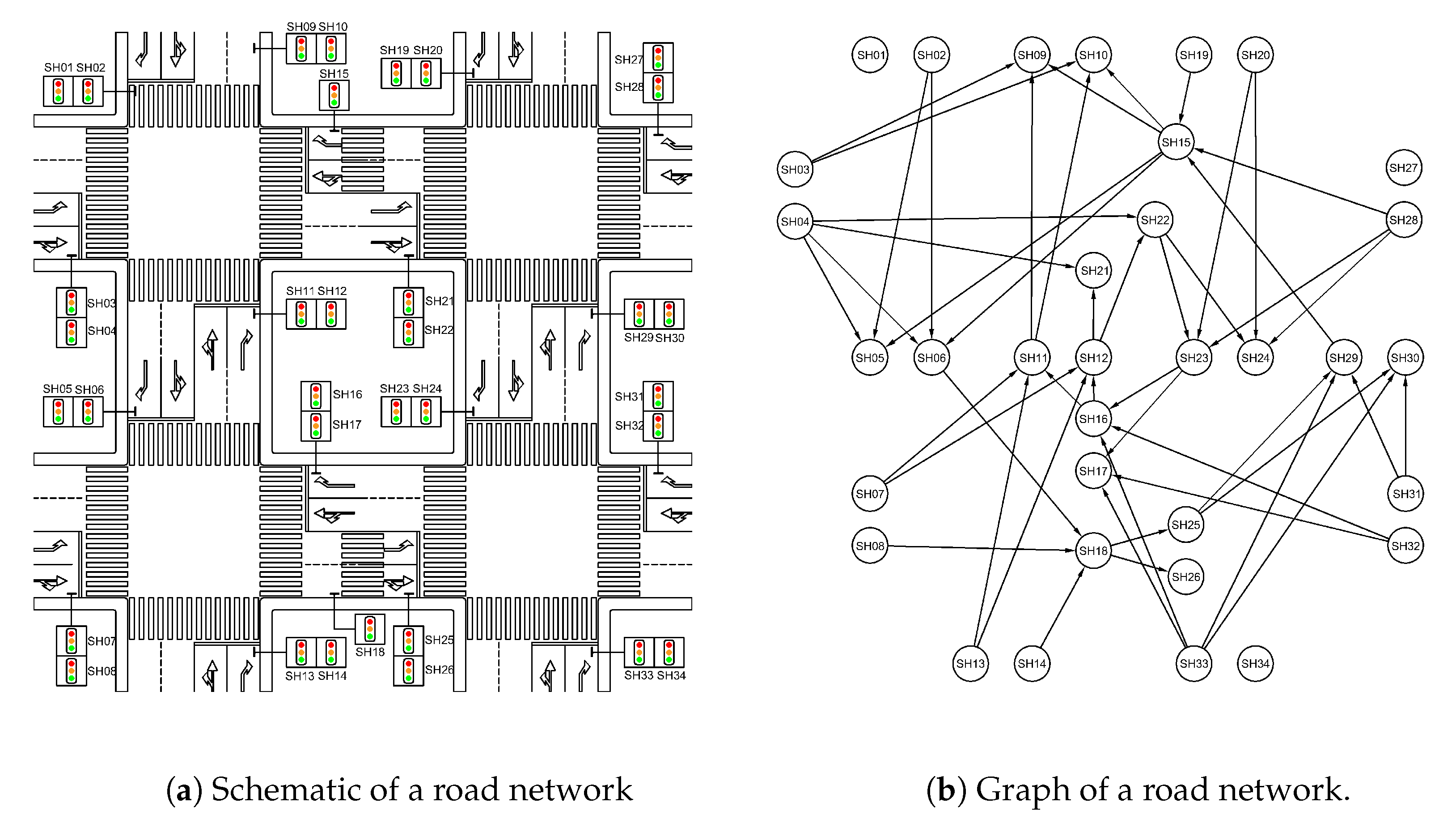
Figure 1 illustrates an example of a road network schema and its corresponding graph representation.

4.1.3. Adjacency Matrix and List

We generate an adjacency matrix A with dimensions $n\times n$, where n is the total number of traffic signals. The elements of the matrix are defined as folows:

$$a_{ij}=\left\{\begin{array}{cc}1\hfill & \mathrm{if}i\to j,\hfill \\ 0\hfill & \mathrm{otherwise}.\hfill \end{array}\right.$$

The adjacency matrix corresponding to the graph in Figure 1 is shown in Equation (1).

$$A=\left[\begin{array}{cccccccccccccccccccc}0& 0& 0& 0& 0& 0& 0& 0& 0& 0& 0& 0& 0& 0& 0& 0& 0& 0& 0& \cdots \\ 0& 0& 0& 0& 1& 1& 0& 0& 0& 0& 0& 0& 0& 0& 0& 0& 0& 0& 0& \cdots \\ 0& 0& 0& 0& 0& 0& 0& 0& 1& 1& 0& 0& 0& 0& 0& 0& 0& 0& 0& \cdots \\ 0& 0& 0& 0& 1& 1& 0& 0& 0& 0& 0& 0& 0& 0& 0& 0& 0& 0& 0& \cdots \\ 0& 0& 0& 0& 0& 0& 0& 0& 0& 0& 0& 0& 0& 0& 0& 0& 0& 0& 0& \cdots \\ 0& 0& 0& 0& 0& 0& 0& 0& 0& 0& 0& 0& 0& 0& 0& 0& 0& 1& 0& \cdots \\ 0& 0& 0& 0& 0& 0& 0& 0& 0& 0& 1& 1& 0& 0& 0& 0& 0& 0& 0& \cdots \\ ⋮& ⋮& ⋮& ⋮& ⋮& ⋮& ⋮& ⋮& ⋮& ⋮& ⋮& ⋮& ⋮& ⋮& ⋮& ⋮& ⋮& ⋮& ⋮& \cdots \end{array}\right]$$

(1)

This matrix represents the connections between traffic signals, where 1 indicates a direct connection from the row signal to the column signal and 0 indicates no direct connection.

Note that the matrix shown in Equation (1) is a truncated version of the full adjacency matrix. For practical reasons, we display only a portion of the matrix, as the complete version would be too large to present in its entirety. This abbreviated form is sufficient to illustrate the structure and content of the adjacency matrix.

From this matrix, we derive an adjacency list representation, which provides a more computationally efficient structure for large networks. The adjacency list consists of a collection of unordered lists, one for each vertex in the graph. For each vertex, its list contains all the vertices to which it has a direct edge. The adjacency list corresponding to the example network is presented below.

• 1: [0]
• 2: [5, 6]
• 3: [9, 10]
• 4: [5, 6, 21, 22]
• ...

In MATLAB, this adjacency list is expressed as a cell array:

• B = {[0], [5, 6], [9, 10], [5, 6, 21, 22], [0], [18], [11, 12], [18], [0], 
•    [0], [9, 10], [21, 22], [11, 12], [18], [5, 6, 9, 10], [11, 12], [0], 
•    [25, 26], [15], [23, 24], [0], [23, 24], [16, 17], [0], [29, 30], [0], 
•    [0], [15, 23, 24], [15],[0], [29, 30], [0], [16, 17, 29, 30], [0]}.

This adjacency list representation provides a concise and efficient way to store and access the network structure, facilitating the use of various traffic optimization algorithms.

4.2. Data Structure

The proposed algorithm and MATLAB function are applicable to any road network and signal head system, regardless of the data source; however, the function requires the data to be structured in a specific format in order to operate correctly.

The necessary data for executing Adjacency_list_of_signal_heads are as follows:

• Reference numbers of the network links, NoOfLinks: These must be integer values stored in a row vector of dimension $1\times N_{Link}$, where $N_{Link}$ is the total number of links. Each link corresponds to a position in the vector and a reference number.
• Reference numbers of the signal heads in the network, NoOfSignalHeads: These must be integer values stored in a row vector of dimension $1\times S{H}_N$, where $S{H}_N$ is the total number of signal heads. Each signal head corresponds to a position in the vector and a reference number.
• Reference numbers of the links regulated by signal heads, LinkOfSignalHeads: These must be integer values arranged in a row vector. The index of the vector indicates the signal head that regulates the corresponding link, which is provided by its position in NoOfSignalHeads. There can be multiple signal heads on a link.
• Position of the signal heads relative to the start of the link they regulate, PosOfSignalHeads: These must be double values. The start of a link is measured with respect to the direction of traffic flow on that link. The index of this vector indicates the signal head that regulates the corresponding link, and corresponds to the same signal head indicated by its position in NoOfSignalHeads.
• Adjacency list of links, AdjacencyListOfLinks: This variable indicates the relationships between links. It should be expressed as a cell array, where the index represents the position of a link in NoOfLinks and the cell contains a vector with the list of adjacent links provided by their reference numbers. Section 5 (Complementary Results) provides a MATLAB function that generates this variable in a PTV Vissim network.

These data are accessible from most specialized sources of traffic information.

4.3. Algorithm Structure

The objective is to obtain AdjacencyListOfSignalHeads, which is an adjacency list of signal heads with the same structure as AdjacencyListOfLinks. This implies a cell array in which the index represents the position of a signal head in NoOfSignalHeads and the cell contains a vector with the list of adjacent signal heads provided by their reference numbers. This objective is divided into four blocks. Additionally, a main function with three subfunctions has been developed for the first three blocks. The last block is implemented directly within the main function, as follows:

• Finding the signalized links adjacent to a given link, 
  Adjacency_list_of_signal_headed_links: This block finds the signalized links adjacent to each signalized link.
• Finding the first and last signal heads of each signalized link,  
  Signal_heads_at_ends_of_links: This block generates a variable with the signal heads at the beginning and end of each signalized link. The beginning of a link is considered the starting point of the link in the direction of traffic flow.
• Sequencing and assigning signal heads within the same link,  
  Adjacency_list_of_signal_heads_in_link: This block selects and orders the signal heads at different positions of each signalized link. The position of a signal head within a link is referenced from the starting point of the link in the direction of traffic flow.
• Assigning the signal heads to the final adjacency list: This block assigns the last signal heads of a signalized link to the first signal heads of its adjacent signalized links. For each final signal head of a link, the first signal heads of all adjacent signalized links are assigned. The result of this block complements the outcome of the previous block.

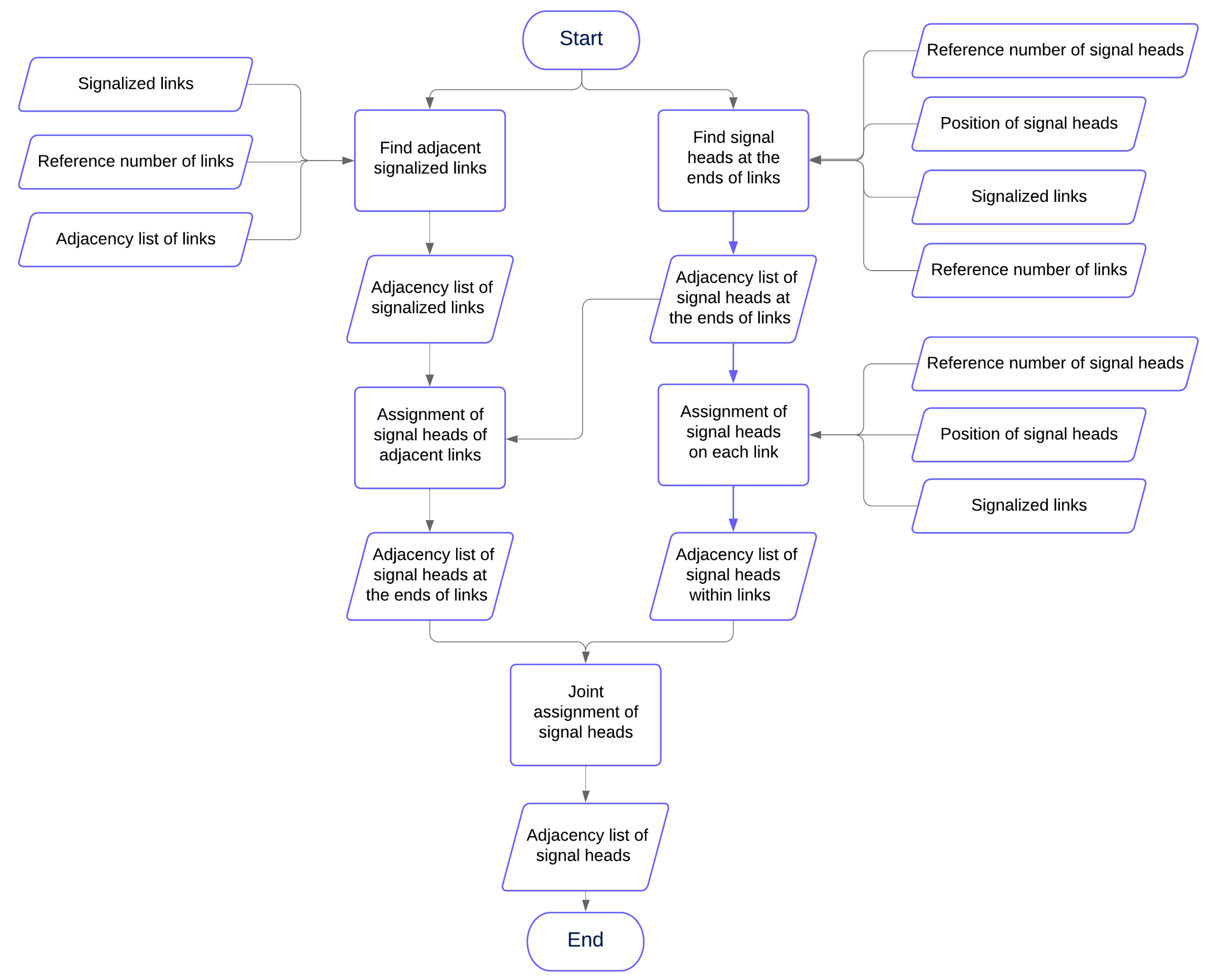
The flowchart of the algorithm is shown in Figure 2.

The results from Blocks 1 and 2 serve as inputs for Blocks 3 and 4. The general algorithm is presented in pseudocode format in Algorithm 1.

Algorithm 1 Main algorithm structure for obtaining an adjacency list of Signal Heads

1: functionAdjacency_list_of_signal_heads(in_link_of_signal_heads, in_adjacency_list_of_links, in_no_of_links,      in_pos_of_signal_heads, in_no_of_signal_heads) 2:     // Generate adjacency list of signalized links 3:     adjacency_list_of_signal_headed_links =         Adjacency_list_of_signal_headed_links(in_link_of_signal_heads,     in_adjacency_list_of_links, in_no_of_links) 4:     // Select signalized links with adjacent signalized links 5:     signal_headed_links =         find_non_empty_indices(adjacency_list_of_signal_headed_links) 6:     // Get signal heads at the beginning and end of signalized links 7:     signal_heads_at_beginning_of_links, signal_heads_at_end_of_links =         Signal_heads_at_ends_of_links(in_link_of_signal_heads, in_no_of_links,      in_pos_of_signal_heads, in_no_of_signal_heads) 8:     // Find links with multiple signal heads (in different positions) 9:     links_with_several_signal_heads =         find_links_with_multiple_signal_heads(signal_heads_at_beginning_of_links,       signal_heads_at_end_of_links) 10:     // Get the sequence of signal heads within each signalized link 11:     out_adjacency_list_of_signal_heads =         Adjacency_list_of_signal_heads_in_link(links_with_several_signal_heads,      in_pos_of_signal_heads, in_no_of_signal_heads, in_link_of_signal_heads) 12:     // Assign adjacent signal heads to the output list 13:     for each link in signal_headed_links do 14:             signal_heads_at_end_of_link =              find_final_signal_head_indices(signal_heads_at_end_of_links, link) 15:             adjacent_links_of_link =              find_adjacent_link_indices(adjacency_list_of_signal_headed_links, link) 16:             signal_heads_at_beginning_of_adjacent_links = [] 17:             for each adjacent_link in adjacent_links_of_link do 18:                add_initial_signal_heads(signal_heads_at_beginning_of_adjacent_links,     signal_heads_at_beginning_of_links, adjacent_link) 19:         end for 20:         for each final_signal_head in signal_heads_at_end_of_link do 21:                assign_adjacent_signal_heads(out_adjacency_list_of_signal_heads,     final_signal_head, signal_heads_at_beginning_of_adjacent_links) 22:         end for 23:   end for 24: end function

4.3.1. Block 1: Identifying Adjacent Signalized Links

Block 1 is the most complex, and requires a detailed description. It consists of two functions. The first, adjacency_list_of_signal_headed_links, generates a cell array representing the signalized adjacent links of the entire road network. Each cell index represents the index of a signalized link in NoOfLinks. The cells are vectors that indicate the list of adjacent signalized links originating from the link provided by its index. The second function, adjacent_signal_headed_links, is used internally by the first to identify the adjacent signalized links for each link.

The function adjacency_list_of_signal_headed_links takes three arguments:

• A row vector of signalized links (in_link_of_signal_heads).
• A cell array of adjacency lists of all links (in_adjacency_list_of_links).
• A row vector of reference numbers for all links (in_no_of_links).

Initially, it identifies the unique signalized links to avoid duplication. Then, for each unique signalized link, it finds the adjacent signalized links using the

• adjacent_signal_headed_links function and stores them in an output cell array.

The adjacent_signal_headed_links function recursively searches for adjacent signalized links. It begins with an initial link, for which it explores all adjacent links. A temporary list (temp_visited_links) is used to keep track of visited links and avoid infinite loops. For each adjacent link, it checks if whether or not it is a signalized link; if it is, then the link is added to the output list. If the adjacent link has not been visited and is not a signalized link, then the function calls itself recursively to explore the adjacent links of the current link. Algorithm 2 shows the pseudocode for Block 1.

This approach allows for constructing a representation of the road network that identifies how signalized links are connected to each other, which is useful for traffic analysis, simulations, and signal head optimization. Recursion and handling of temporary lists are key to this process, allowing for efficient exploration and avoiding the need to revisit links that have already considered.

Consider the network of links represented in Figure 3a and its corresponding schematic representation in Figure 3b, where the directed lines represent the links and the cross-lines represent the signal heads.

The function adjacency_list_of_signal_headed_links, corresponding to Block 1, takes the following input parameters and provides the output:

Inputs:

• in_link_of_signal_heads = [1, 9, 11]
• in_adjacency_list_of_links = {[2, 8], [3, 11], 0, 0, [4, 9], [5, 12],
• [2, 8], [4, 9], 0, [3, 11], [5, 12], 0}
• in_no_of_links = [1, 2, 3, 4, 5, 6, 7, 8, 9, 10, 11, 12].

Output:

• out_adjacency_list_of_signal_headed_links = {[3, 9], 0, 0, 0, 0, 0, 0, 0, 0, 0, 9}.

Algorithm 2 Pseudocode for obtaining traffic light links adjacent to a given link

1: functionAdjacency_list_of_signal_headed_links(in_link_of_signal_heads, in_adjacency_list_of_links, in_no_of_links) 2:     // Select unique signalized links 3:     unique_link_of_signal_heads =         unique(in_link_of_signal_heads) 4:     // Initialize output list 5:     out_adjacency_list_of_signal_headed_links =         cell(1, length(unique_link_of_signal_heads)) 6:     // Create a map for link correspondence 7:     link_map =         containers.Map(in_no_of_links, 1:length(in_no_of_links)) 8:     // Generate adjacent signalized links for each signalized link 9:     for ii = 1:length(unique_link_of_signal_heads) do 10:             current_link = unique_link_of_signal_heads(ii) 11:             index = link_map(current_link) 12:             out_adjacency_list_of_signal_headed_linksindex =              sub_adjacent_signal_headed_links(current_link, containers.Map(’KeyType’, ’double’, ’ValueType’, ’logical’), in_link_of_signal_heads, in_adjacency_list_of_links, link_map) 13:     end for 14: end function 15: functionsub_adjacent_signal_headed_links(in_initial_link, temp_visited_links, in_link_of_signal_heads, in_adjacency_list_of_links, link_map) 16:     // Initialize output variable 17:     sub_out_adjacent_signal_headed_links = [] 18:     // Add initial link to visited links if not already present 19:     if  isKey(temp_visited_links, in_initial_link) then 20:             temp_visited_links(in_initial_link) = true 21:     end if 22:     // Get adjacent links of the initial link 23:     number_of_initial_link = link_map(in_initial_link) 24:     adjacent_links = in_adjacency_list_of_linksnumber_of_initial_link 25:     if empty(adjacent_links) then 26:             return sub_out_adjacent_signal_headed_links 27:     end if 28:     for i = 1:length(adjacent_links) do 29:             adjacent_link = adjacent_links(i) 30:             if  isKey(temp_visited_links, adjacent_link) then 31:                    temp_visited_links(adjacent_link) = true 32:         else 33:                Continue 34:         end if 35:         if ismember(adjacent_link, in_link_of_signal_heads) then 36:                sub_out_adjacent_signal_headed_links =          [sub_out_adjacent_signal_headed_links, adjacent_link] 37:         else 38:            sub_out_adjacent_signal_headed_links =          [sub_out_adjacent_signal_headed_links, sub_adjacent_signal_headed_links(     adjacent_link, temp_visited_links, in_link_of_signal_heads, in_adjacency_list_of_links, link_map)] 39:         end if 40:   end for 41: end function

4.3.2. Block 2: Identifying the Signal Heads at the Ends of Each Link

This block aims to identify the signal heads located at the beginning and end of each link in a traffic network. This task is performed by the function signal_heads_at_ends_of_links. This function takes four input arguments: in_link_of_signal_heads, which represents the links associated with each signal head; in_no_of_links, a row vector indicating the reference number of the links; in_pos_of_signal_heads, which provides the position of each signal head within its corresponding link; and in_no_of_signal_heads, a row vector indicating the reference number of the signal heads.

First, the function obtains the unique links from the list in_link_of_signal_heads using the unique function. Then, it initializes two output cells, out_signal_heads_at_beginning_of_links and out_signal_heads_at_end_of_links, which store the signal heads at the beginning and end of each link, respectively.

Next, the function iterates over each unique link. Within the loop, it finds the signal heads associated with each link using the find function, then obtains the indices and positions of these signal heads. To determine which signal heads are at the beginning and end of the link, the function uses min and max to find the minimum and maximum positions, respectively.

Finally, the function assigns the signal heads corresponding to the minimum and maximum positions to the output cells out_signal_heads_at_beginning_of_links and

• out_signal_heads_at_end_of_links. Thus, upon completion, the output cells contain the signal heads at the beginning and end of each link in the traffic network.

Algorithm 3 shows the pseudocode for Block 2.

Algorithm 3 Pseudocode for obtaining the signal heads at the ends of the links

1: functionSignal_heads_at_ends_of_links(in_link_of_signal_heads, in_no_of_links, in_pos_of_signal_heads, in_no_of_signal_heads) 2:     // Get the unique links 3:     unique_links = unique(in_link_of_signal_heads) 4:     // Initialize the outputs 5:     out_signal_heads_at_beginning_of_links = cell(1, length(in_no_of_links)) 6:     out_signal_heads_at_end_of_links = cell(1, length(in_no_of_links)) 7:     // For each unique link, get the positions and indices of the signal heads 8:     for unique_link in unique_links do 9:           // Get the signal heads for each link 10:         signal_heads_of_link = find(in_link_of_signal_heads == unique_link) 11:         // Get the indices of the signal heads of the link 12:         indices_of_signal_heads_of_link = in_no_of_signal_heads(signal_heads_of_link) 13:         // Get their positions 14:         positions_of_signal_heads_of_link =           in_pos_of_signal_heads(signal_heads_of_link) 15:         // Find the minimum and maximum positions of the signal heads of the link 16:         [~, position_of_first_signal_head] = min(positions_of_signal_heads_of_link) 17:         [~, position_of_last_signal_head] = max(positions_of_signal_heads_of_link) 18:         // Assign the signal heads at the beginning and end of the link to the outputs 19:         out_signal_heads_at_beginning_of_linksunique_link =           indices_of_signal_heads_of_link(position_of_first_signal_head) 20:         out_signal_heads_at_end_of_linksunique_link =           indices_of_signal_heads_of_link(position_of_last_signal_head) 21:     end for 22: end function

The signal_heads_at_ends_of_links function parameters for the case shown in Figure 3 are as follows:

•  Inputs:

  -

  in_link_of_signal_heads = [1, 9, 11].

  -

  in_no_of_links = [1, 2, 3, 4, 5, 6, 7, 8, 9, 10, 11, 12].

  -

  in_pos_of_signal_heads = [8, 2, 7].

  -

  in_no_of_signal_heads = [1, 2, 3].

•  Outputs:

  -

  out_signal_heads_at_beginning_of_links = {1, 0, 0, 0, 0, 0, 0, 0, 2, 0, 3}.

  -

  out_signal_heads_at_end_of_links = {1, 0, 0, 0, 0, 0, 0, 0, 2, 0, 3}.

4.3.3. Block 3: Sequencing and Assigning Signal Heads Within the Same Link

This block creates and assigns a sequence of signal heads within each signalized link in a traffic network using a function called adjacency_list_of_signal_heads_in_link. This function takes four input arguments: in_links_with_several_signal_heads, which is a row vector of those links that have more than one traffic light along with in_pos_of_signal_heads, in_no_of_signal_heads, and in_link_of_signal_heads, which have been defined previously.

It can be observed that several subfunctions of the main function require input parameters. These parameters are either declared in the call to the main function, or obtained from it.

The adjacency_list_of_signal_heads_in_link function begins by initializing the output variable out_adjacency_list_of_signal_heads_in_link as a cell array with a length equal to the number of signal heads. This array stores the sequence of traffic lights for each link.

The main process is carried out within a for loop that iterates over each link that has more than one signal head. For each link, the function identifies the signal heads belonging to that link (number_of_signal_heads_in_link) and retrieves their numerical identifiers (no_of_signal_heads_in_link) and positions (pos_of_signal_heads_in_link).

Then, the function calculates the sequence of signal heads within the link using the unique function to identify unique positions of signal heads and the accumarray function to group the signal heads by their unique position, thereby creating a sequence based on the position of the signal heads within the link.

Finally, if a link has signal heads at more than one unique position, the function assigns the sequence of signal heads to the output variable. This is done by iterating over each group of traffic lights in the calculated sequence and assigning to each traffic light the list of numeric identifiers of the signal heads in the next position. This creates an adjacency list that represents the sequence of signal heads within each link.

Algorithm 4 shows the sequence followed in Block 3 in pseudocode form.

Algorithm 4 Pseudocode for finding and assigning the sequence of traffic lights within each signalized link

1: functionAdjacency_list_of_signal_heads_in_link(       in_links_with_several_signal_heads, in_pos_of_signal_heads, in_no_of_signal_heads, in_link_of_signal_heads) 2:     // Initialize the output 3:     out_adjacency_list_of_signal_heads_in_link = cell(1,       length(in_no_of_signal_heads)) 4:     // Iterate over links with more than one signal head 5:     for each link in in_links_with_several_signal_heads do 6:         // Get the signal head numbers in the current link 7:         link_signal_heads =           Find(in_link_of_signal_heads == link) 8:         // Sort the signal heads by position 9:          sorted_indices =           Sort(in_pos_of_signal_heads(link_signal_heads)) 10:        sorted_signal_heads = in_no_of_signal_heads(link_signal_heads(sorted_indices)) 11:        // Assign the sequence of signal heads to the output 12:        for jj = 1 to numel(sorted_signal_heads) - 1 do 13:                out_adjacency_list_of_signal_heads_in_link{sorted_signal_heads(jj)} =     sorted_signal_heads(jj + 1) 14:         end for 15:   end for 16: end function

For the case in Figure 3, there are no multiple signal heads in different positions in any link; therefore, this function does not modify the adjacency list of signal heads.

• Inputs:

  -

  links_with_several_signal_heads = [].

  -

  in_pos_of_signal_heads = [8, 2, 7].

  -

  in_no_of_signal_heads = [1, 2, 3].

  -

  in_link_of_signal_heads = [1, 9, 11].

• Output:

  -

  out_adjacency_list_of_signal_heads_in_link = [].

4.3.4. Block 4: Assigning the Signal Heads to the Final Adjacency List

Finally, in the body of the main function, adjacency_list_of_signal_heads, calls are made to the previous functions, corresponding to Blocks 1 through 3, and the assignment of the last signal heads of a signalized link to the first of its adjacent signalized links, corresponding to Block 4.

For the case in Figure 3, the input and output parameters provided by the adjacency_list_of_signal_heads function is as follows:

• Inputs:

  -

  in_link_of_signal_heads = [1, 9, 11].

  -

  in_adjacency_list_of_links = {[2, 8], [3, 11], 0, 0, [4, 9], [5, 12], [2, 8], [4, 9], 0, [3, 11], [5, 12], 0}.

  -

  in_no_of_links = [1, 2, 3, 4, 5, 6, 7, 8, 9, 10, 11, 12].

  -

  in_pos_of_signal_heads = [8, 2, 7].

  -

  in_no_of_signal_heads = [1, 2, 3].

• Output:

  -

  out_adjacency_list_of_signal_heads = {[2, 3], 0, 2}.

4.4. Experiments

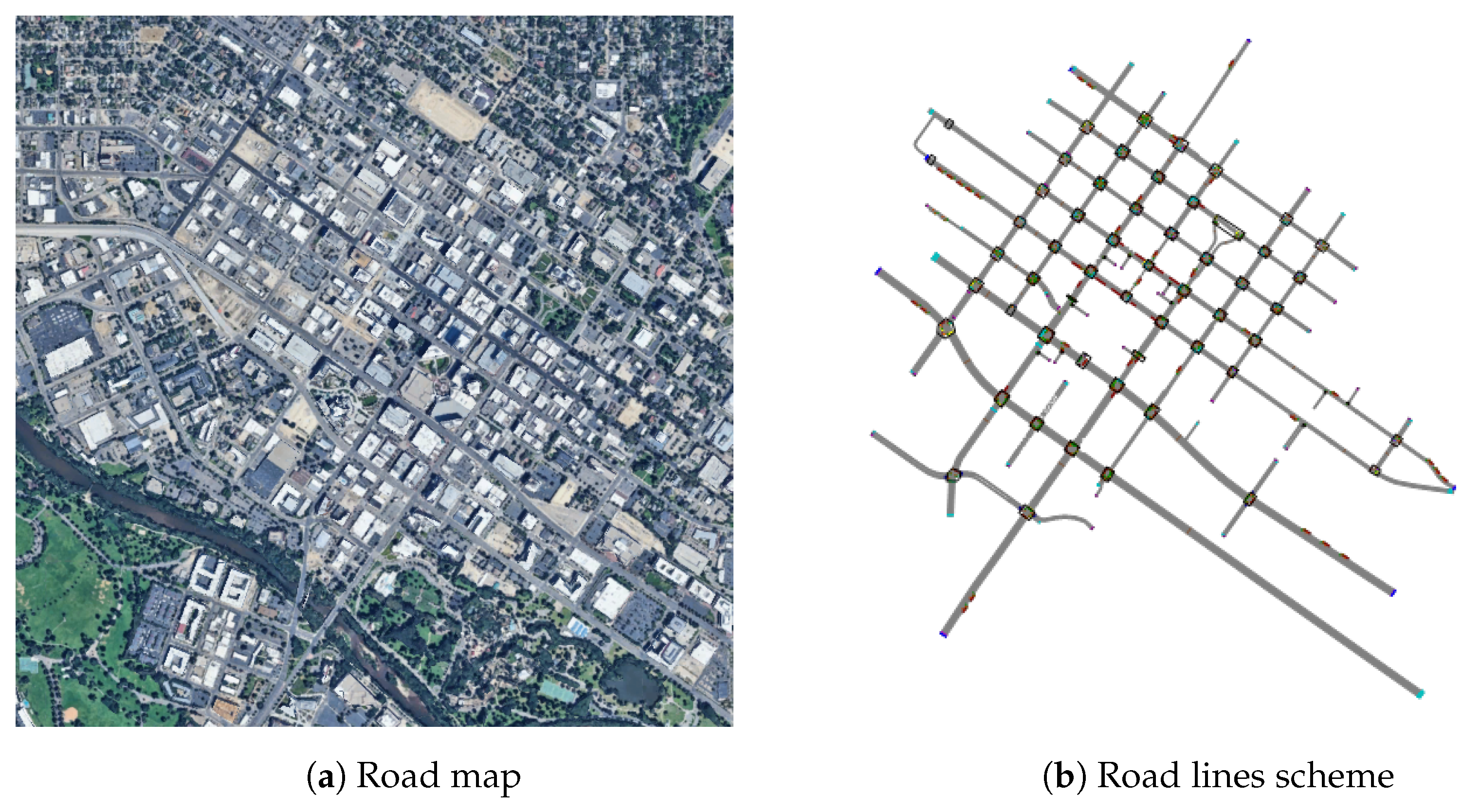
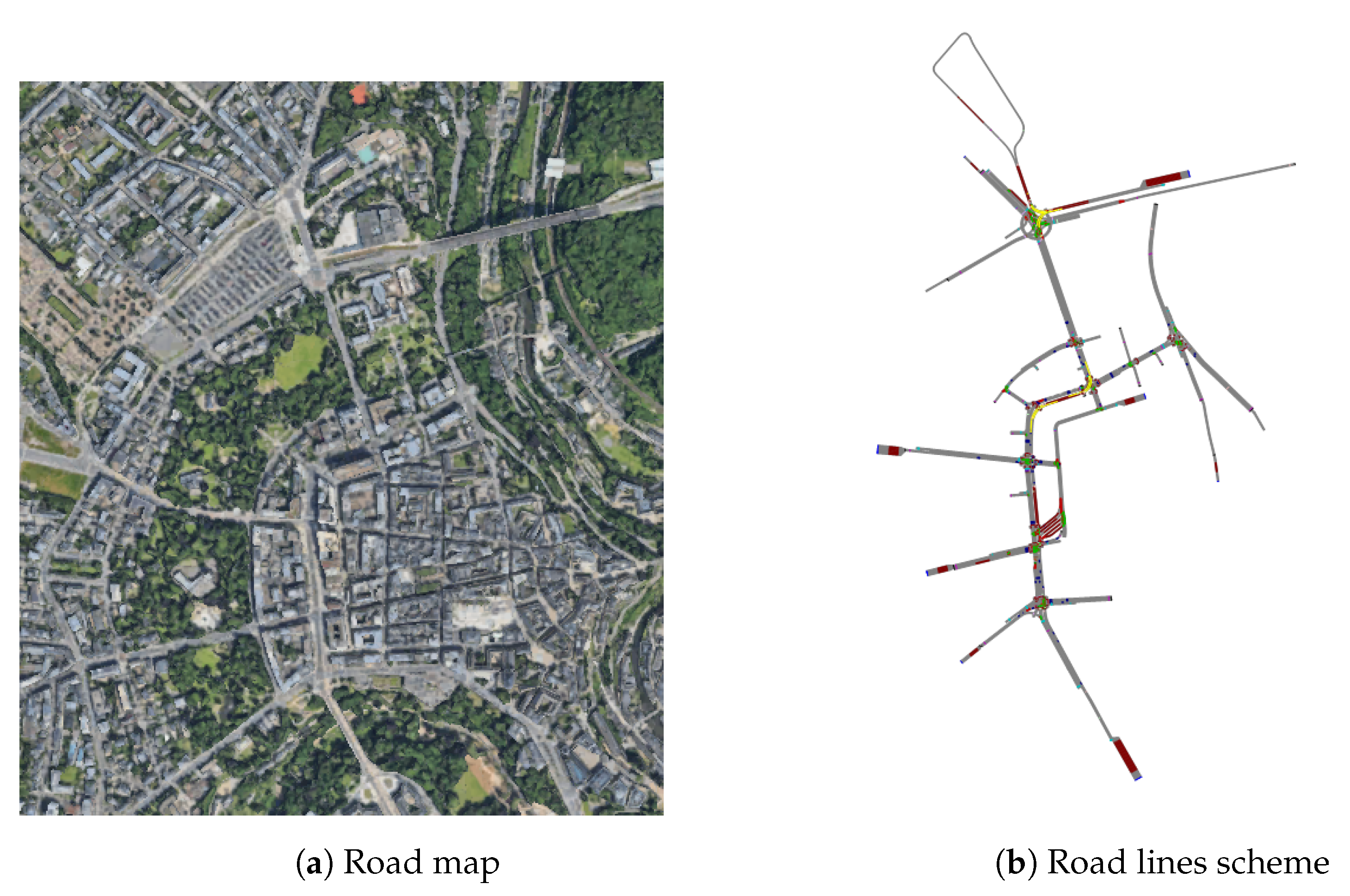
To verify the effectiveness of the proposed algorithm, the developed function was executed in MATLAB on three road networks. These networks correspond to regions in London (GB), Boise (US), and Luxembourg (LU), respectively.

The experiments were conducted using MATLAB R2024a. The personal computer we used was equipped with an Intel(R) Core(TM) i5-4310U CPU @2.00GHz 2.60 GHz and 8 GB of RAM running Windows 10 Enterprise 64-bit version 22h2.

As previously mentioned, the adjacency_list_of_signal_heads function has the following input and output parameters:

• Inputs:

  -

  in_link_of_signal_heads.

  -

  in_adjacency_list_of_links.

  -

  in_no_of_links.

  -

  in_pos_of_signal_heads.

  -

  in_no_of_signal_heads.

• Output:

  -

  out_adjacency_list_of_signal_heads.

The networks selected for the experiments exhibited different network topologies. Figure 4, Figure 5 and Figure 6 display the maps (left) and road networks (right) used in the experiments.

The complete implementation of the proposed algorithm is provided in the Supplementary Materials accompanying this paper. The source code is written as a MATLAB function, and includes the full algorithm for generating adjacency lists. Additionally, we have included the datasets used for our experiments, specifically London_dataset.mat, Boise_dataset.mat, and Luxembourg_dataset.mat. These datasets enable the reproduction of the experiments presented in this study, allowing researchers to validate and build upon our findings.

5. Complementary Codes

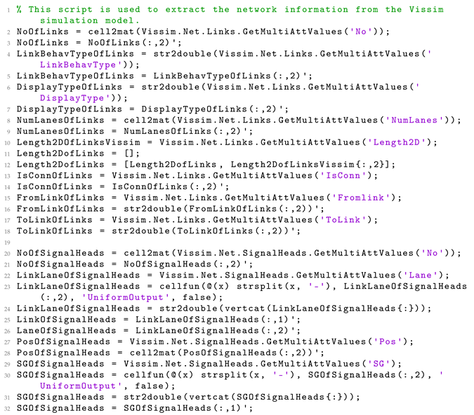
The input parameters of the proposed algorithm can be obtained from various data sources. Users of PTV Vissim can import data from multiple example networks or from OpenStreetMap (OSM). The PTV COM Interface allows for extracting network information and issuing commands from programming environments such as MATLAB, VBA, VBS, Python, C#, C++, and Java. However, the data format does not directly match the structure of the functions presented in this paper. The Listing 1 shows a MATLAB script for importing some data on links and signal heads from a PTV Vissim network and formatting them according to the proposed functions.

Listing 1. MATLAB script for obtaining link and signal head data from a PTV Vissim network.

Most of the input parameters required to run the proposed algorithm can be directly obtained from the data source. However, it is necessary to manipulate the link data to generate the adjacency list of links. Listing 2 presents a MATLAB function adjacency_list_of_links for PTV Vissim users, which generates the adjacency list of links. To call this function according to the parameters mentioned above, it is recommended to enter the following command in the command window:

• [AdjacencyListOfLinks] =
• Adjacency_list_of_links(NoOfLinks, FromLinkOfLinks, ToLinkOfLinks);

Listing 2. MATLAB function code for obtaining the adjacency list of links in an urban network.

6. Results

Ten experiments were conducted for each network to estimate the average execution time.

Table 1. Road element data and average execution time of the networks.

Network	Number of Links	Number of Signalized Intersections	Number of Signal Heads	Execution Time (s)
London (GB)	8372	240	265	63.564
Boise (US)	720	72	547	0.48
Luxembourg (LU)	416	25	126	0.23

lists the numbers of links and signal heads for each network along with the average execution times of the adjacency_list_of_signal_heads function.

7. Discussion

The algorithm for generating adjacency lists presented in this paper offers a novel perspective on traffic light management by focusing on the structural relationships within the network. While this method does not directly control traffic light timing, it provides a crucial foundation for understanding network topology, which is essential for effective traffic light coordination.

7.1. Complementing Existing Systems

While the adjacency list focuses on establishing the structural relationships between traffic lights, it is important to note that this method is designed to complement existing traffic light timing management systems, not replace them. It serves as a valuable tool that can be integrated with dynamic timing algorithms to enhance their performance. By providing a clear map of how traffic lights are interconnected, our method allows timing optimization algorithms to make more informed decisions while taking into account the potential ripple effects of timing changes across the network. For instance, when adjusting the timing of a specific traffic light, adjacency information can quickly identify which other lights in the network might be affected, allowing for more holistic and efficient timing adjustments. This synergy between structural representation and dynamic timing management can lead to more sophisticated and responsive traffic control systems, addressing both the spatial relationships between traffic lights and their temporal coordination.

The adjacency list of a complete network has the potential to significantly enhance advanced traffic optimization techniques such as Spatio-Temporal Multi-Agent Reinforcement Learning (STMARL). The integration of our method with STMARL could lead to more efficient and effective traffic light control systems. To understand how this integration could be beneficial, it is important to first examine the key stages of STMARL:

• Construction of the directional traffic light adjacency graph: STMARL begins by building a graph based on the spatial structure of traffic lights. In this graph, each traffic light is represented as a node and direct connections between lights are represented as edges. This graph captures the spatial relationships and potential interactions between traffic lights in the network.
• Integration of temporal information: Historical traffic records are incorporated with current traffic status using a Recurrent Neural Network (RNN) structure. This stage allows the model to capture temporal dependencies in traffic patterns, enabling it to make decisions based not just on current conditions but also on how traffic has behaved over time.
• Modeling of spatial relationships: A Graph Neural Network (GNN) with an attention mechanism is used to model relationships and cooperation between multiple traffic lights. This stage allows the model to understand how changes at one traffic light might affect others in the network, facilitating coordinated decision-making.
• Distributed decision-making: Each traffic light makes decisions independently using deep Q-learning. This approach allows for scalability in large networks, as each light can make decisions based on local information and the processed information from the GNN.
• Iterative relational reasoning: The GNN allows for efficient and iterative relational reasoning between traffic lights through message passing on the graph. This stage enables traffic lights to ‘communicate’ and adjust their decisions based on the states and actions of other lights in the network.
• Joint optimization: STMARL jointly optimizes the control of multiple traffic lights, considering their spatiotemporal interdependencies. This holistic approach aims to improve overall traffic flow across the entire network, rather than just optimizing individual intersections.

These stages work together to create a sophisticated system for traffic light control that considers both the spatial structure of the road network and the temporal patterns of traffic flow. This approach allows for more nuanced and effective traffic management compared to traditional methods that might consider intersections in isolation or rely solely on fixed timing patterns.

The adjacency list is particularly well suited to enhancing the first stage of STMARL. By providing a more efficient and accurate representation of the traffic network structure, our method can significantly improve this initial step.

In STMARL, the adjacency graph $G=(V,E)$ is constructed based on the spatial structure among traffic lights, where V represents the set of nodes (traffic lights) and E represents the set of edges (direct connections between traffic lights). The adjacency list generated by our algorithm aligns perfectly with this representation:

• Direct mapping: Each traffic light in our generated adjacency list corresponds directly to a node in STMARL’s graph. This one-to-one mapping ensures that all traffic lights are accurately represented in the model.
• Edge representation: The connections between traffic lights in the adjacency list can be directly translated into edges in STMARL’s graph. This ensures that the spatial relationships between traffic lights are accurately captured.
• Directionality: Our approach inherently captures the directionality of connections between traffic lights, which is crucial for STMARL’s directional graph. This ensures that traffic flow directions are accurately represented in the model.
• Efficiency: By providing a precomputed adjacency structure, our method can potentially reduce the computational overhead in STMARL’s graph construction phase. This could lead to faster initialization of the STMARL model, especially for large-scale traffic networks.
• Scalability: Our algorithm can easily handle large numbers of traffic lights, which aligns well with STMARL’s goal of managing complex multi-intersection traffic systems.

It is worth noting that while STMARL provides a framework for using a directional traffic light adjacency graph, it does not specify a method for obtaining these relationships in complex real-world traffic networks. Our algorithm approach addresses this gap by providing a systematic method for determining and representing these relationships in larger and more complex urban traffic networks.

Additionally, the adjacency list generated by our algorithm has potential applications in Emergency Vehicle Preemption (EVP) systems. Adjacency lists and matrices enable rapid identification of relevant traffic signals along the route of a priority vehicle, which could significantly enhance response capabilities and efficiency in urban traffic management for emergency vehicles.

7.2. Enhancing Decision-Making in Advanced Traffic Control Systems

Our algorithm for generating adjacency lists significantly enhances the decision-making process in advanced traffic control systems, particularly those that rely on graph-based representations of traffic networks. While many modern approaches provide frameworks for using network graphs, they often do not specify how to obtain these relationships in complex real-world traffic networks. Our algorithm addresses this crucial gap.

By providing a comprehensive and accurate representation of the network’s topology, our algorithm allows these systems to make more informed and strategic decisions when modeling the spatial relationships between traffic lights. This is particularly important in approaches that use graph-based models, where the quality of the initial graph structure directly impacts the effectiveness of spatial relationship modeling.

7.3. Scalability and Adaptability

One of the key strengths of our algorithm is its scalability, which directly addresses a common limitation in many current traffic management systems. While many approaches demonstrate their effectiveness on small networks (for instance, STMARL uses a network of four traffic lights), our algorithm has been tested on networks with 547 traffic light, demonstrating its ability to handle more realistic urban scenarios.

As urban areas continue to grow and traffic networks become increasingly complex, our algorithm can easily update the adjacency list to reflect changes in the network structure. This adaptability ensures that the method remains relevant and effective even as cities evolve. For instance, our algorithm can quickly regenerate the adjacency list if new roads are constructed or existing ones are modified, allowing traffic management systems to adapt their models without requiring a complete overhaul.

Furthermore, our algorithm’s efficiency in handling large numbers of traffic lights aligns well with the goals of managing complex multi-intersection traffic systems. This scalability is crucial for the practical implementation of advanced traffic management techniques in real-world scenarios, where hundreds or even thousands of intersections may need to be considered simultaneously.

7.4. Reduction of Computational Cost

Our algorithm for generating adjacency lists can significantly reduce the computational cost in advanced traffic management systems. By providing a precomputed adjacency structure, our method minimizes the overhead associated with the initial graph construction phase, which is especially beneficial for large-scale traffic networks.

Additionally, our algorithm helps to define a more constrained action space in multi-agent systems, reducing the complexity of decision-making processes. The clear structure of the adjacency list also facilitates the division of large networks into manageable subgraphs, enabling efficient distributed processing.

Overall, while empirical studies are needed to quantify the exact reduction in computational cost, our approach suggests potential for enhancing the efficiency of advanced traffic management techniques in real-world applications.

7.5. Limitations and Future Work

While our algorithm offers significant advantages, it is important to acknowledge its limitations. First, the quality, accuracy, and currency of the input data about the road network directly impact the effectiveness of our algorithm. The resulting adjacency list is only as good as the data it is based on. Therefore, ensuring up-to-date and accurate road network information is crucial for the algorithm’s optimal performance. Second, while we believe that our approach has the potential to enhance various advanced traffic management techniques, we currently lack comparative data to quantify these improvements. Future work should focus on empirical studies that measure the actual reduction in computational time or cost when our algorithm is integrated into these advanced techniques. This would provide concrete evidence of the algorithm’s benefits in real-world applications.

Future research could also explore the potential of using our algorithm to divide large urban networks into subgraphs for more manageable processing, potentially addressing computational challenges in very large networks. This could lead to a hierarchical approach to traffic management in which local optimizations are balanced with global network performance. Lastly, as traffic management systems increasingly incorporate real-time data from IoT devices and connected vehicles, future work could investigate how our algorithm-generated adjacency lists could be efficiently updated or augmented with these dynamic data, potentially leading to more responsive and adaptive traffic control systems.

In future work, we intend to apply adjacency lists to Emergency Vehicle Preemption (EVP) systems, allowing for a new perspective. This approach will focus on enhancing the efficiency of traffic signal management for priority vehicles, aiming to improve response times and overall traffic flow in urban environments. By leveraging the structural insights provided by our adjacency lists, we hope to develop adaptive strategies that can dynamically prioritize traffic signals based on real-time conditions and the presence of emergency vehicles.

8. Conclusions

In this paper, we have presented a novel algorithm for generating adjacency lists for traffic light networks. Our method provides a fundamental structural representation of traffic networks, offering several key advantages:

• Efficient network representation: Our algorithm offers a computationally efficient way to generate adjacency lists for complex traffic networks, potentially enabling faster processing and analysis in traffic management systems.
• Scalability: Our method is highly scalable for handling traffic networks of varying sizes, from small intersections to large urban areas.
• Integration potential: Our approach shows promising potential for integration with existing traffic management systems and advanced technologies such as STMARL.
• Foundation for optimization: By providing a clear structural representation of traffic networks, our method lays the groundwork for more sophisticated traffic optimization algorithms.

While our approach focuses on generating static structural relationships within traffic networks, it provides a crucial foundation for understanding network topology. This understanding is essential for effective traffic light coordination, and can potentially enhance the performance of dynamic timing algorithms.

The adjacency lists generated by our algorithm complement existing traffic management systems by offering a comprehensive view of the network’s structure. This allows for more informed decision-making, particularly when considering the ripple effects of changes across the network.

It is important to note that the effectiveness of our algorithm depends on the quality, accuracy, and currency of the input data about the road network. Furthermore, while we believe that our approach has the potential to reduce the computational costs of advanced traffic management techniques, empirical studies are needed in order to quantify these improvements.

In conclusion, our algorithm for generating adjacency lists represents a significant step forward in traffic network representation. By providing an efficient method for capturing the structural relationships within traffic networks, it opens up new possibilities for more sophisticated, responsive, and effective traffic control systems. As urban areas continue to grow and traffic management becomes increasingly complex, methods such as ours will play a crucial role in developing smarter and more efficient transportation networks.