Abstract
Carbon fiber reinforced plastic (CFRP) parts find a rising number of applications as structural components. Therefore, new manufacturing technologies are developed, enabling high volume production of such parts. With those higher volumes, variation management during product design becomes more critical. While manufacturing variations in CFRP materials occur on different scales, detecting and considering those on the meso (ply) scale becomes more important. Thus, the question arises whether such variations can be detected with standardized testing methods. In this study, artificial fiber misalignment has been introduced into the outer plies of standardized tensile specimens to explore the influence of such variations on the mechanical properties. A simulation model was developed to identify these variations and the test results were used to calibrate and optimize the material parameters of the simulation model. The effects of the artificially induced variation were distinguishable in the test data as well as in the simulation models. Furthermore, the simulation models showed good agreement with the experimental data, which leads to the conclusion that the utilized measuring techniques are well suited to characterize the fiber misalignment. The developed simulation models can be used to investigate the effects of fiber misalignment within the product development process without the need for physical testing.
1. Introduction
Composite parts enjoy high popularity in the aerospace and transportation industry due to their lightweighting potential compared to more traditionally used metal components. Significant improvements in design, optimization [1,2] and manufacturing [3] of composite parts have been made over the last years to increase structural and geometrical performance. However, the realization of series production of composite structures remains challenging. Within the raw materials and the manufacturing process steps variations can occur, that inevitably lead to a loss in quality [4]. The quality loss can be observed in various areas, such as geometric quality or structural performance. Geometric quality loss is manifested, for example, in increased warpage or spring-in as well as in dimensional variations [5,6]. Structural performance is reduced through decreased stiffness and strength with respect to mechanical loading behavior [7] and residual stresses [6]. Both are particularly critical for structurally optimized parts, because it leads to a variation from the desired nominal state.
In [8] the wide variety of occurring variations and the corresponding manufacturing process steps are clustered and transformed into a taxonomy of defects. The considered variations occur in the raw material, e.g., resin content, during the manufacturing process, exemplarily pressure and temperature variations of molding process or inconsistent filling leading to voids [9], or in the postprocessing steps, e.g., uncertainties in the datum or the assembly process. A more detailed overview of variation sources along the composite manufacturing processes is given in [10,11]. Variations in fiber orientation, including fiber misalignment and forming induced fiber angle changes, are stated to need further investigations [12], since there are few studies on their effects, like in [13] analyzing the effect of fiber orientation on the spring-in angle. While the variation sources related to composite and process design are stated to be the most important ones regarding geometrical variations [10], they can further influence the parts structural quality.
Variations in composite structures occur at different scales. Variations at the macro scale, e.g., geometric and dimensional variations can be measured well using coordinate measurement machines or optical methods such as 3D scanning, while variations on the meso and micro scale require more effort and specialized equipment. However, effects of variations at the meso and micro scale can be observed on the macro scale, e.g., manufacturing deformations or strength and stiffness variations of the laminate. While variations affect those measures independently of whether woven or unidirectional plies are used, the effect is significantly higher for unidirectional ones due to their high degree of anisotropy. Hereby variations on the meso scale, like ply thickness variations [14], ply and fiber misalignment [15,16] or fiber waviness [17], influencing the stiffness and strength behavior [18], are of high importance.
Variation analysis is a method investigating the influence of variations like fiber misalignment, based on simulation data or experimental data. Simulation-based approaches including variation analysis or optimization suffer from the compromise between the cost of simulation and the simulations output reliability [19]. However, simulation is widely used in variation analysis due to the lower effort compared to investigating variations in physical parts. Especially investigating and measuring big samples to gather statistical data on the variations and their effects comes with very high effort, thus it is rarely performed exhaustively.
Experimental variation analysis, investigating effects on structural performance, mainly focuses on meso scale parameters in a small number of samples, compared to what is realizable with simulation. This can be used to calibrate simulation models, improving their suitability for variation simulation. Calibration is required for a wide variety of simulation models, particularly Finite Element Analysis (FEA), which can be used for a variety of applications such as manufacturing process simulation (e.g., forming, curing, assembly) or structural simulation (e.g., static use case, crash simulation).
Measuring the variations, i.e., fiber misalignment, can be categorized in destructive testing and non-destructive testing. Destructive testing, e.g., using microsections [20], makes it impossible to analyze other properties, possibly impacted by the variations, of the specimens afterwards. Non-destructive testing methods show a wide variety based on different principles, considering eddy current, ultrasonic or micro CT for fiber misalignment [21,22,23]. Besides measuring the variations of the fiber orientation, measuring the effects and inferring the causing variations can be advantageous. The measurement of resulting geometrical variations is very common using tactile or optical measurement systems. Measuring the effects on the structural behavior in standardized tensile testing methods such as ASTM D3039 [24] or DIN ISO 527 [25] is less common.
In the following, the focus is set to variations in fiber orientation, i.e., fiber misalignment, which can originate in different process steps. While misalignments can already be found in the raw material at times, introduced during prepreg manufacturing and rolling [11], variations of the fiber orientation can occur equally during cutting and stacking/placement of the single plies [10,12]. Furthermore, forming, e.g., bending around radii, and draping over double-curved surfaces may lead to additional variations [8]. As already stated, such variations influence the resulting geometry due to changed thermo-mechanical behavior of the laminate as well as permeability, which influences the curing behavior of the laminate. The influence on the structural behavior results from (spatially) changed stiffness and/or changed strength, since the resulting angle between load flux and fiber direction is altered. At the meso scale, effects of the fiber orientation on the structural behavior have been investigated in several studies [26,27,28,29]. For instance, in [26] a study on the effect of fiber orientation in glass fiber reinforced plastics (GFRP) using analytical, numerical and experimental methods is presented. It shows the dependence of the ply and laminate stiffness with respect to the fiber orientation in a range of 0° to 90° to the load direction. The effect of the fiber orientation on the tensile strength was investigated in [28] using three orientations, [0°/90°], [30°/−60°] and [45°/−45°]. A strong decrease in strength in association with a change in failure mode was found. Due to the effects of variations, considering them during product development is essential, requiring tailored methods and tools.
The mentioned studies investigate the effect of fiber orientation on the structural properties of the laminate, but over a wide range of angles. Small variations in fiber orientation, like they emerge from manufacturing, however, have not been analyzed in detail. Investigations regarding the effect of small fiber orientation variations can clarify whether the effects are strong enough to separate them from other variations, seeing predicted deterministic effects from analytical and numerical models in the testing data. Furthermore, the ability of standardized testing methods in measuring the small variations must be verified, in order to perform analyses of fiber misalignment and its effects on the structural behavior. The use of numerical simulation models for material calibration and comparison with the testing results provides useful information on the ability to represent small variations in simulation models and therefore, whether they are suitable for variation simulation. From these issues the following research questions have been derived and will be addressed in this contribution:
- What is the influence and effect of meso scale variations, i.e., fiber misalignment/variation of fiber orientation, on the structural behavior of composite parts?
- To what extent can the variations be determined with standardized tensile testing methods (DIN 527 & ASTM D3039)?
- What accuracy can be achieved by simulation models representing variations on the ply scale?
By answering these questions, we want to gain novel insights in the determination of fiber orientation variations within tensile tests. Furthermore, evaluating the simulation models regarding the representation of small fiber orientation variations shows the suitability of the models for variation simulation. This enables statistical investigations on variations and contributes to increasing the prediction quality of variation simulation and therefore product quality.
To answer these research questions the paper is structured as follows. Section 2 presents the methods used to investigate the correlation of simulation models and experimental tests. In Section 3, first the results of a corresponding experimental test are shown, complemented by the calibration of a material model which is then used for a final evaluative comparison of simulation and experimental data. Section 4 then discusses the findings and their contribution answering the research questions. Additionally, further challenges and developments of variation characterization on the ply level are discussed.
2. Materials and Methods
Determining the influence of variations experimentally and estimate reliable variation distributions of a single parameter is a costly and time consuming. Attempting to compare variations from an experimental setup with the effects of variations in a virtual setup is (computationally) expensive due to the statistical nature of variations [30,31]. To decrease the necessary effort for variation analyses, the authors propose an approach for the evaluation of simulation models, wherein they can represent the effects of variations thoroughly, by introducing such variations artificially. Subsequently, for the statistical variation analysis the evaluated simulation model can be used. In order to introduce artificial variations reliably, the manufacturing process has to be more accurate than the investigated variations. On the one hand, this undermines the need for variation analysis of the investigated variation ranges. On the other hand, it offers the possibility to enhance and evaluate the simulation models, which then can be transferred to other manufacturing processes that are inherently more prone to variations. Additionally, variations from subsequent process steps, such as draping, can be considered, which leads to additional variations that should be investigated in structural simulations. Therefore, the present work uses a highly automated and precise tape laying process to manufacture the needed specimens.
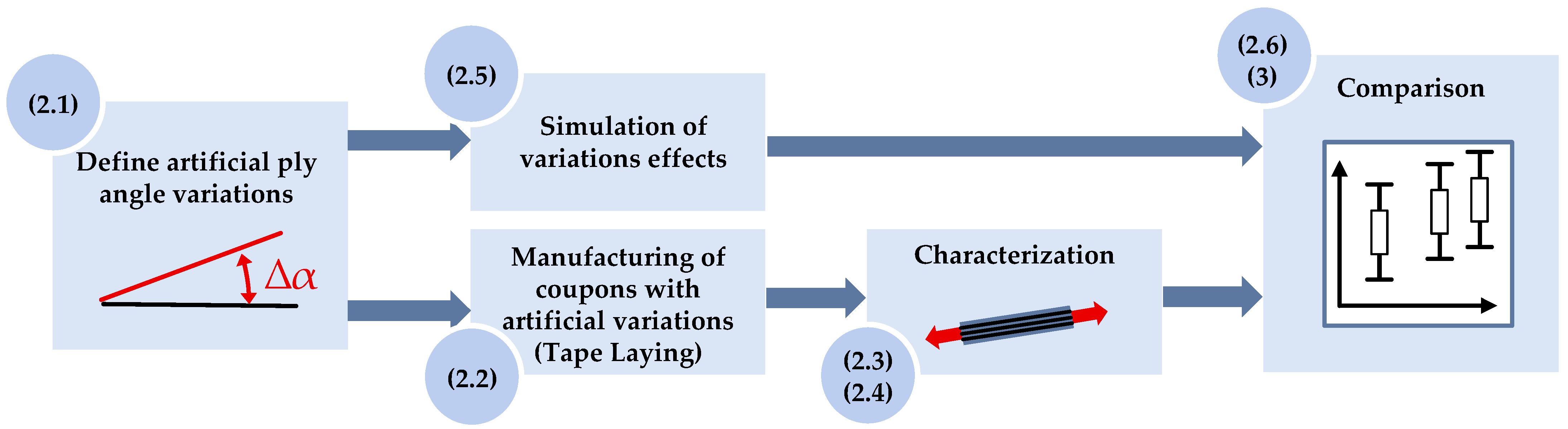
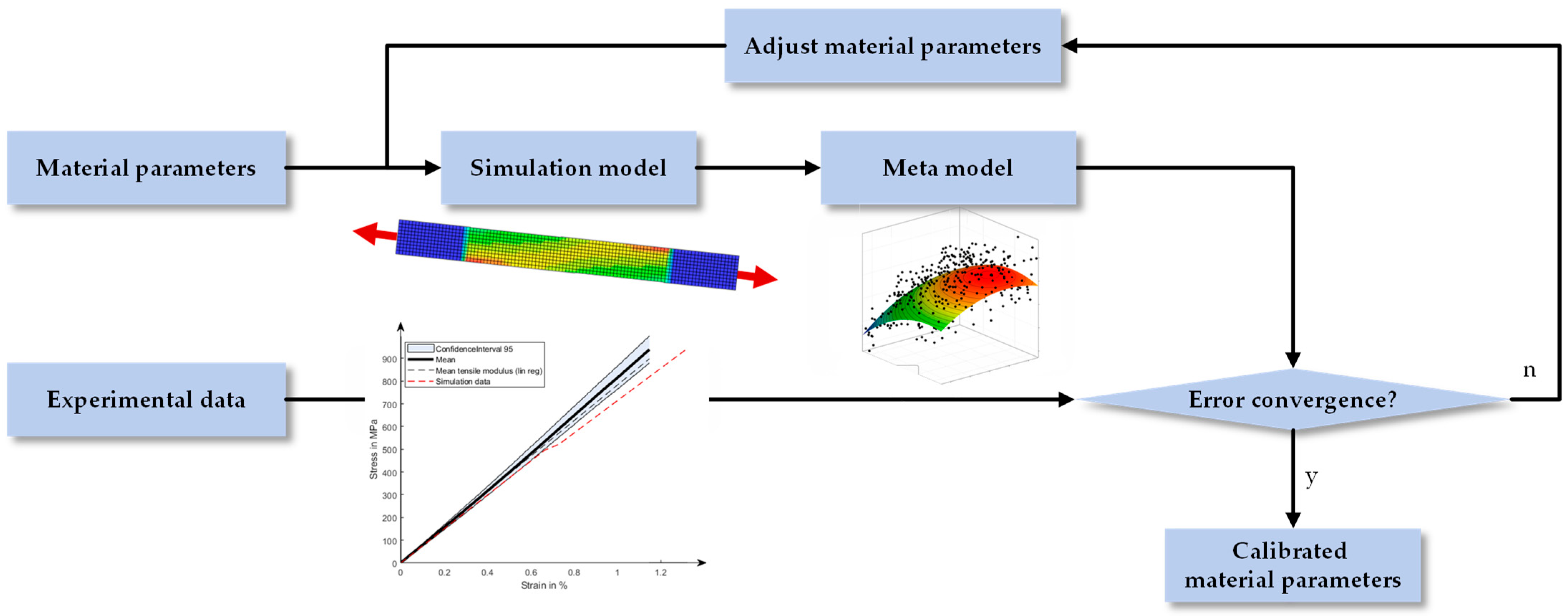
The approach used to evaluate the simulation model is presented in Figure 1. It consists of five steps, starting with the definition of the artificially introduced variations in Section 2.1, as well as the definition of the specimens, lay-up and material. In the presented work we focus on ply angle variations. After the initial definitions two strands are followed. First, the manufacturing of the coupon specimens with the artificial variations are presented in Section 2.2, followed by the experimental setup and characterization in Section 2.3 and Section 2.4. The other strand addresses the modeling and simulation of the variation effects using FEA, presented in Section 2.5. Finally, both, simulation models and experimental test data are merged for model calibration described in Section 2.6 with the results presented in Section 3.
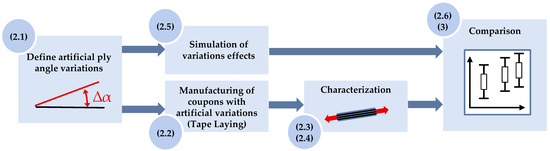
Figure 1.
Approach for the material characterization of composites materials with artificial variations.
2.1. Material and Specimens
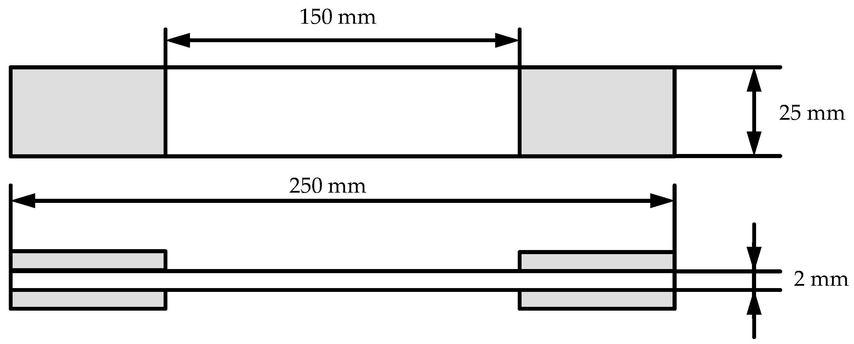
A unidirectional carbon-fiber reinforced epoxy prepreg was supplied by DowAksa, Midland, USA (XForge™ VF P6300) on a 6″ cardboard core with a width of 49.5 mm and no release paper was used. The prepreg DowAksa A42-D012, 24k carbon fibers with a fiber aerial weight of 186 g/m2. The fibers were impregnated with a high-performance epoxy resin system specifically designed for automated processes offering zero tack, fast curing and integrated mold release. The tape material had an average thickness of 0.2 mm. The specimen’s geometry is based on the testing standards ASTM D3039 [24] and ISO 527-4 [32] with minor variations, such as the specimens thickness. The specimen’s geometry is shown in Figure 2. Additional GFRP tabs have been glued to the specimens to improve gripping and reduce the damage from it to avoid premature failure.
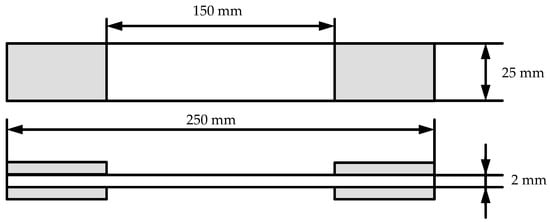
Figure 2.
Specimen geometry with additional tabs for gripping.
The desired specimen thickness of 2 mm is achieved through a 10-ply lay-up. Three different specifications are investigated, testing 5 specimens of each specification. Table 1 provides a detailed overview of the specifications: First a nominal lay-up with 0° ply angles, serving as reference; Second a lay-up with 5° ply angle variation of the top and bottom layers; Third a lay-up with 10° ply angle variation. The two variation specifications are intended on the one hand to avoid coincident errors and on the other hand verify the theoretical loss in stiffness and strength. The variation magnitude is selected in accordance with typical values reported in literature, with standard deviation ranging from approximately 0.5° to 2° [20,33,34], depending on the manufacturing process. This leads to the assumption of a normal distribution of variations and a conformance rate of ±3σ = ±5°. Additionally, local fiber angle variations can be higher for example., due to draping effects. Therefore, the selected variations are considered to be within a reasonable range for evaluating variations in simulation models, with limitations regarding the degree of detail of the modeling.

Table 1.
Investigated laminate lay-ups with artificial variations of the top and bottom layers.
2.2. Manufacturing
Flat composite lay-ups (250 mm × 200 mm) were produced on an automated tape laying machine (Multilayer from FILL, Gurten, Austria) and consolidated in a 20t lab press (LabTech Engineering Co. Ltd., Barnegat, NJ, USA) at 160 °C for 5 min using a 2 mm spacer plate. The process is shown in Figure 3.
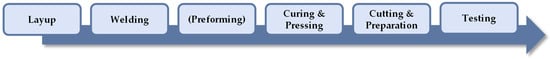
Figure 3.
Manufacturing steps of the Tape Laying Process with the FILL Multilayer.
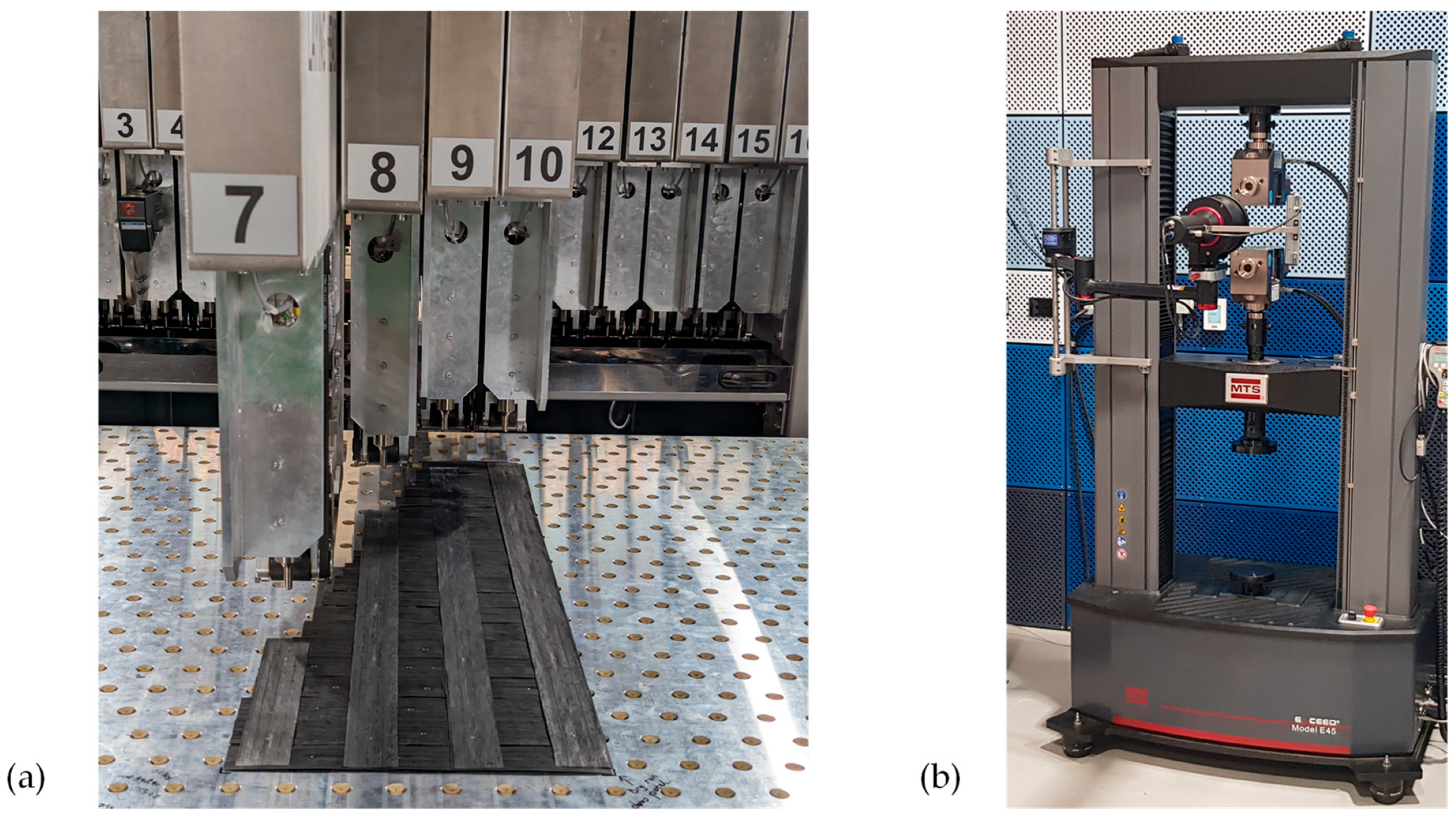
The Multilayer, shown in Figure 4a, utilizes high-precision magnetic linear motors to accurately position the 16 individual laying heads, which can be equipped with bindered dry-fiber, thermoplastic and thermoset tapes to produce flat tailored tape stacks with dimensions up to 1.6 m × 1.6 m. The tapes are deposited onto a vacuum rotary table with 360° of freedom and a position accuracy of 1°. The first layer is held in place by the vacuum table, while each subsequent layer is spot-welded to the previous layers to create a tape stack with sufficient intrinsic rigidity to be picked and placed by either manual or automated processes. The spot-welds, shown in Figure 5, are placed in user-defined locations and the weld parameters need to be adjusted according to the tape material being used.

Figure 4.
Fill Multilayer station (a) with eight laying heads and rotational and translational moveable layup table and universal testing machine (b) performing the tensile tests with an 2D-DIC system.
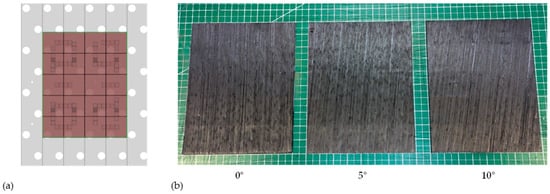
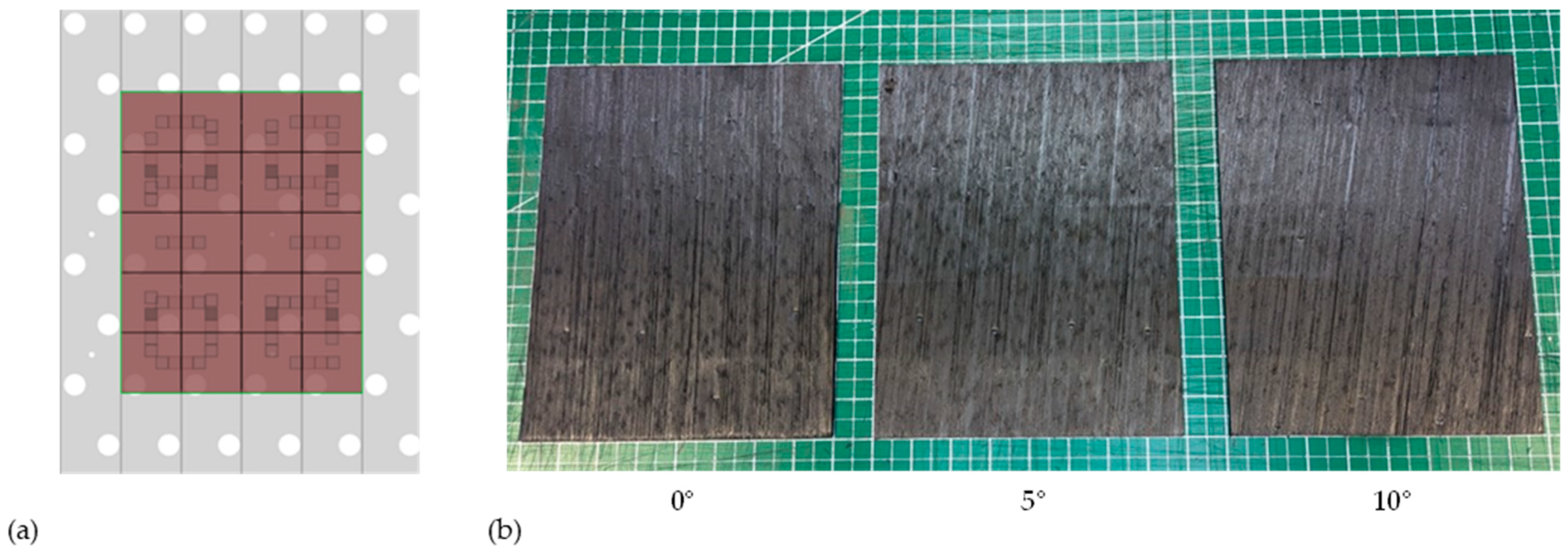
Figure 5.
(a) Lay-up on the vacuum table, with the plate contour (green), the tapes (red with black lines) and welding spots (small squares); (b) Manufactured plates for the three specifications.
The reference lay-up consists of 10 plies (0°/0°/90°/90°/0°)s that were spot welded in strategic locations to create a self-supporting tape-stack. The other plates were produced with 5° and 10° fiber angles (5°/5°/90°/90°/0°)s and (10°/10°/90°/90°/0°)s on the two outermost layers to investigate the influence of fiber angle misalignment on the mechanical properties of the composite.
After adhesive bonding of tabs, the cured composite plates were water-jet cut into tensile test specimens according to ASTM D3039 [24] (250 mm × 25 mm). Thickness and width measurements were taken for all tensile coupons and showed thickness values of 2 mm ± 0.1 mm and width values of 24.9 ± 0.05 mm.
2.3. Experimental Setup
A 100 kN universal testing machine from MTS (Exceed E45 supplied by John Morris Scientific Pty Ltd., Chatswood, NSW, Australia), see Figure 4b, equipped with hydraulic grips and an advantage video-extensometer (AVX) was used to perform tensile tests in accordance with to ASTM D3039. Specimens were placed in the hydraulic grips and tested until failure at a constant crosshead speed of 2 mm/min. The standard 100 kN load cell in combination with the video-extensometer were used to capture the stress-strain curves.
2.4. Laminate Characterization
Laminate properties were calculated in accordance with ASTM D3039 [24], ISO 527-1 [25] and ISO 527-4 [32]. From the recorded stress-strain curves the tensile modulus of the laminate was calculated using linear regression of the stresses in the strain range between 0.05% and 0.25% referred to as regression tensile modulus. The stress calculation represents the engineering stresses of the laminate with reduced physical meaning. More detailed stress analyses would require layer-wise analysis which is not required for the current study.
In addition, a statistical analysis on the experimental data was performed. Mean values and standard deviations were calculated for the tensile modulus and the ultimate tensile strength. Two-sided t-tests were performed in order to determine whether the distributions of the different specifications can be distinguished unambiguously. Furthermore, the stress-strain curves can be evaluated statistically as well. Therefore, the data has been interpolated linearly for the strains until the ultimate failure of the first specimen of a dataset. Subsequently, the interpolated data is used to calculate the mean curve assuming a normal distribution and the 95% confidence interval.
2.5. Modeling
The comparison of variation effects requires the preparation of a simulation model. The simulation model is designed according to the test specimens with the same dimensions and layup. The software package LS-DYNA R11.0 has been used for the numerical modelling and simulation. Fully integrated shell elements are used for discretization, resulting in 1000 elements with an element size of 2.5 mm. The material is modeled using an orthotropic material model with optional brittle failure (*MAT_022 with Chang-Chang failure model [35]) considering laminate shell theory. The simulation model is fixed on one side, while a displacement is applied to the other side, analogous to the experimental boundary conditions. The simulation was performed with an implicit solution algorithm with automatic switching to explicit solving and automatic time stepping. Simulations were terminated if a predefined number (10 for 0°, 100 for 5° and 10°) of elements failed. The material properties used for the initial simulations and the strength parameters can be found in representing the values from the data sheet [36]. The overall structure of the FEA model is given in Figure 6.
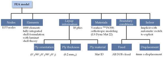
Figure 6.
FEA model structure used for simulation and model calibration.
2.6. Model Calibration
The model calibration procedure attempts to optimize the material parameters of the material model to match the simulation in the best way to the experimental results. The procedure implemented in LS-OPT 7.0 is shown Figure 7. The simulation model described in Section 2.5 provides the basis for calibration, where the material properties have to be defined as parameters. The Young’s modulus of a ply parallel to the fiber direction Ex, Young’s modulus perpendicular to the fiber direction Ey, shear modulus Gxy and the Poisson’s ratio are determined within the calibration, starting with the datasheet values. The adjustment of the material parameters is performed utilizing the genetic optimization algorithm (GA). The GA optimization needs to solve a large number of simulations which results in a high computational effort. To reduce the effort, a metamodel is used for fast evaluation and optimization. During each optimization iteration a space filling sample of 15 points is generated and solved. The results are then used as training data for a kriging model with a Gaussian correlation function. The metamodel is then used to optimize the material parameters in order to minimize the area between the stress-strain curves of the simulation and the experimental results. After convergence or a maximum of 20 iterations the optimization is terminated and the calibrated parameters can be used for further simulations.
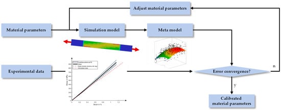
Figure 7.
Model calibration procedure to optimize material parameters to match the simulation results with the experimental results.
The procedure can be further extended by matching multiple load cases or simulations to different curves. Accordingly, a material parameter calibration was performed for the nominal 0° laminate lay-up as well as combined for all three specifications, the 0° lay-up, 5° variations and 10° variations. Consequently, the calibration with all three specifications combined is a Pareto optimization, where improving the curve fit matching of one specification can lead to a worsened other curve fit. Therefore, not only a single optimal solution exists but a so-called Pareto front which describes the points where the described behavior applies.
3. Results
The following section presents the results answering the research questions. First in Section 3.1, the experimental results are evaluated in terms of the effects of variations and mechanical performance. In addition, the potential to study the effects of variation using standardized test methods is investigated. In Section 3.2, the material calibration procedure is applied to obtain the best fitting material parameters, which can then be used for further investigations regarding the evaluation of modeling variations in simulation in Section 3.3.
3.1. Mechanical Properties
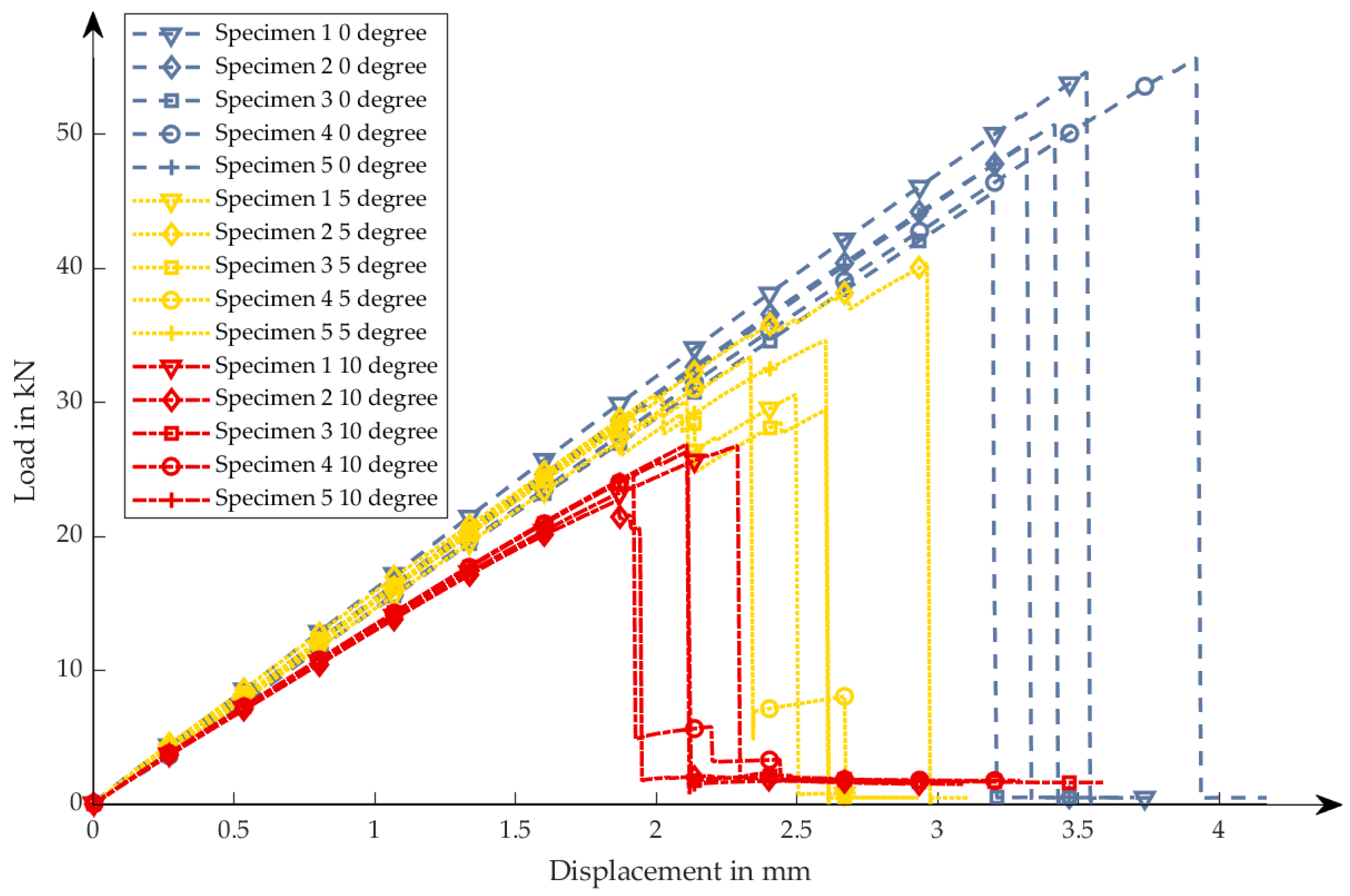
First a brief overview of the performed tests for the three specifications, defined in Section 2.1 and have been tested according to Section 2.3, is given in Figure 8 showing the load displacement curves of all 5 specimens of each specification. Within one specification the variations are reasonable. While for small loads and displacements the variations are small, for higher loads and displacements the variations increase especially for the 0° specimens. Differences in the steepness of the curves can be seen especially for the 10° specification. Analyzing the failure behavior shows clear differences between the three specifications. The 0° nominal specification shows the highest failure loads, followed by the 5° variation specimens and worst of all, the 10° specimens. Furthermore, the values in each specification vary strongly. Between the different specifications the failure behavior shows different effects as well. While the nominal laminate lay-up (0°) shows spontaneous ultimate failure, the 5° variation specification samples have first failures observable by load reduction and afterwards another increase in load. Those effects can be explained with first ply failures which are then compensated by other layers, which leads to another increase in load and thus ultimate failure.
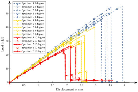
Figure 8.
Load-displacement curves of all tested specimens clustered into the three variation specifications: 0° (blue), 5° (yellow), 10° (red).
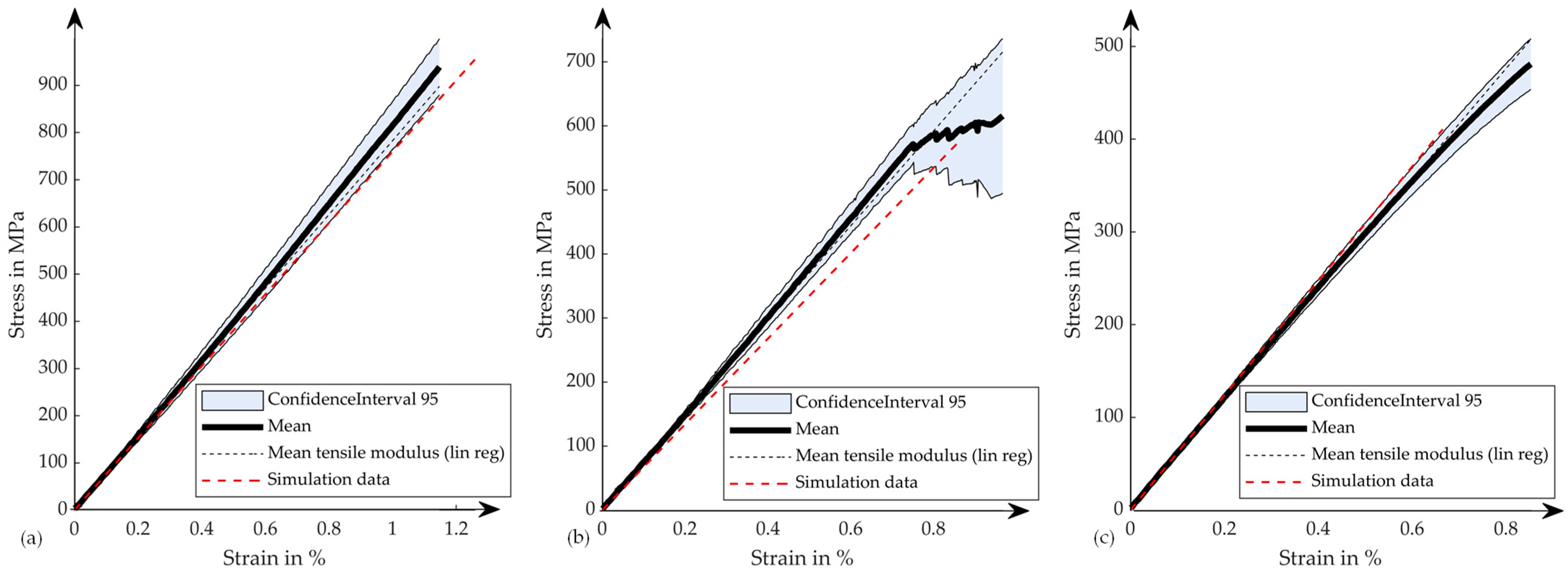
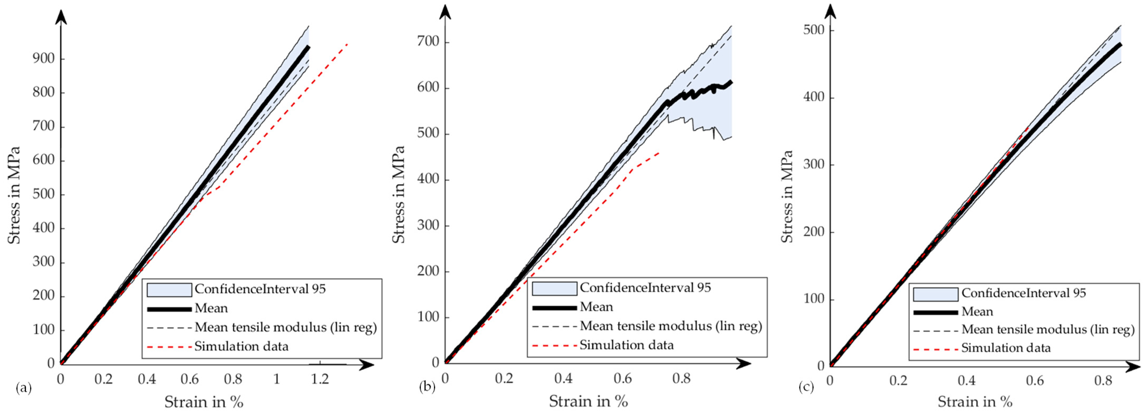
The stress-strain curves are derived from the measured forces and strains for each specimen. For each variation specification the mean curve and 95% confidence interval are calculated assuming normal distribution of the curves. The mean curves are calculated until ultimate failure of the first specimen occurs. The diagrams in Figure 9 show the stress-strain curves of the three variation specifications. The 0° specification shows linear behavior throughout the entire curve until the point of failure. The stress variation, i.e., confidence interval, increases at higher strains, though it remains in an acceptable range. Furthermore, the laminate tensile modulus is calculated from the single stress-strain curves according to Section 2.4. The mean values of the specifications are shown in Figure 9. It shows a slight underestimation of the stiffness at higher strains, yet remains within the confidence interval. Generally, the nominal specification shows the expected linear behavior of the composite material with acceptable variations of the stress-strain curves, which makes it a good reference for comparison to the variational specifications.
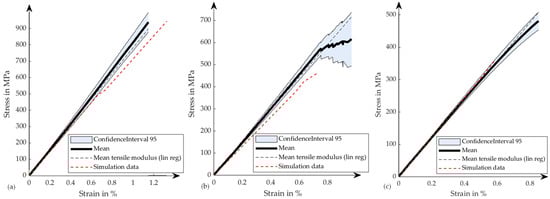
Figure 9.
Stress-strain curves of the different variation specifications: (a) 0° variation; (b) 5° variation; (c) 10° variation.
Analyzing the specification with 5° variations in Figure 9b good linear behavior with low variations until the first ply failure can be observed. The mean curve matches very good with the mean tensile modulus. In the area above 0.7 % strain first ply failures severely increases the variation and therefore is less informative. Differences in the calculated tensile modulus exist and are discussed in a later paragraph.
In Figure 9c the 10° specification shows good linear behavior for low strains. Above 0.5 % slightly nonlinear behavior can be observed with decreasing steepness, respectively tensile modulus. The confidence interval remains narrow until the nonlinearity increases. The results show consistent results with relatively small variations, indicating a high manufacturing quality.
In the next step the tensile modulus is determined directly from the stress-strain curves through the application of linear regression. Complementary to the mean stress-strain curves, the mean tensile modulus is depicted in Figure 9 as dashed black line Furthermore, the mean values and standard deviations are presented in Table 2. While the tensile modulus shows good fitting for lower strain values across all three specifications, for higher strain values small differences can be observed. The mean tensile modulus of the nominal specification slightly underestimates the tensile stiffness of the laminate in the mean stress-strain curve. Nevertheless, the mean tensile modulus lies within the confidence interval of the experiments. The variational specifications show good agreement of the mean tensile modulus until first ply failure (5° specification) and nonlinearity above 0.6% strain.
Table 2.
Mean and standard deviation values of the tensile modulus and tensile strength of three different variation specifications.
Furthermore, Table 2 shows the differences of the specifications. The 5° variation results in a minor decrease in the tensile modulus of −5.48%, whereas the 10° variations show a larger effect (−24.01%). All three specifications show acceptable standard deviations below 5% of the mean value. Despite the recognizable differences in the mean values of the tensile modulus, the question arises whether the tensile moduli of the three specifications differ significantly.
Therefore, the data is investigated using significance testing. A two-sided t-test is performed on the tensile moduli of all specimens of each specification. The hypothesis to be tested is that the tensile moduli of the different specification datasets are from different normal distributions and therefore have different sets of ply angles. The resulting null hypothesis which has to be rejected states that: The datasets are from the same distribution. The results of the two-sided t-test are listed in Table 3. The tests use two different significance levels, the common 5 % level and a less strict significance level of 10 %. The results show significant separation of the tensile moduli of the 0° and 10° as well as the 5° and 10° comparison at both levels. The comparison of the 0° and 5° is only significant at the 10% level, which leads to the conclusion that effects of small ply angle variations can only be observed with higher uncertainty. Further variations sources might overlay effects of ply angle variations.
Table 3.
Significance testing of the laminate tensile modulus with two-sided t-test and significance level alpha = 0.05 and alpha = 0.1.
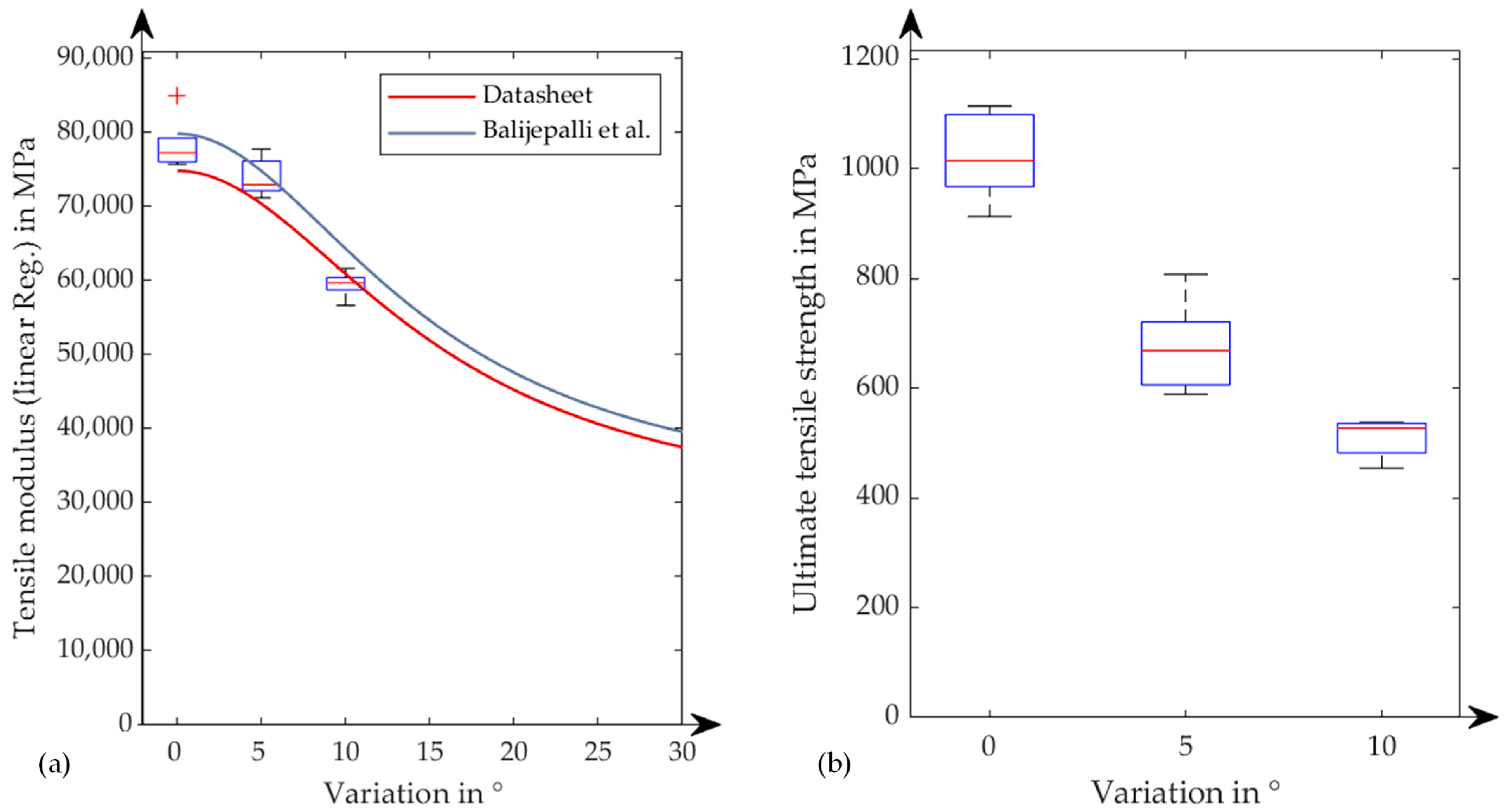
Additionally, the results for the tensile modulus of the three specifications are presented in Figure 10a as boxplots, complemented with the theoretical curves calculated analytically using classical laminate theory for the laminate based on the datasheet values of the material and the less conservative values from [37]. The challenges associated with significance testing while distinguishing the 0° and 5° specification can be observed as well. While the median values of both show different values, the boxes defined by the 25th and 75th percentile overlap and thereby complicate separating both specifications. Overall, all three specifications show a good fit with the theoretically assumed values. While the experimental data of the 0° and 5° specification lie between both curves, the 10° fits best with the datasheet values.
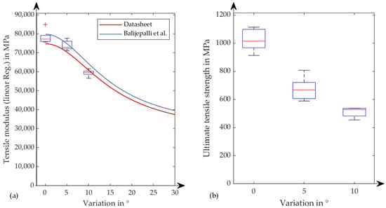
Figure 10.
Box plots of the tensile modulus (a) and ultimate tensile strength (b) of the three datasets. The tensile modulus is overlayed with the analytically calculated curves using the datasheet material values [33] and from [34].
Investigating the ultimate tensile strength Figure 8 already revealed considerable high variations of the failure force and deformation. The presented mean values and standard deviations of the ultimate tensile strength from Table 2 underline this observation. In particular, the variations for the 5° specification are quite high. The standard deviation is 12.7% of the mean value, while the other two specifications show values below 10%. The higher variations of the 5° specification can be explained by the occurrence of the first ply failures which do not lead directly to ultimate failure. Therefore, they lead to a high scatter of the engineering stresses used for failure analysis. Despite the high scatter in the strength values, the decrease in strength of −34.22% is remarkable. From the nominal 0° specification to the 10° specification a 50% loss in strength can be observed. In addition, Figure 10b shows the strength measurements as box plots. The critical decrease in the first degrees of variation slightly flattens with higher variations of the ply angles. Therefore, especially the part strength is strongly driven by small fiber angle variations. Analogous to the significance test for the tensile modulus of the specifications, significance tests were performed for ultimate tensile strength. The results in Table 4 confirm the observation of strongly different values. All tests show significance, meaning that the assumed normal distributions can be distinguished from the experimental data at a 5% significance level. Interestingly, the smaller difference between the mean values of the 5° and 10° specifications and the large variation of 5° specification lead to slightly worse values, especially for the power, which is a measure for the probability of a false negative result.
Table 4.
Significance testing of the ultimate tensile strength with two-sided t-test and significance level alpha = 0.05.
3.2. Material Calibration
The material calibration was performed according to Section 2.6 using the mean curves of the specifications as shown in Figure 9. The LS-Dyna simulation model is presented in Figure 11, supplemented by the results of all three specifications in the timestep prior to the beginning of failure. The datasheet values from are used as material data. The presented simulation models are used as the basis for the material calibration procedure, where the ply properties are calculated based on the experimental results of the laminate.
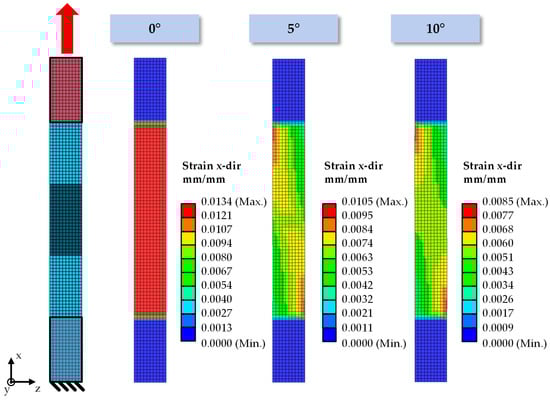
Figure 11.
LS Dyna simulation model on the left side, with restricted degrees in the bottom element set (light blue) and an applied displacement in x-direction while the remaining directions are constrained in the top set (red). The middle element set (dark blue) represents the area where the strains are measured in accordance to the experimental measurements; The right three figures show the simulation results for the three specifications in the timestep before first failure occurred.
First the calibration procedure was performed for the ply properties Ex, Ey, Gxy, vxy using the 0° specification. The optimized values are listed in Table 5. While the Young’s modulus in fiber direction x has higher values than the datasheet suggests and lies within the range of uncertainty published in [37], the other three ply properties show much smaller values than the datasheet values. The driving parameter behind the stress-strain curve for the tensile test is the Young’s modulus in fiber direction. Furthermore, effects resulting from the other parameters are not contained in the used stress-strain curves. The results show that the strain field follows the variations leading to asymmetry. Therefore, using the full strain field could improve the contained information and thus fitting.
Table 5.
Material properties of the Vorafuse TM P6300 from different sources.
To further improve the calibrated ply properties all three specifications are used during the calibration process. This creates a multi objective optimization problem which does not result in a single optimal solution, but in a Pareto front of solutions where changes in the design variables (ply parameters) would result in an equally good or worsened curve matching (objective value). By using the three specifications with the small variations in ply angles the resulting laminate stiffness changes and therefore the other ply parameters must be considered more intensively by the optimization algorithm to fit the curves best. This can also be seen in the results in Table 5, which shows the best solution from the Pareto front, i.e., the solution with the smallest summed curve matching errors at equal weights. The Young’s modulus in fiber direction Ex, shear modulus and Poisson’s ratio are close to the datasheet and published values. Only the Young’s modulus Ey is still lower than the reference data. Nonetheless, it increased compared to the calibration of the 0° specification.
3.3. Evaluation of Simulative Modeling of Variations
The resulting mechanical properties from calibration with the 0° specification are applied to the prepared simulation models. The resulting simulated stress-strain curves for all three specifications are depicted in Figure 9 as red dashed lines. For the 0° and 5° specifications the simulated stress-strain curves lie below the experimental results, underestimating the laminate stiffness. For the 10° specification the experimental and simulated results are in good agreement, which is additionally presented in Table 6.
Table 6.
Comparison of laminate tensile modulus in experiment and simulation.
Further improvements are achieved using the material properties calibrated with all three specifications. The corresponding stress-strain curves of the simulation are compared with the measured data in the Appendix A Figure A1. While the major part of the 0° simulation and 10° simulation curves are within the confidence intervals, experimental results for the 5° specification still show stiffer behavior than predicted by the simulation. Overall, the laminate tensile modulus improves for the 0° and 5° specifications.
4. Discussion
Investigating the effects of ply angle variations, i.e., fiber misalignment, on the structural behavior, the experiments show significant differences in the mechanical properties of the laminates. Artificial variations were introduced into the laminate using a tape laying machine. The variations studied are relatively small with variations of 5° and 10°, representing realistic variations from draping or manual lay-up or variations in the raw material. The effects of the variations can be detected in the form of a reduced tensile modulus of the laminate and strongly reduced strength values. While the effect of the 5° variation specification shows a moderate decrease of the tensile modulus, which is only significant with higher significance level, the decrease from 5°to 10° variation is more clear. Nevertheless, all experimental data are in good agreement with the predictions from laminate theory. The effects from small ply angle variations less than 5° are more difficult to extract from the experimental data because they overlap with other variations. Furthermore, the small dataset used for statistical testing complicates its evaluation.
Tensile strength of the laminate is strongly affected by the artificial variations. Even the small variations of 5° result in a significant reduction of strength. Additionally, the variations of the tensile strength are higher, so the effects of any variations (ply angles and others) are more critical.
The artificial variations can be well detected in laminate testing. The results show the strong influence on the strength and on the stiffness of the laminate and therefore underline the need for good quality and variations management during product development.
The standardized tensile test method was able to measure the changes in the structural behavior of the laminate. The results showed significant variations of strength and stiffness, which can be well extracted from the stress-strain curves. Nonetheless, using the tensile tests has some drawbacks. In the experiments presented, only variations of the plies parallel to the applied load were investigated. Since laminates are typically stacked from layers with different ply orientations, ply variations in the perpendicular direction have less influence and relevance in the testing results. Therefore, further tests in the perpendicular direction are needed to improve the quality of the results.
It is not possible to identify the cause of the variations solely based on the experimental stress-strain curves due to the limited information. Prestudies using an inverse approach to calculate the causing ply angle variations were not successful. The limited information in a single stress-strain curve is not sufficient to solve such an ill-posed problem where different solutions (variation sets) can lead to the same stress-strain curve respectively tensile modulus. However, with an increased amount of data for example using Digital Image Correlation (DIC) methods resulting in full-field strain data, additional spatial information on the spatial structural behavior becomes available, which improves the inverse characterization approach of the underlying variations. Future investigations using the complete strain field for variation characterization (and material property characterization) need to show the potential of the additional data.
The simulation results show good agreement with the experimental results using the material properties calibrated with the laminate tensile tests. Effects such as the small increase of tensile stiffness at higher strains are not considered in the simulation model. This means that using standardized test methods and the resulting stiffness, the simulation will fit best in the evaluated strain region. An extrapolation will result in higher errors.
The investigated loss of tensile stiffness resulting from ply orientation variations is detected in the experimental and simulation results as well. Especially, the 0° specification and 10° specification results match very well, while the simulation results of the 5° specification slightly underestimate the laminate’s tensile stiffness. Nonetheless, at low strains the simulation curve lies within the confidence interval. In general, the agreement of experimental and simulation data is good. Simulation can represent the effect of variations well. Therefore, the use of simulation tools for variation analysis is valid and allows a deeper understanding of variation effects due to high numbers of possible investigations, compared to experimental investigations.
5. Conclusions
Variations are inevitable in the manufacturing of composites parts. The variations result in changed laminate properties, influencing the structural performance of composite structures. Investigations on the effects of variations are essential for better predictability. In this contribution, the effects of small artificial variations were investigated regarding the tensile stiffness and strength of composite laminates. The resulting test data was used for significance testing the effects of the variations. Furthermore, based on the experimental data of the nominal and variational laminates, material property characterization was performed, which is used to replicate and compare the experimental results with simulation.
The results showed significant differences in the tensile properties of the laminate due to the variations. While tensile strength is very sensitive to even small variations, tensile stiffness decreases strongly for variations greater than 5°. For smaller variations, the decrease in tensile stiffness is small relative to the scatter. Additional variations e.g., in geometry, thickness, raw material, overlay the ply angle variations. To summarize the experimental results, the variations showed significant influence on the structural behavior, which needs to be considered in the design process. The effects of the variations could be recognized well in the results of the standardized test methods.
Based on the three specifications, a material calibration procedure was performed using the experimental results of the laminate and a simulation model. The optimization routine computed the best fitting material properties for the plies. However, due to the limited amount of data, the results should be interpreted with caution. Especially the material parameters perpendicular to the force direction have small contribution to the tensile stiffness and therefore cannot be computed precisely. While material calibration could be improved with additional tensile tests in the perpendicular direction, the simulation model matched well with the experimental results. Moreover, the simulation results showed the same decrease in tensile stiffness, but with slight differences in how well the single specifications can be represented. Overall, the simulation is able to represent the variations and can be used for further variation simulation.
This contribution highlights the need for good variation management in composite structures by investigating different small artificially induced fiber orientation variations that have a significant impact on the structural behavior. The simulation models used are capable to reproduce the effects seen in the experimental results. Therefore, they can be used for detailed variation analyses, helping product developers to tackle the challenges of variations within the development phase, for example by defining tolerances or improved manufacturing process design to increase the quality of composite products.
Author Contributions
Conceptualization, M.F., B.E., R.R. and S.W.; methodology, M.F.; software, M.F.; validation, M.F. and R.R.; formal analysis, M.F.; investigation, M.F.; resources, R.R. and B.E.; data curation, M.F.; writing—original draft preparation, M.F. and R.R.; writing—review and editing, M.F., R.R., B.E. and S.W.; visualization, M.F.; supervision, B.E. and S.W.; funding acquisition, S.W. All authors have read and agreed to the published version of the manuscript.
Funding
This research was funded by Bayerische Forschungsstiftung within the program for the initiation of international cooperations BayIntAn, grant number Bay_Int_An_FAU_2022_88. The authors gratefully thank Bayerische Forschungsstiftung for the funding.
Data Availability Statement
The data is available from the authors upon reasonable request.
Conflicts of Interest
The authors declare no conflict of interest.
Appendix A
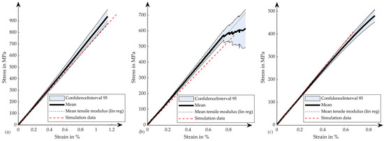
Figure A1.
Stress-strain curves of the different variation specifications: (a) 0° variation; (b) 5° variation; (c) 10° variation compared to the simulation data using the material properties calibrated with three specifications.
Figure A1.
Stress-strain curves of the different variation specifications: (a) 0° variation; (b) 5° variation; (c) 10° variation compared to the simulation data using the material properties calibrated with three specifications.
References
- Völkl, H.; Franz, M.; Wartzack, S. A Case Study on Established and New Approaches for Optimized Laminate Design. In Proceedings of the ECCM18—18th European Conference on Composite Materials, Athens, Greece, 25–28 June 2018; pp. 1–8. [Google Scholar]
- Kussmaul, R.; Jónasson, J.G.; Zogg, M.; Ermanni, P. A novel computational framework for structural optimization with patched laminates. Struct. Multidisc Optim. 2019, 60, 2073–2091. [Google Scholar] [CrossRef]
- Chai, B.; Eisenbart, B.; Nikzad, M.; Fox, B.; Blythe, A.; Blanchard, P.; Dahl, J. Simulation-based optimisation for injection configuration design of liquid composite moulding processes: A review. Compos. Part A Appl. Sci. Manuf. 2021, 149, 106540. [Google Scholar] [CrossRef]
- Taguchi, G.; Chowdhury, S.; Wu, Y. Taguchi’s Quality Engineering Handbook; John Wiley & Sons: Hoboken, NJ, USA; ASI Consulting Group: Livonia, MI, USA, 2005. [Google Scholar]
- AVK—Industrievereinigung Verstärkte Kunststoffe e. V. Handbuch Faserverbundkunststoffe, 4th ed.; Springer Fachmedien Wiesbaden: Wiesbaden, Germany, 2013.
- Mesogitis, T.S.; Skordos, A.A.; Long, A.C. Stochastic simulation of the influence of fibre path variability on the formation of residual stress and shape distortion. Polym. Compos. 2017, 38, 2642–2652. [Google Scholar] [CrossRef]
- Talreja, R. 5—Manufacturing defects in composites and their effects on performance. In Polymer Composites in the Aerospace Industry; Irving, P., Soutis, C., Eds.; WP, Woodhead Publ./Elsevier: Amsterdam, The Netherlands, 2015; pp. 99–113. [Google Scholar]
- Potter, K.D. Understanding the origins of defects and variability in composites manufacture. In Proceedings of the International Conference on Composite Materials (ICCM)-17, Edinburgh, UK, 27–31 July 2009; p. 18. [Google Scholar]
- Chai, B.; Eisenbart, B.; Nikzad, M.; Fox, B.; Blythe, A.; Blanchard, P.; Dahl, J. A novel heuristic optimisation framework for radial injection configuration for the resin transfer moulding process. Compos. Part A Appl. Sci. Manuf. 2023, 165, 107352. [Google Scholar] [CrossRef]
- Fernström, V.; Lööf, J.; Frampton, A.; Brunnacker, L.; Wärmefjord, K.; Söderberg, R. Variation Analysis of Carbon Fibre Reinforced Polymers Light Weight Aero Engine Parts. In Proceedings of the ASME 2022 International Mechanical Engineering Congress and Exposition. Volume 2B: Advanced Manufacturing, Columbus, OH, USA, 30 October–3 November 2022. V02BT02A071. ASME. [Google Scholar] [CrossRef]
- Potter, K.; Khan, B.; Wisnom, M.; Bell, T.; Stevens, J. Variability, fibre waviness and misalignment in the determination of the properties of composite materials and structures. Compos. Part A Appl. Sci. Manuf. 2008, 39, 1343–1354. [Google Scholar] [CrossRef]
- Toyoda, D.; Wärmefjord, K.; Söderberg, R. Challenges in geometry assurance for composites manufacturing. J. Comput. Inf. Sci. Eng. 2023, 23, 051007. [Google Scholar] [CrossRef]
- Corrado, A.; Polini, W. Analysis of process-induced deformation on the spring-in of carbon fiber-reinforced polymer thin laminates. J. Compos. Mater. 2019, 53, 2901–2907. [Google Scholar] [CrossRef]
- Jensen, E.M.; Leonhardt, D.A.; Fertig, R.S. Effects of thickness and fiber volume fraction variations on strain field inhomogeneity. Compos. Part A Appl. Sci. Manuf. 2015, 69, 178–185. [Google Scholar] [CrossRef]
- Franz, M.; Schleich, B.; Wartzack, S. Tolerance management during the design of composite structures considering variations in design parameters. Int. J. Adv. Manuf. Technol. 2021, 204, 359. [Google Scholar] [CrossRef]
- Jareteg, C.; Wärmefjord, K.; Söderberg, R.; Lindkvist, L.; Carlson, J.; Cromvik, C.; Edelvik, F. Variation Simulation for Composite Parts and Assemblies Including Variation in Fiber Orientation and Thickness. Procedia. CIRP 2014, 23, 235–240. [Google Scholar] [CrossRef]
- Kunze, E.; Galkin, S.; Böhm, R.; Gude, M.; Kärger, L. The Impact of Draping Effects on the Stiffness and Failure Behavior of Unidirectional Non-Crimp Fabric Fiber Reinforced Composites. Materials 2020, 13, 2959. [Google Scholar] [CrossRef] [PubMed]
- Söderberg, R.; Wärmefjord, K.; Lindkvist, L. Variation simulation of stress during assembly of composite parts. CIRP Annals 2015, 64, 17–20. [Google Scholar] [CrossRef]
- Chai, B.X.; Eisenbart, B.; Nikzad, M.; Fox, B.; Wang, Y.; Bwar, K.H.; Zhang, K. Review of Approaches to Minimise the Cost of Simulation-Based Optimisation for Liquid Composite Moulding Processes. Materials 2023, 16, 7580. [Google Scholar] [CrossRef]
- Yurgartis, S.W. Measurement of small angle fiber misalignments in continuous fiber composites. Compos. Sci. Technol. 1987, 30, 279–293. [Google Scholar] [CrossRef]
- Wang, B.; Zhong, S.; Lee, T.-L.; Fancey, K.S.; Mi, J. Non-destructive testing and evaluation of composite materials/structures: A state-of-the-art review. Adv. Mech. Eng. 2020, 12, 168781402091376. [Google Scholar] [CrossRef]
- Tucker, C.L., III. Fundamentals of Fiber Orientation: Description, Measurement and Prediction; Hanser Publishers: Munich, Germany, 2022. [Google Scholar]
- ASTM E2533-21; Standard Guide for Nondestructive Examination of Polymer Matrix Composites Used in Aerospace Applications. ASTM International: West Conshohocken, PA, USA, 2021.
- ASTM D3039; Test Method for Tensile Properties of Polymer Matrix Composite Materials. ASTM International: West Conshohocken, PA, USA, 2002.
- ISO 527-1:2019; Plastics—Determination of Tensile Properties—Part 1: General principles. ISO: Geneva, Switzerland, 2019.
- Wang, H.; Zhou, H.; Gui, L.; Ji, H.; Zhang, X. Analysis of effect of fiber orientation on Young’s modulus for unidirectional fiber reinforced composites. Compos. Part B Eng. 2014, 56, 733–739. [Google Scholar] [CrossRef]
- Sarangapani, G.; Ganguli, R. Effect of Ply-Level Material Uncertainty on Composite Elastic Couplings in Laminated Plates. Int. J. Comput. Methods Eng. Sci. Mech. 2013, 14, 244–261. [Google Scholar] [CrossRef]
- Patel, H.V.; Dave, H.K. Effect of fiber orientation on tensile strength of thin composites. Mater. Today Proc. 2021, 46, 8634–8638. [Google Scholar] [CrossRef]
- Fedulov, B.; Antonov, F.; Safonov, A.; Ushakov, A.; Lomov, S. Influence of fibre misalignment and voids on composite laminate strength. J. Compos. Mater. 2015, 49, 2887–2896. [Google Scholar] [CrossRef]
- Dey, S.; Mukhopadhyay, T.; Adhikari, S. Uncertainty Quantification in Laminated Composites; CRC Press, Taylor & Francis Group, [2018]|“A Science Publishers Book”; CRC Press: Boca Raton, FL, USA, 2018. [Google Scholar]
- Schwer, L.E. An overview of the ASME V&V-10 guide for verification and validation in computational solid mechanics. In Proceedings of the 20th International Conference on Structural Mechanics in Reactor Technology, Espoo, Finland, 9–14 August 2009; pp. 1–10. [Google Scholar]
- ISO 527-4:2019; Plastics—Determination of tensile properties—Part 4: Test Conditions for Isotropic and Orthotropic Fibre-Reinforced Plastic Composites. ISO: Geneva, Switzerland, 2020.
- Sutcliffe, M.P.F.; Lemanski, S.L.; Scott, A.E. Measurement of fibre waviness in industrial composite components. Compos. Sci. Technol. 2012, 72, 2016–2023. [Google Scholar] [CrossRef]
- Toft, H.S.; Branner, K.; Mishnaevsky, L.; Sørensen, J.D. Uncertainty modelling and code calibration for composite materials. J. Compos. Mater. 2013, 47, 1729–1747. [Google Scholar] [CrossRef]
- Chang, F.-K.; Chang, K.-Y. A Progressive Damage Model for Laminated Composites Containing Stress Concentrations. J. Compos. Mater. 1987, 21, 834–855. [Google Scholar] [CrossRef]
- VORAFUSE™ Epoxy Intermediates for Pre-preg Solutions. 2018.
- Balijepalli, B.; Bank, D.; Lowe, M.; Ma, L.; James, A.; Baumer, R. High quality carbon fiber epoxy prepregs for a wide range of reinforcement architectures. In Proceedings of the SPE ACCE: Opportunities & Challenges with Carbon Composites + Carbon Composites. SPE ACCE 2017: Society of Plastic Engineers (SPE) and Automotive Composites Conference Exhibition (ACCE) 2017 Conference, Novi, MI, USA, 6–8 September 2017. [Google Scholar]


Disclaimer/Publisher’s Note: The statements, opinions and data contained in all publications are solely those of the individual author(s) and contributor(s) and not of MDPI and/or the editor(s). MDPI and/or the editor(s) disclaim responsibility for any injury to people or property resulting from any ideas, methods, instructions or products referred to in the content. |
© 2024 by the authors. Licensee MDPI, Basel, Switzerland. This article is an open access article distributed under the terms and conditions of the Creative Commons Attribution (CC BY) license (https://creativecommons.org/licenses/by/4.0/).