
A Refinement of Backward Correlation Technique for Precise Brillouin Frequency Shift Extraction


Abstract
1. Introduction
2. Methodology
- (1)
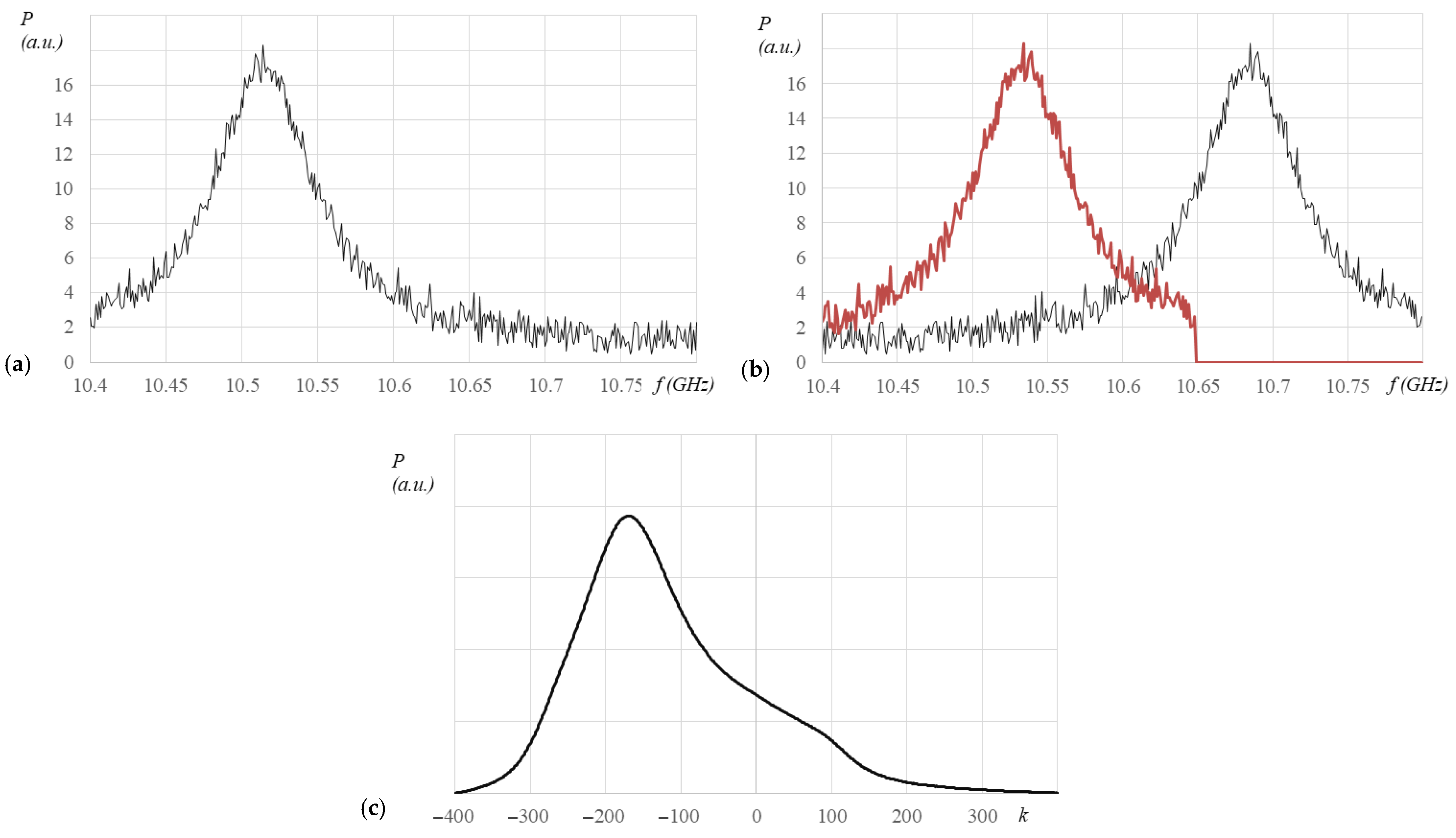
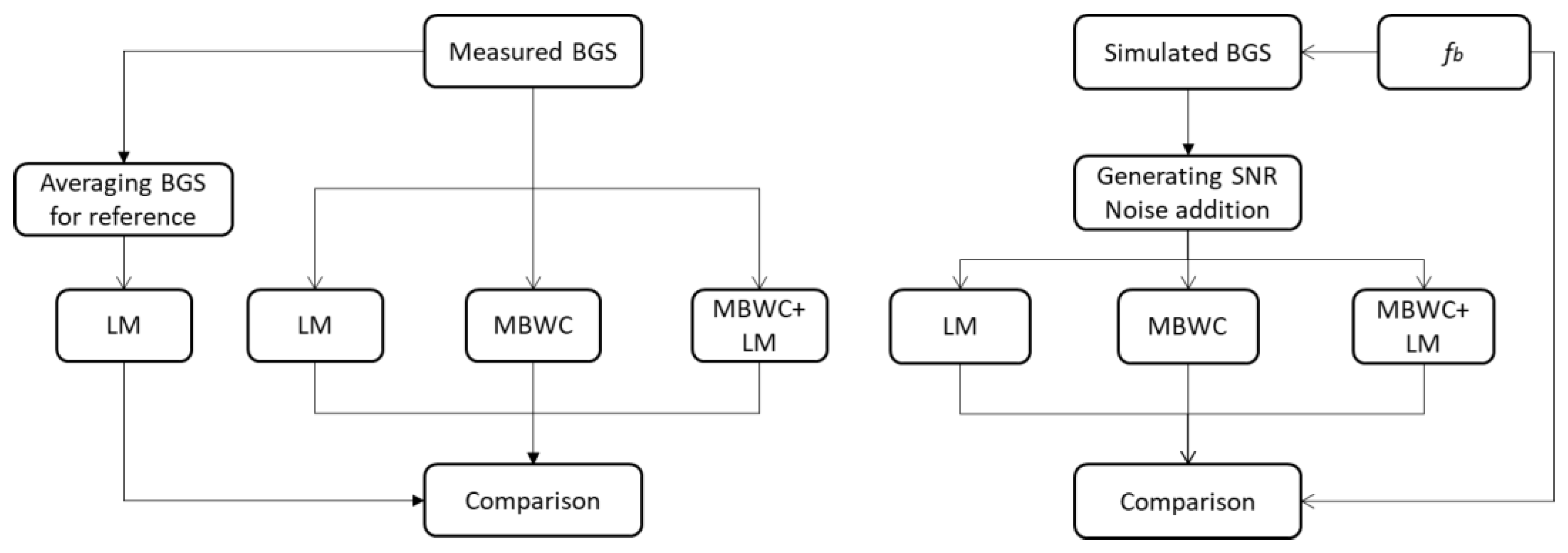
- Calculate the average value R of the power spectral density over the entire spectrum. Since it is equal to the sum of the average value of the useful signal S and the average value of the side signal N, it will certainly be higher than N.
- (2)
- The test value for subtracting Q is set to R.
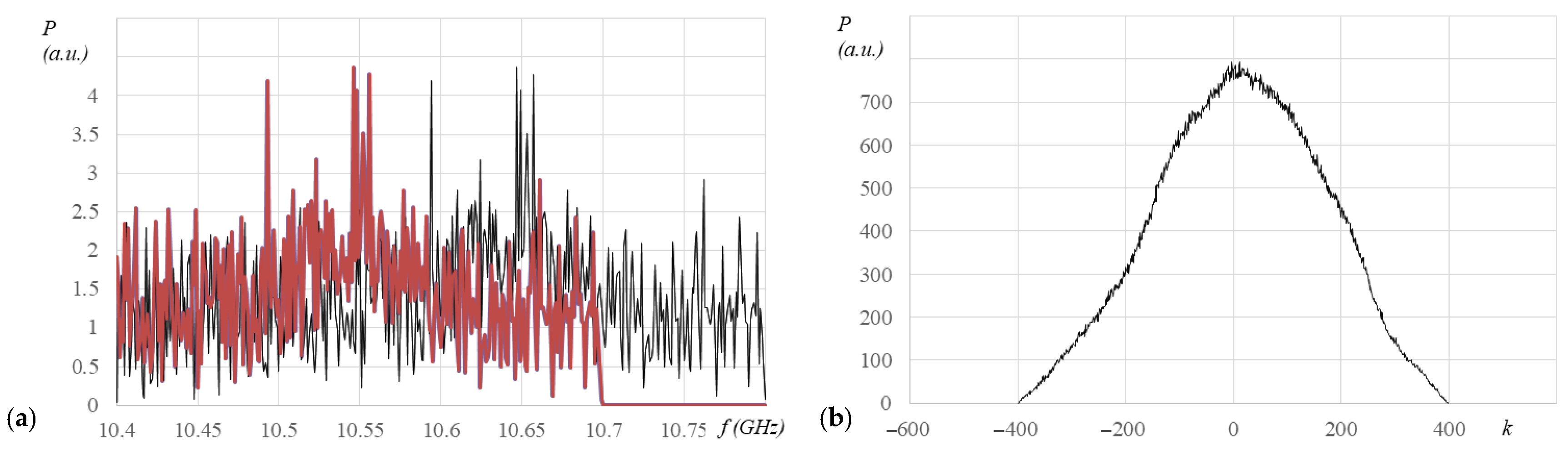
- (3)
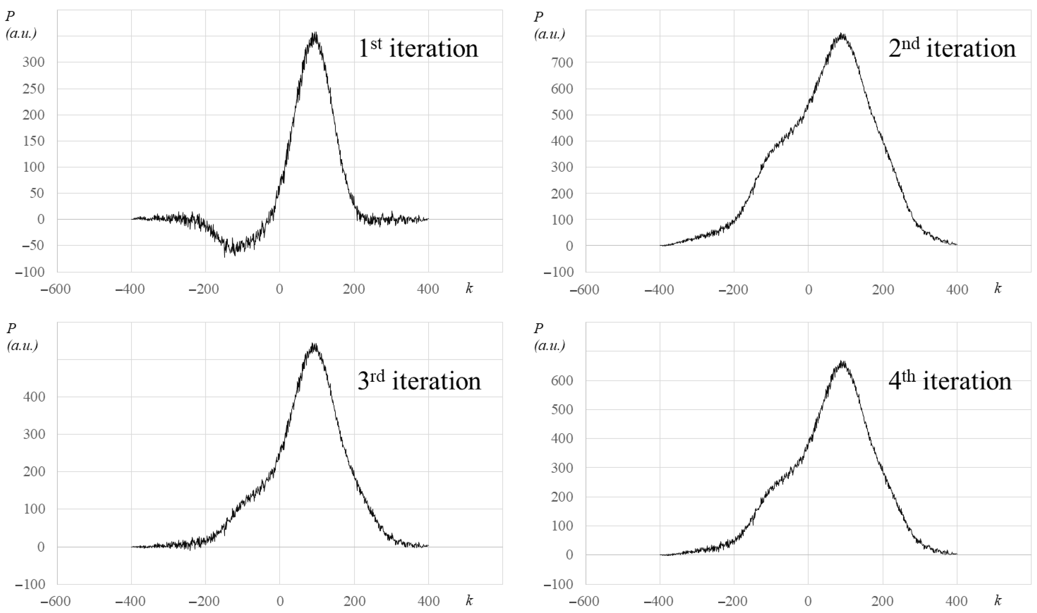
- The value of Q is subtracted from all points of the spectrum, and a correlogram is constructed. During the construction, the number of the resulting function negative values is counted.
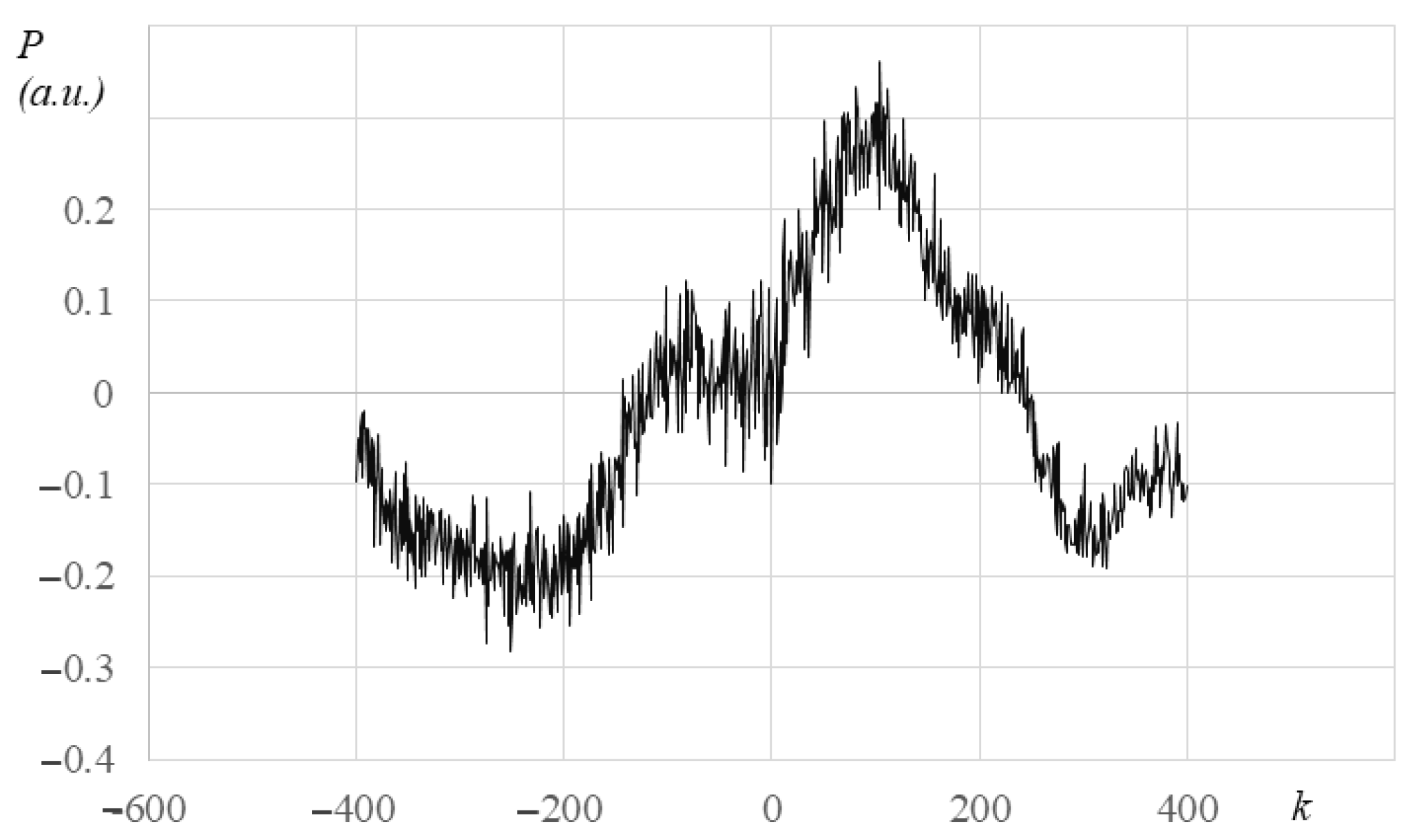
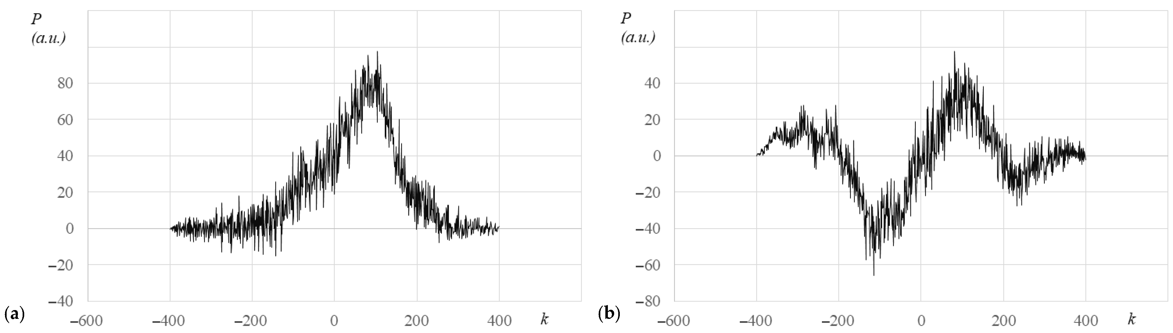
- (4)
- If there are no negative values (we received a correlogram as in Figure 2), then the subtracted value was insufficient. If there are too many negative values (we have a correlogram as in Figure 4B), then we subtract excessively. In both cases, we proceed to step 5.Otherwise, we consider that we have subtracted the desired value and exited the loop. Since the real correlogram always has some noise, in practice, the loop was excited when more than 1% and less than 5% of the correlogram points fell into the negative region.
- (5)
- Q value is corrected by the method of half division of the segment [0,R], and we go back to step 3.
3. Simulation
4. Experiment
5. Results and Discussion
6. Summary
Author Contributions
Funding
Data Availability Statement
Acknowledgments
Conflicts of Interest
References
- Gharehbaghi, V.R.; Noroozinejad Farsangi, E.; Noori, M.; Yang, T.Y.; Shaofan, L.; Nguyen, A.; Málaga-Chuquitaype, C.; Gardoni, P.; Mirjalili, S. A Critical Review on Structural Health Monitoring: Definitions, Methods, and Perspectives. Arch. Comput. Methods Eng. 2022, 29, 2209–2235. [Google Scholar] [CrossRef]
- Peng, J.; Lu, Y.; Zhang, Z.; Wu, Z.; Zhang, Y. Distributed Temperature and Strain Measurement Based on Brillouin Gain Spectrum and Brillouin Beat Spectrum. IEEE Photonics Technol. Lett. 2021, 33, 1217–1220. [Google Scholar] [CrossRef]
- Stepanov, K.V.; Zhirnov, A.A.; Koshelev, K.I.; Chernutsky, A.O.; Khan, R.I.; Pnev, A.B. Sensitivity Improvement of Phi-OTDR by Fiber Cable Coils. Sensors 2021, 21, 7077. [Google Scholar] [CrossRef]
- Gui, X.; Li, Z.-Y.; Wang, H.-H.; He, J.; Hu, C.-C.; Ma, L.-J.; Lou, Z. Research on Distributed Gas Detection Based on Hollow-core Photonic Crystal Fiber. Sens. Transducers 2014, 174, 14–20. [Google Scholar]
- Bao, Y.; Huang, Y.; Hoehler, M.S.; Chen, G. Review of Fiber Optic Sensors for Structural Fire Engineering. Sensors 2019, 19, 877. [Google Scholar] [CrossRef]
- Agliullin, T.; Anfinogentov, V.; Morozov, O.; Sakhabutdinov, A.; Valeev, B.; Niyazgulyeva, A.; Garovov, Y. Comparative Analysis of the Methods for Fiber Bragg Structures Spectrum Modeling. Algorithms 2023, 16, 101. [Google Scholar] [CrossRef]
- Liokumovich, L.B.; Ushakov, N.A.; Kotov, O.I.; Bisyarin, M.A.; Hartog, A.H. Fundamentals of Optical Fiber Sensing Schemes Based on Coherent Optical Time Domain Reflectometry: Signal Model Under Static Fiber Conditions. J. Light. Technol. 2015, 33, 3660–3671. [Google Scholar] [CrossRef]
- Tkachenko, A.Y.; Lobach, I.A.; Kablukov, S.I. Coherent optical frequency reflectometer based on a fibre laser with self-scanning frequency. Quantum Electron. 2019, 49, 1121. [Google Scholar] [CrossRef]
- Wu, Y.; Wang, Z.; Xiong, J.; Jiang, J.; Lin, S.; Chen, Y. Interference Fading Elimination With Single Rectangular Pulse in Φ-OTDR. J. Light. Technol. 2019, 37, 3381–3387. [Google Scholar] [CrossRef]
- Zhao, Z.; Dang, Y.; Tang, M. Advances in Multicore Fiber Grating Sensors. Photonics 2022, 9, 381. [Google Scholar] [CrossRef]
- Matveenko, V.; Kosheleva, N.; Serovaev, G.; Fedorov, A. Measurement of Gradient Strain Fields with Fiber-Optic Sensors. Sensors 2023, 23, 410. [Google Scholar] [CrossRef] [PubMed]
- Sanchez, J.; Muñoz, O.; Russo, B.; Acero-Oliete, A.; Paindelli, A. Distributed temperature sensors system. Field Tests Earth Dam 2022, 6, 1–11. [Google Scholar] [CrossRef]
- Bogachkov, I.V.; Gorlov, N.I. Research of the Optical Fibers Structure Influence on the Acousto-Optic Interaction Characteristics and the Brillouin Scattering Spectrum Profile. J. Phys. Conf. Ser. 2022, 2182, 012088. [Google Scholar] [CrossRef]
- Zan, M.S.D.; Almoosa, A.S.K.; Mohd, F.I.; Elgaud, M.M.; Hamzah, A.E.; Arsad, N.; Mokhtar, M.H.H.; Bakar, A.A.A. The effect of pulse duration on the Brillouin frequency shift accuracy in the differential cross-spectrum BOTDR (DCS-BOTDR) fiber sensor. Opt. Fiber Technol. 2022, 72, 102977. [Google Scholar] [CrossRef]
- Li, M.; Xu, T.; Wang, S.; Hu, W.; Jiang, J.; Liu, T. Probe pulse design in Brillouin optical time domain reflectometry. IET Optoelectron. 2022, 16, 238–252. [Google Scholar] [CrossRef]
- Guo, Z.; Yan, J.; Han, G.; Yu, Y.; Greenwood, D.; Marco, J. High-resolution Φ-OFDR using phase unwrap and nonlinearity suppression. J. Light. Technol. 2023, 41, 2885–2891. [Google Scholar] [CrossRef]
- Zhao, S.; Cui, J.; Tan, J. Nonlinearity Correction in OFDR System Using a Zero-Crossing Detection-Based Clock and Self-Reference. Sensors 2019, 19, 3660. [Google Scholar] [CrossRef] [PubMed]
- Gorshkov, B.G.; Taranov, M.A. Simultaneous optical fibre strain and temperature measurements in a hybrid distributed sensor based on Rayleigh and Raman scattering. Quantum Electron. 2018, 48, 184. [Google Scholar] [CrossRef]
- Bai, Q.; Wang, Q.; Wang, D.; Wang, Y.; Gao, Y.; Zhang, H.; Zhang, M.; Jin, B. Recent Advances in Brillouin Optical Time Domain Reflectometry. Sensors 2019, 19, 1862. [Google Scholar] [CrossRef]
- Krivosheev, A.I.; Barkov, F.L.; Konstantinov, Y.A.; Belokrylov, M.E. State-of-the-Art Methods for Determining the Frequency Shift of Brillouin Scattering in Fiber-Optic Metrology and Sensing (Review). Instrum. Exp. Tech. 2022, 65, 687–710. [Google Scholar] [CrossRef]
- Haneef, S.M.; Yang, Z.; Thévenaz, L.; Venkitesh, D.; Srinivasan, B. Performance analysis of frequency shift estimation techniques in Brillouin distributed fiber sensors. Opt. Express 2018, 26, 14661–14677. [Google Scholar] [CrossRef]
- Nordin, N.D.; Zan, M.S.D.; Abdullah, F. Comparative Analysis on the Deployment of Machine Learning Algorithms in the Distributed Brillouin Optical Time Domain Analysis (BOTDA) Fiber Sensor. Photonics 2020, 7, 79. [Google Scholar] [CrossRef]
- Nordin, N.D.; Abdullah, F.; Zan, M.S.D.; Bakar, A.A.A.; Krivosheev, A.I.; Barkov, F.L.; Konstantinov, Y.A. Improving Prediction Accuracy and Extraction Precision of Frequency Shift from Low-SNR Brillouin Gain Spectra in Distributed Structural Health Monitoring. Sensors 2022, 22, 2677. [Google Scholar] [CrossRef] [PubMed]
- Barkov, F.L.; Konstantinov, Y.A.; Krivosheev, A.I. A Novel Method of Spectra Processing for Brillouin Optical Time Domain Reflectometry. Fibers 2020, 8, 60. [Google Scholar] [CrossRef]
- Barkov, F.L.; Konstantinov, Y.A. A modification of the backward correlation method for the brillouin frequency shift accurate extraction. Instrum. Exp. Tech. 2023, accepted. [Google Scholar]
- Li, C.; Li, Y. Fitting of Brillouin Spectrum Based on LabVIEW. In Proceedings of the 2009 5th International Conference on Wireless Communications, Networking and Mobile Computing, Beijing, China, 24–26 September 2009. [Google Scholar]
- Lourakis, M.L.; Argyros, A.A. Is Levenberg-Marquardt the most efficient optimization algorithm for implementing bundle adjustment? In Proceedings of the 10th IEEE International Conference on Computer Vision (ICCV), Beijing, China, 17–21 October 2005; Volume 2, p. 1526. [Google Scholar]
- Soto, M.A.; Thévenaz, L. Modeling and evaluating the performance of Brillouin distributed optical fiber sensors. Opt. Express 2013, 21, 31347–31366. [Google Scholar] [CrossRef]
- Qu, S.; Qin, Z.; Xu, Y.; Cong, Z.; Wang, Z.; Liu, Z. Improvement of Strain Measurement Range via Image Processing Methods in OFDR System. J. Light. Technol. 2021, 39, 6340–6347. [Google Scholar] [CrossRef]
- Qu, S.; Qin, Z.; Xu, Y.; Cong, Z.; Wang, Z.; Yang, W.; Liu, Z. High Spatial Resolution Investigation of OFDR Based on Image Denoising Methods. IEEE Sens. J. 2021, 21, 18871–18876. [Google Scholar] [CrossRef]
- Zhao, S.; Cui, J.; Wu, Z.; Tan, J. Accuracy improvement in OFDR-based distributed sensing system by image processing. Opt. Lasers Eng. 2020, 124, 105824. [Google Scholar] [CrossRef]
- Pan, M.; Hua, P.; Ding, Z.; Zhu, D.; Liu, K.; Jiang, J.; Wang, C.; Guo, H.; Teng, Z.; Li, S.; et al. Long Distance Distributed Strain Sensing in OFDR by BM3D-SAPCA Image Denoising. J. Light. Technol. 2022, 40, 7952–7960. [Google Scholar] [CrossRef]
- Wang, Q.; Zhao, K.; Badar, M.; Yi, X.; Lu, P.; Buric, M.; Mao, Z.-H.; Chen, K. Improving OFDR Distributed Fiber Sensing by Fibers With Enhanced Rayleigh Backscattering and Image Processing. IEEE Sens. J. 2022, 22, 18471–18478. [Google Scholar] [CrossRef]
- Qian, X.; Wang, Z.; Wang, S.; Xue, N.; Sun, W.; Zhang, L.; Zhang, B.; Rao, Y. 157km BOTDA with pulse coding and image processing. In Proceedings of the SPIE 9916, Sixth European Workshop on Optical Fibre Sensors, Limerick, Ireland, 31 May–3 June 2016; p. 99162S. [Google Scholar] [CrossRef]
- Yang, Y.; Liu, L.; Deng, Q.; Jia, X.; Wu, H.; Liang, W.; Jiang, L.; Song, W.; Ma, H.; Lin, J.; et al. Towards fast sensing along ultralong BOTDA: Flatness enhancement by utilizing injection-locked dual-bandwidth probe wave. Opt. Express 2022, 30, 20501–20514. [Google Scholar] [CrossRef]
- Wu, H.; Wan, Y.; Tang, M.; Chen, Y.; Zhao, C.; Liao, R.; Chang, Y.; Fu, S.; Shum, P.P.; Liu, D. Real-Time Denoising of Brillouin Optical Time Domain Analyzer With High Data Fidelity Using Convolutional Neural Networks. J. Light. Technol. 2019, 37, 2648–2653. [Google Scholar] [CrossRef]
- Azad, A.K.; Wang, L.; Guo, N.; Tam, H.Y.; Lu, C. Signal processing using artificial neural network for BOTDA sensor system. Opt. Express 2016, 24, 6769–6782. [Google Scholar] [CrossRef] [PubMed]
- Wang, B.; Wang, L.; Guo, N.; Zhao, Z.; Yu, C.; Lu, C. Deep neural networks assisted BOTDA for simultaneous temperature and strain measurement with enhanced accuracy. Opt. Express 2019, 27, 2530–2543. [Google Scholar] [CrossRef]
- Lv, T.; Ye, X.; Huang, K.; Zheng, Y.; Ge, Z.; Xu, Z.; Sun, X. Cascaded Feedforward Neural Network Based Simultaneously Fast and Precise Multi-Characteristics Extraction and BFS Error Estimation. J. Light. Technol. 2022, 40, 7937–7945. [Google Scholar] [CrossRef]
- Ruiz-Lombera, R.; Fuentes, A.; Rodriguez-Cobo, L.; Lopez-Higuera, J.M.; Mirapeix, J. Simultaneous Temperature and Strain Discrimination in a Conventional BOTDA via Artificial Neural Networks. J. Light. Technol. 2018, 36, 2114–2121. [Google Scholar] [CrossRef]
- Li, B.; Jiang, N.; Han, X. Denoising of BOTDR Dynamic Strain Measurement Using Convolutional Neural Networks. Sensors 2023, 23, 1764. [Google Scholar] [CrossRef]
- Chen, B.; Su, L.; Liu, X.; Zhang, Z.; Song, M.; Wang, Y.; Yang, J. Fast and high-accuracy temperature extraction of BOTDR sensor based on wavelet convolutional neural network. In Proceedings of the Eighth Symposium on Novel Photoelectronic Detection Technology and Applications, Kunming, China, 9–11 November 2021; p. 12169. [Google Scholar] [CrossRef]
- Krivosheev, A.I.; Konstantinov, Y.A.; Krishtop, V.V.; Turov, A.T.; Barkov, F.L.; Zhirnov, A.A.; Garin, E.O.; Pnev, A.B. A Neural Network Method for the BFS Extraction. In Proceedings of the 2022 International Conference Laser Optics (ICLO), St. Peters-burg, Russia, 20–24 June 2022. [Google Scholar] [CrossRef]


| Method/Parameter | BWC (Single) | MBWC (Single) | LM (Single) | MBWC + LM |
|---|---|---|---|---|
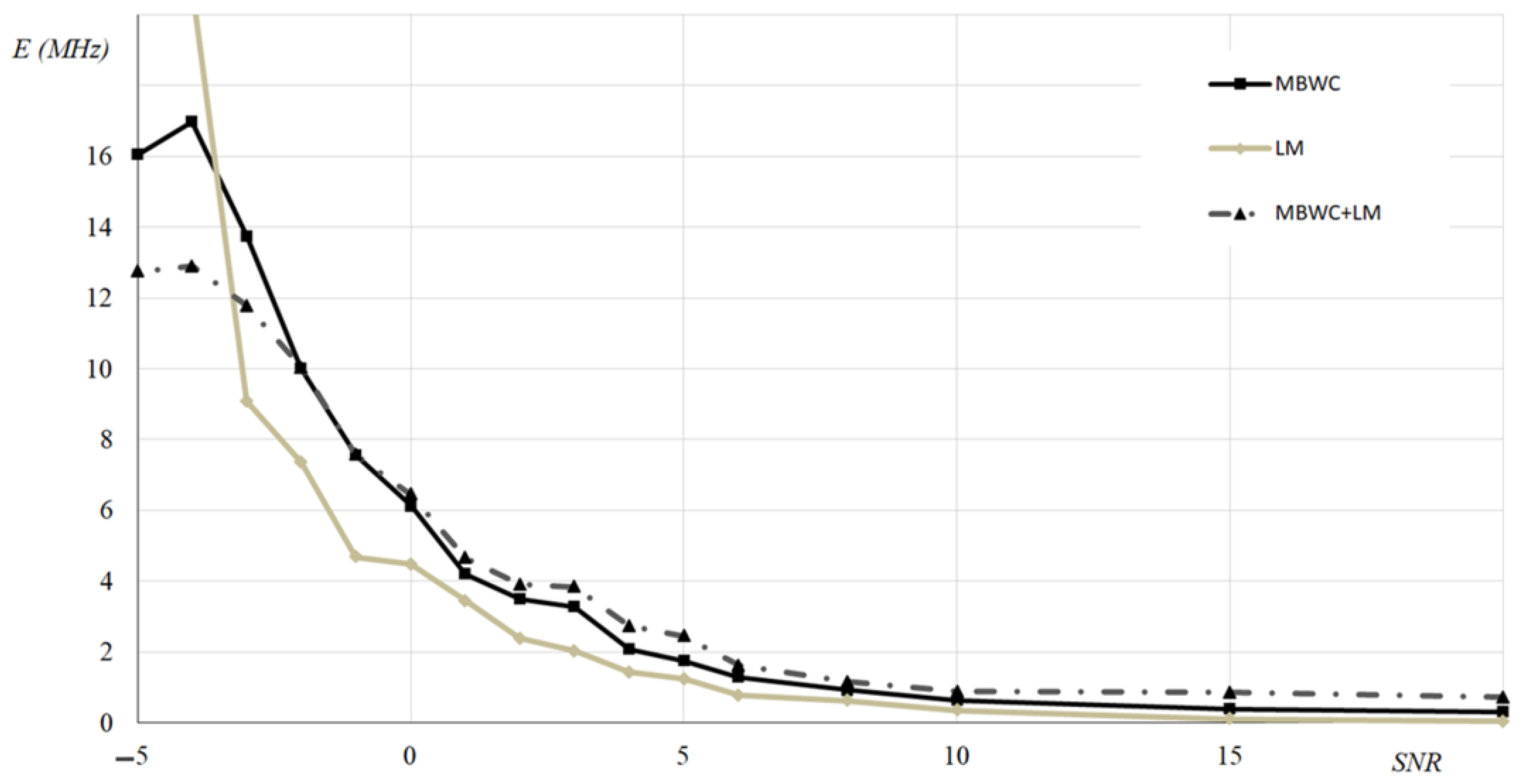
| Case 1 (201 point simulation) error at 0 dB SNR | 24.9 | 6.12 | 4.48 | 6.46 |
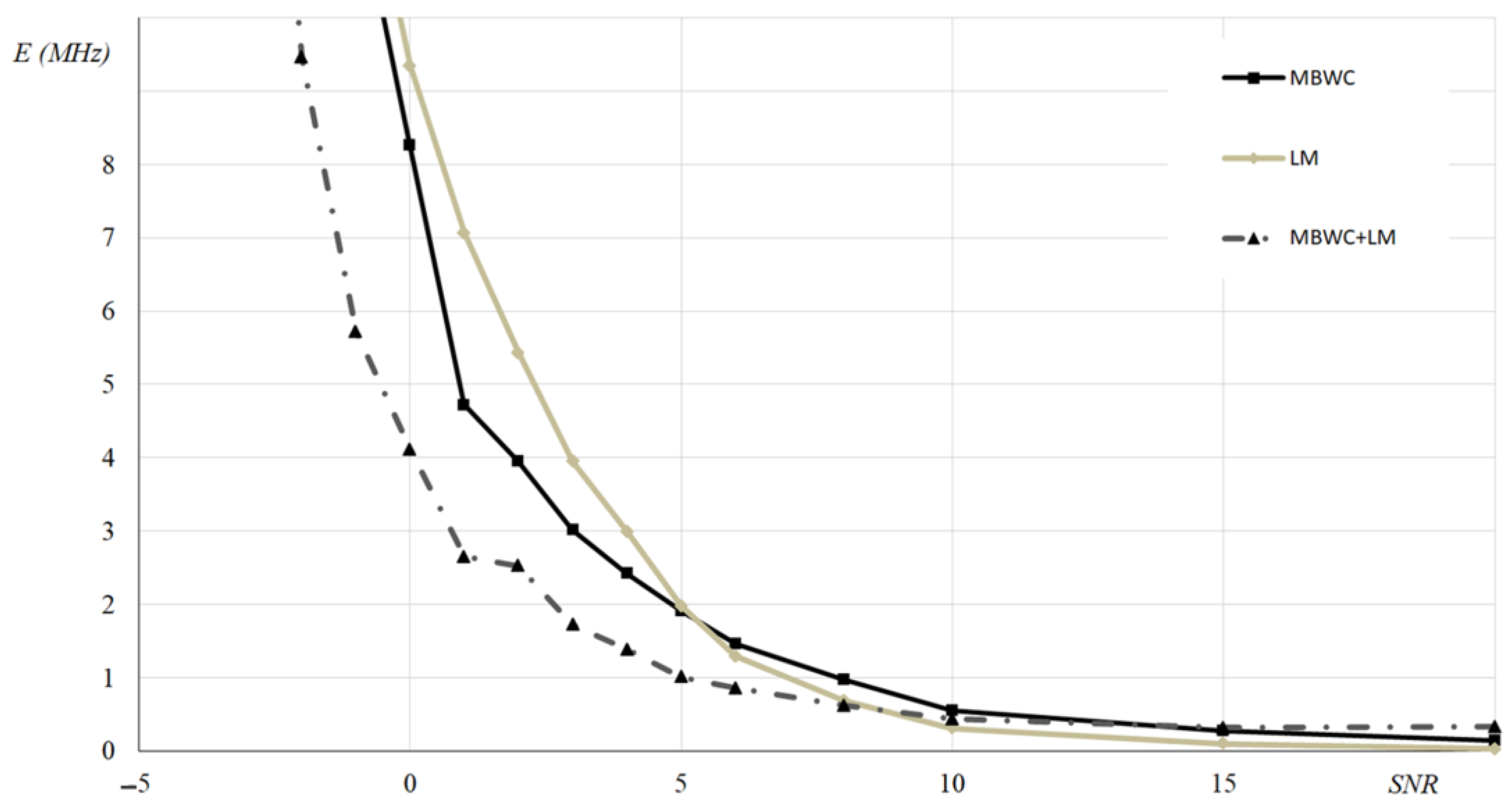
| Case 2 (401 point simulation) error at 0 dB SNR | 24.7 | 8.27 | 9.34 | 4.12 |
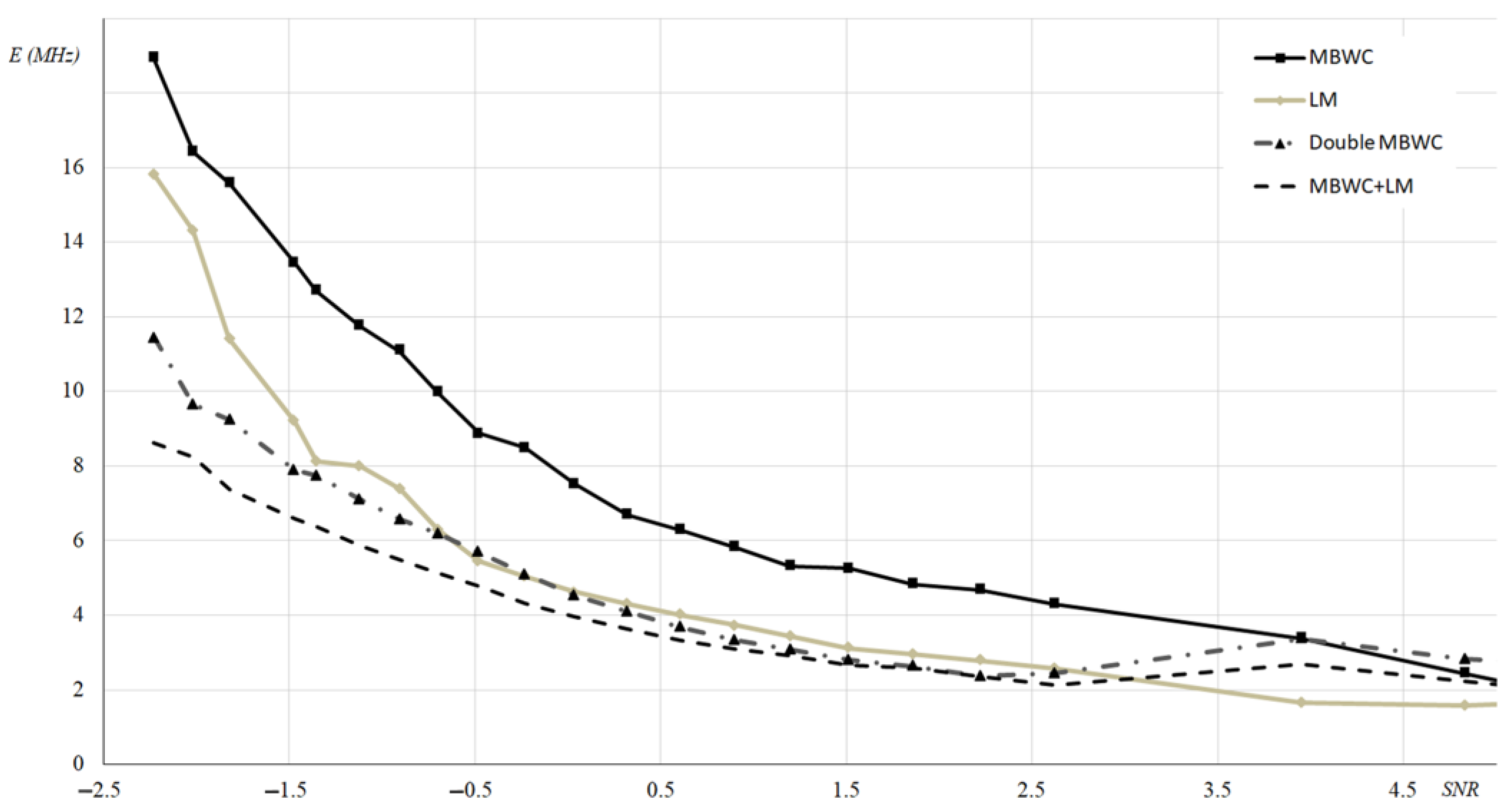
| Case 3 (experimental) error at 0 dB SNR | 19.5 | 7.53 | 4.63 | 3.95 |
| Efficiency at Low SNRs | Low * | High | Medium | Very High |
| Efficiency at High SNRs | Medium | Medium | High | Medium |
| Spectrum Non-symmetry influence | Low | Low | High | Low |
| Estimated computational costs | Low | Low | High | High |
| Compatibility with other techniques | No * | Yes | Yes | Yes |
Disclaimer/Publisher’s Note: The statements, opinions and data contained in all publications are solely those of the individual author(s) and contributor(s) and not of MDPI and/or the editor(s). MDPI and/or the editor(s) disclaim responsibility for any injury to people or property resulting from any ideas, methods, instructions or products referred to in the content. |
© 2023 by the authors. Licensee MDPI, Basel, Switzerland. This article is an open access article distributed under the terms and conditions of the Creative Commons Attribution (CC BY) license (https://creativecommons.org/licenses/by/4.0/).
Share and Cite
Barkov, F.L.; Krivosheev, A.I.; Konstantinov, Y.A.; Davydov, A.R. A Refinement of Backward Correlation Technique for Precise Brillouin Frequency Shift Extraction. Fibers 2023, 11, 51. https://doi.org/10.3390/fib11060051
Barkov FL, Krivosheev AI, Konstantinov YA, Davydov AR. A Refinement of Backward Correlation Technique for Precise Brillouin Frequency Shift Extraction. Fibers. 2023; 11(6):51. https://doi.org/10.3390/fib11060051
Chicago/Turabian StyleBarkov, Fedor L., Anton I. Krivosheev, Yuri A. Konstantinov, and Andrey R. Davydov. 2023. "A Refinement of Backward Correlation Technique for Precise Brillouin Frequency Shift Extraction" Fibers 11, no. 6: 51. https://doi.org/10.3390/fib11060051
APA StyleBarkov, F. L., Krivosheev, A. I., Konstantinov, Y. A., & Davydov, A. R. (2023). A Refinement of Backward Correlation Technique for Precise Brillouin Frequency Shift Extraction. Fibers, 11(6), 51. https://doi.org/10.3390/fib11060051