Abstract
In order to define a favorable oil and gas accumulation area, this study focused on reservoir recognition which is based on logging data of old wells. The Gaofengchang structure in eastern Sichuan is used as a test area to discuss the necessity and feasibility of curve construction by combining new and old wells. Analysis of the reasons for the inaccuracy of the traditional curve reconstruction method is also provided. Given the interdependence of the well log in the depth domain sample sequence, a new intelligent construction method (BI-LSTM) based on the cyclic neural network is proposed. A discussion on the effect of data increments on prediction accuracy is also provided. The following four conclusions were achieved through curve reconstruction experiments: a high-precision CNL pseudo-curve was obtained; an underdetermined equation in optimization logging interpretation method needed to be extended to a positive definite equation; the quantitative processing of the complex lithologic reservoir parameters for the old wells was realized; and the processing result of the lithology physical property were basically consistent with the core data. Therefore, the BI-LSTM proposed in this paper could improve the accuracy of logging curve construction and has a good promotion significance for the old well review.
1. Introduction
In 1963, the first oolitic beach gas reservoir of the Feixianguan Formation was discovered by well Ba-3 in the Shiyougou structure, eastern Sichuan, which was 4.26 × 10⁴ m3/d in gas yield. After that, dozens of independent oolitic beach gas reservoirs of the Feixianguan Formation, Fuchengzhai, Jiannan, Huangcaoxia, Gaofengchang and other structures were discovered, which opened the prelude to the exploration of the oolitic beach gas reservoir in eastern Sichuan. Even so, the exploration of the Feixianguan Formation gas reservoir in the Sichuan Basin has been neglected for a long time. The causes of this phenomenon are the small scale of reserves, which is less than 500 million cubic meters, and the lithology of the gas reservoir which is composed mainly of micritic limestone and oolitic limestone. At that stage, the logging data of the Feixianguan Formation gas reservoir only recorded AC, GR and RT, RXO curves, namely the acoustoelectric combination [1]. In 1995, with further exploration, 10 billion cubic meters of gas reservoir was discovered in the Feixianguan Formation oolitic beach of the Dukouhe structure, which wrote a new chapter of gas reservoir exploration in eastern Sichuan once again. Since then, we have made the logging data more complete mainly with the comprehensive logging series. At present, the oolitic beach resources of the Feixianguan Formation in eastern Sichuan are estimated to be 331.15 × 10¹² m3, and the proved reserves are 0.986 × 10¹² m3. The low proved rate, 3.36%, warns us to make further exploration. Therefore, it is of great practical significant to study the log optimization processing interpretation of the old well which could help us to find out the oolitic beach reservoir distribution in the Feixianguan Formation.
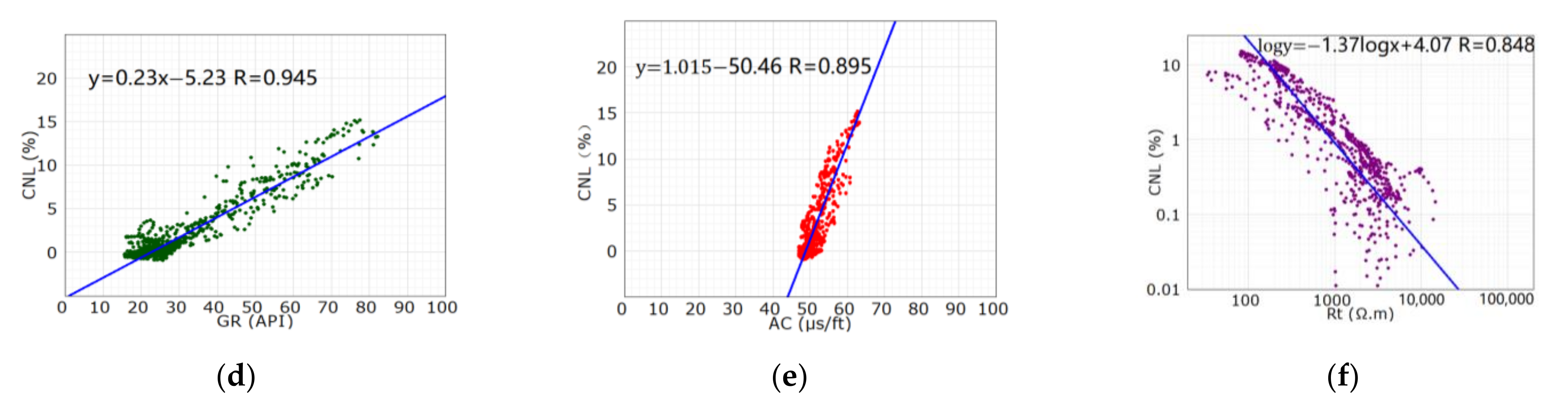
2. Basic Characteristics and Logging Response of the Feixianguan Formation Reservoir
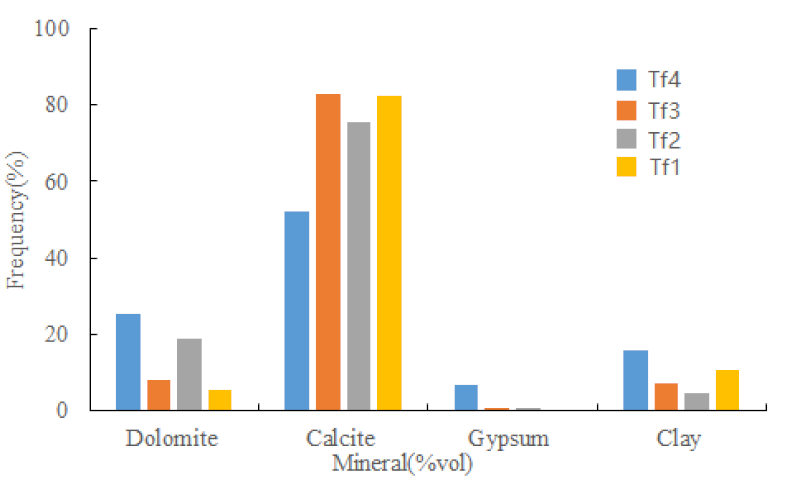
According to the petrochemical analysis, the mineralogical composition of the Feixianguan Formation in eastern Sichuan is mainly composed of clay, calcite, dolomite and gypsum. Namely: limestone, mudstone, dolomite and gypsum (by lithology) [2,3]. Brief introduction as follows: The limestone, mainly the oolitic limestone and the micrite limestone, is widely developed in this area. The fine-grained mudstone is mainly developed in the bottom of the Tf4 and Tf1. The gypsum is developed in the Tf4, and the rest of the formations appear in the form of the gypsum nodule occasionally. The oolitic dolomite and the oolitic limestone are the main reservoir rocks, and, among them, the oolitic dolomite is the best reservoir rock, but its development frequency is low; the oolitic limestone, in contrast, is high in development frequency, but, to be good reservoir, it has to be reformed by fracture reconstruction. The distribution of the various lithologies in the Feixianguan Formation is shown in Table 1.

Table 1.
Statistics of mineralogical composition of the Feixianguan Formation.
According to the core and the thin section calibration, the Feixianguan Formation reservoir is of the fracture-pore type, and the logging response shows low gamma, high acoustic wave, high neutron, low resistivity and positive difference characteristics. Figure 1 and Table 2 show the typical logging response characteristics of various lithologies.
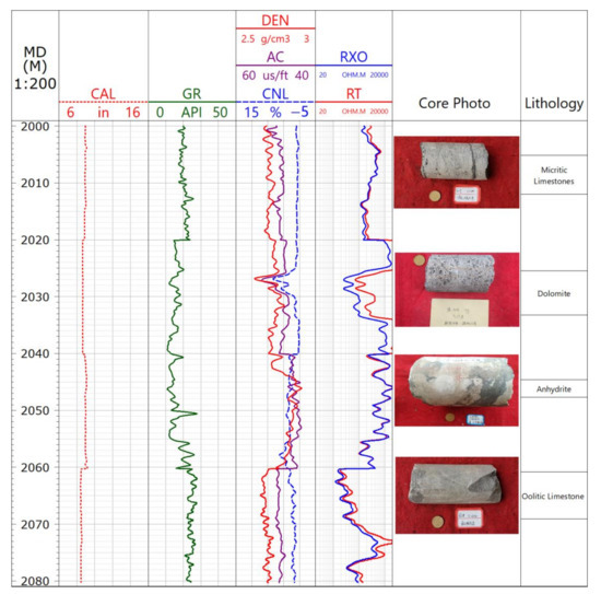
Figure 1.
Different lithology logging response characteristics in Feixianguan formation.
Table 2.
Different lithology logging response characteristics in Feixianguan formation.
3. Pseudo-Curve Reconstruction Method
According to the petrochemical analysis, the reservoir of the Feixianguan Formation is characterized by complex lithology and poor physical property. It can be seen from the logging response analysis that, normally, the complete conventional logging curve could indicate the lithologies and the physical properties of the reservoir better. In the light of the lithologic characteristics, the rock volume physical model can be simplified to five parts, namely, clay, gypsum, calcite, dolomite and porosity [1,4]. In order to solve five unknown quantities, we needed at least five curves to set up a system of simultaneous equations. However, out of a total of twelve wells in this area, only five old wells (X1–X5) had complete conventional logging curves; the remaining seven old wells (X6–X12) just had AC, GR and RT, RXO curves. Obviously, these old wells could only establish one underdetermined equation, including four equations and five unknown quantities, which could not meet the basic requirements of the quantitative solution of parameters of the complex carbonate reservoir. Therefore, it was unrealistic to expect the quantitative processing of complex lithology unless the pseudo-curve could be constructed and the underdetermined equation extended to the positive definite equation.
3.1. Selection of the Reconstruction Curves
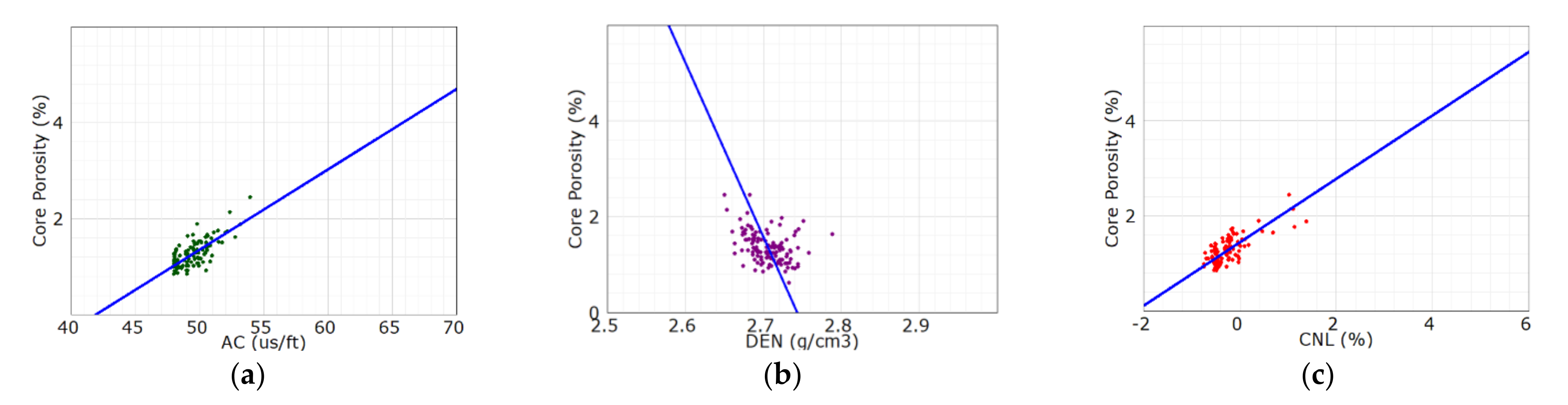
In order to reduce the error transfer and the uncertainty of the pseudo-curve, we had to make a choice between two logging curves, CNL and DEN, during the curve construction [5,6,7]. In this section, we will demonstrate the selection of the reconstruction curves. Firstly, by analyzing the crossplot of the core porosity of the coring section of well X1 and the 3-porosity curve (Figure 2), we found that the CNL curve was most significantly correlated with the core porosity, with the correlation coefficient of 0.71, less with the AC curve, and the least with the DEN curve, only 0.4. Obviously, the CNL curve could reflect the physical properties of reservoir better.
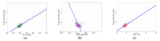
Figure 2.
Cross plot of the core porosity and the 3-porosity curve of well X1. (a) the core porosity versus the AC curve; (b) the core porosity versus the DEN curve and (c) the core porosity versus the CNL curve.
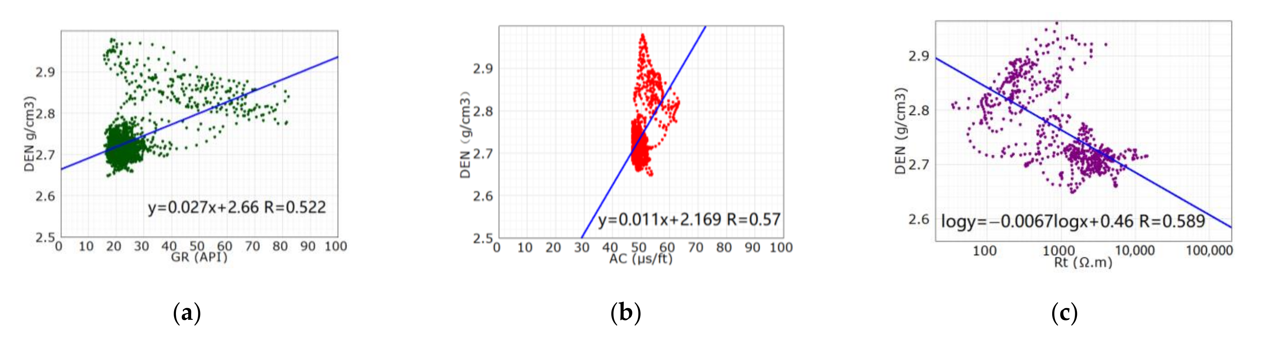
Secondly, we analyzed the relationship between the logging curves. It is known that the GR curve is sensitive to the clay, the AC, DEN and CNL curve can reflect the lithologies and physical properties of the reservoir simultaneously, and the RT curve can reflect the oil/gas-bearing properties [8,9]. We used the CNL curve and the DEN curve of well X1, respectively, to make a correlation analysis with other curves (Figure 3). It turned out that the correlation coefficients of the GR, AC and RT curve with the CNL curve were significantly higher than that with the DEN curve. The reason is that the high-density drilling fluid caused expansion of hole diameter and induced fracture in some sections of wells, which affected the AC curve and the DEN curve [10,11,12]. Therefore, it was more appropriate to reconstruct the CNL curve than the DEN curve.
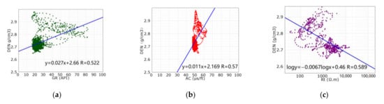
Figure 3.
Cross plot of the CNL curve, the DEN curve and other curves of the Feixianguan Formation of well X1. (a) the DEN curve versus the GR curve; (b) the DEN curve versus the AC curve; (c) the DEN curve versus the Rt curve; (d) the CNL curve versus the GR curve; (e) the CNL curve versus the AC curve… and (f) the CNL curve versus the Rt curve.
3.2. Selection of Construction Method
Regression is the essence of the old well curve reconstruction problem. At present, there are a lot of research and reports on the reconstruction methods for curves, including curve fitting, BP neural network, support vector machine, etc. [5,13,14,15]. These traditional reconstruction methods for curves basically have the same idea: Firstly, a certain number of the parameter eigenvalues are extracted, which form the training sample data set. Secondly, by using the mathematical algorithm, the corresponding curve prediction model is established [16]. The key of this technology is the convergence rate and the error analysis.
It is easy to find that, for the training data set, these traditional methods can obtain a good effect in self-judging ability but not in prediction effect [17]. Yet it is worth noting that, even if some methods can achieve good results, these have low accuracy of the curve construction to spoil the logging interpretation, which leads to multi-solution or even wrong interpretation [18,19]. Such a status quo is caused for the following reasons: Firstly, lack of the feature information leads to loss of details when we extract the parameter eigenvalue; secondly, lack of the training data leads to model over-fitting. Only a machine learning method with high generalization performance can break this dilemma [20]. Given that the logging data of unknown depth should be close within the nearby range when reconstructing curves, we chose the depth model BI-LSTM with a facility of drawing out the context sequence information to construct the pseudo-curve.
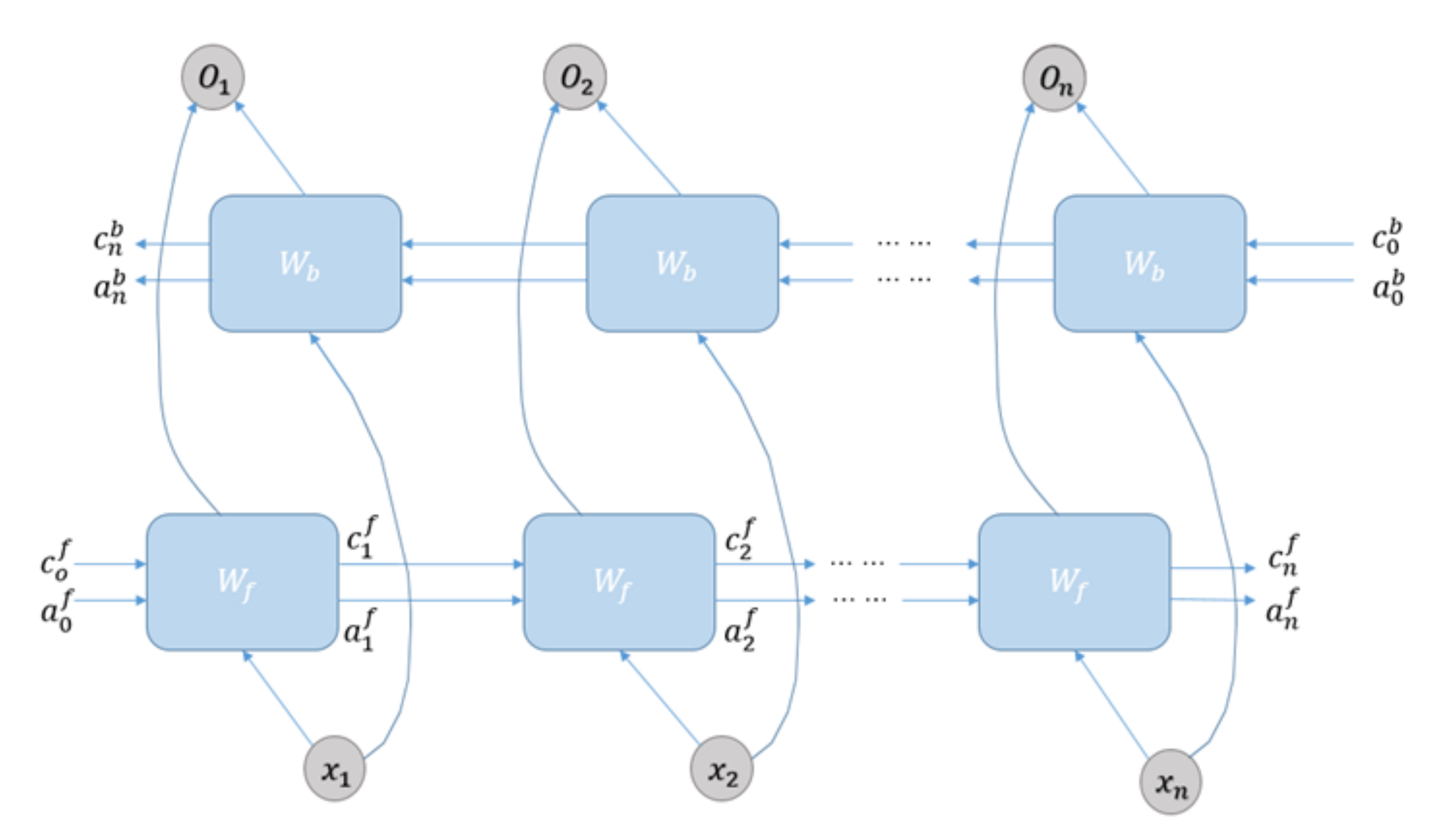
BI-LSTM is an extension of the recurrent neural network (RNN), which is a new method based on the common LSTM. By using BI-LSTM, we could divide one-way LSTM into two directions, namely the positive timing directions and the negative timing directions, and connect two networks to the same output by putting the forward information and the reverse information as the output of the current node at the same time [21,22]. BI-LSTM compensated for the limitations of the common neural network, solved the problem of “context semantic loss” caused by the lack of operation connection between each input layers, added the reverse operation based on the RNN and achieved the final results of the training data, namely the stacking of the forward RNN and the reverse RNN [23,24,25]. Beyond that, owing to the presence of LSTM, the imperfection of the RNN that cannot handle the long-term dependency information was also eliminated [26,27]. Figure 4 shows the schematic diagram of BI-LSTM network structure.
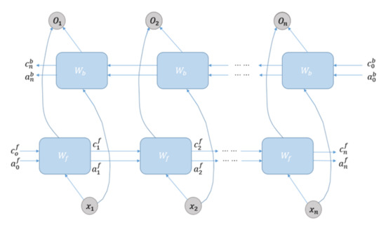
Figure 4.
BI-LSTM network structure diagram.
The algorithm can be expressed as:
where, is the input value of the BI-LSTM network at time t; is the output value of the BI-LSTM network at time t; is the value of the forward hidden layer at time t; is the value of the forward hidden layer at time t − 1; V is the weight of the output layer in the forward calculation; g is the corresponding activation function; U is the weight of the input layer; f is the corresponding activation function; W is the corresponding weight of the hidden layer; V′ is the weight of the output layer in reverse calculation; U′ is the weight of the output layer; W′ is the weight of the hidden layer; is the output of LSTM memory unit in reverse calculation at time t; and is the output of LSTM memory unit in reverse calculation at time t − 1. The output value of the BI-LSTM network at time t was obtained by the forward and reverse output.
3.3. Pseudo-Curve Reconstruction Experiment
Given the influence of the reservoir lithologies, the physical properties and the oil/gas-bearing properties on the logging curves, we used three logging curves, GR, AC and RT, as the input curves for CNL reconstruction. Taking the logging data of well X1 as the input sample and well X5 as the test sample, experiments were conducted by using multiple linear regression (MLR), BP neural network, support vector machine (SVM, and BI-LSTM [5,14,28]. According to the experiment results, the advantages of the reconstruction method for the curve can be discussed through three test parameters: the correlation coefficient (R), root mean square error (RMSE) and determination coefficient (R2). The closer R2 is to 1, the more accurate estimate is.
The concrete calculating methods are as follows.
SSres is the sum of squares of residuals, which can be calculated by Equation (4):
where, is real sample data, is sample average value and is estimated data.
SStot is the total sum of squares, which can be calculated by Equation (5):
R2 is the determination coefficient, which can be calculated by Equation (6):
The experimental results of well X1 and well X5 are shown in Table 3.
Table 3.
Statistical comparison table of different algorithms predict accuracy.
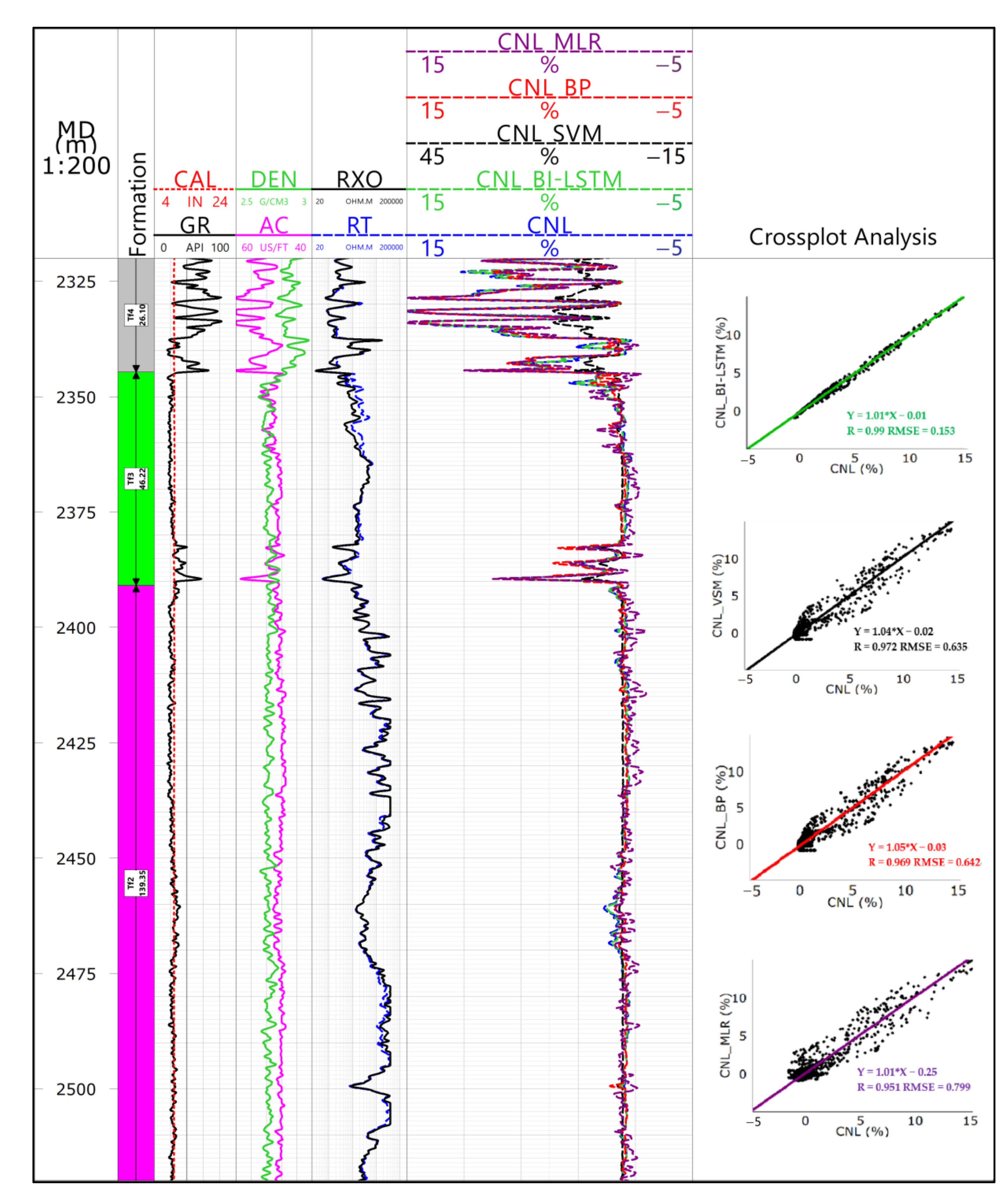
Figure 5 shows the effect of regression algorithms in well X1. Combined with Table 3, the self-judging curve was found to be consistent with the measured curve in the training set. Through contrastive analysis, we drew the conclusion: To the correlation coefficient (R), R of these regression algorithms were all greater than 0.95, showing good results; to the root mean square error (RMSE), BI-LSTM was the smallest, which was only 0.153, the multiple logistic regression (MLR) was the largest, which was 0.799, BP neural network and support vector machine lay halfway in between; to the determination coefficient (R2), SVM and BI-LSTM were the best, MLR was the worst. Briefly, all three parameters indicated that BI-LSTM was the optimal algorithm for the pseudo-curve construction.
Figure 5.
The back estimation sketch of well X1.
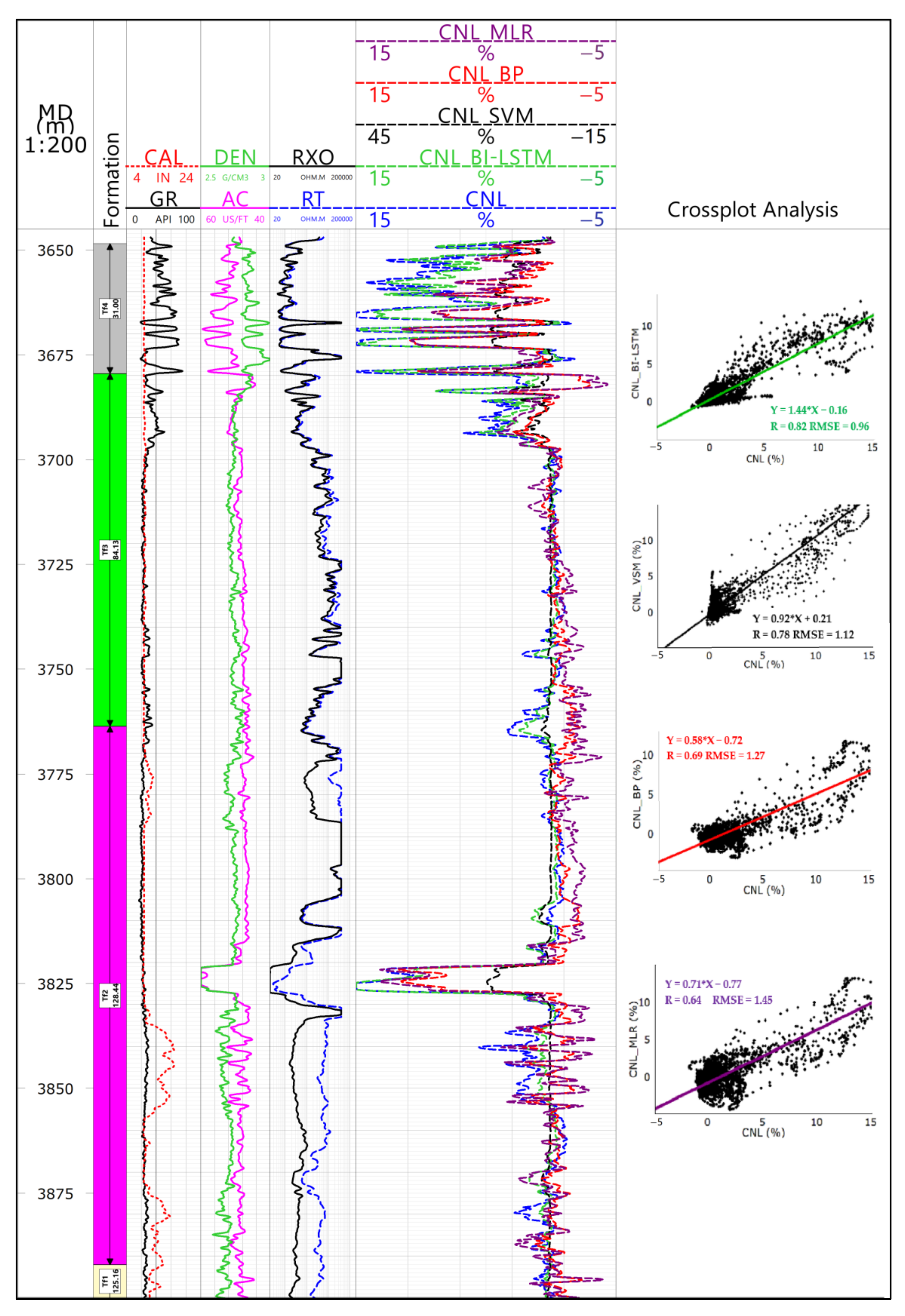
Figure 6 shows the prediction effect of different algorithms in well X5. The main contributions are as follows: For most well sections, the predicted curve was found to be consistent with the measured curve in trend and, for some well expansion sections, the predicted curve of the multiple regression and the BP algorithm was diametrically opposite to the measured curve. Three-parameter analysis showed that the prediction effect of these two algorithms was poor: R was less than 0.7, RMSE was greater than 1.2 and R2 was less than 0.6. In comparison, though the prediction effect of the support vector was rather ideal, BI-LSTM showed greater advantages. For BI-LSTM, R was significantly higher, RMSE was only 0.96 and R2 was up to 0.71. Through the BI-LSTM algorithm, we achieved a pseudo-neutron curve. For such a pseudo-neutron curve, the frequency band distribution range was narrower than the original curve, the high-gamma segment was smaller than the original curve and the low-gamma segment was larger than the original curve. After standardization, the pseudo-neutron curve was found to be consistent with the original curve in the low-gamma segment, but there was still a large error in the high-gamma segment. Significantly, the processing results did not interfere with the identification of the reservoirs and the calculation of the reservoir parameters, although large errors existed. The main reason for this is that the high-gamma segment was not the favorable reservoir.
Figure 6.
Forecast effect chart well X5.
Above all, the results show that the BI-LSTM network was the best method for pseudo-curve construction, which improved the prediction precision and the accuracy greatly. Through the BI-LSTM algorithm, the internal relationship of different logging curves was reconciled, the dependency relationship of the sample sequences in the logging domain was considered, the long-term dependence problem was solved and the perfect advantage of making full use of data information was reflected.
3.4. The Impact of Data Volume on Predicted Results
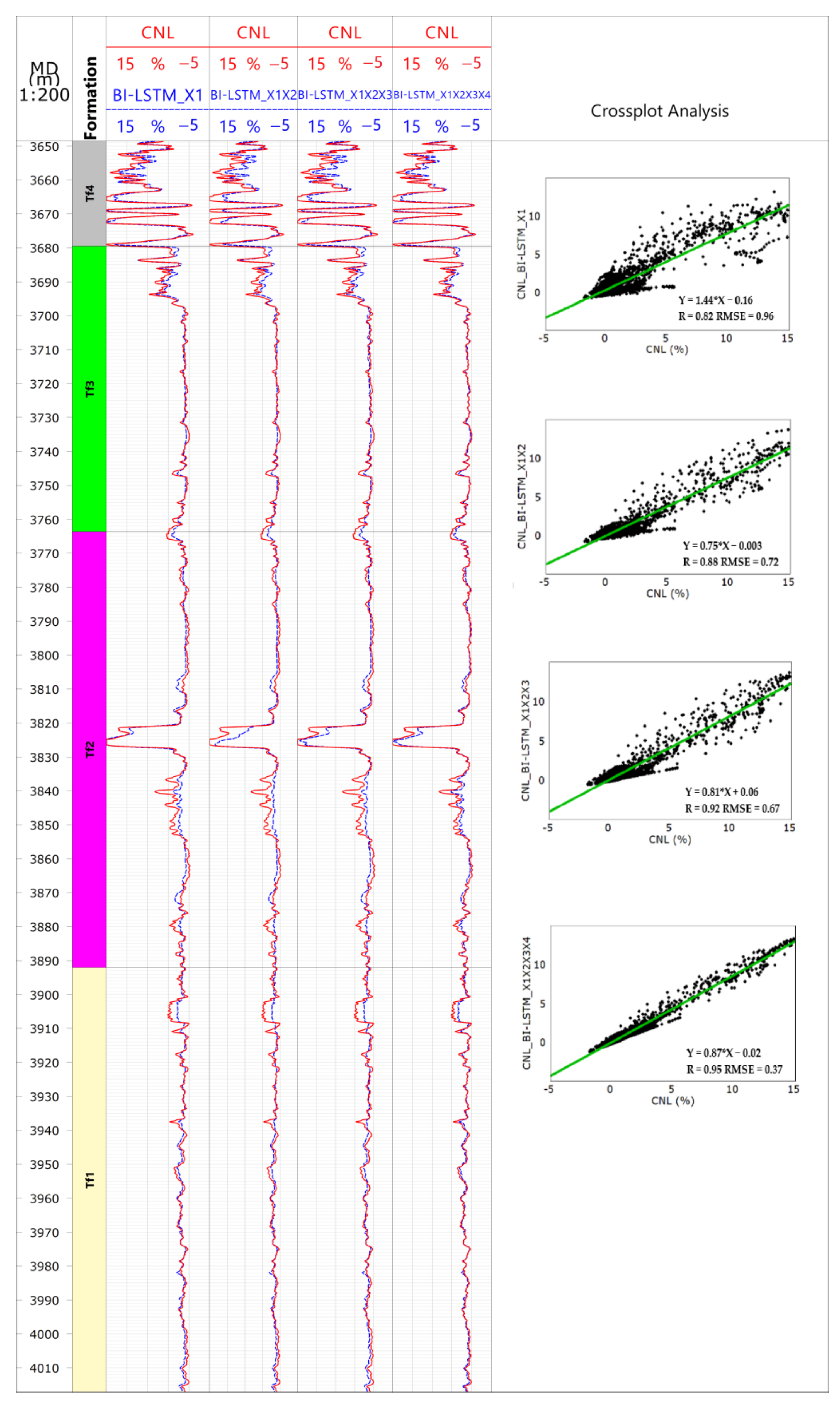
For the machine learning algorithm, in general, the more training samples we have, the more regularity information of the data set we achieve [4,29]. With the implementation of the training tasks and the accumulation of the experience, the model acquired a strong generalization ability. We took the data of well X1, X2, X3 and X4 as the training data in turn and took the data of well X5 as the effect test. This was done to discuss the influence of the data information on the prediction result of BI-LSTM.
It can be seen from the Figure 7 and Table 4 that, with the increase of the training data, there was a rising trend of the pseudo-curve prediction result in R and R2 but not for RMSE, suggesting that the prediction accuracy of BI-LSTM was improving. Yet it is worth noting that BI-LSTM was not affected by the data amount solely; when we took well X1 and well X2 as the training data set, R2 increased significantly from 0.71 to 0.76 but, with the addition of the training data of well X3 and well X4, the growth trend of R2 slowed down gradually.
Figure 7.
Prediction of BI-LSTM algorithm in well X5 data increment.
Table 4.
Experimental statistic BI-LSTM algorithm in data increment.
4. Application Effect Analysis
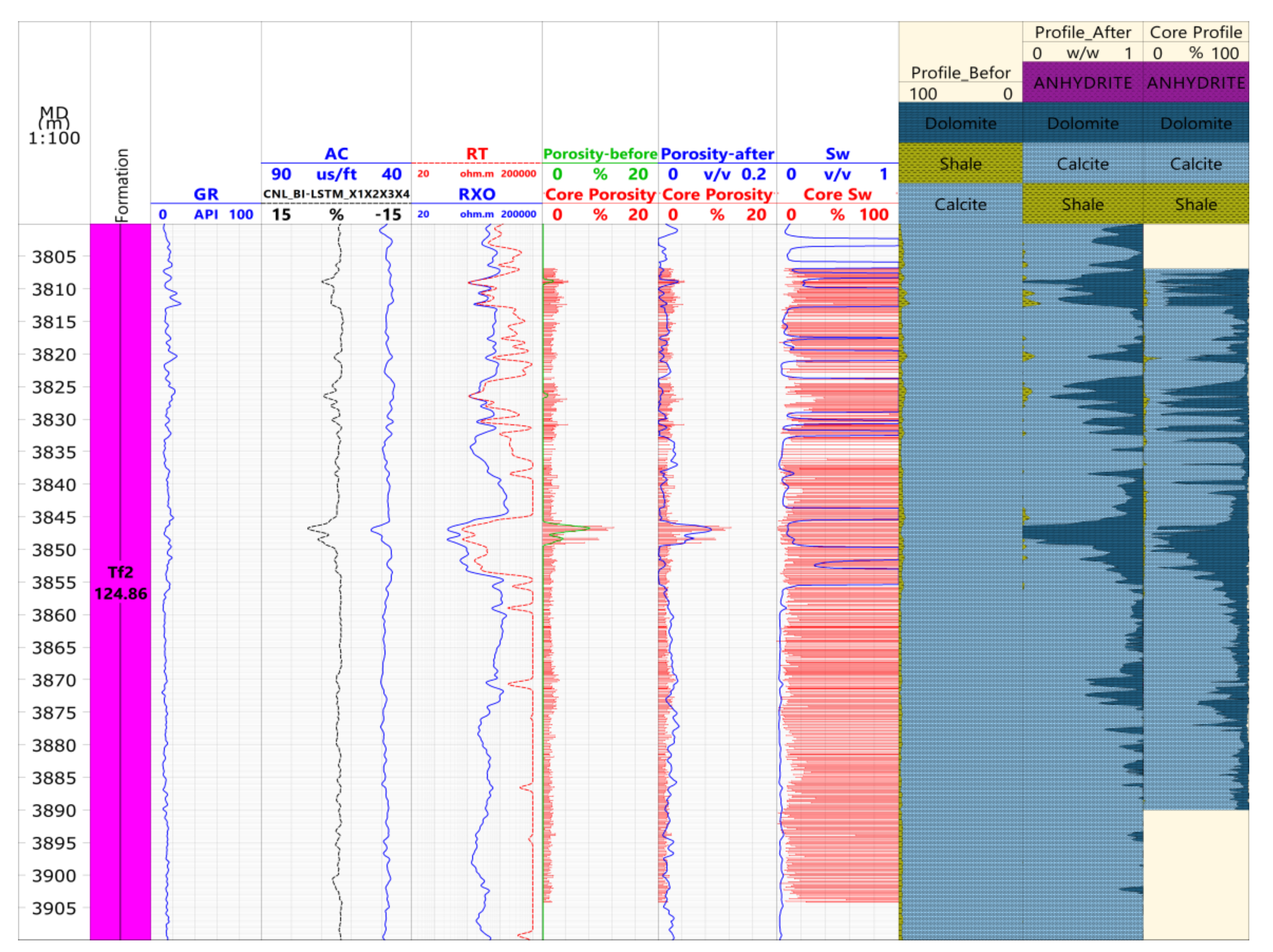
When using the optimized logging processing method for the data processing interpretation, note these points: the weight of the pseudo-neutron curve should be lower than 0.3, and the weight coefficient of the other measured curves should be set to 1. Figure 8 shows the comparison before and after the processing results of the pseudo-neutron curve construction in X6 old well. Before that, there were only four curves, GR, AC, RT and RXO. It means that the processing result can only be treated like a single limestone mineral, and the lithological, geophysical feature differs greatly from the core analysis data.

Figure 8.
Comparison of well X6 logging interpretation in lithology and physical properties.
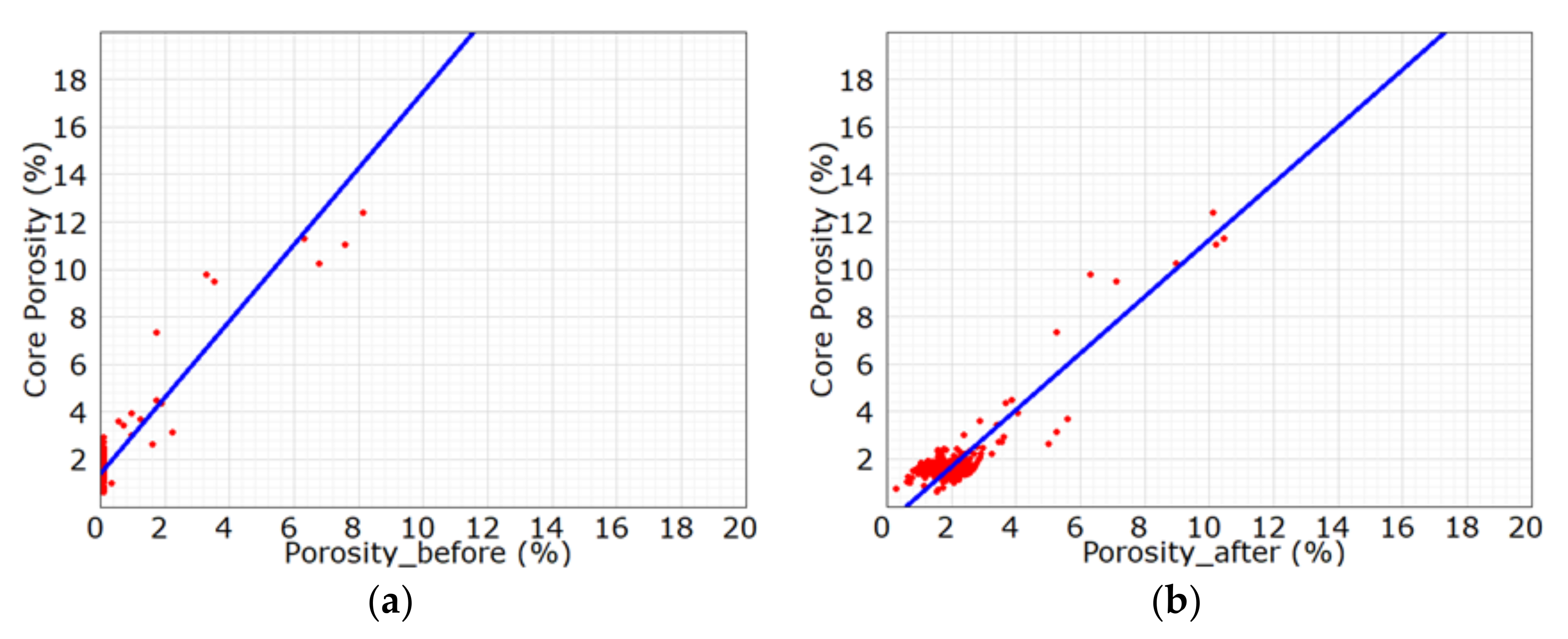
After that, the core porosity was found to be consistent with the logging porosity in trend, with a correlation coefficient of 0.896. For this kind of optimum processing result, the data points mostly distributed near the 45° line (Figure 9), the relative error was 14.7% and the absolute error was only 0.28. By comparison, the evaluation indexes were improved dramatically after curve construction (Table 5). The treated lithology profile was found to be consistent with the lithification analysis profile, basically, which demonstrates that the construction method of BI-LSTM curve is feasible.

Figure 9.
Cross plot of the core porosity and porosity of well X6. (a) the core porosity versus porosity before curve construction; (b) the core porosity versus log porosity after curve construction.
Table 5.
Index comparison table of before and after processing results of curve construction.
5. Conclusions
- (1)
- According to the correlation analysis of the core physical property and the 3-porosity curve in the Feixianguan Formation, the CNL curve is most significantly correlated with the core porosity, less with the AC curve and the least with the DEN curve. The results show that, compared with the DEN curve, in constructing the pseudo-curve, the CNL curve is a more rational choice.
- (2)
- Compared with the traditional method, BI-LSTM shows greater advantages. This method not only gives full consideration to the interdependence of the sample sequences in the logging depth domain, but also improves the construction precision and accuracy of the pseudo-curve by increasing the amount of data.
- (3)
- With the increase of the amount of training data, the prediction accuracy of the pseudo-curve constructed by BI-LSTM is gradually improved. Yet it is worth noting that BI-LSTM is not affected by the data amount solely.
- (4)
- By using BI-LSTM, the accuracy of the old well pseudo-curve is improved. However, it is suggested that the neutron curves should be standardized before being used for logging data processing and interpretation, and the weight coefficient should be reducing when using the curves.
Author Contributions
Conceptualization, Y.G. and C.C.; methodology, C.C.; software, S.J.; validation, J.Y.; formal analysis, L.Z.; investigation, Y.J.; resources, C.C.; data curation, Y.C.; writing original daft preparation, Y.G.; writing review and editing, C.C.; visualization, L.Z.; supervision, Y.J.; project administration, Y.C.; funding acquisition, Y.J. All authors have read and agreed to the published version of the manuscript.
Funding
This work is supported by the National Natural Science Foundation of China (no. 41430316); Funder: Jiang, Y.Q.
Institutional Review Board Statement
Not applicable.
Informed Consent Statement
Not applicable.
Data Availability Statement
The data sets used and/or analyzed during the current study are available from the corresponding author on reasonable request.
Conflicts of Interest
The authors declare no conflict of interests.
Abbreviations
| AC | acoustic |
| GR | natural gamma ray |
| Rt | true formation resistivity |
| Rxo | flushed zone formation resistivity |
| CNL | compensated neutron logging |
| DEN | density |
| Tf1~Tf4 | 1st~4st member of Feixianguan Formation |
References
- Liu, Y.T. Reservoir characteristics of Changxing-Feixianguan Formation in northeastern Sichuan area. Lithol. Reserv. 2019, 31, 78–86. [Google Scholar]
- Wei, G.; Yang, W.; Liu, M.; Xie, W.; Jin, H.; Wu, S.; Su, N.; Shen, J.; Hao, C. Distribution rules, main controlling factors and exploration direction of giant gas fields in the Sichuan Basin. Nat. Gas Ind. B 2020, 7, 1–12. [Google Scholar] [CrossRef]
- Jin, Y.J.; Zhang, Q.; Wang, M.M. Well logging curve reconstruction based on genetic neural network. Prog. Geophys. 2021, 36, 1082–1087. [Google Scholar]
- Liu, J.W.; Liu, Y.; Luo, X.L. Research and development on deep learning. Appl. Res. Comput. 2014, 31, 1921–1930. [Google Scholar]
- Zhao, J.L.; Li, G.; Ma, P.S.; Gong, Z.W.; Meng, L.F.; Li, G. The application of network technology to petroleum logging interpretation. Prog. Geophys. 2010, 25, 1744–1751. [Google Scholar]
- Qin, T.; Cai, J.Y.; Li, D.Y. Application of curve reconstruction technology in accurate reservoir prediction in Bohai Q oilfield. Comput. Tech. Geophys. Geochem. Explor. 2018, 40, 330–336. [Google Scholar]
- Salehi, M.M.; Rahmatii, M.; Karimnezhad, M.; Omidvar, P. Estimation of the non records logs from existing logs using artificial neural networks. Egypt. J. Pet. 2016, 26, 957–968. [Google Scholar] [CrossRef] [Green Version]
- Li, T.T.; Chen, J.R.; Guo, Y.; Pang, X.Y. A reservoir prediction application of density curve reconstruction in complex geological conditions. China Manganese Ind. 2019, 37, 19–23. [Google Scholar]
- Yu, J. Research on reservoir prediction technology based on curve reconstruction. Mod. Chem. Res. 2018, 11, 88–89. [Google Scholar]
- Duan, Y.X.; Li GT Sun, Q.F. Application of convolutional neural network in reservoir prediction. J. Commun. 2016, S1, 5–13. [Google Scholar]
- Yang, B.; Kuang, L.C.; Sun, Z.C.; Shi, J.C. Neural Network and Its Application in Petroleum Logging; Petroleum Industry Press: Beijing, China, 2005; pp. 94–98. [Google Scholar]
- Li, R.J.; Cui, Y.J.; Xiong, L. Evaluating conglomeratic sandstone reservoir in block C of Bohai oilfield by reconstructing neutron log. Well Logging Technol. 2019, 43, 427–433. [Google Scholar]
- An, P.; Cao, D.P.; Zhao, B.Y.; Yang, X.L.; Zhang, M. Reservoir physical parameters prediction based on LSTM recurrent neural network. Prog. Geophys. 2019, 34, 1849–1858. (In Chinese) [Google Scholar]
- Yang, Z.L.; Zhou, L.; Peng, W.L.; Zheng, J.Y. Application of BP neural network technology in sonic log data rebuilding. J. Southwest Pet. Univ. (Sci. Technol. Ed.) 2008, 30, 63–66. (In Chinese) [Google Scholar]
- Zhu, G.J. Application of acoustic curve reconstruction in reservoir prediction. Comput. Tech. Geophys. Geochem. Explor. 2017, 39, 383–387. [Google Scholar]
- Zhou, X.; Cao, J.X.; Wang, X.J.; Wang, J.; Liao, W.P. Acoustic log reconstruction based on bidirectional gated recurrent unit neural network. Prog. Geophys. 2021, 1–11. Available online: http://kns.cnki.net/kcms/detail/11.2982.P.20210209.1209.009.html (accessed on 29 December 2021).
- Han, B.H.; Wang, F.; Liu, Q.R.; Zhang, C.A. Review of research progress on evaluation of logging reservoir classification methods. Prog. Geophys. 2021, 36, 1966–1974. [Google Scholar]
- Hou, X.L.; Hu, Y.; Li, Y.Q.; Xu, X.H. Rational structure of multi-layer artificial neural network. J. Northeast. Univ. (Sci. Technol. Ed.) 2003, 24, 35–38. [Google Scholar]
- Zheng, Y.Z.; Ye, Z.H.; Liu, X.A.; Zhao, L. Research on prediction method of reservoir physical properties based on deep learning. Electron. World 2018, 10, 23–26. [Google Scholar]
- Wei, L.H.; Guo, J.Y.; Yang, Z.L.; Huang, Y.F. Analysis on key techniques of log constrained lithological inversion. Nat. Gas Geosicience 2006, 17, 731–735. [Google Scholar]
- Cheng, X.; Cheng, Y.X.; Cheng, J.H.; Sun, Q.L. Geophysical logging system based on machine learning and big data technology. J. Xi’an Univ. Pet. (Nat. Sci. Ed.) 2019, 34, 108–116. [Google Scholar]
- Zhou, X.Q.; Zhang, Z.S.; Zhu, L.Q.; Zhang, C.M. A new method for high-precision fluid identification in bidirectional long short-term memory network. J. China Univ. Pet. (Ed. Nat. Sci.) 2021, 45, 69–76. [Google Scholar]
- Alizadeh, B.; Najjari, S.; Kadkhodaie-Ilkhchi, A. Artificial neural network modeling and cluster analysis for organic facies and burial history estimation using well log data: A case study of the South Pars Gas Field, Persian Gulf, Iran. Comput. Geosci. 2012, 45, 261–269. [Google Scholar] [CrossRef]
- Bengio, Y.; Simard, P.; Frasconi, P. Learning long-term dependencies with gradient descent is difficult. IEEE Trans. Neural Netw. 1994, 5, 157–166. [Google Scholar] [CrossRef]
- Hochreiter, S.; Schmidhuber, J. Long short-term memory. Neural Comput. 1997, 9, 1735–1780. [Google Scholar] [CrossRef] [PubMed]
- Hornik, K. Approximation capabilities of multilayer feedforward networks. Neural Netw. 1991, 4, 251–257. [Google Scholar] [CrossRef]
- Zhang, B.L.; Luo, D.T.; Hu, P.; Fan, J.; Jin, C. A well log curve generation method based on deep neural network. Electron. Meas. Technol. 2020, 43, 107–111. [Google Scholar]
- Li, C.B.; Fan, J.F.; Song, X.L. A study on application of deep learning in geology. Jiangsu Geol. 2018, 42, 115–121. [Google Scholar]
- Zhang, D.X.; Chen, Y.T.; Meng, J. Synthetic well logs generation via recurrent neural networks. Pet. Explor. Dev. 2018, 45, 598–607. [Google Scholar] [CrossRef]

Publisher’s Note: MDPI stays neutral with regard to jurisdictional claims in published maps and institutional affiliations. |
© 2022 by the authors. Licensee MDPI, Basel, Switzerland. This article is an open access article distributed under the terms and conditions of the Creative Commons Attribution (CC BY) license (https://creativecommons.org/licenses/by/4.0/).