Abstract
Reaction networks can be simplified by eliminating linear intermediate species in partial steady states. In this paper, we study the question whether this rewrite procedure is confluent, so that for any given reaction network with kinetic constraints, a unique normal form will be obtained independently of the elimination order. We first show that confluence fails for the elimination of intermediates even without kinetics, if “dependent reactions” introduced by the simplification are not removed. This leads us to revising the simplification algorithm into a variant of the double description method for computing elementary modes, so that it keeps track of kinetic information. Folklore results on elementary modes imply the confluence of the revised simplification algorithm with respect to the network structure, i.e., the structure of fully simplified networks is unique. We show, however, that the kinetic rates assigned to the reactions may not be unique, and provide a biological example where two different simplified networks can be obtained. Finally, we give a criterion on the structure of the initial network that is sufficient to guarantee the confluence of both the structure and the kinetic rates.
1. Introduction
Chemical reaction networks are widely used in systems biology for modeling the dynamics of biochemical molecular systems [1,2,3,4]. A chemical reaction network has a graph structure that can be identified with an (unmarked) Petri net [5]. Beside of this, it assigns to each of its reactions a kinetic rate that models the reaction’s speed. Chemical reaction networks can either be given a deterministic semantics in terms of ordinary differential equations (Odes), which describes the evolution of the average concentrations of the species of the network over time, or a stochastic semantics in terms of continuous time Markov chains, which defines the evolution of molecule distributions of the different species over time. In this paper, we focus on the deterministic semantics.
Reaction networks modeling molecular biological systems—see, e.g., the examples in the BioModels database [6]—may become very large if modeling sufficient details. Therefore, biologists like to abstract whole subnetworks into single black-box reactions, usually in an adhoc manner that ignores kinetic information [7,8]. The absence or loss of kinetic information, however, limits the applicability of formal analysis techniques. Therefore, much effort has been spent on simplification methods for reaction networks that preserve the kinetic information (see [9] for an overview).
The classical example for a structural simplification method is Michaelis-Menten’s reduction of enzymatic networks with mass-action kinetics [10]. It removes the intermediate species—the complex C and enzyme E—under the assumption that their concentrations and are quasi steady, i.e., approximately constant for all time points t after a short initial phase. Segel [11] shows how to infer Michaelis-Menten’s simplification from the assumptions that is constant and that the conservation law holds. This is equivalent to our exact steadiness assumption for both and .
The Odes for C inferred from this network jointly with exact steady state assumptions for C and E entail that the concentration of substrate S must be constant too, even if the network is used in a bigger context where the intermediate C is neither produced nor consumed. In the literature, this consequence is usually mentioned but ignored when considering the production rate of product P as a function of the concentration of S for the enzymatic network in isolation (see e.g., [12]). This oversimplification can be avoided when studying the enzymatic network in the context of a larger network. For instance, the steady state assumptions for C, E, and thus S can be satisfied in the context of the reaction network with the reaction which produces S with constant speed , and the reaction which degrades P with mass-action kinetics with rate constant . In this context, the concentration of P will saturate quickly under exact steady state assumptions for C, E, and thus S, as illustrated in Figure 1, while in other contexts it may grow without bound or even oscillate. The Michaelis-Menten simplification of the enzymatic network indeed preserves the dynamics of a network in any context which does not produce nor consume the intermediates E and C, under the assumption that E and C are exactly in steady state with respect to the network in the context.
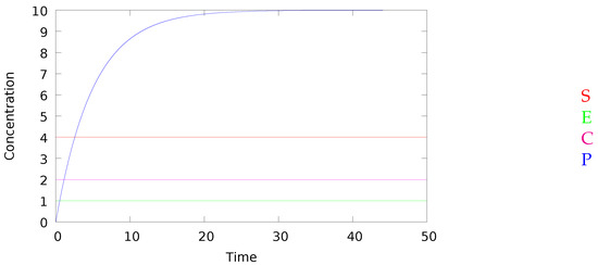
Figure 1.
Evolution of the concentration of , , and in enzymatic network with mass-action kinetics with the parameters , the initial concentrations , , , , and in the context of the network with a reaction which produces S with constant speed , and a reaction which degrades P with parameter .
Whether exact steady state assumptions are realistic is an interesting question since the concentrations may be at most close to steady in practice. In the literature it has been argued that the Michaelis-Menten simplification yields a good approximation under appropriate conditions [11,13,14], which typically depend on the context. Whether such properties can be extended to more general simplification methods as developed in the present article is an interesting question but out of the scope of the paper.
Alternatively, much work was spent on simplifying the Odes inferred from a given reaction network [15,16], rather than the reaction network by itself. Indeed, any structural simplification method on the network level, that preserves the kinetic information with respect to the deterministic semantics, must induce a reduction method on the Ode level. The opposite must not be true, since some Odes may not be derivable from any reaction network or may be inferred from many different ones [17]. Furthermore, it is not clear what it could mean for an Ode simplification method to be contextual. Therefore, Ode simplification alone cannot be understood as a simplification of biological systems.
A general structural simplification algorithm for reaction networks with deterministic semantics was first presented by Radulescu et al. They proposed yet another method [18] for simplifying reaction networks with kinetic expressions in partial steady states. Their method assumes the same linearity restriction considered in this paper, preserves exactly the deterministic semantics, but uses different algorithmic techniques. Their simplification algorithm is based on a graph of intermediate species. It computes cycles for simplifying the network structure rather than on elementary modes, and spanning trees for simplifying the kinetic expressions. A set of intermediate species is eliminated in one step, leading to a unique result, that is included in the results found with the algorithm of the present paper. We have not understood yet what distinguishes this result from the others obtained with our algorithm; a clarification of this point might shed light on the relationship between the two methods. In the same paper, the authors also observe that applying the method iteratively to intermediates one by one leads to different results even with different structure. The reason is that dependency elimination is lost in this manner.
A purely structural simplification algorithm method for reaction networks without kinetic rates was proposed in [19]. The method allows to remove some intermediate species by combining the reaction producing and consuming them. For instance, one can simplify the network with the following two reactions on the left into the single reaction on the right, by removing the intermediate species B:
Since no partial steady state assumptions can be imposed in a kinetics free framework, the intermediate elimination rules need some further restrictions. Given these, the simplification steps were shown correct with respect to the attractor semantics. contextual equivalence relation was obtained by instantiating the general framework for observational program semantics from [20]. Rather than being based on termination as observable for concurrent programs, it relies on the asymptotic behaviours of the networks represented by the terminal connected components, which are often called attractors.
Outline
We first recall some basic notions on confluence, multisets, and commutative semigroups in Section 2. In Section 3 we recall the basics on reaction networks without kinetics and elementary flux modes. In Section 4, we present the rewrite rules for intermediate elimination, illustrate the failure of confluence, and propose a rewrite rule for eliminating dependent reactions, which however turns out to be non-confluent on its own. In Section 5 we present the refined algorithm in the case without kinetics based on the notion of flux networks for representing reaction networks, and prove its confluence by reduction to a folklore result on elementary flux modes. In Section 6, we introduce reaction networks with kinetic expressions, and extend them with kinetic constraints. In Section 7, we lift the revised algorithm to constrained flux networks with kinetics. In Section 8 we present a linearity restriction, that is preserved by reductions, and thus structurally confluent. In Section 9, we present a counter example that shows that full confluence is still not achieved, and present a further syntactic restriction based on elementary modes avoiding this problem. Section 10 provides a biological example of non-confluence with kinetics. Section 11 studies the relation between the simplification and the underlying Odes simplification. Finally, we conclude in Section 12.
2. Preliminaries
We recall basic notions on confluence of binary relations, on multisets, and more general commutative semigroups. We will denote the set of all natural numbers including 0 by and the set of integers by .
2.1. Confluence Notions
We recall the main confluence notions and their relationships from the literature.
Let be a set with an equivalence relation and a binary relation. In most cases, ∼ will be chosen as the equality relation of the set S, which is . We define and for all . The relation is called the reflexive transitive closure of →.
Definition 1.
We say that a binary relation → on is confluent if and locally confluent if . We say that two binary relations ⇒ and → on S commute if .
The confluence notions are illustrated by the diagrams in Figure 2. Clearly, a confluence of relation → is confluent if its reflexive transitive closure commutes with itself. It is also obvious that local confluence implies confluence, and well known that the converse does not hold. In this paper, we will always use binary relations that are terminating, i.e., for any there exists a such that , i.e., the length k of sequences of reduction steps starting with s is bounded. It is well known that locally confluent and terminating relations are confluent (Newman’s lemma).
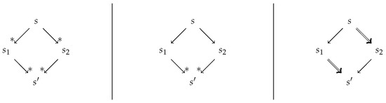
Figure 2.
Confluence, local confluence, and commutation.
Lemma 1.
If a binary relation → on is confluent and commutes with ∼, then the binary relation on is confluent.
Definition 2.
Let and be two sets each endowed with two binary relations. A function is called a simulation from to if for any , if then , and if then .
The conditions that have to be satisfied by simulations are illustrated by the diagrams in Figure 3.
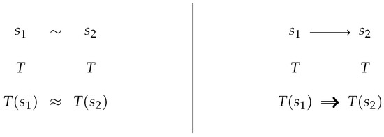
Figure 3.
Simulation diagrams.
2.2. Multisets
Let R be a finite set. A multiset M with elements in R is a function . For any we call the number of occurrences of r in M. We say that r is a member of multiset M and write if . We denote by the set of all multisets (over R), and will simply write if the set R is clear from the context.
Given numbers and a subset with k different elements, we denote by the multiset that for any contains occurrences of and occurrences of all other elements in R.
The sum of two multisets is the multiset M that satisfies for all . The empty multiset is the function that maps all elements of R to 0. The algebra of multisets over a given set R is a commutative semigroup with a neutral element.
It should be noticed that our notation may give rise to some ambiguities, since we will also write + for the addition of natural numbers instead of . This may be problematics if . In this case, the notation introduced below we will permit us to write for sums of multisets and for sums of natural numbers.
2.3. Commutative Semigroups
Let and be two semigroups with neutral element. Beside of the algebras of multisets (depending on the choice of R) we are interested in the algebra of vectors of naturals for any .
A homomorphism between two semigroups is a function such that for all and . A homomorphism on multisets is determined by the values of h on singleton multisets in via the equation:
Given a homomorphism , we define the interpretation for all multisets . Clearly, the interpretation depends on the homomorphism h, even though only its co-domain appears in our notation. This works smoothly since there will never be any ambiguity about the homomophism that is chosen. If , then we use the homomorphism with for all elements . In this case, any multiset with elements in is evaluated to a single element and thus by the above equation:
If then we use the identity homomorphism with for all . In this case we have that is the multiset itself.
We will also use this notation in order to distinguish the operator + of multisets in from the operator + of natural numbers in which we overloaded (as stated earlier). For instance, if , then is a multiset of natural numbers while is a natural number. Note also that different multisets may have the same interpretation. For instance if and , then where we use as homomorphism while where we use as homomorphism.
For any subset of a semigroup, we can define the (positive integer convex) cone of G, as the set of all positive integer linear combinations of elements of G:
Here we use as homomorphism.
3. Reaction Networks without Kinetics
Let be a finite set of species that is totally ordered. A (chemical) solution with species in is a multiset of species . A (chemical) reaction with species in is a function , which assigns to each species A the stoichiometry of A in r. A chemical reaction r consumes the chemical solution and produces the chemical solution . Clearly for all species A, while and are disjoint multisets in chemical reactions r (since their definition is based on stoichiometries).
We will freely identify a reaction r with the pair of chemical solutions consumed and produced by r. We will denote such pairs as . For instance, is the chemical reaction r with , , and . Note also that we do not consider as a chemical reaction, since the species A belongs to the chemical solutions on both sides. When removing on both sides, we obtain a chemical reaction . The rewrite relation of a chemical reaction r contains all pairs of chemical solutions such that for all species A.
Definition 3.
A reaction network (without kinetics) over is a finite set of chemical reactions over , with a total order.
To any reaction network N with total order < we assign a unique vector of reactions such that and . Conversely, for any tuple of distinct reactions , we write for the reaction network with the total order .
Any reaction network can be represented by a bipartite graph as for a a Petri net, with a node for each species and a node of a different type for each reaction. We will draw species nodes with ovals and reaction nodes with squares. An arrow labeled by k from the node of a species A to the node of a reaction r means that A is consumed k times by r, i.e., . Conversely, an arrow with label k from the node of a reaction r to the node of a species A means that A is produced k times by r, i.e., . We will freely omit the labels .
Example 1.
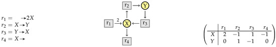
Consider the reaction network presented in Figure 4. It has species and reactions in that order. Reaction produces two molecules of species X out of nothing, reaction transforms an X into a molecule Y, while transforms a molecule Y back into a molecule X. Reaction degrades a molecule X.
Figure 4.
A reaction network and the associated graph and stoichiometry matrix.
The set of chemical reactions defines an algebra where is the empty reaction →, and is the addition of integer valued functions on . Note that for any two disjoint chemical solutions s and . By interpretation in this algebra (that is using the identity homomorphism), we can evaluate each multiset of chemical reactions M as a chemical reaction itself, as shown in Section 2.2.
Definition 4.
An invariant of a reaction network N without kinetics is a multiset M of reactions of N such that . We denote the set of all invariants of N by .
The reaction network in Figure 4 has the set of invariants where and . We next relate the notion of invariants of a reaction network to the kernel of its stoichiometry matrix.
3.1. Stoichiometry Matrices
The stoichiometry information of a reaction network is usually collected in its stoichiometry matrix. For this we consider a set of species and a reaction network , such that both sets are totally ordered by the indices of their elements.
The stoichiometry matrix S of N is the matrix of integers, such that the entry of S at row i and column j is equal to for all and . Note that reaction contributes in the column, while species contributes the j’s row of S. For instance, the stoichiometry matrix of the reaction network in Figure 4 is given on the right.
It can now be noticed that, for any vector of natural numbers, the multiset is an invariant of reaction network N if and only if its stoichiometry matrix satisfies , i.e., if v belongs to the kernel of the stoichiometry matrix. Therefore, we define the (positive integer) kernel of a matrix S by:
3.2. Elementary Modes
The support of a vector is the subset of indices i such that is non-null, i.e., .
Definition 5.
An elementary mode of an matrix S over is a vector such that:
- v is on an extreme ray: there exists no such that , and
- v is factorised: there exists no such that for some natural number .
The condition means that an elementary mode must be a (positive integer) steady state of S. Geometrically, the set of all positive integer steady states forms a pointed cone, that is generated by convex combinations of its extreme rays. The first condition states that any elementary flux mode v must belong to some extreme ray of the cone. The second condition requires that an elementary mode is maximally factorised, i.e., it is the vector on the extreme ray with the smallest norm.
Theorem 1
(Folklore [21]). Let S be an matrix of integers. Then the set E of all elementary modes of S has finite cardinality and satisfies .
The intuition is is a cone with a finite number of extreme rays, so that these extreme ray generated the cone. The set of elementary modes E contains exactly one point on each of the extreme rays of . Therefore, , i.e., the set of elementary modes is a finite generator of .
Let us point out two differences between the definition of elementary mode considered here and in [21]. First, we added condition 2. Without this condition, any multiple of an elementary mode would be an elementary mode, so that there would be infinitely many. The double-description method as recalled there, however, computes the set of elementary modes in the above sense, so this difference is minor. Second, note that [21] considers a slightly more general problem, where some of the coordinates of v may be negative. This corresponds to the addition of reversible reactions that we do not consider in the present paper.
3.3. Elementary Flux Modes
We next lift the concept of elementary modes from matrices to reaction networks, via the stoichiometry matrix. Given a vector of reactions and a vector of natural numbers we define the multiset of reactions and the corresponding reaction as follows:
Definition 6.
An elementary flux mode of a reaction network is a multiset of reactions such that the vector v is an elementary mode of the stoichiometry matrix of N.
The kernel condition of elementary modes v yields that any elementary flux mode satisfies , i.e., the reaction defined by the elementary flux mode must be empty. For instance, reconsider the reaction network in Example 1 with species and reactions in that order. Its stoichiometry matrix has two elementary modes: the vectors and . The corresponding elementary flux modes are the multisets of reactions and illustrated in Figure 5 by the arrows coloured in apricot and aquamarine respectively. First consider the multiset : the first reaction produces which are then degraded by . So the reaction is indeed empty. Consider now the multiset of reactions : its first reaction transforms X to Y and its second reaction does the inverse. Thus, is the empty reaction too. The intuition is that applying to a chemical solution at the same time all reactions of an elementary flux mode with their multiplicities does not have any effect.
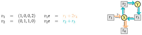
Figure 5.
The elementary modes of the reaction network in Figure 4.
It should be noticed that the vector is also a solution of the steady state equation , and thus the multiset of reactions is also an invariant of the example network. It is the multiset sum of two elementary flux modes which is also equal to .
4. Simplifying Reaction Networks without Kinetics
We study the question whether the step-by-step intermediate elimination relation proposed in [22] is confluent in the case of reaction networks without kinetics. We present a counter example against the confluence and illustrate the reason for this problem.
4.1. Intermediate Elimination
Let be a finite set of species that we will call intermediate species or intermediates for short. The simplification procedure will remove all intermediates from a given reaction network, step-by-step and in arbitrary order.
Our objective is to remove an intermediate from a network N by merging any pair of reactions of N, a reaction r that produces X and another reaction that consumes it. This is done by the (Inter) rule in Figure 6, and is based on the merge operation which returns a linear combination of and thus of the reactions in the initial network:
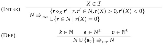
Figure 6.
Simplification of reaction networks without kinetics with respect to a set of intermediate species.
Since produces molecules X while consumes molecules X, we have () (X) = 0. Therefore, X is not present in the solutions consumed and produced by reaction .
In Example 2 below, we will denote vectors of natural numbers by , while freely omitting components with and simplifying component to j. For instance if , we can write instead of .
Example 2.
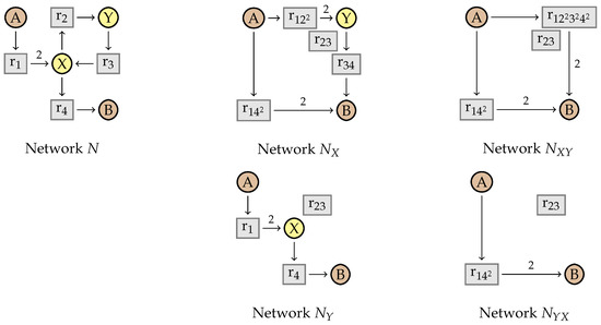
We consider the network in Figure 7 with species and reaction vector . We consider the elimination of the intermediates in in both possible orders. On the top, we first eliminate the intermediate species X from , obtaining network . We have to combine reaction producing 2 X molecules with reaction which consumes 1 X molecule. We obtain the reaction that transforms one A molecule into 2 Y molecules. We proceed in the same way with the other 3 pairs of reactions that produce and consume X. Then, we can remove the intermediate species Y from network and obtain the network in the top right. Note that we keep empty reactions such as . At the bottom, we show network , obtained by eliminating the intermediate species Y first. The only reaction producing Y in N is and the only reaction consuming Y is . Merging them produces reaction . When eliminating intermediate X from , we obtain network on the bottom right.
Figure 7.
Elimination of intermediates X and Y in reaction network in both possible orders, leading to two different final results and .
It turns out that and differ in that the former contains the reaction in addition to the reactions and shared by both networks.
4.2. Eliminating Dependent Reactions
Example 2 shows that intermediate elimination with the (Inter) rule alone is not confluent, given that it may produce two different networks that cannot be simplified any further, and , depending on whether we first eliminate the intermediate X or the intermediate Y. The reaction network contains an additional reaction, which is a linear combination of two other reactions:
In order to solve this non-confluence problem, we propose the new simplification rule (Dep) in Figure 6. It eliminates a reaction that is a positive linear combination of other reactions of the network, i.e., some reaction where and for some .
Unfortunately, the simplification relation with rules (Inter) and (Dep) is still not confluent. The problem is that even applying rule (Dep) alone fails to be confluent as shown by the following counter example.
Example 3.
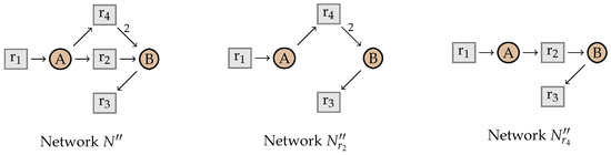
Consider the network in Figure 8 in the absence of intermediates, i.e., where . There are two ways of applying rule (Dep) to this network, since and . We can thus either eliminate leading to or leading to . The two results are different even though they contain no more dependencies.
Figure 8.
Dependency elimination is not confluent.
This example shows that general dependency elimination cannot be done in a confluent manner. On the other hand, what we need in order to solve the confluence problem for intermediate elimination as illustrated in Figure 7, is a little more restricted: it is sufficient to remove those dependent reactions that were introduced by intermediate elimination. Such dependencies can be identified from the vectors of natural numbers that we used to name the reactions. In the example, we have , so the dependency of this reaction follows from the dependency of the vectors .
5. Simplifying Flux Networks
We next introduce vector representations of reaction networks without kinetics, called flux networks, and show that the simplification of such representations can indeed be done in a confluent manner.
For the reminder of this section, we fix an n-tuple of distinct reactions and a subset of species .
5.1. Vector Representations of Reaction Networks
The objective is to simplify the initial reaction network by removing the intermediates from . The iterative elimination of intermediate species generates a sequence of networks with reactions in . The idea is now to use the vectors as representations of reactions . These vectors will tell us about the provenance of the reaction obtained when simplifying the network .
The mapping of vectors to reactions is a homomorphism between commutative semigroups, whose image is . It should be noticed, however, that it is not an isomorphism since any element of will be mapped to , where S is the stoichiometry matrix of . Therefore, it makes a difference whether we will work with vectors in representing a reaction or with the reactions itself. Intuitively, the difference is that we know where the reaction does come from.
Definition 7.
An n-ary flux network V is a finite subset of vectors in that is totally ordered.
Any n-ary flux network V defines a reaction network , that we call the reaction network represented by V. The total order of the reactions in network is the one induced by the total order of V.
5.2. Simplification Rules
Let be a finite set of species that we call intermediates. In Figure 9, we rewrite the simplification rules (F-Inter) and (F-Dep) so that they apply to flux networks. For this we have to lift the merge operation from reactions to vectors that represent them. For any we define:
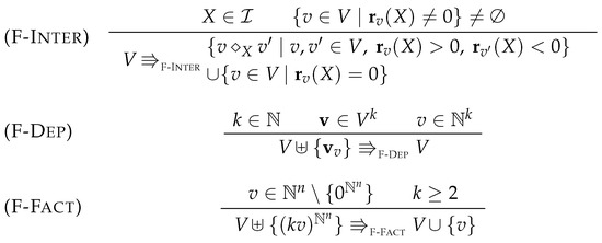
Figure 9.
Simplifying flux networks for an initial n-tuple of reactions and a set of intermediate species .
In the rule for the dependency elimination, we now use a notation for linear combinations of vectors in . Given a vector of vectors in and a vector of natural numbers we define:
The counter example for the non-confluence of dependency elimination can no more be applied in this way, since rule (F-Dep) is not based on the dependency of the reactions as with (Dep) but on the dependencies of the vectors that define the reactions.
5.3. Factorization
The simplification relation with axioms (F-Inter) and (F-Dep) is still not confluent, as shown in Example 4.
Example 4.
We consider the vector of initial reactions of the network in Figure 10. Let be the set of intermediate species. Note that where is the flux network to which we apply the simplification algorithm. If we remove the species X first from , we obtain a flux network representing the reaction network , and from that we get a flux network representing by eliminating Y and Z (in any order). This flux network has only one flux vector which is . If we remove Y first we obtain a flux network representing , and from that a flux network representing by removing X and Z. The latter flux network is the singleton with the flux vector 123.
Figure 10.
Elimination of intermediate species from flux networks in different orders is not confluent without factorization.
What is needed is a rule for the factorization of scalar multiples of vector v. This is done by the rule (F-Fact) in Figure 9, which, in the previous example, allows to simplify into .
We first note a consequence of the Folklore Theorem 1 and the following Lemma that is equally well known.
Lemma 2.
Let be two elementary modes of the same matrix S. If then .
Proof.
Suppose that . Write and . Let be such that is maximal. Without loss of generality we can assume that since otherwise, we can exchange v and . Consider the vector of integers . For any we have:
Therefore, , and thus . Furthermore, so that . Since v is an elementary mode of S this implies that , and thus . Without loss of generality we can assume that and have no common prime factors. If we are done. Otherwise since . Thus v can be factorized by , contradiction. ☐
Corollary 1.
Let S be an matrix of integers and the set of all elementary modes of S. For any set such that , if is irreducible by and then .
Proof.
By Theorem 1, we have .
We first show that . Let . Since and , v is of the form for some , factorized and . Since all and are positive, it follows that for all . Consider . Since v is an elementary mode and , this implies that . Since is factorized, and a member of with minimal support, it is also an elementary mode of S. Lemma 2 thus implies that , and so . (It also follows that ).
We next show that . Let . Since , vector v has the form for some . Since and is closed by rule (F-Dep) it follows that . Hence, . Since is closed by rule (F-Fact) it follows that . Hence . ☐
5.4. Proving Confluence via Elementary Modes
Given a tuple of initial reactions of size n and a set of intermediates as parameters, we obtain a simplification relation on flux networks:
We now show that this relation is confluent for all possible choices of the parameters. The proof is by reduction to the Corollary 1 of the folklore Theorem 1 on elementary modes. We start with an fundamental property of the diamond operator , that we formulate in a sufficiently general manner so that is can be reused later on.
Lemma 3 (Diamond).
Let be a commutative semi-ring and a semi-group homomorphism with respect to addition. Given a tuple of vectors in , a tuple of elements of , and a species , we define:
It then holds that:
Proof.
We use some elementary rules of commutative semi-rings to distribute and factorize the sums contained in the definition of the diamond:
☐
Our next objective is to show that the simplification preserves the invariants, when relativised to . For any flux network V, we therefore define the set of relatived invariants of V as follows:
For with the vectors ordered in the way they are enumerated, note that we have and . We next show that such relativised invariants are preserved by the simplification of flux networks.
Lemma 4.
If then .
Proof.
We assume and first show the inclusion .
Let . Then . This means . Since is the union , three cases are to be considered.
- Case
- . Suppose that (F-Fact) replaces vector by vector so that for some . Hence . And thus, , which is equivalent to as required.
- Case
- . By rule (F-Dep) there exist , and such that . If all are distinct from then trivially . Otherwise, we can assume without loss of generality that with v and as in rule (F-Dep). Suppose that these have the forms and . Since , it follows that:This yields . Since this is is equivalent to as required.
- Case
- . Suppose that the intermediate species was eliminated thereby. Recall that . We can assume without loss of generality that for all . Let P, C, , and be as introduced in the Diamond Lemma 3, where , homomorphism h the identity on , and for all . The lemma then yields:Since it follows that . Furthermore, since otherwise so that (F-Inter) could not be applied. Since , this tuple is equal to . With we get:This multiset is an invariant, since . It follows that:This implies . Since and since is closed by factorization with nonzero factors, it follows that as required.
The proof of the inverse inclusion differs in that the Diamond Lemma is not needed. Let . Then . This means . We distinguish three cases depending on which rule was applied:
- Case
- . Suppose that (F-Fact) replaces vector by vector so that for some . Since we have . And thus, , which is equivalent to , and thus as required.
- Case
- . By rule (F-Dep) there exist , and such that . If all are distinct from then trivially . Otherwise, we can assume without loss of generality that with v and as in the rule. Suppose that these have the forms and . Since , it follows that:This yields . Since this is is equivalent to as required.
- Case
- . Suppose that the intermediate species was eliminated thereby. We recall that . Without loss of generality, we can assume that all elements of occur exactly once in this sum. Let , , , and . If for and , we note . Otherwise, if with , we note . By the rule (F-Inter) we have:Hence .
We start the reminder of the proof with the case where all species are intermediates so that .
Lemma 5.
If and V is irreducible by then .
Proof.
Given that V is irreducible by , all intermediates species must be eliminated in all reactions of . Since this implies that all species are eliminated in all reactions of , so for all it follows that . Thus for any and we have , so that . Hence . The inverse inclusion holds trivially. ☐
Proposition 1.
Let and such that V irreducible for . Then , where S is the stoichiometry matrix of .
Proof.
By Lemmas 4 and 5 we have: . This yields , i.e., . ☐
Theorem 2.
Consider the simplification relation for flux networks that is parametrised by and a tuple of initial reactions . If for some flux network V that is irreducible for , then , where E is the set of elementary modes of the stoichiometry matrix of .
Proof.
From Proposition 1 it follows that where S is the stoichiometry matrix of . Furthermore, V is irreducible with respect to , so that Corollary 1 implies . ☐
Corollary 3.
The simplification relation restricted to flux networks in the set is confluent.
Proof.
We notice that is terminating, since (F-Inter) reduces the number of intermediate species for which there exists a vector v such that , (F-Dep) reduces the number of vectors in the set, and (F-Fact) reduces the norm of one of the vectors.
We first consider the case . Let V be such that , where is parametrised by and a tuple of initial reactions. Suppose that and . Since is terminating there exist and that are irreducible with such that and . Theorem 2 proves that , where E is the set of elementary modes of the stoichiometry matrix of .
We next reduce the general case where to the case . We define by restricting all reactions in the tuple to , i.e., if then . We then observe that the relation with respect to coincides with the relation with respect to . Hence the confluence result from the case can be applied. ☐
As shown by Theorem 2, the exhaustive simplification of flux networks V with can be used to compute the set of elementary modes of the stoichiometry matrix of the reaction network . Interestingly, this algorithm is essentially the same as the double description method, as recalled for instance in [21]. The correspondence comes from the fact that any reaction network can be identified with its stoichiometry matrix, so that the algorithm can be formulated either for the one or the other representation. Still there is a minor difference between this algorithm and the one in [21]. The algorithm presented here is slightly more flexible, in that the rule (F-Dep) can be applied at any stage of the simplification while in the double description method as described in [21], the rule (F-Dep) is applied at the same time as the rule (F-Inter). However, as we have shown with the confluence Theorem 2, this additional freedom in the application order of the rules does not affect the final result.
6. Reaction Networks with Deterministic Semantics
We now consider reactions with kinetic expressions, and recall some basic definitions. We first define expressions and networks with kinetics. Then we recall how to associate a system of equations to a reaction network. Finally we use this system of equations to define the deterministic semantics of reaction networks.
6.1. Kinetic Expressions
We now define a class of kinetic expressions. Their syntax is the same as that of arithmetic expressions, by their semantics is by interpretation as functions of type ,
Let be a set of parameters of type . As set of variables of type , we will use the set . A variable is intended to represent the temporal evolution of the concentration of A over time.
We define the set of expressions by the terms with the abstract syntax in Figure 11. Expressions describe functions of type to . They are built from species A of type to , and constant functions defined by parameters , constants , and expressions , standing for the value of e at time 0. Beside of these, expressions can be constructed by addition, subtraction, multiplication, and division. For convenience, we will use parenthesis whenever the priority of the operators might not be clear. For any species e we denote by the subset of species that occur properly in e, that is outside of a sub-expression . So for instance .
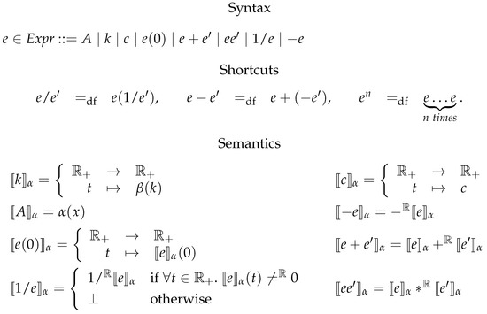
Figure 11.
Expressions where .
The semantics of expressions is parametrised by a function that interprets all parameters as positive real numbers. In order to simplify the notation, we assume that β is fixed, but notice that our simplification algorithms will be correct for any interpretation β.
The value of an expression is specified in Figure 11 for any variable assignment . It may either be a function of type or undefined ⊥. The latter is necessary for the interpretation of , which is defined only if for any time point t. We call an expression e nonnegative if is valid, i.e., if for all non-negative assignment α and all time points , we have .
Definition 8.
A kinetic expression is a nonnegative expression .
6.2. Constrained Flux Networks
The next objective is to add kinetic expressions to reactions and flux networks. Furthermore, we need to be able to express constraints about these kinetic expressions in order to express partial steady state hypothesis and conservation laws. This will lead us to the notion of constrained flux networks. A reaction with kinetics expressions is a pair where r is a reaction without kinetics and e is a kinetic expression. As before we now use flux reaction to represent a reaction but now with a kinetic expression.
Definition 9.
An n-ary flux reaction with kinetic expression is a pair composed of a vector and a kinetic expression . Given a tuple of reactions , the flux reaction represents the reaction .
The set of constraints on kinetic functions is defined in Figure 12. A constraint is a conjunction of atomic constraints. The first kind is an equation stating that the expressions e and must have the same value but different from ⊥. The atomic constraint requires that e is a constant function, that e may never becomes equal to zero, and that e is always non-negative. More formally, we define in Figure 12 the interpretation of a constraint for a given variable assignment α, where is the set of boolean values.
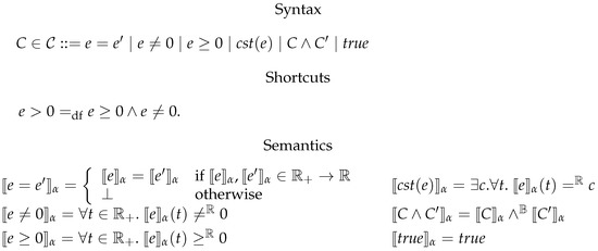
Figure 12.
Constraints on kinetic functions.
Definition 10.
An n-ary constrained flux network is a pair where V is a set of n-ary flux reactions with kinetic expressions and a constraint.
Let be a constrained flux network. We denote by the set of kinetic expressions e such that or such that e occurs in the constraint . We set:
6.3. Systems of Constrained Equations with ODEs
We now recall how to assign systems of equations to constrained flux networks. Note that systems constrained equations may contain both constraints and ordinary differential equations (Odes) in particular.
The set of systems of constrained equations is defined in Figure 13. They are conjunctions of constraints C and Odes where and . Note that the constraints may subsume the non-differential arithmetic equations . We denote by the set of (free) variables occurring in E, and by the set of expressions contained in E.
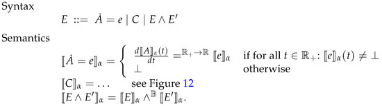
Figure 13.
Systems of constrained equations with Odes.
The denotation of a system of constrained equations E is a value in as defined in Figure 13. The set of solutions of is the set of assignments that make E true, i.e.,
We say that a constrained equation E logically implies another and write if . For instance, , , .
Definition 11.
Two constrained equation systems E and are called logically equivalent, denoted , if they have the same solutions, i.e.,
Clearly, if and only if E and logically imply each other, i.e., and .
6.4. Deterministic Semantics
We assign to any constrained flux network a system of constrained equations in Figure 14. Note that does depend on the tuple of initial reactions and the set of intermediates . The system contains an Ode for any species A stating that the change of the concentration of A is equal to the sum of the rates of the flux reactions . The factor makes the rate negative if A is consumed and positive if A is produced. It also takes care of the multiplicities of consumption and production. Finally, the constraint of the constrained flux network is added to the system of constrained equations.
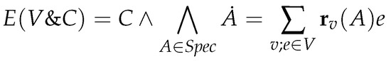
Figure 14.
System of constrained equations of a constrained flux network .
Example 5.
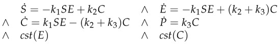
We consider the flux network for the classical Michaelis-Menten example [10]. Its system of constrained equations is then represented in Figure 15. It contains four ODEs and two constant constraints.
Figure 15.
System of constrained equations for Michaelis-Menten.
6.5. Contextual Equivalence
Two constrained flux networks W and are non-contextually equivalent, denoted , if their systems of constrained equations are logically equivalent:
We now extend the definition to a contextual equivalence. The idea is that networks can be exchanged with equivalent networks in any context, without affecting the semantics. As contexts, we use flux networks themselves . We define the combination of a network and the context as follows:
We now assume a set of intermediate species and call a context compatible if .
Definition 12.
Two constrained flux networks W and are (contextually) equivalent if they have the same solutions in any compatible context, that is:
We note that the definition of equivalence of constrained flux networks has two parameters: and . The equivalence ∼ depends on the tuple of initial reactions , since the non-contextual equivalence relation ≃ relies on the deterministic semantics of constrained flux networks, which in turn depends on . The equivalence relation ∼ also depends on the set of intermediates since the notion of compatibility depends on it.
Our simplification algorithm will rewrite constrained flux networks up to logical equivalence of constraints. Therefore, we can hope for confluence only up to logical equivalence. More formally, we defined the similarity relation ≅ as the least equivalence relation on constrained flux networks that satisfies the following two inference rules for all :
The first rule states that expressions that are logically equivalent under the constraints of the constrained flux network can be replaced by each other. The second rule allows to exchange logically equivalent constraints by each other. Similar networks are trivially equivalent:
Lemma 6.
Similarity implies contextual equivalence .
Proof.
Straightforward from the definitions. ☐
7. Simplification of Constrained Flux Networks
Our next objective is to simplify constrained flux networks by lifting the confluent simplification algorithm for flux networks to the case with kinetic expressions. This will require to impose partial steady state and linearity restrictions on the constrained flux networks, since otherwise, we would not know how to remove intermediates from the constrained equations assigned to the constrained flux network.
7.1. Linear Steadiness of Intermediate Species
The following restriction will allow us to eliminate an intermediate species from the constraint equations of a constrained flux network.
Definition 13.
We say that a species is linearly steady in a constrained flux network if it satisfies the following four conditions:
- Partial steady state: the concentration of X is steady, i.e., .
- Linear consumption: if a reaction in V consumes X then its kinetic expression is linear in X, that is: if such that then for some expression such that .
- Independent production: if a reaction in V produces X then its kinetic expression does not contain X except for subexpressions : for any , if then .
- Nonzero consumption: the consumption of X is nonzero: .
Suppose that X is linearly steady in . Since X is in partial steady state, we have and hence . The constrained equations of W thus imply that the production and consumption of X are equal:
The linear consumption of X imposes that for some expression e such that . The independent production of X imposes that . Because of nonzero consumption, we have:
where the expression does not contain the species X properly. Therefore, we can eliminate the variable X from the constrained equation by substituting X by . This give us hope that we can also eliminate linearly steady intermediate species from the constrained flux networks too by adapting the rule (F-Inter) to kinetic expressions.
7.2. Simplification
We now lift the simplification rules for flux networks to constrained flux networks. The lifted rules are presented in Figure 16. They define the simplification relation for constrained flux networks:
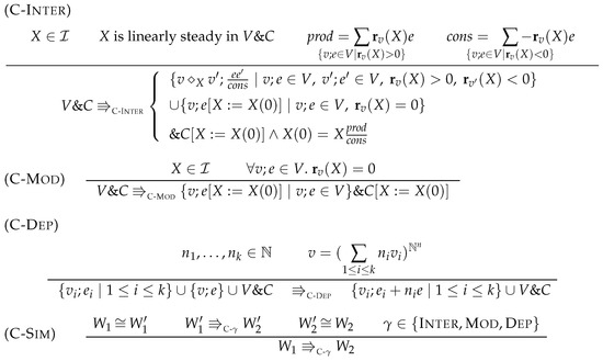
Figure 16.
Simplification rules for n-ary constrained flux networks, with the set of intermediate species and the n-tuple of initial reactions.
The first rule (C-Inter) eliminates a linearly steady intermediate species X, by merging any pair of reactions, so that the one produces and another consumes X. The rule can be applied only under the hypothesis that the constraints of the network imply that X is linearly steady, and so that X is in partial steady state in particular. It should also be noticed that the conditions on the initial value of X are preserved by the constraint . As argued above, the linear steadiness of X implies that the latter is equivalent to some other expression that does not contain species X properly. So except for constraints on the initial value , the species X got removed from the constrained flux network. The rule also replaces X by in all the kinetic expressions of reactions, in which X is used as a modifier, i.e., such that and . Furthermore, the same substitution is applied to the constraints of the flux network.
The rule (C-Mod) removes an intermediate that is never a reactant or a product of a reaction, and replaces X with its initial value . Then the rule (C-Dep) removes a dependent reaction. In contrast to the case without kinetics, the kinetic expressions of the remaining reactions need to be modified. The last rule (C-Sim) states that simplification is applied modulo similarity of constraint flux reaction networks.
The simplification defined here is sound for the contextual equivalence relation of constrained flux networks:
Proposition 2.
Given a constrained flux network W, if then .
The proof is given in Appendix C. The arguments are direct from the definitions, except that the Diamond Lemma 3 is needed in for .
7.3. Michaelis-Menten
We illustrate the simplification on the classical Michaelis-Menten example [10].
We consider the simplification of a three-step enzymatic scheme with mass-action kinetics into a single reaction with Michaelis-Menten kinetics. In the initial network, depicted in Figure 17, a substrate S can bind to an enzyme E and form a complex C. The complex can either dissociate back to S and E, or produce a product P, while releasing E. We assume here that the enzyme E and the complex C are intermediate species, i.e., they are at steady-state and cannot interact with the context. Therefore, the intermediate species E and C are linearly steady in this network.
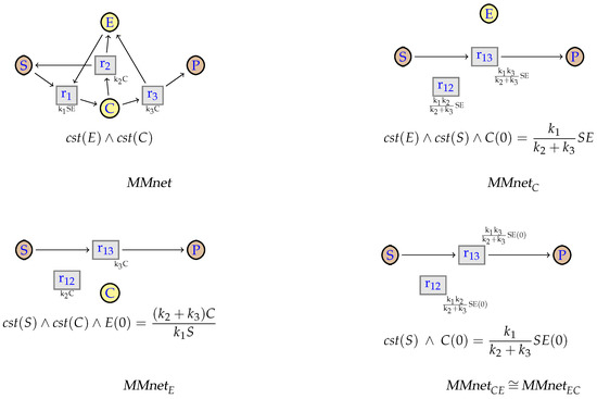
Figure 17.
Reaction networks for the Michaelis-Menten example. and are obtained from the initial network after removing E and C respectively. is obtained after removing both C and then E in this order. is obtained by inverting the order of elimination.
We first look at the elimination of the intermediate C with (C-Inter). To this end, we merge each reaction that produces C (that is, reaction ) with each reaction that consumes C (reactions and ) and obtain the network . Thus, merging reactions and (resp. and ) of (Figure 17) results in the reaction (resp. ) of . The simplification also replaces the atomic constraint with . Since we also have the constraint S, and the parameters are constant too, we can rewrite into the similar . We also add the constraint .
To remove E before the elimination of C, one would merge with , with , and obtain the network . At this point, in both networks we have an intermediate species that is neither a product nor a reactant of any reaction, but is used as a modifier. We can then remove it with (C-Mod), replacing E with (resp. C with ). We obtain respectively the networks and . Note that these networks are similar. We can rewrite into , and use this equation to rewrite the kinetic rate. Additionally, we can also use it to transform the kinetic expression of into the usual one for Michaelis-Menten, using the following transformation. First, we have:
We can then rewrite it into:
By replacing with this expression in the kinetic expressions of in , we obtain after basic rewriting the classical rate:
The following diagram illustrates the confluence of the simplifications on these networks.
8. Preservation of Linear Steadiness
As we have seen in the previous section, to remove an intermediate species X, we need to impose that X is linearly steady. When removing a set of intermediate species , we then need that any is linearly steady, and moreover than when we remove one intermediate species, the other species in remain linearly steady. We therefore introduce the following additional conditions, and denote by the set of networks that satisfy these conditions. We then prove that the set is stable under the simplification, i.e., that the simplification of a network in is still a network in .
8.1.
We first define the new conditions, and present some examples to motivate them. For any flux , we note and .
Definition 14.
We denote by the set of constrained flux networks W such that W is similar to a constrained flux network and that for all intermediates :
- 1.
- Either X is linearly steady in , or X is only a modifier, that is for any we have .
- 2.
- No intermediate species different from X occurs in the kinetic expression of a reaction that consumes X: for any , if , then .
- 3.
- The rate of a reaction that produces X but does not consume an intermediate species does not depend on the concentration of any intermediate species: for any , if and , then .
- 4.
- The total stoichiometry of the intermediate species in the reactant (resp. product) of a reaction is never greater than one: for any , and .
Note that, as a consequence of the stoichiometry condition, the sets and are either empty or consist of a single intermediate species.
We illustrate the motivations for these new conditions on the following examples.
Let us first consider the case where a reaction consuming X has a kinetic rate that depends on another intermediate (here Y in the kinetic rate of ), so that Condition 2 is not satisfied. It is illustrated in Figure 18.
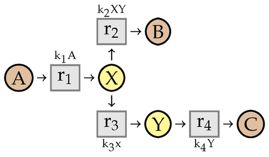
Figure 18.
Example illustrating the need of Condition 2.
If we remove Y first by merging and , then we compute the expression . We replace Y with this expression in the kinetic rate of , obtaining a reaction with a non-linear kinetic expression .
Similarly, consider a reaction producing X with a kinetic rate that depends on Y, i.e., a network where Condition 3 is not satisfied (Figure 19).
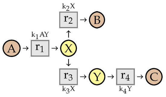
Figure 19.
Example illustrating the need of Condition 3.
If we remove the intermediate Y, the kinetic expression of becomes . We obtain a reaction producing X, with a kinetic expression depending on X. Therefore, the differential equation for X will not have the required form: , and we cannot compute an expression for X.
This kind of situation may also appear as the result of the simplification of reactions where one intermediate has a stoichiometry greater than one, i.e., Condition 4 is not satisfied (Figure 20).
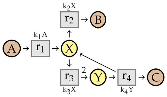
Figure 20.
Example illustrating the need of Condition 4.
In this network, reaction produces two molecules of Y. If we remove Y, the merging of and is a reaction that produces one molecule of X (and one of C), with kinetic expression .
Finally, if we have two intermediate species that are both reactants (or both products) in the same reactions (Condition 4 again), then the stoichiometry of one intermediate can become greater than one as a result of the elimination of the other intermediate (Figure 21).
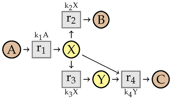
Figure 21.
Example illustrating the need of Condition 4.
If we remove Y, the merging of and is a reaction with two molecules of X as reactants.
8.2. Stability of
Now, we prove that is stable for our simplification.
We first consider the following proposition.
Proposition 3.
Let be reaction networks such that and . Let be a flux that depends on . Then:
- there exists an index i such that , , and
- for any , .
The proof of this proposition is quite long and requires some new notions and definitions, and is given in Appendix B.
We now prove that is stable for the simplification.
Proposition 4.
The set of networks is stable for the simplification, that is if and , then .
Proof.
If the simplification is done with (C-Mod) or (C-Sim), then the conditions of are trivially preserved.
Let us assume that the simplification is done with the rule (C-Dep), removing a flux that depends on with coefficient . So the simplified network contains the fluxes . By Proposition 3, there is an i such that and , and for any other , .
The fourth condition on the stoichiometry is trivially preserved by the simplification.
For , implies that the conditions on the kinetic expressions are directly satisfied. If consumes X, then since , the flux consumes X too. Then by induction, e and are linear in X, and no other intermediate species occurs in them. Therefore, this is also the case for .
If produces X without consuming any other intermediate, then it is also the case for . Then by induction, e, , and do not depend on the concentration of any intermediate species. Therefore, the kinetic conditions are satisfied, and .
Finally, consider the case of a rule (C-Inter) applied on a species X. We denote by and the expressions defined in the rule. Since , note that for any , we have .
Let be a reaction such that . We consider the second condition, on the linearity of Y in e. If (that is the flux has not been changed at all by the simplification rule), then the linearity condition is trivially preserved by induction. cannot be the simplification of a flux with X as modifier, since that would contradict the linearity condition in W. So now assume the is the merging of a flux and . Then we have and . Therefore, the linearity condition implies and , with for any , . Then we have , and the linearity condition is satisfied in .
Now let be a reaction such that and , and consider the third linearity condition. By linearity, cannot be the simplification of a reaction of W with X as modifier. If we had , then the condition is satisfied in W by induction, and therefore in too. Assume that is the merging of a reaction and . Then we have , , and . Therefore, the linearity conditions on W imply , with for any , . Then we have , and the condition is satisfied in .
Finally, consider the stoichiometric condition. We only have to verify this property for new fluxes that are the merging of a flux and . We have . Moreover, by normalization, we have
Since , we have , and similarly for . ☐
Then the set is stable for the simplification. This directly implies that the simplification can remove every intermediate species in .
9. Confluence of the Simplification Relation
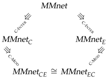
We now study the confluence of the simplification relation. We first show that the structural confluence, that is the confluence of the fluxes without kinetics, is a direct consequence of the previous results. We next present an example that illustrates that, however, the distribution of the kinetics between the fluxes can be different. Finally, we give a criterion on the modes of a network, that guarantees the full confluence, that is confluence of the structure and the rates.
In the following, we only consider networks in .
9.1. Structural Confluence
We say that two constrained flux networks and are structurally similar, denoted , if they have the same structure, that is the same fluxes when neglecting the kinetic expressions:
Theorem 3 (Structural confluence).
The relation on is confluent.
Proof.
This is a direct consequence of the stability of the (Proposition 4) and of the confluence of the simplification without kinetics (Theorem 2). ☐
9.2. Non-Confluence of the Kinetic Rates
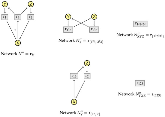
Let us consider the reaction network W, depicted on Figure 22, with 7 species and 6 fluxes. The intermediate species are X, Y and Z. Initially, the kinetics are all mass-action.
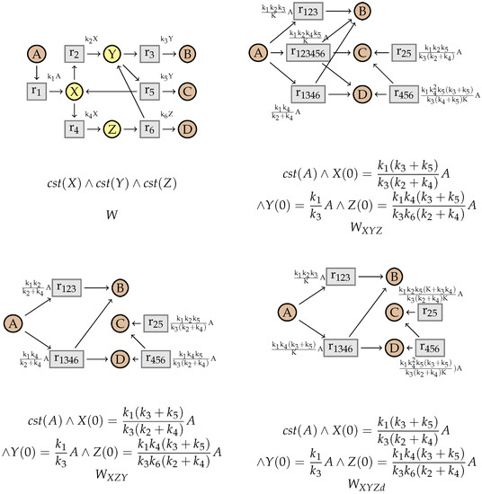
Figure 22.
Network W and its simplifications. (top left) Network W. (top right) Network after eliminating X, Y and Z (in this order). (bottom left) Network after eliminating X, Z and Y. (bottom right) Network after eliminating X, Y, Z, and the dependent reaction. The new parameter is .
We can remove the intermediate species in different orders with (C-Inter). If we start by eliminating X, followed by Y and finally Z, we obtain the network , while if we first eliminate X, then Z and Y, we obtain . These networks are different, since has one additional flux. This illustrates the necessity of the rule (C-Dep) to obtain the same network structure.
Indeed, the additional flux in is dependent on and and can therefore be removed with (C-Dep), while updating the kinetic expressions. We then obtain exactly the network . However, also depends on and . Therefore, we could as well remove it while updating these reactions. In that case, we obtain the different network . This network has the same structure as , but not the same distribution of rates between the fluxes.
9.3. Criterion for the Full Confluence
We now give a criterion that guaranties the full confluence of the simplification.
Definition 15.
A vector of reactions is uniquely decomposable if any mode has an unique decomposition in elementary modes, where S is the stoichiometric matrix of .
Example 6.
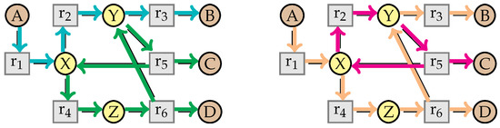
Consider the network W represented in the Figure 22, with . It has 4 different elementary modes: , , and . Then the mode can be decompose in either , or in . The two decompositions are illustrated in Figure 23. is not uniquely decomposable, and the simplification is not confluent for the kinetic rates, as we have seen before.
Figure 23.
Two decompositions of the mode in the network W.
Theorem 4 (Confluence).
If the initial vector of reactions is uniquely decomposable, then the relation on is confluent, for both the structure and the kinetic rates.
The theorem is the consequence of the following lemmas, that analyze the different critical pairs. That is, if a network W can be simplified in two different manners into and , then these two networks can be simplified into and such that .
Lemma 7.
Assume is uniquely decomposable. Let W be a network such that for . Then such that and .
Proof.
Let be the dependent flux removed when simplifying W into , for , with dependent on with coefficients .
If , since is uniquely decomposable, we have . So the simplified networks are trivially the same, that is .
Assume , and that for any , for any j, , that is does not depend on and reciprocally. Then we can still remove in , and in , and we find the same network modulo similarity: .
If depends on , and depends on , then since dependencies are positive linear combinations, that directly implies .
Finally, if , and depends on , with coefficient a, but does not depend on (or conversely), we have and . If we remove , becomes , and can be removed. The fluxes obtained are of the form . If we remove first, then we can remark that is still dependent, with , and can be removed. We obtain the fluxes . Then the simplified fluxes are similar, and . ☐
Lemma 8.
Let W be a network such that and . Then such that and .
Proof.
This case is quite trivial. Let be the dependent flux, X the modifier, and another reaction such that v depends on with factor a. If we remove X first and then v, the flux is simplified into . Otherwise, it is simplified into . The two expressions are trivially similar. ☐
Lemma 9.
Let W be a network such that and . Then such that and .
Proof.
The full proof is given in Appendix C. The main idea is to use Proposition 3 to prove that if X is in the dependent flux , it is also in one of the fluxes that depends on. Therefore, if we eliminate X and combine with another flux , we also merge with . Then is still dependent on and other fluxes, and can be removed. ☐
Lemma 10.
Let W be a network such that for . Then such that and .
Proof.
This case is trivial, since the substitutions commute. ☐
Lemma 11.
Let W be a network such that and . Then such that and .
Proof.
Once again, since the two removed species cannot be the same, this case is trivial. ☐
Lemma 12.
Let W be a network such that for . Then such that and .
Proof.
The full proof is given in Appendix C. The idea is that after removing one intermediate species, we can still remove the other one, either with (C-Mod) or with (C-Inter). In the second case, some dependent fluxes are generated, that we can eliminate to find the same simplified network, whatever the order of elimination of the intermediate species. ☐
10. An Example from the BioModels Database
We have shown that the simplification system that we presented can exhibit non-confluence of the rates, even in a simple scenario with a small number of intermediates. To find if such a situation occurs in practice, we investigated the SBML models in the curated BioModels database [6]. We were thus able to find a network, for the model BIOMD0000000173, that does not verify the confluence criterion, and such that two different simplified networks can be identified. Note that this was the only model not satisfying the criterion, when considering every model of the BioModels database with mass-action kinetics and with three or four linear intermediate species.
The network identified is a model of the -based signal transduction mechanisms from the cell membrane to the nucleus, presented in [23]. We only consider here a sub-network W of this model, sufficient to illustrate the non-confluence. It is represented in Figure 24.
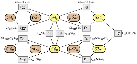
Figure 24.
Sub-network W of the -based signal transduction model from [23].
In this network, a molecule of , that represents the species in the cytoplasm, can bind with either a molecule of in a phosphorylated form () and form the complex (reaction ), or with a molecule of G in a phosphorylated form (), and form the complex (reaction ). These two reactions are reversible ( and ). The same transformations can occur in the nucleus (reactions , , and ). The species can also move from the cytoplasm to the nucleus, or reciprocally ( and ). Finally, the complex of and can move from the cytoplasm to the nucleus ().
We assume that . The network is in . Therefore, we can consider the elimination of the four intermediate species. According to the order of the simplification, we can then obtain two different networks, with the same structure, but with different kinetic expressions. They are represented in Figure 25. The network is obtained by removing first, then , then , and finally and the dependent fluxes. The network is obtained by removing , then , , and the dependent fluxes.
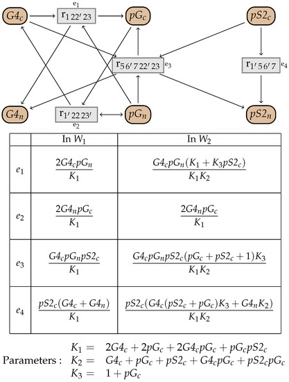
Figure 25.
Simplified networks from W. Both networks have the same structure, and the kinetic expressions are defined in the table. The network is obtained by removing in order , , , and the dependent fluxes. The network is obtained by removing in order , , , and the dependent fluxes.
We now show that the criterion is not satisfied in the initial network, i.e., that W is not uniquely decomposable. We consider the following mode:
This mode has two possible decompositions into elementary modes, and , with:
We represent these fluxes in Figure 26, where we omit the non-intermediate species and the kinetic expressions for the sake of simplicity.
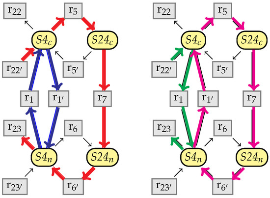
Figure 26.
In red the elementary mode , in blue , in green , and in magenta .
11. Simplification of Systems of Equations
In this section, we study the relation between the simplification on reaction networks and a simplification ⇒ on systems. We show that the assignment of a system to a network W is a simulation for the simplifications.
11.1. Simplification of Systems of Equations
The simplification of systems is illustrated in Figure 27. The first rule replaces a constant variable x with its initial value , and with 0. The second rule extends the simplification to similar systems. We define the simplification:
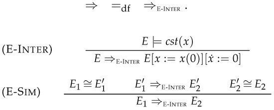
Figure 27.
Simplification rules for systems of equations.
Lemma 13.
The simplification is correct for the equivalence, that is:
Theorem 5.
The relation ⇒ on is uniformly confluent.
Proof.
It is trivial, since the substitutions commute. ☐
11.2. Simulation
The assignment of a system to a network W is a simulation from to .
Lemma 14.
Given a network , if , then .
Proof.
The rule (C-Sim) for the networks is directly imitated by the rule (E-Sim) for the systems.
For the rule (C-Mod), if , then we directly have .
For the rule (C-Inter), assume that we remove a species X from W to obtain . Then , therefore, we can simplify into a system . We have to prove that . First, observe that the systems have the same variables.
Consider a differential equation of , for a species :
We define and . The differential equation in becomes:
| = | ||
| = | ||
| = | ||
| = | ||
| = | . |
The system also contains the constraint . In addition, by the linearity conditions, we know that for any such that , we have , so . For any such that , we have , with . Therefore, . So we can rewrite the previous differential equation into:
In , we directly have
Moreover, in , the equation is replaced by . We then have , while for some e such that . Then . So we can rewrite the equation into , and then into . Therefore, the two systems and have the same differential equations and the same constraint, and they are similar.
Finally, consider the rule (C-Dep). Let be the removed reaction, depending on , with coefficients . We write for the set of the other fluxes in W. Let A be a species. The ordinary differential equation for A in is:
Since we have , the equation is similar to:
This is the equation for A in the system for the simplified network. Therefore, . ☐
12. Conclusions
We have first shown that when neglecting the kinetic expressions, the elimination of linear intermediate species and dependent reactions is a reformulation of the double description method, that computes the elementary modes, and therefore that the network structure of simplified networks is unique. In a second time, when considering kinetic expressions, we provided a biological example illustrating that the simplification can produce two networks with the same structure but different kinetics. We then gave a sufficient criterion on the network structure of the initial network that guarantees the confluence of both the structure and the rates.
Note that the criterion seems to be satisfied in most cases in practice. When looking at the networks with mass-action kinetics from the BioModels database [6], and considering at most four intermediate species, only the -model BIOMD0000000173 was identified as not satisfying the criterion. On the other hand, the linearly steadiness as well as the conditions required for a network to be in (such as the stoichiometry conditions, etc.) are not always satisfied in real biological networks, and these are therefore a real restriction on our simplification approach.
Acknowledgments
This work has been funded by the French National Research Agency research grant Iceberg ANR-IABI-3096.
Author Contributions
All authors contributed equally to this work and to the writing of the paper.
Conflicts of Interest
The authors declare no conflict of interest.
Appendix A. Soundness of the Simplification Rules for Constrained Flux Networks
We prove Proposition 2, stating that the simplification is sound for the congruence: implies .
We prove, for each simplification rule, that for any context with and for any assignment α, we have iff . Let us assume that , , and . We therefore have
where
(C-Mod) Suppose that the removed species is . Since for any , and . Moreover, , thus and the ODE for X in is , which is also the equation for X in . As a consequence any solution α should verify . In addition, since and only differ by the substitution of for X, they have the same solutions.
(C-Dep) Let where , i.e., v depends on with coefficients . For any species A, we can write its ODE in as
which is exactly the ODE for A in . In addition, the constraints in and are the same. Therefore, their solutions are identical.
(C-Sim) The soundness of this rule comes directly from Lemma 6.
(C-Inter) Suppose that the removed species is . We note that .
Let and be such that . Let P, C, , and be as in the Diamond Lemma 3, with the set of kinetic expressions, for all , and the homomorphism with . P is the set of indices for fluxes that produce X, C the set of indices for fluxes that consume X, while is the total rate of production of X, and its total rate of consumption.
The Ode for X in is . Since X is linearly steady in W, it follows that . Therefore, we have that . Let be a species. The Ode for A in writes as
We next consider the Ode for A in and show that it can be rewritten to obtain the same result. We have
Without the substitution , this is indeed the equation of A in . The substitution is permitted since we argue modulo similarity of constrained flux networks, and since . Therefore, so that .
Appendix B. Proofs for the Stability of LinNets
We first need to introduce some new notions.
We write for the initial vector of reactions, and for the corresponding unit vectors, that is, for any i, . Let be a constrained flux network, and W a network obtained by simplifying , that is .
We first introduce the notion of paths. We will then relate them to the fluxes in W. Note that we need to distinguish between the case of circular and the case of non-circular path.
Definition A1.
Let be the initial vector of reactions.
- a path is a (non empty) sequence of unit vectors , such that for any , we have ;
- we denote the vector of a path by ;
- a path is circular if , and non-circular otherwise;
- for a circular path , we denote the number of intermediate species occurring in the path by ;
- for a non-circular path , we denote its beginning and its end by and . In addition, we define the multiset . Note that we do not count and in this multiset.
Example A1.
For instance, consider the initial network , with , in Figure A1 (left). We denote by the unit vector for reaction .
The path is non-circular. It has for vector . We have and . The multiset is defined by , and (since Z is the end of the path, and not an intermediate node).
The path is circular. It has for vector . The multiset is defined by and .
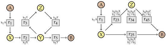
Figure A1.
Networks (left); and W (right).
We will see later that if a path satisfies some conditions w.r.t. some reaction network W, then there is a corresponding flux v in W such that . The reciprocal property also holds. Such a particular path, called a flux-path, is formally defined as follows.
Definition A2.
Let be reaction networks such that ,
- a non-circular flux-path is a non-circular path in W such that for any intermediate species X with , we have (meaning that one of the simplification steps removes X from ), and such that and are either the empty solution ∅, or the intermediate species that are still in W,
- a circular flux-path is a circular path in W if there is at most one intermediate species X such that and (i.e., X is not yet simplified),
- we call flux-path a path that is either a circular or a non-circular flux-path.
- a flux-path is said to correspond to a flux v in W if .
Example A2.
Let us consider the simplified network W in Figure A1 (right).
The non-circular path is not a non-circular flux-path, since and X has not been removed. The path is a non-circular flux-path, and corresponds to the flux .
The path is a circular flux-path, since there is a unique intermediate species, Z, that has not been removed and such that . It corresponds to .
We first prove the following lemma on the dependent flux.
Lemma A1.
Let be a flux that depends on with coefficients . For any i, let be a corresponding flux-path for . Then:
Proof.
We directly have and for any i, . ☐
We can now prove the key lemma of this section.
Lemma A2.
Let be reaction networks such that and . Then the following properties hold:
- 1.
- for any flux , there is a corresponding flux-path for W such that . Moreover, if v is not dependent then, for any intermediate species X, we have ;
- 2.
- for any flux-path for W such that for any X, , there is a corresponding flux , that is ;
- 3.
- if depends on , then
- there exists an index i such that , , and
- for any , and any flux-path that corresponds to v is circular.
Proof.
We proceed by induction on the simplification steps. We start by proving each conclusion of the Lemma for the base case, that is .
- (1)
- for flux in the initial network , v is necessarily a unary vector for some i. So we can directly associate the flux-path that trivially corresponds to v. Since it is a unary vector, the flux v is also necessarily not dependent. Because a flux-path of size 1 is always non-circular, we also have, for any intermediate species X, , and thus as required.
- (2)
- any flux-path for is necessarily of size 1. Otherwise, for being a non-circular flux-path, there would exist some . And for being a circular flux-path, there would exist at least two species X and Y such that and , which contradicts the definition of circular flux-path. Then there exists such that .
- (3)
- as said above, a flux v can not be dependent.
Now, considering the inductive case, we assume that the Lemma is true for a network such that (for some ) and . If or , only the kinetics are modified between and W. Therefore, the Lemma is still true in W. It remains to investigate the cases and .
(C-Dep) Assuming that , we prove that each point of the Lemma is satisfied by W.
- (1)
- Let , then it is the case that for some expression because the rule (C-Dep) only removes a dependent flux and modifies some kinetic expressions. By induction hypothesis, there is a flux-path for such that . Also, because , any flux-path for is also a flux-path for W, which proves that is a flux-path for v. Finally, if v is dependent in W, it is necessarily dependent in W and satisfies by induction hypothesis.
- (2)
- Let be a flux-path for W such that, for any intermediate species X, . Again, because , is also a flux-path for . By induction hypothesis, there is a corresponding flux . If is not the flux that is removed by the application of (C-Dep), then this flux still occurs in W (possibly with an updated kinetic) and we conclude directly. We now show that it can not actually be otherwise, and more precisely, that assuming v removed by (C-Dep) contradicts .Suppose that v is removed by (C-Dep), then v depends on some fluxes in . For the sake of simplicity, we only consider the case where for some intermediate . The other case works similarly. We necessarily have , because contradicts the linearity assumption. By induction hypothesis and Point 3, there exists in particular at least one j such that . Again, by induction hypothesis, there exists a circular flux-path corresponding to in . Since it is circular, there exist some intermediate species such that for any , and , and , . Note that we also have , since, by definition of flux-path, for any i, while . Since and , the unit vectors also appear in the flux-path . So the intermediate species are present at least one time in . Moreover, there is at least one i such that in , the unit vector is preceded by a unit vector that is not one of . Therefore, is produced by another flux, i.e., , which contradicts the hypothesis.
- (3)
- Let be a flux dependent on , that is, in particular, for some . Since (C-Dep) removes one flux and possibly modifies some kinetics, there is a flux in that either depends on or on where is the flux removed by (C-Dep). The latter case is not possible, since it would imply that for some and unary vector . Thus, we conclude that depends on that, by induction hypothesis, satisfies the conditions of Point 3.
(C-Inter) Now, assuming that , we again prove that each point of the Lemma is satisfied by W.
- (1)
- Let be in W. Either there is a corresponding flux , and we conclude directly by induction hypothesis, or is the result of merging some that produces X and some that consume it. In this case, by induction hypothesis, there are some corresponding flux-paths and . The concatenation of these paths is a flux-path. Indeed,
- the production of coincides with the consumption of because there is an intermediate species X such that , and .
- if is non-circular, for any intermediate species Y such that , either and , or, or and by induction hypothesis, that is .
- if is circular, there exists an intermediate species Y which is both consumed by and produced by . The flux-path cannot be circular, as this would imply , and similarly for . By definition of non-circular flux-path, X and Y are the only two species in and such that and . Thus, Y is the only non-eliminated intermediate species in w.r.t. W, meaning again that is indeed a circular flux-path.
Moreover, trivially corresponds to v. We prove with Point 3 that if is non-dependent, then for any X. - (2)
- Let be a flux-path for W such that for any Y, . Let X be the intermediate species removed by (C-Inter), in particular , hence either or . Since , if , then is also a flux-path for , so by induction there is a corresponding flux . Since , we still have a flux , that corresponds to . If then we can decompose into producing X and consuming X such that . and can not be circular, as this would imply that X is both consumed and produced by and by , contradicting the fact that . Therefore . Again, because and X is the species removed by (C-Inter) and is a flux-path, and are (non-circular) flux-paths for . We can then apply the induction hypothesis and infer that there are some corresponding fluxes , the first one that produces X and the second one that consumes it. Consequently, there is a flux that is the merging of and , and that corresponds to .
- (3)
- Let be a flux that depends on and X be the intermediate species removed by (C-Inter). We distinguish two cases: either (case 1) is the simplification of some flux (meaning that v does neither produce nor consume X) or (case 2) it results from merging fluxes that produce and consume X.(Case 1) By induction hypothesis and Point 1, there exists a flux-path corresponding to v for . We have since X has not been removed. Suppose that there is such that is the merging, by (C-Inter), of fluxes that produce and a consume X. In this case, for any corresponding to , and, by the Lemma A1, we would have that , which contradicts . Therefore, none of the s are the merging of other fluxes by (C-Inter), therefore, there are such that depends on those fluxes. Since, by induction hypothesis, Point 3 is satisfied for in , it is also satisfied for in W.(Case 2) Let be a flux that produces X, and a flux that consumes it and their merging. Let and be flux-paths in for, respectively, and (such flux paths exist by induction hypothesis). Any corresponding path is then the concatenation of corresponding paths and .We first prove that, if either or is dependent in , then is also dependent in W. By induction, if depends on , there exists a unique i such that , , and, for any , . Then, there is a flux in W that is the merging of and , and there are fluxes in W for . Then depends on and the .If both and are not dependent, by induction hypothesis, for any , in the corresponding flux-path, we have and . If , then . We also have (indeed, X is the removed species, so and the X produced by is merged with the X consumed by in ). Therefore, in this case Point 1 is satisfied. If there is a Y such that , then Y occurs twice in , and there is an intermediate species Z (that can possibly be Y if no other intermediate species occurs more than once between both occurrences of Y) such that and such that there is a circular flux-path , subpath of that begins and end with Z:
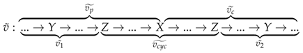 Then using Point 2, there is a corresponding flux , with . We can repeat the same operation on the remaining path , and obtain at each step a new (circular) flux. We stop when we obtain a remaining path , such that for any Y, we have . Then there is a corresponding flux with , and . Then v is dependent on and the set of circular fluxes we obtained in this process. Therefore, in this case Point 3 is satisfied.Now assume that and are dependent, and so that is dependent too. By induction and using Point 3, depends on a flux with and , and on other fluxes such that , and similarly for . Then any and any is still in W, while is merged with , forming a new flux . Then depends on , the and the . Since , and similarly , Point 3 is satisfied.
Then Proposition 3 is a direct corollary of Point 3 of Lemma A2.
Appendix C. Proofs of the Full Confluence of the Simplification
We prove Lemmas 9 and 12.
Lemma A3.
Let W be a network such that and . Then such that and .
Proof.
Let X be the intermediate species, and the dependent reaction, that depends on , with coefficients .
The main idea is to use the Proposition 3 to prove that if X is in the dependent flux , it is also in one of the fluxes whose depends on. Therefore, if we eliminate X and combine with another flux , we also merge with . Then is still dependent on and other fluxes, and can be removed.
Let us first assume that X is not involved in (that is, ). By Lemma A2, Point 3, X is not involved in the either. Then will still be dependent in , so we can still remove it after removing X. Reciprocally, X can still be removed in . We now show that the simplification of the fluxes are the same in and . The case for the other fluxes is trivial. In , we obtain the flux . In , we obtain . Therefore, these two expressions are similar, and .
Assume that , for instance . Then, again by Lemma A2 and Point 3, there is a flux with , and for any other , . We denote by and the expressions as defined in the rule (C-Inter), by the fluxes that produce some X, and the ones that consume it.
In after removing X, we obtain the fluxes:
- the combination of and the consuming fluxes: ,
- the combination of and the consuming reactions: ,
- the other combined fluxes: ,
- the remaining fluxes not combined: ,
- the other fluxes that are not in , , , where we substitute X by .
Since was dependent on , we have that any flux in the first set is dependent on a flux in the second set and the fluxes . Therefore, we can recursively remove those fluxes with the rule (C-Dep). We obtain the network with the fluxes:
- ,
- ,
- ,
- the other fluxes that are not in , , , where we substitute X by .
Now, if we first remove , in we obtain the fluxes:
- ,
- ,
- the other fluxes that are not in , , .
We can still remove X, we obtain the reactions:
- ,
- ,
- ,
- the other fluxes that are not in , , , where we substitute X by .
Note that we have:
The fluxes of the two simplified networks are therefore similar, that is . The case with is similar. ☐
Lemma A4.
Let W be a network such that for . Then such that and .
Proof.
The main idea here is that after removing one intermediate species, we can still remove the other one, either with (C-Mod) or with (C-Inter). In the second case, some dependent fluxes are generated, that we can eliminate to find the same simplified network, whatever the order of elimination of the intermediate species.
Let X and Y be the intermediate species removed to obtain and . We can partition the fluxes of W into:
- , the fluxes producing X without Y,
- , the fluxes consuming X without Y,
- , the fluxes with modifier X and without Y,
- , the fluxes producing Y without X,
- , the fluxes consuming Y without X,
- , the fluxes with modifier Y and without X,
- , the fluxes producing X and consuming Y,
- , the fluxes producing Y and consuming X,
- , the fluxes with modifier X and Y.
We define the following variables:
Let first remove X. We obtain the following combined fluxes:
- ,
- ,
- ,
- .
The fluxes with X as modifier become (with :
- ,
- .
Finally, some fluxes are not modified:
- ,
- ,
- .
There are now two cases to consider. First, it is possible that Y is now only a modifier in . This means that , that is any flux with X as reactant (resp. product) also admits Y as product (resp. reactant), and reciprocally. We can then apply (C-Mod) on , and obtain the fluxes (with ):
- .
- ,
- ,
- .
Using the constraint to rewrite the first kinetic expression into , we can see by symmetry that we obtain similar fluxes by removing Y first (with (C-Inter)) and then X (with (C-Mod)).
In the other case, we can still remove Y with (C-Inter). We first compute the sum (resp. ) of the kinetics of the fluxes that produced (resp. consumed) Y:
We write . We obtain the following combined fluxes:
- ,
- ,
- ,
- .
The fluxes with Y as modifier become:
- ,
- ,
- ,
- .
Finally, some fluxes do not involve Y:
Now we can observe that we obtained some dependent fluxes. Any flux in is the combination of a flux from and . We can then remove the first flux, while modifying the kinetics of the others. Finally, after simplifying the kinetic expressions by similarity, the simplified network has the following fluxes:
- ,
- ,
- ,
- ,
- ,
- ,
- ,
- ,
We can observe that:
- the 2 first sets are symmetric to each other, in the sense that if we switch X and Y in the first set, we obtain the second one,
- the 2 following sets are symmetric to each other,
- the 2 following sets are symmetric to each other too,
- the following set is symmetric in X and Y,
- the last set is symmetric in X and Y (since the substitutions commute).
Therefore, by symmetry, we can obtain exactly the same network if we first remove Y, then remove X and the dependent fluxes. We conclude that .
☐
References
- Feinberg, M. Chemical reaction network structure and the stability of complex isothermal reactors—I. The deficiency zero and deficiency one theorems. Chem. Eng. Sci. 1987, 42, 2229–2268. [Google Scholar] [CrossRef]
- Hucka, M.; Finney, A.; Sauro, H.M.; Bolouri, H.; Doyle, J.C.; Kitano, H.; Arkin, A.P.; Bornstein, B.J.; Bray, D.; Cornish-Bowden, A.; et al. The systems biology markup language (SBML): A medium for representation and exchange of biochemical network models. Bioinformatics 2003, 19, 524–531. [Google Scholar] [CrossRef] [PubMed]
- Calzone, L.; Fages, F.; Soliman, S. BIOCHAM: An environment for modeling biological systems and formalizing experimental knowledge. Bioinformatics 2006, 22, 1805–1807. [Google Scholar] [CrossRef] [PubMed]
- Kuttler, C.; Lhoussaine, C.; Nebut, M. Rule-based modeling of transcriptional attenuation at the tryptophan operon. In Transactions on Computational Systems Biology XII; Springer: New York, NY, USA, 2010; pp. 199–228. [Google Scholar]
- Chaouiya, C. Petri net modelling of biological networks. Brief. Bioinform. 2007, 8, 210–219. [Google Scholar] [CrossRef] [PubMed]
- Juty, N.; Ali, R.; Glont, M.; Keating, S.; Rodriguez, N.; Swat, M.J.; Wimalaratne, S.M.; Hermjakob, H.; Le Novère, N.; Laibe, C.; et al. BioModels: Content, Features, Functionality and Use. CPT Pharmacomet. Syst. Pharmacol. 2015, 4, 55–68. [Google Scholar] [CrossRef] [PubMed]
- Mäder, U.; Schmeisky, A.G.; Flórez, L.A.; Stülke, J. SubtiWiki—A comprehensive community resource for the model organism Bacillus subtilis. Nucleic Acids Res. 2012, 40, 1278–1287. [Google Scholar] [CrossRef] [PubMed]
- Niehren, J.; John, M.; Versari, C.; Coutte, F.; Jacques, P. Qualitative Reasoning about Reaction Networks with Partial Kinetic Information. In Computational Methods for Systems Biology; Lecture Notes in Computer Science; Springer: New York, NY, USA, 2015; Volume 9308, pp. 157–169. [Google Scholar]
- Radulescu, O.; Gorban, A.N.; Zinovyev, A.; Noel, V. Reduction of dynamical biochemical reactions networks in computational biology. Front. Genet. 2012, 3, 131. [Google Scholar] [CrossRef] [PubMed]
- Michaelis, L.; Menten, M.L. Die kinetik der invertinwirkung. Biochem. Z. 1913, 49, 333–369. (In German) [Google Scholar]
- Segel, L.A. On the validity of the steady state assumption of enzyme kinetics. Bull. Math. Biol. 1988, 50, 579–593. [Google Scholar] [CrossRef] [PubMed]
- Cornish-Bowden, A. Fundamentals of Enzyme Kinetics; Wiley: Hoboken, NJ, USA, 2013. [Google Scholar]
- Heineken, F.; Tsuchiya, H.; Aris, R. On the mathematical status of the pseudo-steady state hypothesis of biochemical kinetics. Math. Biosci. 1967, 1, 95–113. [Google Scholar] [CrossRef]
- Segel, L.A.; Slemrod, M. The quasi-steady-state assumption: A case study in perturbation. SIAM Rev. 1989, 31, 446–477. [Google Scholar] [CrossRef]
- King, E.L.; Altman, C. A schematic method of deriving the rate laws for enzyme-catalyzed reactions. J. Phys. Chem. 1956, 60, 1375–1378. [Google Scholar] [CrossRef]
- Chou, K.-C.; Forsen, S. Graphical rules of steady-state reaction systems. Can. J. Chem. 1981, 59, 737–755. [Google Scholar]
- Fages, F.; Gay, S.; Soliman, S. Inferring reaction systems from ordinary differential equations. Theor. Comput. Sci. 2015, 599, 64–78. [Google Scholar] [CrossRef]
- Sáez, M.; Wiuf, C.; Feliu, E. Graphical reduction of reaction networks by linear elimination of species. J. Math. Biol. 2017, 74, 195–237. [Google Scholar] [CrossRef] [PubMed]
- Madelaine, G.; Lhoussaine, C.; Niehren, J. Attractor Equivalence: An Observational Semantics for Reaction Networks. In Formal Methods in Macro-Biology; Springer: New York, NY, USA, 2014. [Google Scholar]
- Schmidt-Schauss, M.; Sabel, D.; Niehren, J.; Schwinghammer, J. Observational Program Calculi and the Correctness of Translations. J. Theor. Comput. Sci. 2015, 577, 98–124. [Google Scholar] [CrossRef]
- Gagneur, J.; Klamt, S. Computation of elementary modes: A unifying framework and the new binary approach. BMC Bioinform. 2004, 5, 175. [Google Scholar] [CrossRef] [PubMed]
- Madelaine, G.; Lhoussaine, C.; Niehren, J.; Tonello, E. Structural simplification of chemical reaction networks in partial steady states. Biosystems 2016, 149, 34–49. [Google Scholar] [CrossRef] [PubMed]
- Schmierer, B.; Tournier, A.L.; Bates, P.A.; Hill, C.S. Mathematical modeling identifies Smad nucleocytoplasmic shuttling as a dynamic signal-interpreting system. Proc. Natl. Acad. Sci. USA 2008, 105, 6608–6613. [Google Scholar] [CrossRef] [PubMed]
© 2017 by the authors. Licensee MDPI, Basel, Switzerland. This article is an open access article distributed under the terms and conditions of the Creative Commons Attribution (CC BY) license ( http://creativecommons.org/licenses/by/4.0/).