A Physics-Informed Neural Network Aided Venturi–Microwave Co-Sensing Method for Three-Phase Metering

Abstract

Addressing the challenges of online measurement of oil-gas-water three-phase flow under high gas–liquid ratio (GVF > 90%) conditions (fire-driven mining, gas injection mining, natural gas mining), which rely heavily on radioactive sources, this study proposes an integrated, radiation-source-free three-phase measurement scheme utilizing a “Venturi tube-microwave resonator”. Additionally, a physics-informed neural network (PINN) is introduced to predict the volumetric flow rate of oil-gas-water three-phase flow. Methodologically, the main features are the Venturi differential pressure signal ($\mathrm{\Delta }P$) and microwave resonance amplitude ($V$). A PINN model is constructed by embedding an improved L-M model, a cross-sectional water content model, and physical constraint equations into the loss function, thereby maintaining physical consistency and generalization ability under small sample sizes and across different operating conditions. Through experiments on oil-gas-water three-phase flow, the PINN model is compared with an artificial neural network (ANN) and a support vector machine (SVM). The results showed that under high gas–liquid ratio conditions (GVF > 90%), the relative errors (REL) of PINN in predicting the volumetric flow rates of oil, gas, and water were 0.1865, 0.0397, and 0.0619, respectively, which were better than ANN and SVM, and the output met physical constraints. The results indicate that under current laboratory conditions and working conditions, the PINN model has good performance in predicting the flow rate of oil-gas-water three-phase flow. However, in order to apply it to the field in the future, experiments with a wider range of working conditions and long-term stability testing should be conducted. This study provides a new technological solution for developing three-phase measurement and machine learning models that are radiation-free, real-time, and engineering-feasible.

1. Introduction

Oil-gas-water three-phase flow is widely present in fields such as oil and gas extraction, chemical processes, and nuclear reactors. Its complex flow characteristics and interphase interactions make accurate measurement of flow rate and phase holdup a major challenge in engineering applications. Especially under high gas–liquid ratio conditions, traditional measurement methods often face issues such as low accuracy and poor adaptability. Therefore, the development of high-precision, real-time online three-phase flow measurement technology holds significant theoretical and engineering value.

Multiphase flow measurement technology has evolved from separation methods to non-separation methods. Traditional complete separation methods and split-flow phase separation methods measure three-phase flow by separating it into single-phase fluids and metering them separately [1]. However, this method is not only costly and bulky but also unable to reflect the actual flow state at the wellhead or pipeline in real time. With technological advancements, non-separation methods have emerged, with representative methods including electromagnetic flow meters, ultrasonic methods [2], conductivity methods [3], radio frequency methods, etc. These methods have overcome the shortcomings of separation methods to some extent, but under conditions such as high gas–liquid ratios and complex flow patterns, they still face issues of insufficient measurement accuracy and adaptability [4].

The Venturi tube, as a traditional differential pressure flow meter, is widely used for flow measurement of wet gas two-phase flows. In 2014, Monn [5] established a model for the pressure difference and irreversible pressure loss generated by two-phase flows passing through a Venturi tube and achieved two-phase flow measurement for high-void-fraction annular flows through an iterative solution. The evaluation accuracy of mass flow rates for air and water was better than 2% and 30%, respectively. In 2015, Yuan Chao et al. [6], based on dimensional analysis, established a wet gas high void fraction model using parameters such as differential pressure ratio $K,$ ${\rho }_g/{\rho }_l$, and ${Fr}_g$. This model demonstrated good measurement performance both in the laboratory and in industrial sites. In 2019, Luo Yi et al. [7] conducted experimental verification on Venturi tubes with different tube diameter ratios and found that the Venturi tube with a tube diameter ratio of 0.55 exhibited the smallest signal dispersion. The model they constructed controlled the uncertainty of gas phase measurement within 5.06% and reduced the uncertainty of the liquid phase to 2.15%, providing an optimized basis for selecting structural parameters for low-pressure wet gas measurement. Under high gas-to-liquid ratio conditions, the oil-water two-phase fractions in oil-gas-water three-phase flow are extremely low, and the mixture is relatively uniform. Therefore, the oil-water two-phase can be approximated as one phase, and the high gas-to-liquid ratio oil-gas-water three-phase flow can be approximated as a gas–liquid two-phase flow, that is, approximately wet gas. Therefore, gas phase flow measurement can be performed using a Venturi tube. Since the liquid phase consists of oil and water phases, to measure the flow of each phase in oil-gas-water three-phase flow, it is necessary to measure the flow rates of the oil and water phases in the liquid phase separately. Due to the extreme sensitivity of the microwave method to changes in the dielectric constant of the medium, and based on the significant difference in dielectric constant values between water and other fluids (petroleum, natural gas, etc.), it can be used to measure changes in the phase fraction of oil-water two-phase flow.

Microwave cavity technology utilizes the propagation characteristics of microwaves in fluids to measure the phase holdup in gas-water and oil-water two-phase flows. Studies have shown that microwave cavities have the advantages of high sensitivity and rapid response in the measurement process, enabling real-time acquisition of phase fractions. Furthermore, microwave cavities exhibit strong adaptability to changes in fluid temperature and salinity, maintaining stable performance under complex flow conditions. In 2019, Yuan et al. [8] proposed a cavity with less dependence on the spatial distribution of oil-water mixtures. Based on experimental test data from oil-water two-phase flow in a mixer-equipped vertical pipeline, an empirical relationship between resonant frequency shift and water holdup was established. Within the range of water holdup from 0.0 to 20.1%, the relative error was −6.53% to 9.16%. In 2021, Yang et al. [9] designed a microwave cavity sensor for measuring parameters of oil-water two-phase flows, introduced an analytical field solution method to establish a water holdup prediction model, and employed boundary field molecular pairs to correct the prediction model, achieving a relative error better than 5%. In 2022, Bai et al. [10] designed a Reticular Microwave Resonance Sensor (RMRS) to measure the water holdup in high-water-cut oil-water two-phase flows and investigated the impact of salinity on measurement results. These studies indicate that microwave methods have high sensitivity and fast response in measuring water content in oil-water two-phase systems.

Compared with the relatively mature two-phase (gas-water, oil-water) flow rate and phase fraction measurement devices—which are characterized by a long development history, high measurement accuracy, and wide measurement range—the development of multiphase flow meters at home and abroad has been relatively slow, with a later start and overall slower progress. Research on multiphase flow meters began as early as the 1960s, but due to technical limitations at that time, no applicable results were achieved [11]. In recent years, with the development of flow measurement technology, computer automatic control, and data processing technology, multiphase flow meter technology has made substantial progress. Currently, the multiphase flow meters available both domestically and internationally mainly use a Venturi + γ-ray design for flow rate and phase content detection [12]. Emerson’s Roxar 2600 multiphase flow meter, with a Venturi + γ-ray + impedance meter design, can measure the gas content and water content within a range of 0–100%, and the measurement range of liquid flow velocity is 1–40 m/s; Schlumberger’s Vx Spectra multiphase flow meter, using a Venturi + γ-ray design, achieves measurement of water content and gas content within a range of 0–100%, with an upper limit of liquid flow measurement of 635 m³/d. Lanzhou Haimo’s short-section multiphase flow meter adopts a Venturi + γ-ray design, capable of measuring water content and gas content within a range of 0–100%; Chengdu Yangpai’s Quantum Oil-gas-water Three-Phase Meter SPMF-P, by combining Venturi and a quantum detector, can measure water content and gas content within a range of 0–100%; Shenzhen Lianhengxing’s intelligent oil well multiphase flow meter adopts the design of dual differential pressure Venturi + electromagnetic tomography + high-frequency microwave, which can measure water content and gas content within a range of 0–100% and provide real-time imaging of the flow state inside the pipeline. Most existing commercial multiphase flow meters contain radioactive sources, resulting in high equipment and operating costs, as well as high radiation levels. Some non-radioactive source sensor systems (such as the “Venturi tube + high-frequency microwave” structure) typically use microwave transmission line probes inserted into the tube for measurement, which is invasive and may interfere with the fluid flow field. The service life of sensor probes is also significantly limited in the presence of solid impurities, scaling, and other working conditions. The above issues indicate that there is a clear and urgent engineering need to develop a nonradioactive, non-invasive, and low-cost three-phase flow meter.

In recent years, due to the development of neural networks, many scholars have integrated neural networks with multiphase flow measurement, significantly advancing the field. Artificial neural networks (ANNs) [13] and Convolutional Neural Networks (CNNs) [14] have been utilized for end-to-end mapping of multi-sensor data, such as differential pressure, gamma density, and electrode signals, to predict the flow rate and phase fraction of oil-gas-water three-phase flows. In 2008, Blaney [15] employed a single gamma densitometer combined with pattern recognition and a feedforward neural network to measure the flow rate and water content of vertically ascending multiphase flows, achieving an error control within ±10%. In 2019, Bahrami et al. [16] constructed a feedforward neural network model using pressure signals, temperature, viscosity, and statistical parameters (standard deviation, skewness, kurtosis) as inputs, achieving a relative error of less than 6% in predicting the flow rates of oil-gas-water three-phase flows. In 2023, Liang et al. [17] utilized a four-channel ultrasonic array, combined with a Doppler frequency shift model and pipeline fluid mechanics parameters to train an ANN, establishing a volumetric flow rate calculation model for non-full-pipe multiphase flows, with an error control below 5%. However, pure data-driven methods are highly sensitive to the amount of training data and flow pattern stability. When the operating conditions deviate or the sample size is limited, it is often difficult to maintain the same level of accuracy and ensure the physical rationality of extrapolation predictions. This limitation is particularly prominent in high gas–liquid ratios and complex three-phase coupling conditions. To address this issue, physics-informed neural networks (PINN) have been proposed and gradually applied in multiphase flow modeling. PINNs embed control equations (mass conservation, momentum conservation, phase continuity equations, etc.) into the loss function, maintaining strong generalization capabilities and interpretability even under conditions of small samples and complex operating conditions. Existing research has shown that PINNs exhibit excellent performance in interface tracking, phase field simulation, and parameter inversion for two-phase and multiphase flows. In 2023, Li and Bai [18] constructed a physically-guided deep neural network, combining differential pressure signals and gas–liquid density ratio, enhancing the generalization capability of gas–liquid two-phase flow rate measurement. This provides a feasible path for combining it with advanced sensing technologies to further improve the accuracy and adaptability of three-phase flow measurement [19].

Currently, research on multi-phase flow measurement based on multi-sensor and neural networks is still mainly focused on gas-water two-phase flow or oil-water two-phase flow, and the related models mostly have a pure data-driven “black box” structure. In addition, many multi-sensor flow meters rely on radioactive sources or intrusive probes, which have problems such as high cost, insufficient safety, and complex maintenance in field applications. So far, there is no research on the combination of a physics-informed neural network (PINN) with a nonradioactive source and a non-invasive sensing system, as well as its application to oil-gas-water three-phase flow measurement. Therefore, the specific engineering problem to be solved in this research is to realize the flow measurement of oil-gas-water three-phase flow without phase separation or a radioactive source. In this study, the “Venturi tube + microwave resonator” was further integrated with a PINN neural network to achieve flow measurement of oil, gas, and water three-phase flow. Under high gas–liquid ratio conditions, the relative errors (RELs) of the three-phase volumetric flow rates of oil, gas, and water are 0.1865, 0.0397, and 0.0619, respectively. At the sensing system level, his study achieves a three-phase online measurement path that does not require a radiation source and phase separation and is non-invasive. At the algorithmic level, this study provides an interpretable prediction mechanism driven by physical constraints, thus offering a new approach for measuring three-phase flow rates of oil, gas, and water.

2. Materials and Methods

The Venturi flow meter is a typical differential pressure flow meter. The structural diagram of the Venturi flow meter we studied is shown in Figure 1. The Venturi flow meter consists of a contraction section, a throat, and an expansion section, with a pipe inner diameter ($D$) of 50 mm. β is defined by Equation (1), where $A_2$ is the cross-sectional area of the Venturi throat, and $A_1$ is the cross-sectional area of the pipe. In this experiment, β is 0.5; the experimental pressure range is 0.1~0.3 MPa; and the working media are air, water, and white oil. The experimental condition network model for establishing the neural network is given in Table 1, where $m_g,m_w,m_o$ are the mass flow rates of the gas phase, water phase, and oil phase; $Q_g,Q_w,Q_o$ are the volume flow rates of the gas phase, water phase, and oil phase; ${\rho }_g,{\rho }_w,{\rho }_o$ are the densities of the gas phase, water phase, and oil phase; $\mathrm{\Delta }P$ is the differential pressure between the contraction section and the throat (the differential pressure between the contraction section of the Venturi and the throat is measured using a differential pressure sensor, with a range of 0~5 kPa and a measurement accuracy of ±0.1% FS); $V_i$ is the microwave amplitude voltage; and XLM is the Lockhart–Martinelli parameter, which is a dimensionless number used to describe the liquid fraction.

$$\beta =\sqrt{{\displaystyle \frac{A_2}{A_1}}}$$

(1)

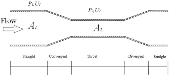
Figure 1. Schematic diagram of Venturi tube structure.

Table 1. Experimental condition points.

P (MPa)	${\mathit{Q}}_{\mathit{g}}$ (m3/h)	${\mathit{Q}}_{\mathit{l}}$ (m3/h)	WLR (%)
0.1, 0.2, 0.3	15, 20, 25, 30,	0.2, 0.3, 0.4, 0.5,	50, 57.1, 60, 62.5, 66.7, 71.4,
	35, 40, 50, 60	0.6, 0.7, 0.8	75, 80, 83.3, 85.7, 87.5

2.1. Physical Constraint Terms of Oil-Gas-Water Three-Phase Flow

The schematic diagram of single-phase flow through a Venturi tube is shown in Figure 1. The upstream cross-sectional area and the throat cross-sectional area are denoted by subscripts 1 and 2, respectively. A represents the cross-sectional area, U is the flow velocity, P is the cross-sectional pressure, and m signifies the mass flow rate. We assume the flow is a stable, one-dimensional single-phase flow, without considering the influence of gravitational potential energy on pressure, and the viscous friction and local energy loss near the throttling element are represented by a dimensionless coefficient $\varphi$. Under these conditions, the one-dimensional momentum equation for single-phase flow [20] can be expressed as Equation (2), where $\varphi$ is a coefficient related to the diameter ratio.

$$(P_1-P_2)A_2+\varphi {\displaystyle \frac{m^2}{\rho A_2}}=m(U_2-U_1),\varphi ={\displaystyle \frac{1}{2}}{(1-{\beta }^2)}^2$$

(2)

$$(P_1-P_2)A_g+\varphi {\displaystyle \frac{m_g^2}{\rho A_2}}{+\mathrm{F}}_{gw}{+\mathrm{F}}_{go}=m_g(U_{g2}-U_{g1})$$

(3)

$$(P_1-P_2)A_{w2}+\varphi {\displaystyle \frac{m_w^2}{\rho A_2}}{+\mathrm{F}}_{wo}-{ \mathrm{F}}_{gw}=m_w(U_{w2}-U_{w1})$$

(4)

$$(P_1-P_2)A_{o2}+\varphi {\displaystyle \frac{m_w^2}{\rho A_2}}-{ \mathrm{F}}_{wo}-{ \mathrm{F}}_{go}=m_o(U_{o2}-U_{o1})$$

(5)

The phase continuity equation is expressed in Equations (6)–(8).

$$m_g={\rho }_g{A}_{g1}{U}_{g1}={\rho }_g{A}_{g2}{U}_{g2}$$

(6)

$$m_w={\rho }_w{A}_{w1}{U}_{w1}={\rho }_w{A}_{w2}{U}_{w2}$$

(7)

$$m_o={\rho }_o{A}_{o1}{U}_{o1}={\rho }_o{A}_{o2}{U}_{o2}$$

(8)

Combining Equations (3)–(8) and rearranging, we obtain Equation (9).

$$(P_1-P_2)A_2={\displaystyle \frac{1-{\beta }^4}{2}}({\displaystyle \frac{m_g^2}{{\rho }_g{A}_{g2}}}+{\displaystyle \frac{m_w^2}{{\rho }_w{A}_{w2}}}+{\displaystyle \frac{m_o^2}{{\rho }_o{A}_{o2}}})$$

(9)

By further transforming Equation (9), we can obtain Equation (10).

$$(P_1-P_2)={\displaystyle \frac{1-{\beta }^4}{2A_2^2}}({\displaystyle \frac{m_g^2{A}_2}{{\rho }_g{A}_{g2}}}+{\displaystyle \frac{m_w^2{A}_2}{{\rho }_w{A}_{w2}}}+{\displaystyle \frac{m_o^2{A}_2}{{\rho }_o{A}_{o2}}})$$

(10)

In Equation (10), there is ${\displaystyle \frac{A_2}{A_{g2}}}={\displaystyle \frac{1}{{\alpha }_g}}$ ${\displaystyle \frac{A_2}{A_{w2}}}={\displaystyle \frac{1}{{\alpha }_w}}$ ${\displaystyle \frac{A_2}{A_{o2}}}={\displaystyle \frac{1}{{\alpha }_o}}$. ${\alpha }_g,{\alpha }_w,{\alpha }_o$ represent the cross-sectional area ratio of the venturi throat; thus, Equation (10) can be derived to obtain Equation (11).

$$(P_1-P_2)={\displaystyle \frac{1-{\beta }^4}{2A_2^2}}({\displaystyle \frac{{\rho }_g{Q}_g^2}{{\alpha }_g}}+{\displaystyle \frac{{\rho }_w{Q}_w^2}{{\alpha }_w}}+{\displaystyle \frac{{\rho }_o{Q}_o^2}{{\alpha }_o}})$$

(11)

To obtain the differential pressure value, it is necessary to determine the cross-sectional holdup of the oil-gas-water three-phase system. The cross-sectional holdup of the water phase can be derived from the microwave voltage amplitude signal. Under high gas–liquid ratio conditions, the oil-water two-phase can be equivalent to the liquid phase. Therefore, the cross-sectional holdup of the gas phase can be calculated using the void fraction model of gas–liquid two-phase flow. The cross-sectional holdup of the oil is equal to one minus the cross-sectional holdups of the other two phases [21,22].

The gas phase cross-sectional holdup model utilizes the improved LM mode [23].

$${\alpha }_g={[1+1.52{({\displaystyle \frac{1-x}{x}})}^{0.35}{({\displaystyle \frac{{\rho }_g}{{\rho }_l}})}^{0.36}{({\displaystyle \frac{{\mu }_l}{{\mu }_g}})}^{0.07}]}^{-1}$$

(12)

where $x$ is the gas mass fraction, ${\rho }_g$ is the gas phase density, ${\rho }_l$ is the liquid phase density (in this context, the mixed density of oil and water), ${\mu }_g$ is the gas phase kinematic viscosity, and ${\mu }_l$ is the liquid phase kinematic viscosity (in this context, the mixed kinematic viscosity of oil and water). Since the water phase cross-sectional fraction ${\alpha }_w$ can be determined from the microwave voltage amplitude signal, the oil cross-sectional fraction is given by ${\alpha }_o=1-{\alpha }_g-{\alpha }_w$. The void fraction model also requires the liquid density and kinematic viscosity, hence

$${\rho }_l={\displaystyle \frac{{\rho }_w{\alpha }_w+{\rho }_w(1-{\alpha }_w-{\alpha }_g)}{1-{\alpha }_g}}$$

(13)

$${\mu }_l={\displaystyle \frac{{\mu }_w{\alpha }_w+{\mu }_o(1-{\alpha }_w-{\alpha }_g)}{1-{\alpha }_g}}$$

(14)

$$x={\displaystyle \frac{{\rho }_g{Q}_g}{{\rho }_g{Q}_g+{\rho }_w{Q}_w+{\rho }_o{Q}_o}}$$

(15)

Therefore, we can conclude that

$${\alpha }_g={[1+1.52{({\displaystyle \frac{{\rho }_w{Q}_w+{\rho }_o{Q}_o}{{\rho }_g{Q}_g}})}^{0.35}{({\displaystyle \frac{{\rho }_g(1-{\alpha }_g)}{{\rho }_o(1-{\alpha }_w-{\alpha }_g)+{\alpha }_w{\rho }_w}})}^{0.36}{({\displaystyle \frac{{\mu }_w{\alpha }_w+{\mu }_o(1-{\alpha }_w-{\alpha }_g)}{{\mu }_g(1-{\alpha }_g)}})}^{0.07}]}^{-1}$$

(16)

Ultimately, the calculated value of differential pressure can be obtained:

$$△P_{cal}=(P_1-P_2)={\displaystyle \frac{1-{\beta }^4}{2A_2^2}}({\displaystyle \frac{{\rho }_g{Q}_g^2}{{\alpha }_g}}+{\displaystyle \frac{{\rho }_w{Q}_w^2}{{\alpha }_g}}+{\displaystyle \frac{{\rho }_o{Q}_o^2}{1-{\alpha }_g-{\alpha }_g}})$$

(17)

By combining the calculated differential pressure value ${\mathrm{\Delta }P}_{cal}$ and the measured differential pressure value ${\mathrm{\Delta }P}_{mes}$ (${\mathrm{\Delta }P}_{mes}=\mathrm{\Delta }P$), the physical constraint equation can be derived:

$$f=△P_{mes}-{\displaystyle \frac{1-{\beta }^4}{2A_2^2}}({\displaystyle \frac{{\rho }_g{Q}_g^2}{{\alpha }_g}}+{\displaystyle \frac{{\rho }_w{Q}_w^2}{{\alpha }_w}}+{\displaystyle \frac{{\rho }_o{Q}_o^2}{1-{\alpha }_g-{\alpha }_g}})$$

(18)

2.2. PINN Model for Oil-Gas-Water Three-Phase Estimation

This article employs a method that combines a feedforward neural network with a physical constraint model to establish a PINN model. A typical feedforward neural network has one input layer, with the number of nodes equal to the number of features in the dataset, one output layer, with the number of nodes equal to the number of outputs, and one or more hidden layers, using user-defined node counts plus bias terms. The input to a node in the hidden layer or output layer is a function (activation function) of the weighted sum of the outputs of other nodes. The training process of the neural network is to find the weights and biases that best correlate the input features with the outputs.

The schematic diagram of the physics-informed neural network (PINN) is shown in Figure 2. The PINN model consists of three parts: the basic structure of the feedforward neural network, the physical constraint equation, and the pre-network for some parameters of the physical constraint equation. The basic structure of the model includes an input layer with 18 neurons, equal to the number of input features; four hidden layers with 512, 384, 448, and 128 neurons, respectively; and an output layer with 3 neurons, equal to the number of output features. The ReLU function is selected as the activation function. ReLU is one of the most commonly used activation functions, which has the advantages of simple implementation and numerical stability; ReLU is not prone to gradient saturation, which helps to alleviate the problem of gradient disappearance, especially in the multi-layer network structure adopted in this paper, which helps improve the convergence speed and training stability.

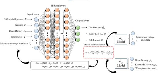
Figure 2. Schematic diagram of PINN (physics-informed neural network).

The PINN model takes differential pressure ($\mathrm{\Delta }P$); pressure ($P$); three-phase density of oil, gas, and water (${\rho }_k(k=g,w,o)$); temperature ($T$); and microwave voltage amplitude ($V_i$) as inputs and infers the volume flow rates of oil, gas, and water ($Q_k(k=g,w,o)$). At the same time, by inputting parameters such as the microwave voltage amplitude ($V_i$), phase density (${\rho }_k(k=g,w,o)$), and kinematic viscosity (${\mu }_k(k=g,w,o)$) into the pre-network, the water phase sectional area fraction (${\alpha }_w$) and gas phase sectional area fraction (${\alpha }_g$) are obtained. Then, the output of the PINN model ($Q_k(k=g,w,o)$) and the water phase sectional area fraction (${\alpha }_w$) and gas phase sectional area fraction (${\alpha }_g$) are input into the physical constraint equation. The physical constraint term f can be calculated and applied to the loss function. The PINN training process is the learning of data and physical terms by optimizing the loss function. Through physical constraints, it can become more physics-informed and prevent overfitting caused by excessive learning of data.

$$Loss={\theta }_{1}MSE\_Q_g+{\theta }_{2}MSE\_Q_w+{\theta }_{3}MSE\_Q_o+{\theta }_{4}REL\_Q_g+{\theta }_{5}REL\_Q_g+{\theta }_{6}REL\_Q_g+{\theta }_{7}MSE\_f$$

(19)

$$MSE\_Q_k={\displaystyle \frac{1}{n}}{\displaystyle \sum _{i=1}^n(\widehat{Q_{k,i}}-Q_{k,i}}{)}^2$$

(20)

$$REL\_Q_k={\displaystyle \frac{1}{n}}{\displaystyle \sum _{i=1}^n\frac{\left|\widehat{Q_{k,i}}-Q_{k,i}\right|}{\left|Q_{k,i}\right|}}$$

(21)

$$MSE\_f={\displaystyle \frac{1}{n}}{{\displaystyle \sum _{i=1}^n(\widehat{f})}}^2$$

(22)

$MSE\_Q_k(k=g,w,o)$ describes the difference between the predicted value and the target value in terms of numerical values, $REL\_Q_k(k=g,w,o)$ describes the relative difference between the predicted value and the target value, while $MSE\_f$ represents the residual of the physical equation, where $n$ is the number of training data.

In order to avoid manually adjusting the weight repeatedly, this study adopts an adaptive balance strategy based on exponential moving average (EMA): the data error items ($MSE\_Q_k$, $REL\_Q_k$) and physical constraint items $MSE\_f$ are exponentially smoothed in each training cycle, and the values of ${\theta }_1-{\theta }_8$ are dynamically updated according to the relative size of the smoothing value so that the data error and physical error are kept in the same order of magnitude during the training process, avoiding a certain kind of loss dominating the optimization process. In this way, a dynamic balance can be achieved between “fitting the experimental number constraint” and “satisfying the physical constraint”.

In the training process, the physical boundary condition is explicitly written into the loss function of the PINN through the residual term f, and its mean square error is recorded as $MSE\_f$, which, together with the mean square error ($MSE\_Q_k$) and relative error ($REL\_Q_k$) term of three-phase volume flow, constitute the total loss. In the training process, we rely on the automatic differentiation mechanism and standard back-propagation algorithm provided by the deep learning framework to directly calculate the gradient of the total loss to all network parameters, rather than using numerical approximation such as finite difference. In this way, the physical boundary and related physical constraints embedded in the PINN are fully reflected in the gradient calculation and parameter optimization process, which helps to ensure the stability of the training process and the physical consistency of the prediction results. The optimization algorithm uses Adam, the epoch is 148, the batch size is 16, the initial learning rate is 1 × 10⁻⁴, and dropout is 0.

The artificial network used in this study aims to achieve smooth and deterministic mapping from the measured signal to the three-phase volume flow, and the physical residual is also calculated directly based on the network output. If non-zero dropout is introduced into the hidden layer, some neurons will be randomly inactivated during forward propagation, and additional random noise will be introduced into the intermediate feature representation and physical residual term, which will weaken the accuracy of physical constraints and may reduce the convergence speed and final prediction accuracy. Based on the above considerations, the dropout ratio is set to 0 in this paper.

Figure 3 shows the convergence curve of loss with epoch in the process of PINN training. It can be seen that the loss decreases monotonically and tends to be stable in a limited number of rounds, indicating that the selected network structure, loss design, and optimization strategy can achieve stable convergence.

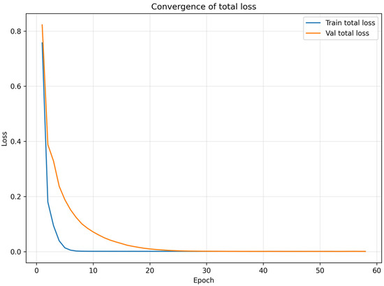
Figure 3. PINN model training convergence curve graph.

2.3. Horizontal Oil-Gas-Water Three-Phase Flow Experiment

2.3.1. Experimental Setup

The horizontal oil-gas-water three-phase flow experiment was conducted in the Multiphase Flow Laboratory of Tianjin University. The experimental setup is shown in Figure 3. The three-phase oil-gas-water is mixed through the inlet pipeline and enters the experimental section. The inner diameter of the experimental pipeline is 50 mm, made of stainless steel, and the experimental medium is air, water, and 3# industrial white oil (the dielectric constant of air is 1, the dielectric constant of tap water is 78, and the dielectric constant of white oil is 2.2). Tap water and industrial white oil are extracted into the pipeline through an industrial peristaltic pump, and the gas phase is provided by an air compressor. The experimental conditions are shown in Table 1, where $Q_g$ is the gas phase flow rate, $Q_l$ is the liquid phase flow rate, and WLR is the liquid phase moisture content. In order to ensure sufficient fluid flow, a 2 m horizontal transition section is set upstream of the sensor. After the sensor measurement is completed, the oil, gas, and water phases enter the gas–liquid separation tank. When the oil and water in the separation tank reach the maximum capacity, the experiment is suspended. After oil-water separation, they are respectively introduced into the water tank and oil tank to continue the experiment. The room temperature in the laboratory is 25 °C, and the humidity is 40%.

The differential pressure transmitter is used to measure the pressure difference between the upstream section of the venturi and the throat, with a range of 0–5 kPa, ±0.1% FS. Pressure and temperature are measured using integrated temperature–pressure sensors, with a temperature range of −10 °C–80 °C and a temperature accuracy of ±2 °C. The pressure range is 0–2 MPa, and the pressure accuracy is ±0.5% FS. The reference flow rates of water and oil phases are measured by a turbine flow meter, with a range of 0–1.2 m³/h and an accuracy of 0.5. The reference flow rate of the gas phase is measured by a turbine flow meter, with a range of 3–140 m³/h and an accuracy of level 1.

2.3.2. Sensor System

The Venturi tube is a common throttling differential pressure flow meter, which has the advantages of simple structure, wide applicability, low pressure loss, and long service life. It is widely used for wet gas measurement under high gas–liquid ratio conditions. When microwaves pass through substances containing polar molecules (such as water), phase delay and amplitude attenuation occur, which is called the polarization phenomenon. The dielectric constant is defined as a quantitative reaction of the properties of the dielectric material, with the dielectric constants of water and air being 80 and 1, respectively. Therefore, the mixed dielectric constant is dominated by the moisture content, which affects the amplitude and phase characteristics of the microwave resonator.

Due to the instability of oil-gas-water three-phase flow under high gas–liquid ratio conditions, if a microwave resonant cavity is connected in series with a Venturi tube, it will result in a difference in the measured water content between the microwave resonant cavity and the Venturi tube. Therefore, this study adopts a dual sensor measurement method of “Venturi tube + microwave resonator” and embeds a microwave resonant cavity at the throat of the Venturi tube, with a resonant cavity distance of about 6d from the contraction section (d is the throat diameter of the Venturi tube). In order to ensure that microwaves can be transmitted through pipelines to obtain information on changes in moisture content, the throat waveguide is made of ceramic with a dielectric constant of 8. When the three-phase flow of oil, gas, and water passes through a Venturi tube, due to the throttling effect, the fluid accelerates and the flow pattern changes. Therefore, pressure signals are collected before the contraction section of the Venturi tube, throat pressure signals, and microwave voltage amplitude signals, and then PINN (physics-informed neural network) is integrated for flow detection of oil, gas, and water three-phase flow. The schematic diagram of the sensor is shown in Figure 4, where the Venturi tube consists of a contraction section throat and an expansion section. MRCS is a microwave-resonant cavity sensor located at the throat of the Venturi tube, and its main structure includes a waveguide and an antenna. For specific structural parameters, refer to the relevant literature [24].

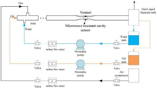
Figure 4. Schematic diagram of oil-gas-water three-phase flow experimental device.

In a circular waveguide, there are TE and TM propagation modes. The TE mode is a transverse electromagnetic wave ($Ez$= 0, $Hz$ ≠ 0), and the TM mode is a transverse magnetic wave ($Ez$ ≠ 0, $Hz$ = 0). In this study, the TM working mode was selected. The specific resonance modes (TM010, TM110, etc.) will be determined based on subsequent dynamic experiments. The calibration experiment of microwave resonant cavity refers to the original static experiment of the research group. The specific operation steps can be found in the static experiment section of Yang’s article [9]. In this article, the measurement accuracy of resonant cavities is as follows, with an accuracy of ±3% in the range of 0–100% and ±1% in the range of 0–10%.

For each operating point, after adjusting the flow rate of each phase to the target value, there was a wait for the system to reach a stable state. Then, the differential pressure ($\mathrm{\Delta }P$), pressure ($P$), temperature ($T$), and microwave voltage amplitude ($V_i$) were continuously recorded at the sampling frequency of fs = 100 Hz for 5 s, and the instantaneous samples of $N$ = 500 of each signal at each working point were obtained. The arithmetic mean of the 5 s data after removing obvious outliers was used as the representative value for this steady-state collection. To further reduce the impact of random fluctuations, each operating point was collected three times under steady-state conditions, and the three representative values were averaged again to yield the final data for that operating point, which were used for subsequent PINN training and evaluation.

3. Results and Discussion

3.1. Analysis of the Coupling Relationship Between Signal and Phase Volume Flow Rate

In the PINN model constructed in this paper, differential pressure ($\mathrm{\Delta }P$) and microwave voltage amplitude ($V_i$) are used as inputs, while the volume flow rates of oil, gas and water ($Q_k(k=g,w,o)$) are regarded as outputs. From the perspective of the coupling between multiphase flow physical mechanisms and data-driven models, the changes in differential pressure and microwave voltage amplitude will cause variations in the predicted values of the volume flow rates of oil, gas, and water. The essence lies in that the alterations in the volume flow rates of oil, gas and water will trigger dynamic evolutions in the phase distribution, dielectric properties, and mechanical responses of the flow field, thereby leading to specific characteristic changes in the differential pressure signal ($\mathrm{\Delta }P$) and microwave voltage amplitude signal ($V_i$). Therefore, by conducting signal analysis on the differential pressure signal and microwave voltage amplitude signal during the experimental process, we confirmed that the changes in the volume flow rates of oil, gas and water ($Q_k(k=g,w,o)$) will cause changes in the differential pressure signal and microwave voltage amplitude signal, and there exists a certain specific pattern. Based on this, through the analysis of the differential pressure signal and microwave voltage amplitude signal during the experimental process, this study systematically confirms the quantifiable coupling relationship and inherent laws between the volume flow rates of oil, gas, and water and the above two types of signals, providing experimental-level support for the physical interpretability and predictive rationality of the “input–output” mapping relationship of the PINN model.

First, to analyze the influence of gas phase flow rate on the differential pressure signal, we conducted comparative experiments. In each experimental group, the liquid phase flow rate was fixed (with liquid phase flow rates of 0 m³/h, 0.2 m³/h, 0.3 m³/h, 0.4 m³/h, 0.5 m³/h, 0.6 m³/h, 0.7 m³/h, and 0.8 m³/h), while the gas phase flow rate was varied to record the values of the differential pressure signal. Figure 5 illustrates the relationship between the gas phase flow rate and differential pressure signal values.

Figure 5. Schematic diagram of sensor structure (Venturi tube + microwave resonator).

In the figure, it can be seen that under the condition of a fixed liquid flow rate, as the gas flow rate increased, the differential pressure also increased accordingly, indicating that the gas flow rate will affect the differential pressure signal, and also demonstrating the rationality of using the differential pressure signal as an input for the PINN model for predicting the gas flow rate.

Continuing to analyze the influence of the liquid phase flow rate on differential pressure signals, we conducted comparative experiments by fixing the gas phase flow rate for each group of experiments (gas phase flow rates of 15 m³/h, 20 m³/h, 25 m³/h, 30 m³/h, 35 m³/h, 40 m³/h, 50 m³/h, and 60 m³/h) and changing the liquid phase flow rate to read the differential pressure signal values. Figure 6 shows the relationship between the liquid phase flow rate and the differential pressure signal value.

Figure 6. Diagram of relationship between gas flow rate and pressure difference signal.

In the figure, it can be seen that under the condition that the gas phase flow rate is fixed, the differential pressure increases correspondingly with the increase in the liquid phase flow rate. This indicates that the gas phase flow rate affects the differential pressure signal and also verifies the validity of using the differential pressure signal as input to the physics-informed neural network (PINN) model for liquid phase flow rate prediction.

Finally, the influence of water holdup on the microwave voltage amplitude was analyzed. Through frequency sweeping, the frequency points where a monotonic relationship exists between the microwave voltage signal and the cross-sectional water holdup were identified. Figure 7 shows the relationship diagram between the microwave voltage amplitude and the cross-sectional water holdup.

Figure 7. Relationship diagram between liquid flow rate and pressure difference signal.

The operating point is that the gas phase flow is 25 m³/h. As can be seen in the figure, in the range of 5735~5830 MHz, with the increase in water content, the amplitude of microwave voltage also increases correspondingly. There is also a corresponding relationship in other microwave frequency ranges, and only this microwave frequency range under this flow point is shown here. Therefore, the cross-section moisture content can be obtained from the microwave voltage amplitude signal, and it is used as input to the PINN model. As shown in Figure 8, a change in the signal will cause a change in the predicted value of water flow.

Figure 8. Diagram of relationship between microwave frequency and microwave voltage signal.

The comprehensive experimental results show that within the working conditions of this paper, the changes of oil, gas, and water volume flow ($Q_k(k=g,w,o)$) will be mapped onto the measurable characteristics of differential pressure signal ($\mathrm{\Delta }P$) and microwave voltage amplitude signal ($V_i$) through the co-evolution of the phase distribution, effective dielectric characteristics, and voltage drop response; there is a stable and estimable coupling relationship between them. This discovery clarifies the mapping mechanism of PINN model from differential pressure ($\mathrm{\Delta }P$) and microwave voltage amplitude ($V_i$) to the volume flow of oil, gas and water; improves the physical interpretability of the model; and provides a mechanistic evidence model integration path of the physical constraint data-driven method of three-phase flow prediction. It can directly guide the subsequent optimization of sensor frequency band selection, feature extraction, and network physical constraints.

3.2. PINN Model Results

By setting PINN, 75% of the dataset is used for the training set, 15% is used for the validation set, 15% is used for the test set, and the random seed is set to 42. We obtained a comparison between predicted and actual values through training, validation, and testing.

Figure 9, Figure 10 and Figure 11 show a comparison of gas, water, and oil phases in the PINN model, where the horizontal axis represents the actual values of each phase, the vertical axis represents the predicted values of each phase, the dashed line indicates the upper and lower limits of the confidence interval of 90%.

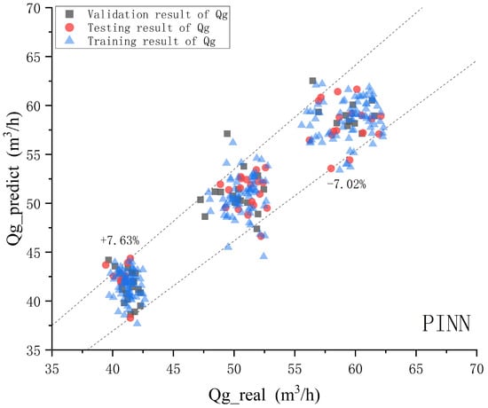
Figure 9. PINN model gas phase prediction effect diagram.

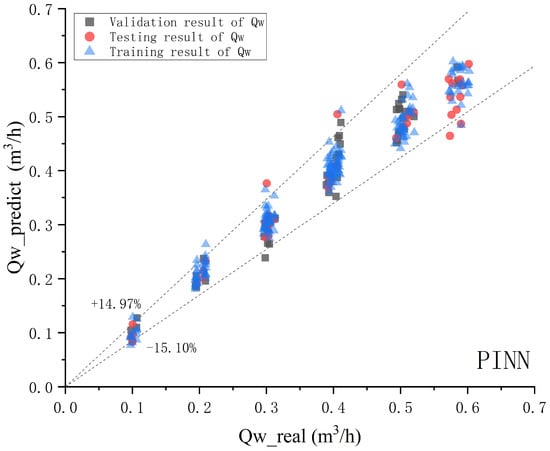
Figure 10. PINN model water phase prediction effect diagram.

Figure 11. PINN model oil phase prediction effect diagram.

According to the comparison chart of the predicted value and the true value of each phase of oil, gas, and water, for the PINN model, with a confidence probability of 90%, the relative error range of the gas phase is −7.02–7.68%. The relative error range of the aqueous phase is −15.1–14.97%. The relative error range of the oil phase is −36.65–31.04%. The correlation coefficients for the gas phase, water phase, and oil phase are 0.941427169, 0.975478243, and 0.848464413, respectively. The PINN model has a good prediction effect.

It should be pointed out that when the gas or liquid flow rate is low, the output signal amplitude of the differential pressure sensor used in this study is close to the lower limit of the range compared to the reference flow meter (standard flow meter), resulting in effective resolution. At this point, even if the absolute deviation caused by small flow fluctuations or noise is small, due to the relative error being calculated with the true value as the denominator, REL will be significantly amplified, resulting in a significantly higher relative error in low-flow areas than in medium- and high-flow areas. In other words, the “relatively large error” in low traffic areas mainly reflects the limitations of measurement resolution and signal-to-noise ratio, rather than the sudden deterioration of model prediction ability in that area. Combined with the absolute error index, it can be seen that even in low-flow areas, the corresponding volume flow deviation is still at a relatively low level (under the experimental range and accuracy conditions in this article), which more objectively reflects the actual deviation level of the model.

In addition to the PINN model, there are other models and machine learning methods applied to flow measurement of oil-gas-water three-phase flow. This section compares artificial neural networks (ANNs) and support vector machines (SVMs) used for regression with the PINN model.

3.3. Comparisons with Other Neural Networks

In order to evaluate the advantages of the PINN model constructed in this paper and ensure that the comparison benchmark is representative, this section selects two typical data-driven methods as reference models: the artificial neural network (ANN) and support vector machine (SVM). The PINN model is based on the ANN model with physical constraints, so it is necessary to compare the PINN model with the ANN model; SVM has good generalization performance and robustness in small sample regression problems and has been widely used in the field of multiphase flow measurement, which can be used as a representative of traditional machine learning methods.

ANN and PINN have exactly the same network structure and training super-parameter settings (including input and output dimensions, number of neurons in each hidden layer, activation function, optimization algorithm, learning rate, batch size, and number of epochs). As a traditional machine learning baseline, a support vector machine (SVM) model is implemented in the form of ε–support vector regression (ε–SVR) with a polynomial kernel. The hyperparameters are tuned on the validation set, and the final model uses a second–order polynomial kernel (kernel = “poly”, degree = 2) with a penalty parameter C = 0.495, ε–insensitive tube width ε = 4.34 × 10⁻³, gamma = “auto”, and coef0 = 0.948. The SVM is trained and tested on exactly the same input features and datasets as the ANN and PINN models, but without any embedded physical constraints, and thus serves as a purely data-driven reference.

Using 75% of the experimental set for training, 15% for validation, and 15% for testing, with a random seed set of 42, we obtained a comparison chart between the predicted and actual values for the two models.

Figure 12, Figure 13 and Figure 14 show a comparison of gas, water, and oil phases in the SVM model, where the horizontal axis represents the actual values of each phase, the vertical axis represents the predicted values of each phase, the dashed line indicates the upper and lower limits of the confidence interval of 90%.

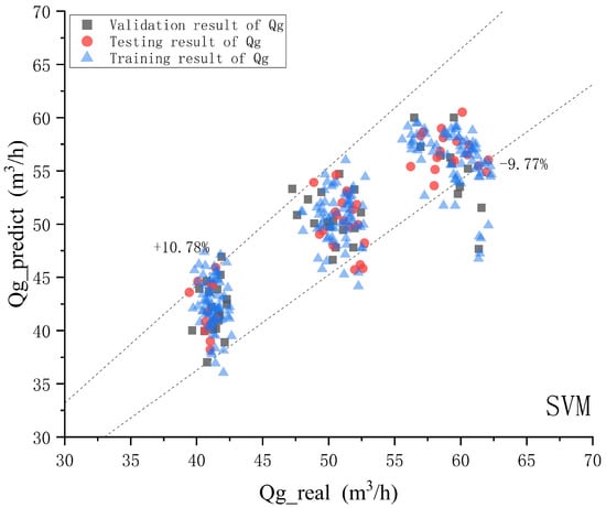
Figure 12. SVM model gas phase prediction effect diagram.

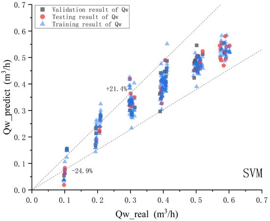
Figure 13. SVM model water phase prediction effect diagram.

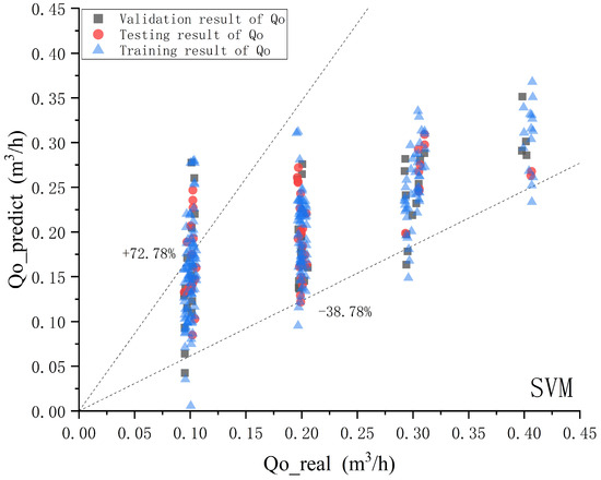
Figure 14. SVM model oil phase prediction effect diagram.

According to the comparison chart between the predicted and actual values for oil, gas, and water phases, for the SVM model, with a confidence probability of 90%, the relative error range for the gas phase is −9.77–10.78%. The relative error range of the aqueous phase is −24.9–21.4%. The relative error range for the oil phase is −32.78–72.78%. The correlation coefficients of gas phase, water phase, and oil phase are 0.90216536, 0.954594502, and 0.652093241, respectively.

Figure 15, Figure 16 and Figure 17 show a comparison of gas, water, and oil phases in the ANN model, where the horizontal axis represents the actual values of each phase, the vertical axis represents the predicted values of each phase, the dashed line indicates the upper and lower limits of the confidence interval of 90%.

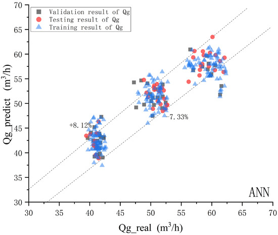
Figure 15. ANN model gas phase prediction effect diagram.

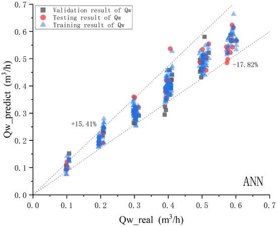
Figure 16. ANN model water phase prediction effect diagram.

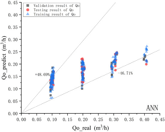
Figure 17. ANN model oil phase prediction effect diagram.

According to the comparison chart of the predicted and actual values of oil, gas, and water phases, for the ANN model, with a confidence probability of 90%, the relative error range of the gas phase is −7.33–8.12%. The relative error range for the aqueous phase is −17.82–15.41%. The relative error range for the oil phase is −46.71–48.69%. The correlation coefficients for gas phase, water phase, and oil phase are 0.932850829, 0.970849258, and 0.743985135, respectively.

Although it can be intuitively and qualitatively observed that the PINN model has a good prediction effect for the comparison diagram of the phase separation predicted value and real value of three different models, this paper calculates the root mean square error (RMSE) and relative error (REL) of oil, gas, and water three-phase volume flow as performance indicators, and quantitatively compares the prediction results. The calculation formulas of RMSE and REL are shown in Formulas (22) and (23), reflecting the deviation between the predicted value ($Q_{pre}$) and the real value ($Q_{rel}$).

$$RMSE=\sqrt{{\displaystyle \frac{1}{n}}{{\displaystyle \sum _{i=1}^n(\widehat{Q_{pre}}-Q_{tr})}}^2}$$

(23)

$$REL={\displaystyle \frac{1}{n}}{\displaystyle \sum _{i=1}^n\frac{\left|\widehat{Q_{pre}}-Q_{tr}\right|}{\left|Q_{tr}\right|}}$$

(24)

The comparison results are shown in Table 2, where the gas-phase flow rate range is 40–60 m³/h. The data in the table are RMSE and REL of the test set. Through the values of various performance indicators in the table, it can be seen that the model of PINN is superior to SVM and ANN, and PINN can accurately predict the split-phase flow of oil, gas, and water under the condition of a high gas–liquid ratio.

Table 2. Comparison Table of RMSE and REL Results for Three Models.

	PINN		ANN		SVM
	RMSE (m3/h)	REL	RMSE (m3/h)	REL	RMSE (m3/h)	REL
$Q_g$	2.1028	0.0397	2.5584	0.0439	3.4588	0.0491
$Q_w$	0.3335	0.0619	0.2888	0.0733	0.0421	0.1289
$Q_o$	0.0435	0.1865	0.0627	0.2713	0.0717	0.3514

As shown in Table 2, in the prediction of gas phase volume flow rate $Q_g$, the PINN model outperforms the ANN model and SVM model in both RMSE and REL indicators (with the minimum RMSE and REL), indicating that introducing physical constraint equations in gas phase measurement can significantly improve prediction accuracy and stability.

For the volume flow rate $Q_w$ of the aqueous phase, the RMSE of each model is of the same order of magnitude. The RMSE of the ANN model is smaller than that of the PINN model and SVM model, but the REL of the PINN model is significantly lower. This is mainly because under the condition of small $Q_w$, the water flow rate itself is small, the microwave signal is close to the detection limit, the signal-to-noise ratio is low, and the absolute error will be amplified after normalization, resulting in a “large variance in the small $Q_w$ region”. In this case, looking at RMSE alone can easily underestimate the relative deviation in low-flow areas, while PINN suppresses overfitting to local noise through physical constraints, making the overall relative error and confidence interval more convergent.

In addition, the overall level of relative error in predicting the volume flow rate of the oil phase is significantly higher than that of the gas phase and water phase. In the low oil phase flow rate region, the PINN model has a smaller absolute error in prediction, but due to the smaller oil phase flow rate reference value, the relative error is further amplified. In the high oil phase flow rate region, the PINN model has relatively small absolute and relative prediction errors. This is the main reason why the error of oil phase prediction is higher than that of the gas phase and the water phase. However, Table 2 shows that the PINN model still has the smallest RMSE and REL in the oil phase, indicating that in the oil phase prediction task with the most unfavorable errors, physics-informed constraints can still significantly reduce the impact of error propagation and accumulation, and the overall prediction performance is better than that of the ANN model and SVM model.

4. Conclusions

This study proposes a new approach to address the safety compliance and engineering feasibility issues associated with online measurement of oil-gas-water three-phase flow under high gas–liquid ratio conditions. A non-radioactive, non-invasive three-phase flow measurement scheme using a “Venturi tube + microwave resonant cavity” and integrating the PINN model is proposed and implemented. A PINN model for predicting the volume flow rate of three-phase oil-gas-water was constructed by embedding physical constraints into the loss function. On a horizontal three-phase flow experimental circuit with a diameter of 50 mm, experimental results show that there is a coupling relationship between differential pressure Δ P, microwave voltage amplitude, and volumetric flow rate of each phase, providing support for the physical interpretability and predictive rationality of the “input-output” mapping relationship of the PINN model.

Compared with ANN and SVM models, the constructed PINN model exhibits better comprehensive accuracy and higher physical consistency in three-phase volume flow prediction. In the test set, the relative errors of PINN for the volumetric flow rates of oil, gas, and water are lower than those of ANN and SVM, and the error distribution is more concentrated, which can satisfy physical constraints while maintaining a similar network size. The above results quantitatively indicate that introducing physics-informed models can substantially improve the accuracy, robustness, and interpretability of three-phase metering models.

It should be emphasized that this study still has certain limitations. Firstly, under high gas–liquid ratio conditions, this study treats the oil-water two-phase system as a single liquid phase and applies an improved LM porosity model to the equivalent gas–liquid two-phase system. The differences in oil-water properties are characterized by effective density and viscosity. The approximation of “simplifying three phases into two phases” does not provide a separate error estimate, and its impact is implicit in the overall prediction error; in working conditions with significant differences in oil-water properties or extreme water content, this approximation may introduce additional deviations. Secondly, the LM model is proposed for gas–liquid systems, and its extension to oil-water systems has certain physical rationality. However, its applicability in more complex flow patterns and a wider range of physical properties still needs to be specifically evaluated and improved.

From the perspective of engineering applicability, the current model has only been trained and validated under laboratory conditions: the pipe diameter is fixed at 50 mm, the pressure range is 0.1–0.3 MPa, the working medium is tap water and white oil, and the temperature and flow pattern range are relatively limited. Therefore, directly extrapolating to field conditions with different pipe diameters, higher or lower pressures, wider temperature ranges, high salinity, and complex flow patterns does not yield strict guarantees. Especially, changes in pressure and temperature can simultaneously affect the compressibility of the gas phase and the dielectric properties of the fluid, thereby altering the mapping relationship between “differential pressure microwave voltage amplitude flow rate”; The salinity of the aqueous phase also has a significant impact on the microwave resonance response, but this study has not conducted a systematic quantitative analysis of it, nor has it included salinity as an explicit input variable in the modeling. In future work, specialized research is needed on salinity changes and their impact mechanisms. In addition, the experimental duration used in this study was relatively limited and conducted in a clean laboratory environment, without addressing issues such as scaling, corrosion, and electronic component drift during long-term operation. Therefore, the long-term stability [25], drift characteristics, and maintenance cycle of the “Venturi tube + microwave resonant cavity” combined with the PINN model in wellhead or field environments still need to be verified through durability tests and on-site trial runs, which also constitutes another important limitation of current work. This study has not yet systematically evaluated the sensitivity of input measurement errors (such as differential pressure, microwave voltage, pressure, and temperature measurement errors) to model output propagation. Therefore, future work will further combine different operating conditions (especially low-flow and extremely low-water-content conditions) to carry out system sensitivity and uncertainty analysis in order to improve the reliability evaluation ability of field applications.

In summary, this study verifies the feasibility and advantages of using the “Venturi tube + microwave resonant cavity + PINN model” for online measurement of high gas–liquid ratio three-phase non-radioactive sources under laboratory conditions. However, its applicability is currently mainly limited by testing conditions and parameter ranges and is constrained by assumptions such as “three phase simplified two-phase” and LM model generalization. In the future, it will need to be calibrated, tested, and subjected to long-term operation testing when applied on-site. Future research will focus on expanding GVF, flow patterns, and pressure–temperature salinity ranges, systematically quantifying the errors introduced by the “simplified three-phase two-phase” and LM-related models under different physical property conditions, and developing porosity/water content correlations more suitable for three-phase flow. Future work will also introduce new sensors to obtain the true cross-sectional gas content, explicitly introducing dielectric parameters such as salinity into PINN for sensitivity and uncertainty analysis. It will also be necessary to conduct long-term operation and calibration tests under wellhead and on-site conditions to evaluate the long-term stability and maintainability of sensors and PINN models, providing a more solid foundation for the engineering application of non-radioactive three-phase flow meters, and conduct system sensitivity and uncertainty analysis to enhance on-site application reliability assessment capabilities. At the same time, we will explore the introduction of modern physics deep learning methods or frameworks and combine them with physical constraints to further enhance the transferability and robustness of the model under a wider range of operating conditions and field conditions.

References

- Rajan, V.S.V.; Ridley, R.K.; Rafa, K.G. Multiphase flow measurement techniques—A review. J. Energy Resour. Technol. 1993, 115, 151–161. [Google Scholar] [CrossRef]
- Shi, X.; Tan, C.; Dong, F.; Escudero, J. Flow rate measurement of oil-gas-water wavy flow through a combined electrical and ultrasonic sensor. Chem. Eng. J. 2022, 427, 131982. [Google Scholar] [CrossRef]
- Fouladinia, F.; Alizadeh, S.M.; Gorelkina, E.I.; Hameed Shah, U.; Nazemi, E.; Grimaldo Guerrero, J.W.; Roshani, G.H.; Imran, A. A novel metering system consists of capacitance-based sensor, gamma-ray sensor and ANN for measuring volume fractions of three-phase homogeneous flows. Nondestruct. Test. Eval. 2025, 40, 2161–2187. [Google Scholar] [CrossRef]
- Li, X.-B.; Hao, X.-Y.; Zhang, H.-N.; Zhang, W.; Li, F.-C. Review on multi-parameter simultaneous measurement techniques for multiphase flow—Part A: Velocity and temperature/pressure. Measurement 2023, 223, 113710. [Google Scholar] [CrossRef]
- Monni, G.; Di Salve, M.; Panella, B. Two-phase flow measurements at high void fraction by a Venturi meter. Prog. Nucl. Energy 2014, 77, 167–175. [Google Scholar] [CrossRef]
- Yuan, C.; Xu, Y.; Zhang, T.; Li, J.; Wang, H. Experimental investigation of wet gas over-reading in Venturi. Exp. Therm. Fluid Sci. 2015, 66, 63–71. [Google Scholar] [CrossRef]
- Luo, Y. Application Research of Venturi Tube in Wet Gas Measurement. Master’s Thesis, Tianjin University, Tianjin, China, 2005. [Google Scholar]
- Yuan, C.; Bowler, A.; Davies, J.G.; Hewakandamby, B.; Dimitrakis, G. Optimised mode selection in electromagnetic sensors for real-time, continuous and in-situ monitoring of water cut in multiphase flow systems. Sens. Actuators B Chem. 2019, 298, 126886. [Google Scholar] [CrossRef]
- Yang, Y.G. Research on the Measurement Method of Phase Volume Fraction in Two-Phase Flow Based on Microwave Resonant Cavity Sensor. Ph.D. Thesis, Tianjin University, Tianjin, China, 2022. [Google Scholar]
- Bai, L.; Jin, N.; Liu, D.; Ren, Y.; Wei, J. Measurement of high water holdup in oil-in-water flows using reticular microwave resonant sensor. IEEE Trans. Instrum. Meas. 2022, 71, 8006811. [Google Scholar] [CrossRef]
- Falcone, G.; Hewitt, G.F.; Alimonti, C.; Harrison, B. Multiphase flow metering: Current trends and future developments. J. Pet. Technol. 2002, 54, 77–84. [Google Scholar] [CrossRef]
- Islamirad, S.Z.; Gholipour Peyvandi, R. Precise volume fraction measurement for three-phase flow meter using 137Cs gamma source and one detector. Radiochim. Acta 2020, 108, 159–164. [Google Scholar] [CrossRef]
- Chen, T.-C.; Alizadeh, S.M.; Alanazi, A.K.; Grimaldo Guerrero, J.W.; Abo-Dief, H.M.; Eftekhari-Zadeh, E.; Fouladinia, F. Using ANN and combined capacitive sensors to predict the void fraction for a two-phase homogeneous fluid independent of the liquid phase type. Processes 2023, 11, 940. [Google Scholar] [CrossRef]
- Chen, H.; Dang, Z.; Hugo, R.; Park, S. CNN-based flow pattern identification based on flow-induced vibration characteristics for multiphase flow pipelines. In Proceedings of the ASME 2022 International Pipeline Conference (IPC 2022), Calgary, AB, Canada, 26–30 September 2022; American Society of Mechanical Engineers (ASME): New York, NY, USA, 2022. [Google Scholar]
- Blaney, S. Gamma Radiation Methods for Clamp-On Multiphase Flow Metering. Ph.D. Thesis, Cranfield University, Cranfield, UK, 2008. [Google Scholar]
- Bahrami, B.; Mohsenpour, S.; Noghabi, H.R.S.; Hemmati, N.; Tabzar, A. Estimation of flow rates of individual phases in an oil-gas-water multiphase flow system using neural network approach and pressure signal analysis. Flow Meas. Instrum. 2019, 66, 28–36. [Google Scholar] [CrossRef]
- Liang, H.; Song, C.; Li, Z.; Yang, H. Volume flow rate calculation model of non-full pipe multiphase flow based on ultrasonic sensors. Phys. Fluids 2023, 35, 033316. [Google Scholar] [CrossRef]
- Li, S.; Bai, B. Gas–liquid two-phase flow rates measurement using physics-guided deep learning. Int. J. Multiph. Flow 2023, 162, 104421. [Google Scholar] [CrossRef]
- Bahrami, S.; Alamdari, S.; Farajmashaei, M.; Behbahani, M.; Jamshidi, S.; Bahrami, B. Application of artificial neural network to multiphase flow metering: A review. Flow Meas. Instrum. 2024, 97, 102601. [Google Scholar] [CrossRef]
- Chisholm, D.A. A theoretical basis for the Lockhart–Martinelli correlation for two-phase flow. Int. J. Heat Mass Transf. 1967, 10, 1767–1778. [Google Scholar] [CrossRef]
- Graham, E.; Reader-Harris, M.; Ramsay, N.; Boussouara, T.; Forsyth, C.; Wales, L.; Rooney, C. Impact of Using ISO/TR 11583 for a Venturi Tube in 3-Phase Wet-Gas Conditions. In Proceedings of the 33rd International North Sea Flow Measurement Workshop, Tønsberg, Norway, 20–23 October 2015; pp. 1–16. [Google Scholar]
- Gajan, P.; Decaudin, Q.; Couput, J.-P. Analysis of High Pressure Tests on Wet Gas Flow Metering with a Venturi Meter. In Proceedings of the 16th International Flow Measurement Conference (FLOMEKO 2013), Paris, France, 24–26 September 2013; pp. 1–8. [Google Scholar]
- Chang, Y.; Xu, Q.; Zou, S.; Zhao, X.; Wu, Q.; Wang, Y.; Thévenin, D.; Guo, L. An improved void fraction prediction model for gas–liquid two-phase flows in pipeline–riser systems. Chem. Eng. Sci. 2023, 278, 118919. [Google Scholar] [CrossRef]
- Xu, Y.; Zuo, R.; Yuan, C.; Fang, L.; Chen, X.; Ma, H. Research on the measurement method of gas-water two-phase flow based on dual-sensor system. Flow Meas. Instrum. 2023, 93, 102393. [Google Scholar] [CrossRef]
- Kamal, B.; Abbasi, Z.; Hassanzadeh, H. Water-Cut Measurement Techniques in Oil Production and Processing—A Review. Energies 2023, 16, 6410. [Google Scholar] [CrossRef]
Disclaimer/Publisher’s Note: The statements, opinions and data contained in all publications are solely those of the individual author(s) and contributor(s) and not of MDPI and/or the editor(s). MDPI and/or the editor(s) disclaim responsibility for any injury to people or property resulting from any ideas, methods, instructions or products referred to in the content. |
© 2026 by the authors. Licensee MDPI, Basel, Switzerland. This article is an open access article distributed under the terms and conditions of the Creative Commons Attribution (CC BY) license.