Improved PPG Peak Detection Using a Hybrid DWT-CNN-LSTM Architecture with a Temporal Attention Mechanism

Abstract

This study proposes an enhanced deep learning framework for accurate detection of P-peaks in noisy photoplethysmographic (PPG) signals, utilizing a hybrid architecture that integrates wavelet-based analysis with neural network components. The P-peak detection task is formulated as a binary classification problem, where the model learns to identify the presence of a peak at each time step within fixed-length input windows. A temporal attention mechanism is incorporated to dynamically focus on the most informative regions of the signal, improving both localization and robustness. The proposed architecture combines Discrete Wavelet Transform (DWT) for multiscale signal decomposition, Convolutional Neural Networks (CNNs) for morphological feature extraction, and Long Short-Term Memory (LSTM) networks for capturing temporal dependencies. A temporal attention layer is introduced after the recurrent layers to enhance focus on time steps with the highest predictive value. An evaluation was conducted on 30 model variants, exploring different combinations of input types, decomposition levels, and activation functions. The best-performing model—Type30, which includes DWT (3 levels), CNN, LSTM, and attention—achieves an accuracy of 0.918, precision of 0.932, recall of 0.957, and F1-score of 0.923. The findings demonstrate that attention-enhanced hybrid architectures are particularly effective in handling signal variability and noise, making them highly suitable for real-world applications in wearable PPG monitoring, digital twins for Heart Rate Variability (HRV), and intelligent health systems.

1. Introduction

Over the past decade, cardiac signal analysis has become a major research area in the field of noninvasive health monitoring. The development of biotechnology and the miniaturization of sensors have led to the increasing use of wearable health devices and have created a need to improve the reliability of PPG (Photoplethysmographic signal) peak detection, as it underlies many physiological measurements. Photoplethysmography is a noninvasive and widely used technology for monitoring heart rate, heart rate variability, and oxygen saturation (SpO₂). Due to its low cost and ease of application, PPG has now established itself as a key technology in wearable and mobile health devices. However, reliable detection of peaks in PPG signals remains a challenge, especially in the presence of noise [1,2]. The nature of the biophysical mechanisms of PPG signal generation is such that this signal is highly sensitive to motion artifacts, baseline drift, and physiological noise [3].

Primary PPG waves are the main pulse waves that are generated by each cardiac contraction and are reflected in the changes in blood volume in the peripheral vessels. They correspond to a PPG signal reflecting cardiac activity and heart rhythm. The systolic wave is the main wave, with high amplitude, that reflects the direct blood flow to the peripheral vessels after the contraction of the left ventricle (systole of the heart). The diastolic (reflected) wave is smaller in amplitude, caused by reflected waves from the peripheral arteries. In a PPG signal, the P-peak (or systolic peak) corresponds to the moment of maximum arterial blood volume in each cardiac cycle. It is physiologically related to the R-peak of the ECG and marks the beginning of the systolic phase, when the left ventricle ejects blood into the arteries. It occurs slightly later in time than the R-peak of the ECG, due to the delay in impulse transit between electrical activation of the heart and the arrival of the pressure wave at the peripheral measurement site. Accurate detection of this peak is crucial for the assessment of heart rate parameters, pulse transit time, and heart rate variability.

Classical approaches to peak detection often rely on adaptive thresholds, signal derivatives, and transform methods. For example, [4] proposes a PPG derivative-based detector that provides relatively good performance in low noise conditions, but suffers from severe distortion.

Traditional algorithms based on threshold methods or wavelet transforms often fail in poor signal quality, varying waveforms, or in the presence of noise [1]. With the development of artificial intelligence and deep learning, new opportunities for automatic and reliable processing of biomedical signals have emerged. Convolutional neural networks (CNN) have been successfully used to extract local features in PPG signals [5], deep neural networks (DNN) are suitable for classification tasks, and recurrent networks such as Long Short-Term Memory (LSTM) can model the temporal dependencies inherent in physiological processes [6,7,8].

Ref. [5] introduced a dilated CNN trained on synthetic noisy data and demonstrate improved robustness at low SNR (Signal-to-noise ratio). The approach is particularly suitable for wearable applications where motion introduces artifacts. Similarly, Mohammadi [9] combined CNN and BiLSTM with an attention mechanism for blood pressure prediction from PPG—which, although not directly for peak detection, confirms the effectiveness of attention structures in analyzing temporal dependencies in PPG signals.

An extended version of these approaches is proposed in [10], where the U-Net architecture is extended with Temporal Attention for more precise peak segmentation, demonstrating significant improvement in mixed noisy data. Attention-based generative networks can be used to transform PPG into ECG, exploiting the capacity of attention to capture long-term dependencies between different physiological signals [11].

The precise localization of peaks also has a clinical context, as it is a starting point for subsequent analyses and correct diagnosis, with predictions of the future widespread use of wearable PPG devices in cardiology, respiratory diseases, neurology and sports [12]. At the same time, BiGRU, even without CNN, when combined with attention, can successfully model and estimate continuous blood pressure fluctuations based on PPG [13].

The application of AI to PPG processing leads to the need for more precise evaluation of neural architectures—not only in terms of accuracy, but also in terms of noise immunity, computational efficiency, and generalization [14].

Recent studies have shown that despite their good ability to capture temporal dependencies in signals, classical LSTM modules suffer from gradient decay with increasing number of layers [15,16] and limited ability to capture long-term dependencies [17,18], which means that this issue should be addressed when using LSTMs.

In this study, we propose a hybrid neural architecture that combines discrete wavelet transform (DWT) for time-frequency signal decomposition, CNN layers for spatial feature extraction, and LSTM with a temporal self-attention mechanism that dynamically determines the importance of different time steps. Such an architecture aims not only to enhance classification accuracy (Precision, Recall, F1), but also to minimize the temporal error in peak detection—an important indicator for clinical application of the mathematical analysis of the variability of time intervals between adjacent heart beats. Simulated and real PPG data are used to train and validate the model, examining the impact of different loss functions, including binary cross-entropy and a new peak distance error metric (Peak Distance Loss).

2. Materials and Methods

2.1. Datasets

PPG signals were recorded in 26 volunteers (14 men and 12 women) over a two-month period from April to May 2025. Measurements were performed using a Shimmer3 GSR+ device (Shimmer Sensing, Dublin, Ireland) equipped with a built-in PPG module with red and infrared light. The sensor was positioned on the finger of the non-dominant hand, and the signals were recorded at a sampling rate of 256 Hz. The data were stored locally on a microSD card, allowing continuous recording without loss of samples, and were subsequently transferred for offline processing and analysis. Recordings were made for 10 min each, with 8 min taken from each initial recording, after the first 2 min (in order to avoid the beginning of the recordings, which may contain noise from start-up artifacts). All signals were resampled to 125 Hz to ensure compatibility between datasets acquired at different sampling rates. To increase the volume and diversity of the training set, publicly available PPG signals from the BIDMC PPG and Respiration Dataset [19] (part of PhysioNet [20]), containing synchronous PPG and respiratory recordings in adults, were added to these records. The BIDMC PPG and Respiration Dataset (version 1.0.0) consists of 53 recordings from inpatients in the intensive care unit of Beth Israel Deaconess Medical Center (Boston, USA). Of these, 20 recordings were from men (mean age 66.45 ± 16.04), 32 recordings were from women (mean age 63.66 ± 18.95), and one recording was missing gender information. The recordings are sampled at 125 Hz.

To prevent data leakage and ensure proper generalization, the dataset was partitioned using a patientwise approach. Each participant’s PPG records were assigned exclusively to one subset—training, validation, or testing—so that segments from the same individual did not appear in more than one subset. The final partition ratio was approximately 70% for training, 15% for validation, and 15% for testing.

This combination of proprietary and public data provided both a high variability of physiological states and a sufficiently generalizable representativeness for training the peak detection model. All participants provided written informed consent prior to inclusion, and the study was conducted in accordance with the Declaration of Helsinki and approved by the Ethics Committee of Institute of Robotics—BAS (protocol approval code: 9/11 February 2025). The study was voluntary; participants could withdraw and terminate their participation at any time. The recipients participated in the data recording free of charge.

2.2. The Proposed PPG Peak Detection System

A schematic representation of the entire PPG peak detection system, including acquisition, preprocessing, and deep learning-based detection, is shown in Figure 1. The diagram illustrates the complete workflow of the proposed PPG peak detection system, covering signal acquisition, preprocessing, and deep learning-based detection. Real PPG signals are acquired using a Shimmer3 GSR+ device, while synthetic PPG signals are generated to expand the dataset and assess robustness. The raw signals are filtered and optionally DWT is applied to extract detailed coefficients and improve peak detection. The input signals are subsequently processed by a hybrid deep learning model, where CNN layers capture morphological (spatial) features, LSTM devices model temporal dependencies, and an attention mechanism focuses on the most relevant peak information. The system architecture supports both experimental and simulated PPG data.

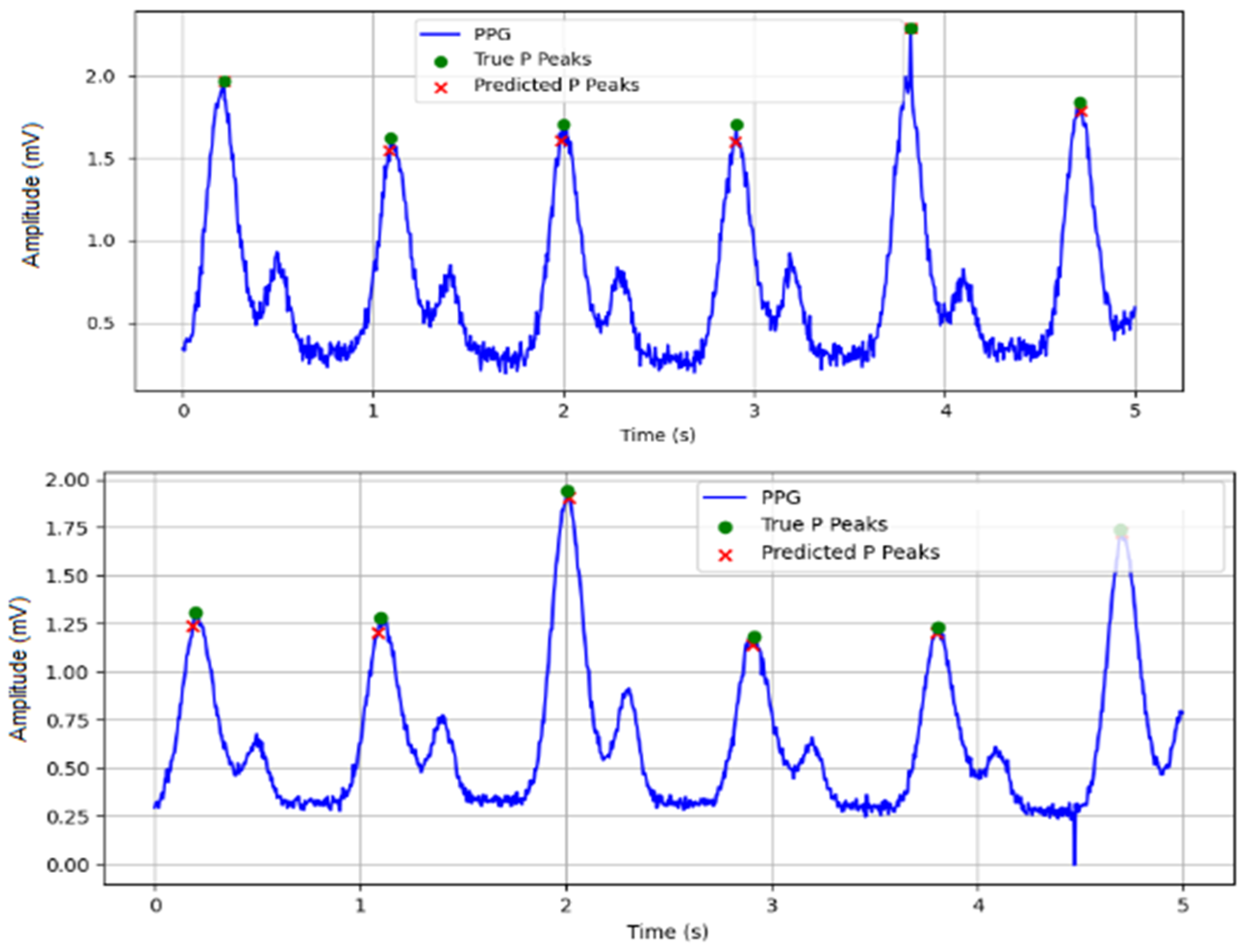
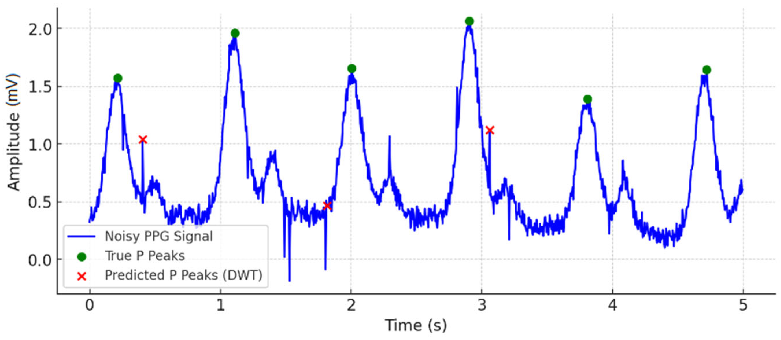
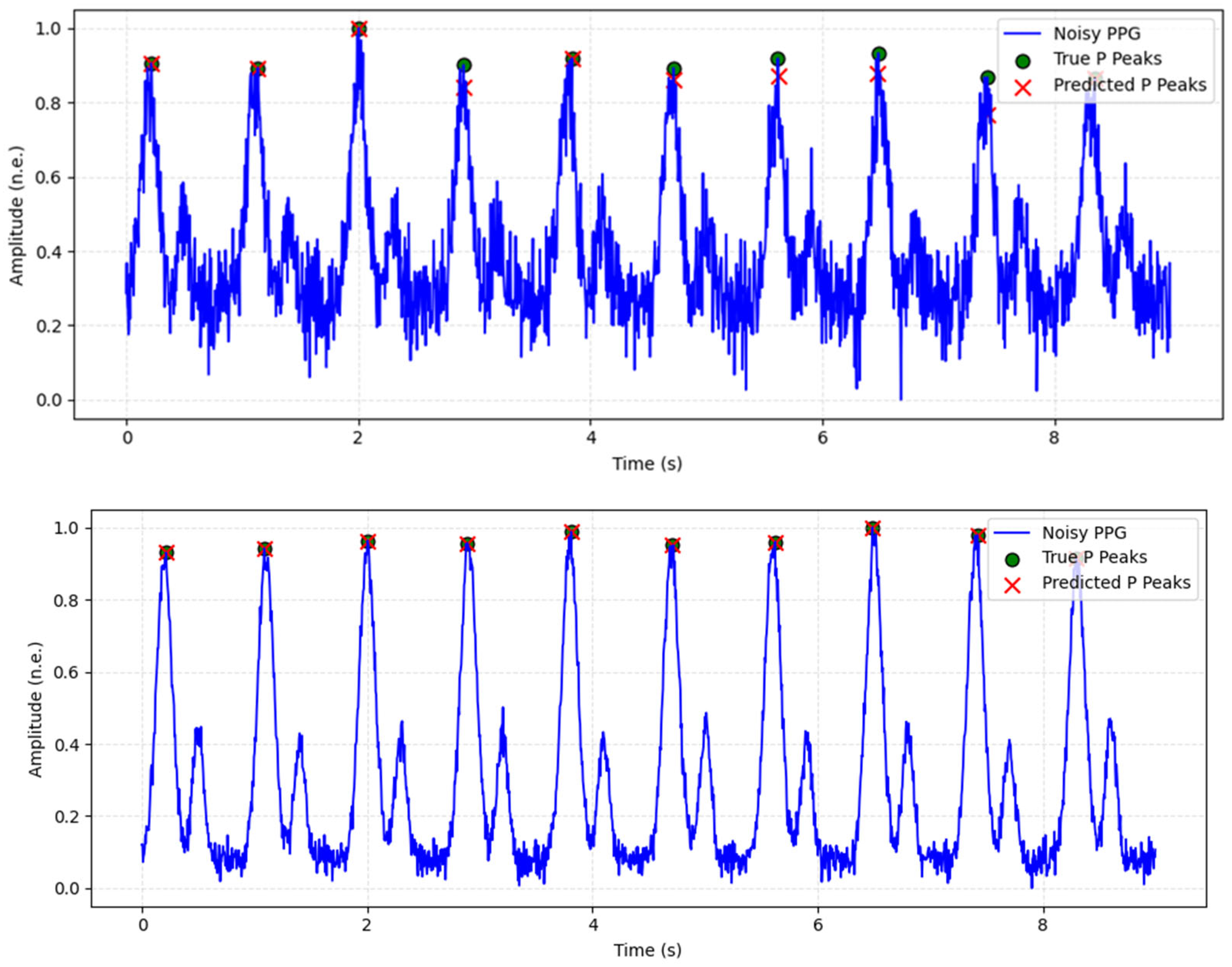
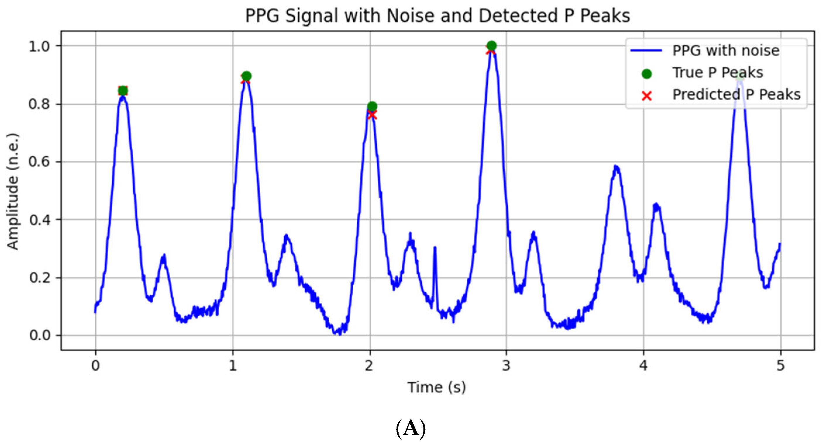
2.3. Description of the Proposed Applied Method

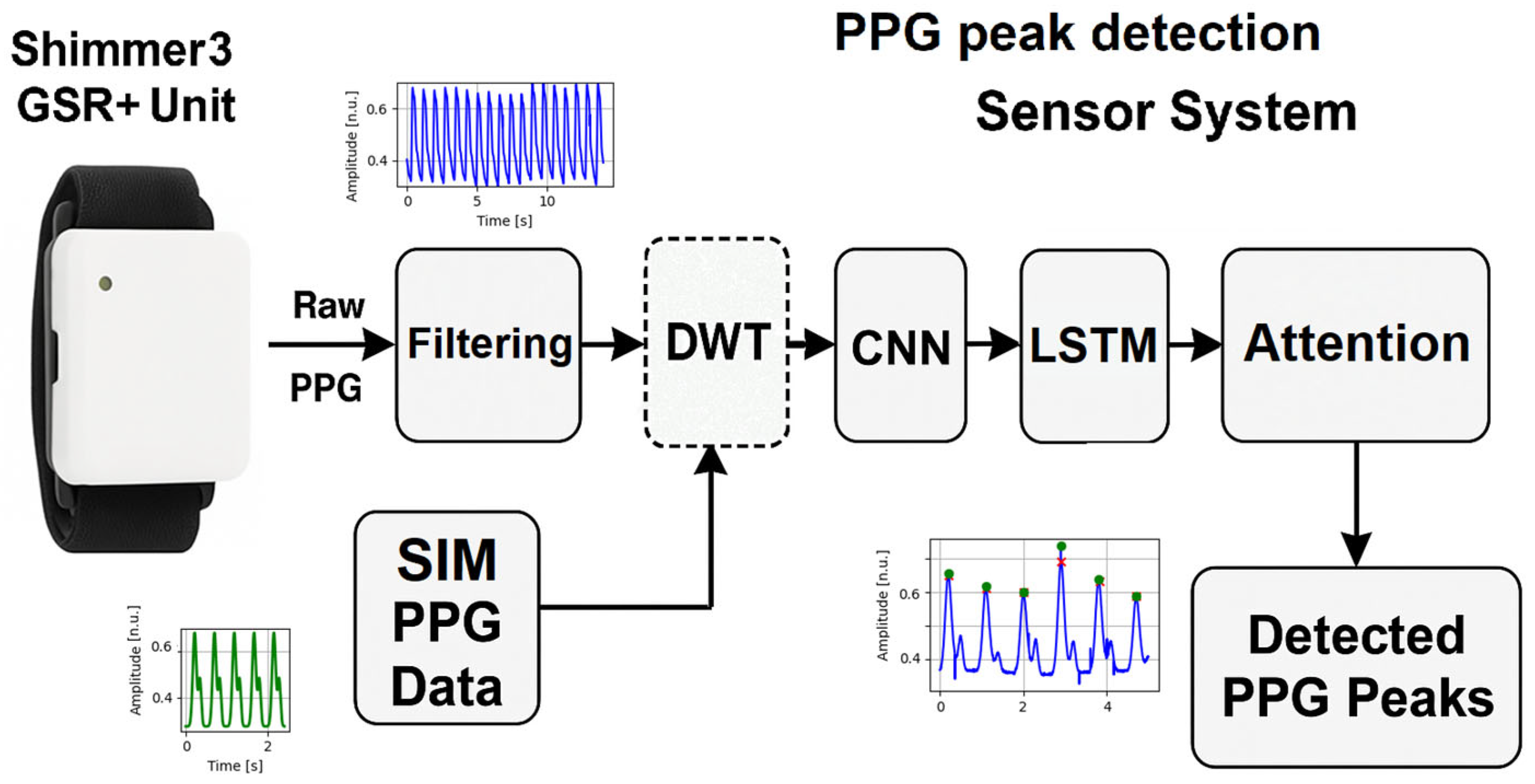
The methodological framework of the proposed approach is summarized in sequential steps to provide a conceptual overview (Figure 2):

• Preprocessing of Raw Data: Butterworth filters are applied, including a high-pass filter with a cutoff frequency of 0.5 Hz to eliminate baseline wander and a band-pass filter with a frequency range of 0.5–10 Hz to isolate the PPG frequency spectrum, remove muscle artifacts, and filter out 50/60 Hz electrical noise. Filtering is performed to prevent incorrect annotations.
• Manual correction of automatically detected P-Peaks: Manual validation of P-peaks is conducted on the training set to ensure maximum objectivity and accuracy.
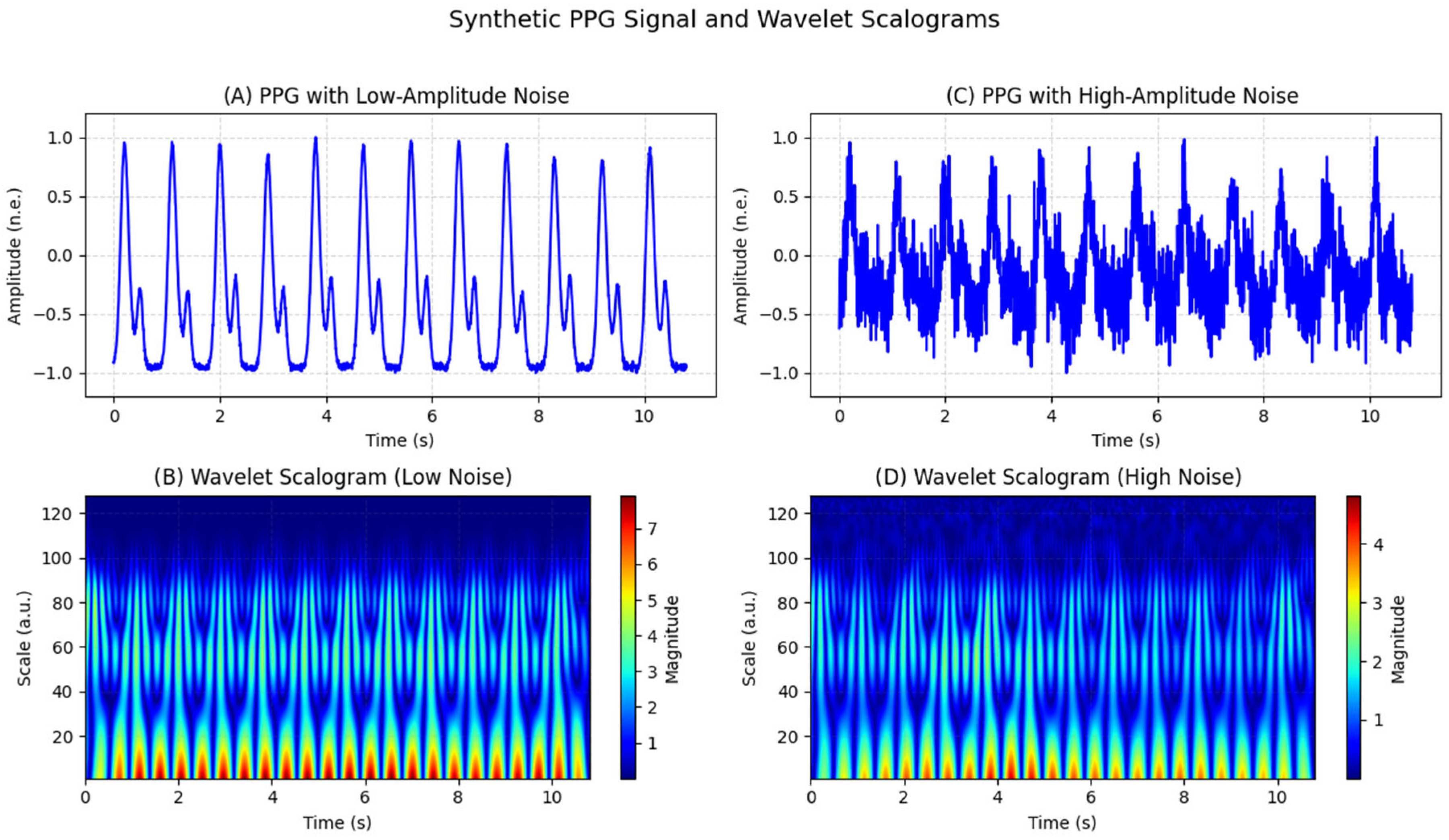
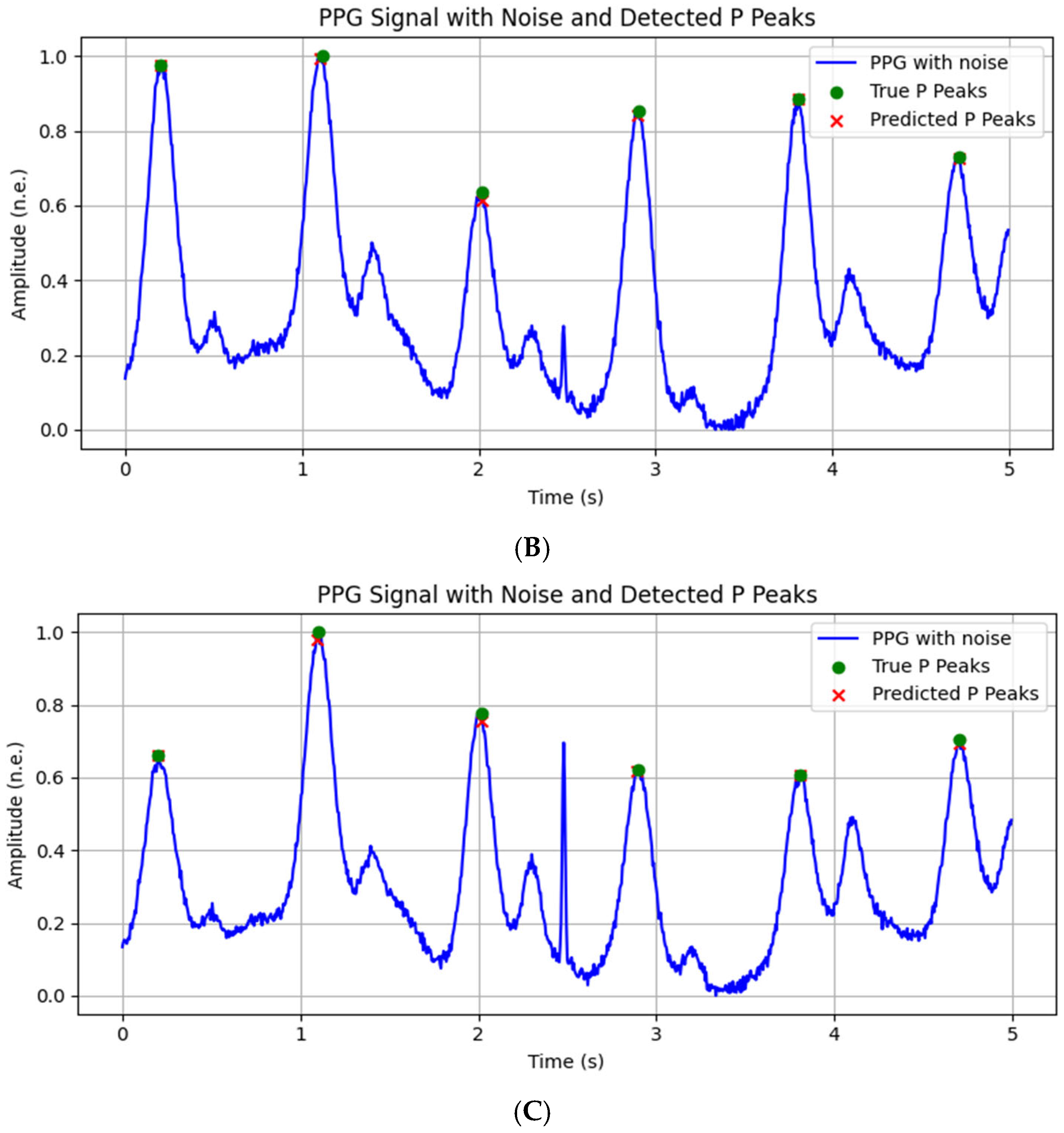
• Noise Augmentation: Noise components such as baseline wander, muscle artifacts, and 50/60 Hz power line interference are added to improve the model’s robustness to real-world conditions.
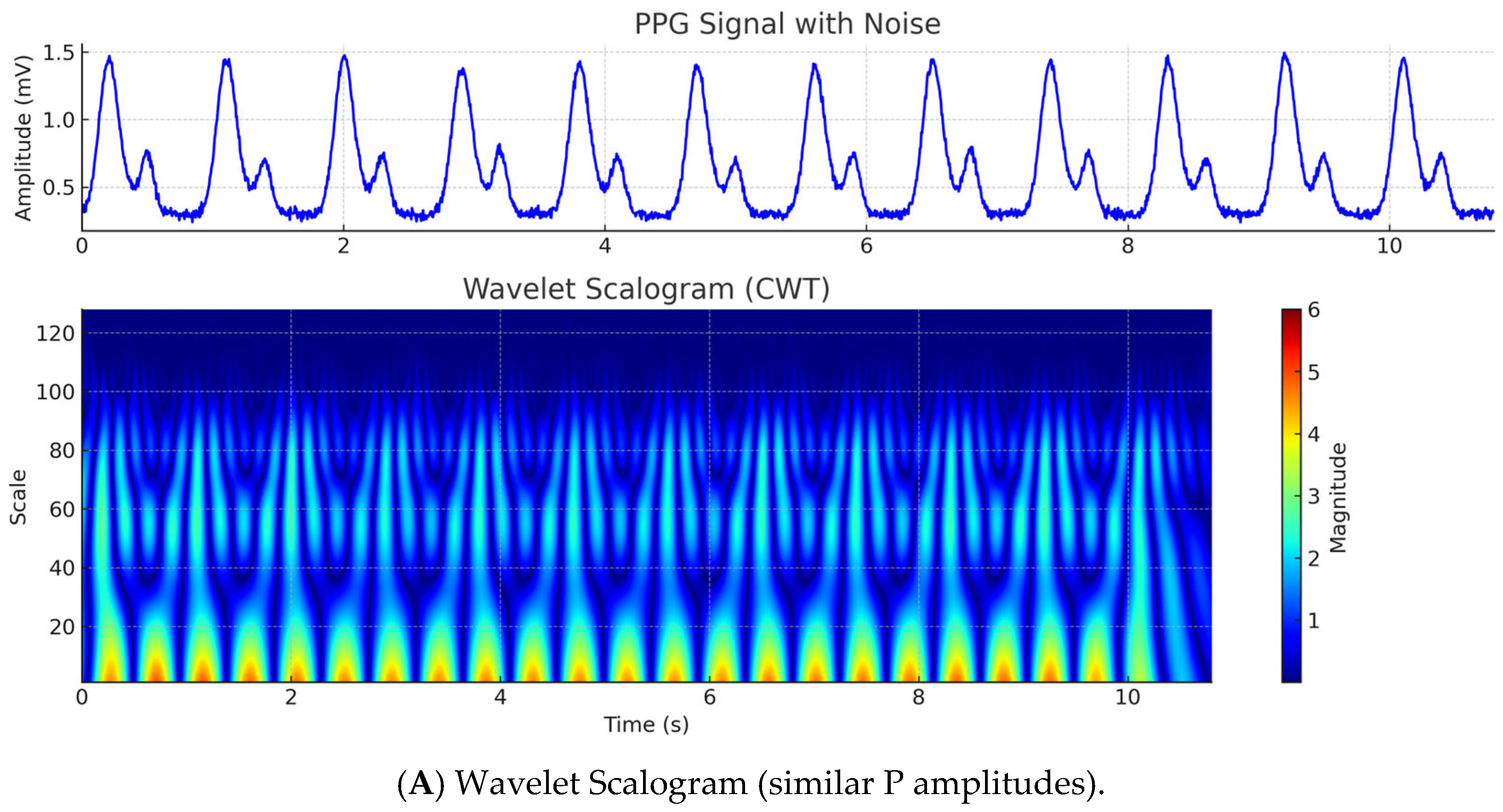
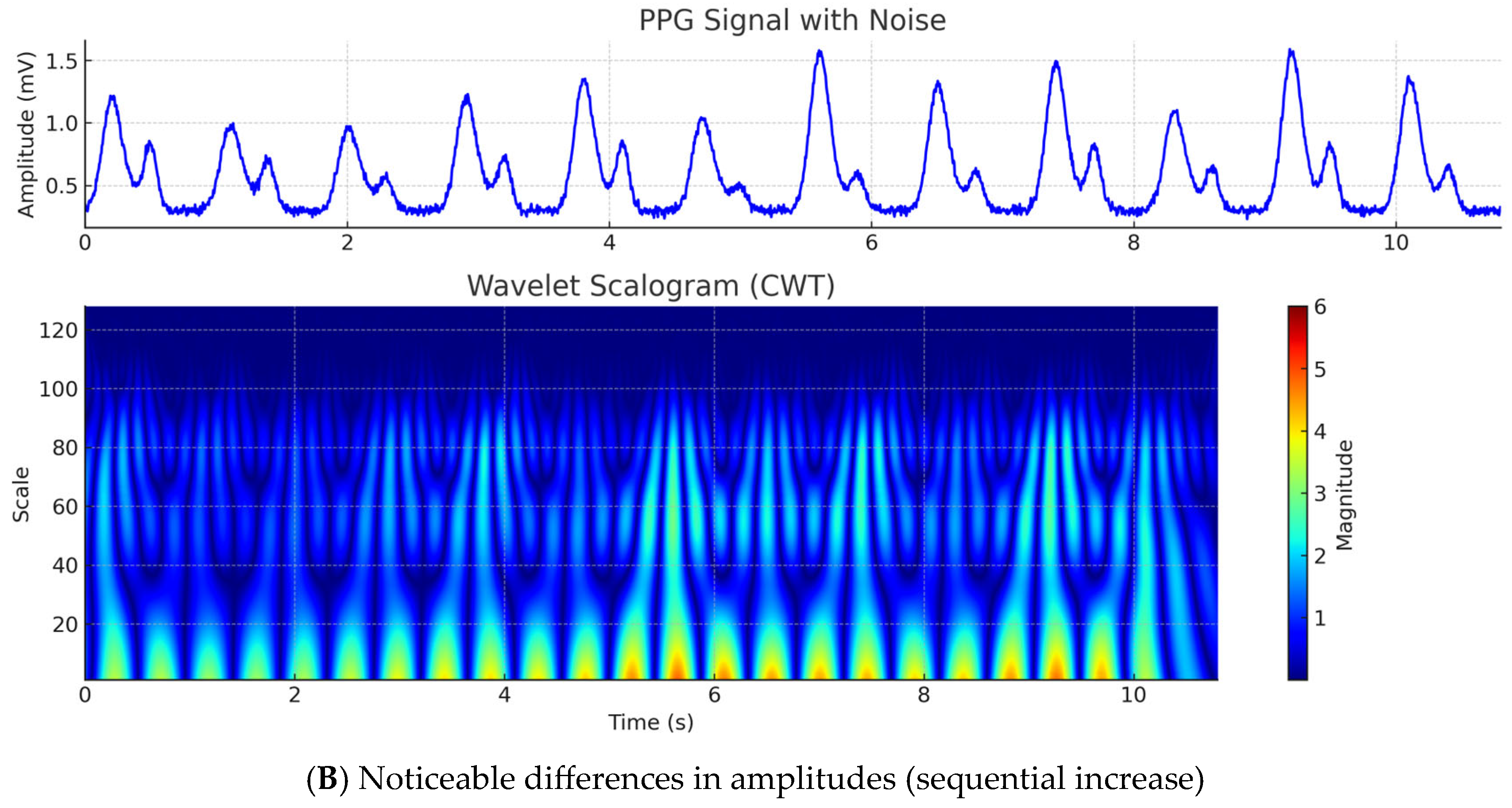
• Application of DWT for Signal Decomposition and Feature Extraction: Wavelet coefficients are extracted using DWT, where detail coefficients from the first to the fourth level are utilized for better localization of P-peaks. In this study, the Daubechies-4 (Db4) wavelet basis was used, with the detailed coefficients being resized to the length of the original PPG segment by linear interpolation, which ensures compatibility along the time axis between channels. These coefficients are used as a second input channel to models that include wavelet decomposition, providing additional time-frequency information about the morphological structure of the P-peak. In models without DWT, only the original PPG signal is used.

DWT with Daubechies wave function with 4 coefficients db4, which is suitable for biomedical signals, with 4 levels of decomposition, is applied. In a previous study by the author, it was experimentally and quantitatively demonstrated that the Db4 wavelet with decomposition level 4 provides optimal performance for PPG peak detection, balancing time–frequency resolution and noise sensitivity [21].

The wavelet coefficients at level j and position k are calculated with the formula

$$W\left(j,k\right)={{\displaystyle \sum }}_{n}x\left(n\right){\phi }_{j,k}\left(n\right),$$

(1)

where

$n$—discrete time index;

$x\left(n\right)$—the input signal;

$j$—decomposition level (scale index);

$k$—translation index;

${\phi }_{j,k}\left(n\right)$—wavelet function (acts as a filter for the corresponding level):

$${\phi }_{j,k}\left(n\right)={\displaystyle \frac{1}{\sqrt{2^j}}} \phi \left({\displaystyle \frac{n-k{2}^j}{2^j}}\right).$$

(2)

5.

Signal Processing with CNN:

5.1.

The signal (in single-channel models this is PPG; in dual-channel models—these are PPG and DWT detail coefficients) is divided into overlapping time windows (2 s with 50% overlap).

5.2.

Conv1D layers are applied to DWT coefficients to extract local features.

5.3.

A MaxPooling layer is incorporated to reduce dimensionality while preserving the most relevant features.

Signal Processing with CNN.

ReLU activation is applied to Convolutional layers:

(x) = max(0,x).

(3)

Equation for the output signal:

$$y_1\left(t\right)=ReLU\left({{\displaystyle \sum }}_{i=0}^{K-1}{x}_{dwt}\left(t+i\right).w_1\left(i\right)+b_1\right),$$

(4)

where

$x_{dwt}\left(t\right)$—input sequence to the CNN layer, which comes from the detailed DWT coefficients at time t;

$w_1\left(i\right)$—convolutional layer filter (of size K).

$b_1$—the bias term of the layer.

The included MaxPooling layer is with Pool Size = 2, formula for the output signal:

$$z_1\left(t\right)=max\left\{y_1\left(t\right),y_1\left(t+1\right),\dots ,y_1\left(t+P-1\right)\right\},$$

(5)

$y_1\left(t\right)$—the input signal from the previous Conv1D layer;

$P$—pool size (MaxPooling layer window size).

A Dropout layer (0.25) has been added after the CNN to combat overfitting. At each iteration, 25% of the neurons in this layer will be randomly dropped, resulting in greater randomness and a more robust model.

The use of 2 s windows with 50% overlap can be interpreted as a form of temporal decomposition, akin to patch-based encoding in recent Transformer models. This strategy allows the model to capture both local waveform features and broader temporal dependencies between adjacent windows. Each window encapsulates a temporally coherent segment of the PPG signal, enabling the CNN layers to focus on high-resolution local features, as the subsequent LSTM and attention layers model the dynamics within the windows. For signal segments at the beginning and end of the recording that do not fully fit into a window, zero-padding is applied to maintain uniform input shape. The overlapping design also ensures smooth temporal coverage and robustness to boundary effects, especially near peak transitions.

6.

Incorporation of LSTM Layers: LSTM layers process sequences of extracted features to identify repetitive patterns in the PPG signal.

Forget Gate is described by the formula

$$f_t=\sigma \left(W_f{x}_t+U_f{h}_{t-1}+b_f\right),$$

(6)

where

$W_f$—Input weight matrix $x_t;$

$x_t$—Input vector for the current moment t;

$U_f$—Weight matrix for the previous hidden state $h_{t-1}$;

$h_{t-1}$—The hidden state from the previous moment;

$b_f$—The Bias vector (added to compensate for the values);

$\sigma$—Sigmoid function that limits the output between 0 and 1.

Input Gate is described by the formula:

$$i_t=\sigma \left(W_i{x}_t+U_i{h}_{t-1}+b_i\right),$$

(7)

Candidate for new information:

$$\widetilde{c_t}=tanh\left(W_c{x}_t+U_c{h}_{t-1}+b_c\right),$$

(8)

Memory update:

$$c_t=f_t\odot c_{t-1}+i_t\odot {\tilde{c}}_t,$$

(9)

Output Gate:

$$o_t=\sigma \left(W_o{x}_t+U_o{h}_{t-1}+b_o\right),$$

(10)

Final LSTM output:

$$h_t=o_t\odot tanh\left(c_t\right),$$

(11)

where

$h_t$ is fed to the next layers for detection of P vertices;

$c_{t-1}$—previous cell memory;

$W_{\ast }, U_{\ast },b_{\ast }$—learnable weight and biases;

$\sigma \left(\cdot \right)$—sigmoid activation;

$\odot$—element-wise multiplication.

In binary classification, a single neuron with sigmoid activation is used:

$$y=\sigma \left(W_{dense}h+b_{dense}\right),$$

(12)

$$\sigma \left(x\right)={\displaystyle \frac{1}{1+e^{-x}}}$$

(13)

At $y\ge 0.5$ it is assumed that a localized peak (1) is present.

At $y<0.5$ it is not a peak.

Binary Cross-Entropy (BCE) is used for the loss function, as the output is a probability (0 or 1):

$$L_{BCE}=-{\displaystyle \frac{1}{N}}{{\displaystyle \sum }}_{i=1}^N\left[y_i log\left({\widehat{y}}_i\right)+\left(1-y_i\right)log\left(1-{\widehat{y}}_i\right)\right],$$

(14)

where

N—number of parameters;

$y_i$—true (labeled) value;

${\widehat{y}}_i$—predicted value obtained by the sigmoid function.

LSTM was selected over simpler recurrent units (e.g., GRU) or temporal convolutions due to its ability to retain long-range temporal dependencies, which is critical for distinguishing subtle rhythmic patterns in PPG morphology.

A second Dropout layer (rate = 0.3) is applied after the LSTM output, before the attention mechanism, to further regularize the temporal encoding and reduce overfitting of the recurrent layers.

7.

Temporal Attention Layer

The inclusion of a temporal attention layer allows the model to assign dynamic importance weights to different time steps in the input sequence. This mechanism improves the model’s ability to focus on temporally relevant segments that are more likely to contain P-peaks, while reducing the weight of less informative or noisy regions. Using the self-attention mechanism in Transformer-based architectures [10], this attention strategy allows for improved peak localization by exploiting the different contributions of temporal context in each sliding window. Unlike static filters or convolutional kernels, attention weights are learned adaptively during training, providing a flexible mechanism for modeling temporal importance.

The context vector c is computed from the hidden states $h_t$ of the LSTM using a temporal attention mechanism that assigns a learned importance weight ${\alpha }_t$ to each time step. This allows the model to focus on the most informative temporal regions within each time window, enhancing peak classification accuracy.

The attention mechanism is mathematically defined as follows. First, a raw attention score $e_t$ is computed for each time step t using a feedforward layer with trainable parameters:

$$e_t=v^{T}tanh(W_h{h}_t+b_h)$$

(15)

These scores are then normalized using the softmax function to obtain attention weights:

$${\alpha }_t={\displaystyle \frac{exp\left(e_t\right)}{{{\displaystyle \sum }}_{i=1}^{T}exp\left(e_i\right)}}$$

(16)

The final context vector is calculated as the weighted sum of all hidden states:

$$\mathrm{c}={{\displaystyle \sum }}_{i=1}^T{\alpha }_t\cdot h_t$$

(17)

where

$h_t$—the hidden state vector at time t;

$W_h$, $b_h$ and $v$—trainable parameters of the attention layer;

${\alpha }_t$—represents the normalized attention weight for each time step;

c—the weighted context vector passed to the output classifier.

The context vector is then forwarded to the classification layer for the final peak prediction. This mechanism ensures that attention is concentrated on segments surrounding true peaks, improving the precision of localization and reducing false positives near waveform transitions.

8.

Output Layer and Post-Processing:

8.1.

A Dense layer with Sigmoid activation is used to predict the probability of each sample being a P-peak.

8.2.

Threshold-Based Detection: An optimal adaptive threshold is determined for peak detection.

8.3.

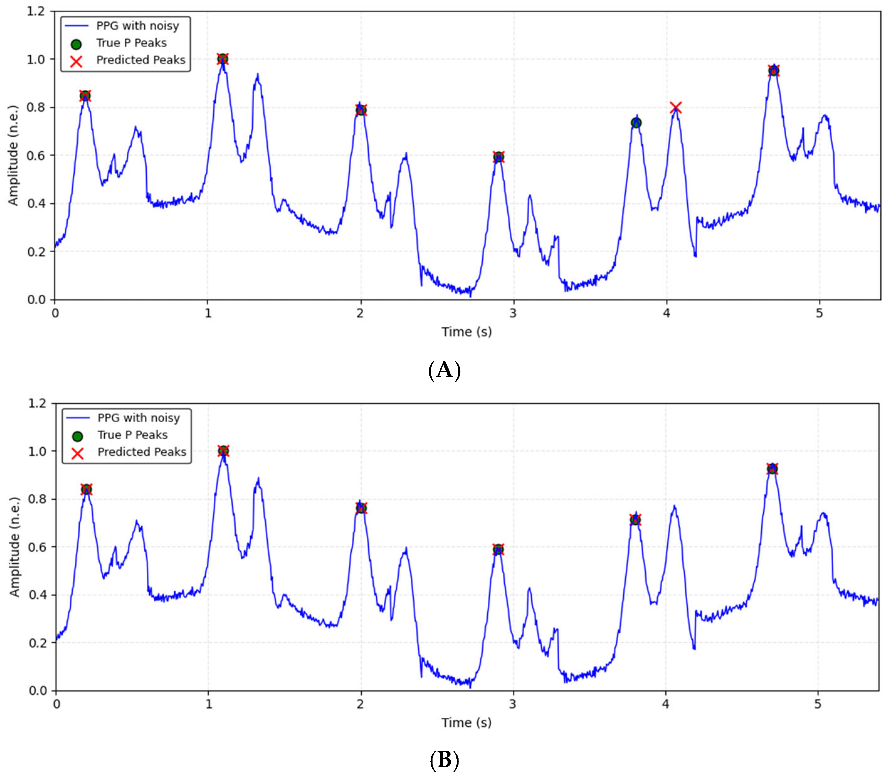
Filtering of Results: Incorrectly detected peaks that do not correspond to local maxima in the signal are removed, and duplicate peaks are eliminated. The peak removal algorithm checks whether each predicted event corresponds to a true local maximum in the filtered PPG signal. If the predicted peak is not a local maximum or falls outside a ±50 ms window of an annotated or valid peak, it is rejected. Potential peak candidates within 200 ms are merged into a set, and the one with the highest amplitude is selected from this set.

9.

Model Training: The dataset is split into 70% for training, 15% for validation, and 15% for testing. The Adam optimizer is used.

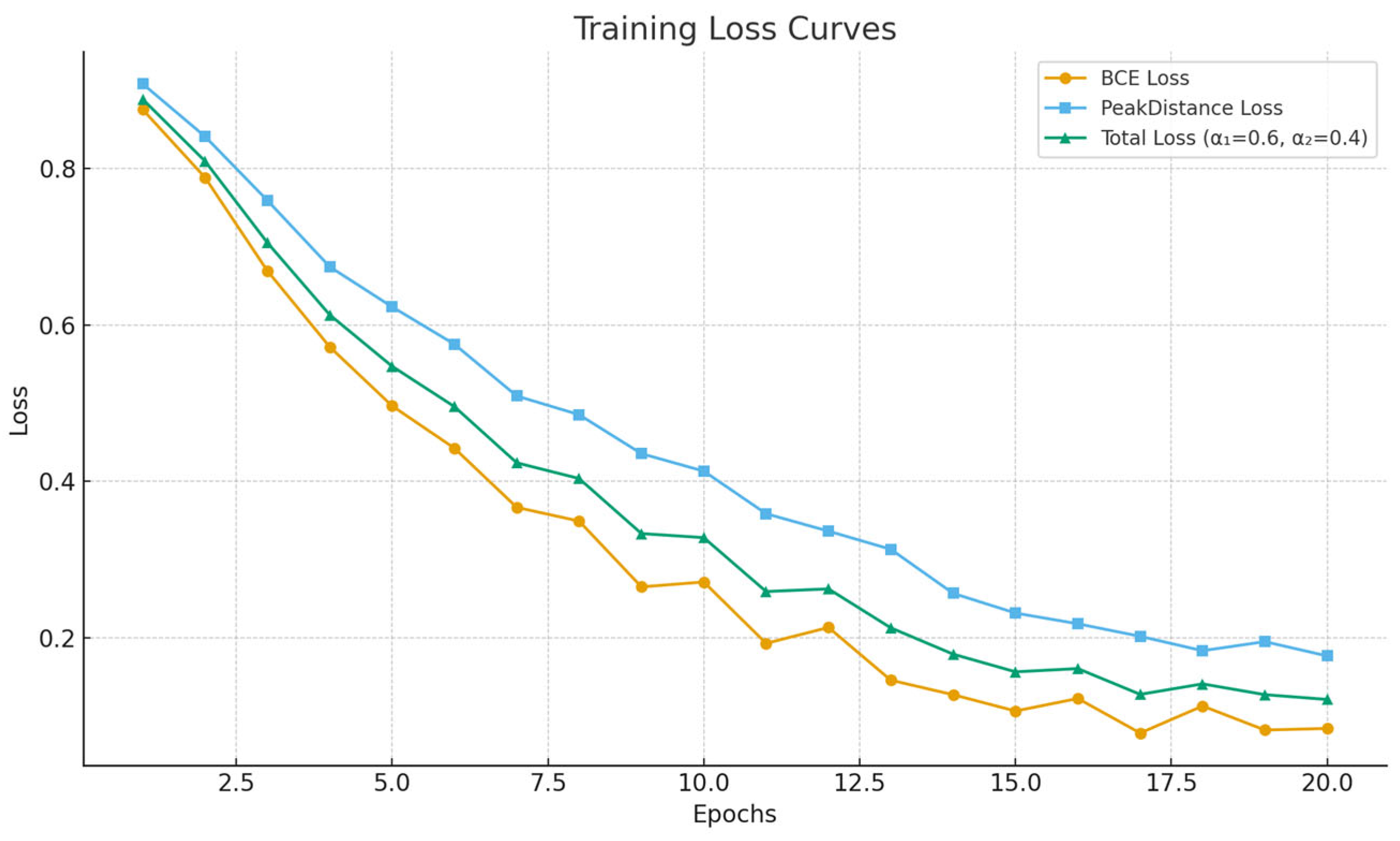
The network is trained using the BCE loss, which is suitable for binary classification tasks such as peak detection (Equation (14)).

To enhance the temporal localization of peaks, we additionally propose a PeakDistanceLoss, which minimizes the distance between true and predicted peaks:

$$L_{DIST}={\displaystyle \frac{1}{N}}{{\displaystyle \sum }}_{i=1}^N\underset{j}{\min }\left|p_i-\widehat{p_j}\right|,$$

(18)

where $p_i$ are the ground truth peak positions, and $\widehat{p_j}$ are the predicted peak positions.

The proposed $L_{DIST}$ (Equation (19)) is formally defined as the average minimal temporal deviation between each reference peak $p_i$ and its nearest predicted counterpart $p_j$. This formulation ensures that the loss is (1) non-negative, with $L_{DIST} = 0$ if and only if all predicted peaks perfectly coincide with the ground-truth positions; (2) monotonically increasing with the temporal displacement $\left|p_i-\widehat{p_j}\right|$, guaranteeing that larger localization errors contribute proportionally higher penalties; and (3) differentiable almost everywhere, allowing gradient-based optimization in end-to-end neural training. Compared to standard amplitude-based losses such as Binary Cross-Entropy or Mean-Squared Error (MSE), which only penalize classification errors at the sample level, $L_{DIST}$ measures temporal accuracy. By minimizing the spatial–temporal misalignment between predicted and true peaks, it provides a direct optimization target for localization tasks.

The total loss combines both terms:

$$L_{TOTAL}={\alpha }_1. L_{BCE}+{\alpha }_2. L_{DIST},$$

(19)

with weighting factors ${\alpha }_1$ and ${\alpha }_2$ used to balance classification and localization performance.

Training data composition and partitioning

To ensure a robust and generalizable model, the dataset was constructed from three complementary sources:

• real PPG recordings from 26 volunteers measured with the Shimmer3 GSR+ device;
• synthetic signals generated by the Deep-SimPPG algorithm [22];
• publicly available data from the BIDMC PPG and Respiration Database [19].

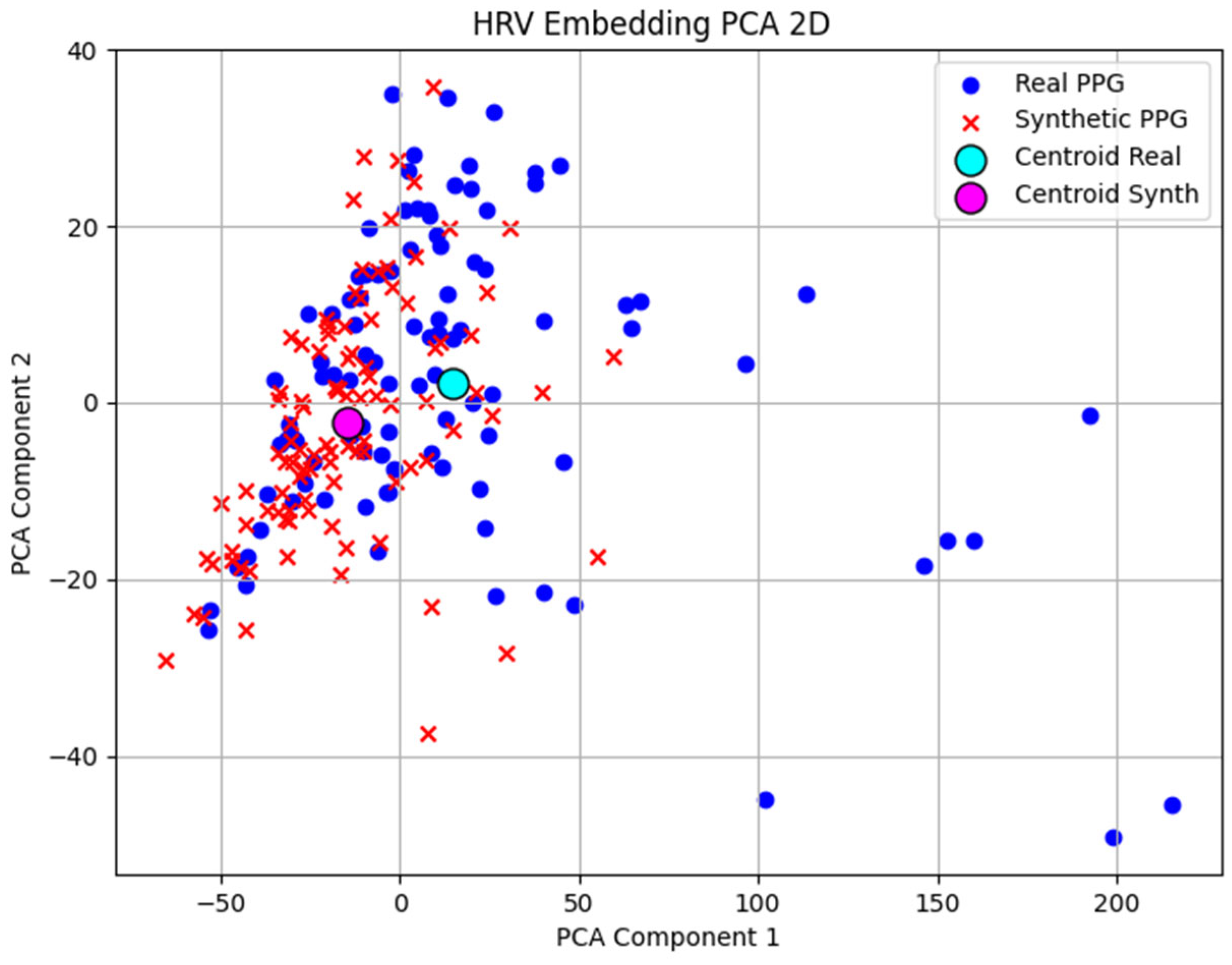
The Deep-SimPPG generator used combines mathematical modeling and generative neural networks implemented with a 1D CNN architecture. In the first stage, a baseline signal is created by summing two Gaussian functions that describe the basic morphology of the PPG pulse wave—the systolic wave, reflecting the direct blood flow from the heart contraction, and the diastolic (reflected) wave, caused by the reflected pulse waves from the peripheral vessels. This baseline signal is fed to the GAN generator, which, by adding noise, enriches its shape with realistic physiological variations and noise artifacts. The discriminator, which is fed both synthetic and real PPG segments, is trained to distinguish real from artificial signals, guiding the generator towards a more realistic synthesized output.

All PPG recordings were segmented into fixed-length 2 s windows with 50% overlap, resulting in a large number of training examples. Only complete segments were used, and zero-padding was applied when necessary. To prevent subject-related data leakage, all segments originating from the same participant or original recording were assigned exclusively to one of the three subsets—training, validation, or testing—ensuring no overlap between them.

Synthetic data were used only in the training and validation phases to improve model robustness to noise and morphological variability. The final testing subset included only unused real recordings from both BIDMC and Shimmer volunteers, ensuring unbiased evaluation of model generalization.

The total data (

Table 1. Composition of the datasets used for model training, validation, and testing.

Purpose	Data Type	Dataset Source	Approx. Segments (2 s.) at 50% Overlapping
Training (136,408 r.)	BIDMC PPG and Respiration Dataset	34 subjects (recordings), 8 min each	16,048
	Shimmer	19 volunteers × 10 recordings (8 min each)	89,680
	Synthetic signals	Deep-SimPPG generator	30,704
Validation (29,240 r.)	BIDMC PPG and Respiration Dataset	7 subjects (recordings), 8 min each	3304
	Shimmer	2 volunteers× 10 recordings (8 min each)	9440
	Synthetic signals	Deep-SimPPG generator	16,496
Testing (29,264 r.)	BIDMC PPG and Respiration Dataset	12 subjects (recordings), 8 min each	5664
	Shimmer	5 volunteers× 10 recordings (8 min each)	23,600

) used is approximately 194,912 two-second recordings, corresponding to approximately 70% training (136,408), 15% validation (29,240), and 15% testing (29,264) (the exact ratio is 69.984%/15.002%/15.01%). Synthetic signals were excluded from the final testing set and to ensure that the model evaluation reflects its application on real PPG data.

A composition of the training, validation, and testing datasets used in the proposed PPG peak detection framework is shown in Table 1. The table summarizes the origin of the data (real, synthetic, or public), their purpose in the training protocol, and the approximate number of 2 s windows (with 50% overlap) used in each subset.

Distribution of records by datasets:

BIDMC PPG and Respiration Dataset: 53 subjects (recordings), 8 min each (25,016 Approx. Segments 2 s. at 50% overlapping).

Shimmer: 26 volunteers × 10 recordings, 8 min each, (122,720 Approx. Segments 2 s. at 50% overlapping).

Synthetic signals: 100 recordings, 8 min each (47,200 Approx. Segments 2 s. at 50% overlapping).

To ensure the robustness of the results and to avoid dependence on a specific random partition, 5-fold cross-validation is applied within the training set: the data is divided into five equal subsets, with one used for validation and the remaining four for training at each iteration. The five results obtained are averaged to provide a statistically reliable estimate of the metrics.

Model Architectures

For analysis and testing of the presented algorithm, a custom Python 3.10 framework was developed to enable the evaluation of multiple model configurations. The models were trained using the Adam optimizer with a fixed learning rate η = 0.001 and 20 epochs. Two commonly used activation functions were explored—Sigmoid and Tanh—to assess their impact on training convergence and prediction accuracy. The architectural configurations of the proposed 30 models are summarized in

Table 2. Types of Models Studied.

Model	Type NM	Input Data Type	Activation Function	Number of Neurons by Level
Type1	CNN	PPG	Sigmoid	16/32/16
Type2	CNN	DWT, 2 level	Sigmoid	16/32/16
Type3	CNN	DWT, 3 level	Sigmoid	16/32/16
Type4	CNN	PPG	Tanh	16/32/16
Type5	CNN	DWT, 2 level	Tanh	16/32/16
Type6	CNN	DWT, 3 level	Tanh	16/32/16
Type7	LSTM	PPG	Sigmoid	16/32/16
Type8	LSTM	DWT, 2 level	Sigmoid	16/32/16
Type9	LSTM	DWT, 3 level	Sigmoid	16/32/16
Type10	LSTM	PPG	Tanh	16/32/16
Type11	LSTM	DWT, 2 level	Tanh	16/32/16
Type12	LSTM	DWT, 3 level	Tanh	16/32/16
Type13	CNN + LSTM	PPG	Sigmoid	16/32/16
Type14	CNN + LSTM	DWT, 2 level	Sigmoid	16/32/16
Type15	CNN + LSTM	DWT, 3 level	Sigmoid	16/32/16
Type16	CNN + LSTM	PPG	Tanh	16/32/16
Type17	CNN + LSTM	DWT, 2 level	Tanh	16/32/16
Type18	CNN + LSTM	DWT, 3 level	Tanh	16/32/16
Type19	CNN + LSTM	PPG	Sigmoid	32/64/32
Type20	CNN + LSTM	DWT, 2 level	Sigmoid	32/64/32
Type21	CNN + LSTM	DWT, 3 level	Sigmoid	32/64/32
Type22	CNN + LSTM	PPG	Tanh	32/64/32
Type23	CNN + LSTM	DWT, 2 level	Tanh	32/64/32
Type24	CNN + LSTM	DWT, 3 level	Tanh	32/64/32
Type25	CNN + LSTM + Attention	PPG	Sigmoid	32/64/32
Type26	CNN + LSTM + Attention	DWT, 2 level	Sigmoid	32/64/32
Type27	CNN + LSTM + Attention	DWT, 3 level	Sigmoid	32/64/32
Type28	CNN + LSTM + Attention	PPG	Tanh	32/64/32
Type29	CNN + LSTM + Attention	DWT, 2 level	Tanh	32/64/32
Type30	CNN + LSTM + Attention	DWT, 3 level	Tanh	32/64/32

, including the type of neural network, input signal transformation, activation functions, and the number of neurons per layer.

The models differ by type of network (CNN, LSTM, CNN + LSTM, and CNN + LSTM + Attention), input data format (raw PPG or DWT-transformed signals at different decomposition levels), activation function, and the number of neurons in the hidden layers (16/32/16 and 32/64/32). The goal was to systematically compare simpler and more complex topologies, as well as the influence of including DWT (detailed coefficients, second or third level) and attention mechanisms, on P-peak detection performance.

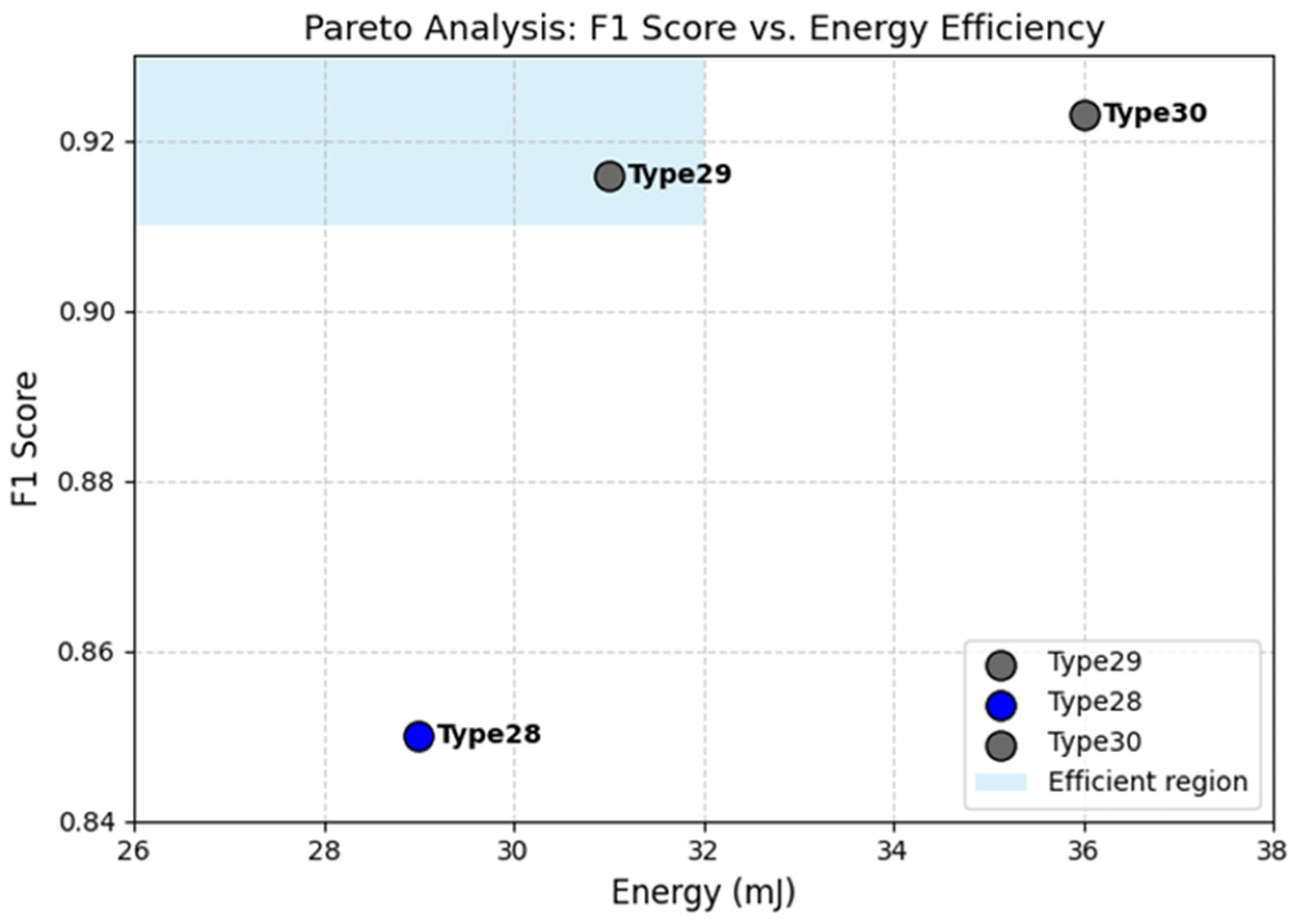
This systematic exploration allowed for identifying the optimal configuration in terms of robustness to noise, computational efficiency, and detection accuracy, as further discussed below.

The number of neurons per layer in each model was determined empirically based on preliminary experiments and architectural symmetry considerations.

Two main configurations were finally evaluated: (16/32/16) for lighter models and (32/64/32) for deeper architectures.

These values were chosen to achieve balanced feature extraction and compression while maintaining an appropriate total number of trainable parameters relative to the size of the available dataset and avoiding overfitting.

The symmetric structure (e.g., 16–32–16) was adopted to allow for progressive feature abstraction in the intermediate layer, followed by dimensionality reduction—similar to encoder–decoder designs.

The larger configurations (e.g., 32–64–32) were used in the CNN + LSTM + Attention models to evaluate the effect of higher representational capacity.

The final number of neurons listed in Table 1 corresponds to the configurations that achieved the highest F1-score on the validation set.

Full Architecture of the Proposed CNN–LSTM–Attention Model

The complete architecture of the model Type30 (

Table 3. CNN–LSTM–Attention Architecture (Type30).

Layer No.	Type	Parameters	Kernel/Units	Activation	Dropout	Output Shape
1	Input	2 s PPG segment with DWT3 detailed coefficients	—	—	—	(250, 2)
2	Conv1D	32 filters	Kernel size = 5	ReLU	0.25	(246, 32)
3	BatchNorm	—	—	—	—	(246, 32)
4	MaxPooling1D	Pool size = 2	—	—	—	(123, 32)
5	Conv1D	64 filters	Kernel size = 5	ReLU	0.25	(119, 64)
6	BatchNorm	—	—	—	—	(119, 64)
7	MaxPooling1D	Pool size = 2	—	—	—	(59, 64)
8	Conv1D	32 filters	Kernel size = 3	ReLU	0.25	(57, 32)
9	BatchNorm	—	—	—	—	(57, 32)
10	LSTM	32 units	—	tanh	0.3	(57, 32)
11	LSTM	64 units	—	tanh	0.3	(57, 64)
12	LSTM	32 units	—	tanh	0.3	(57, 32)
13	Attention Layer	—	Context vector dimension = 32	Softmax (temporal weights)	—	(32)
14	Dense	1 neuron	—	Sigmoid/Tanh	—	(1)

) integrates convolutional, recurrent, and attention layers in a sequential hybrid configuration designed for robust P-peak detection from PPG signals. The model receives as input either a 2 s PPG window with DWT coefficients level 3.

The CNN block extracts local morphological features, while the LSTM block captures temporal dependencies between consecutive waveform patterns. Finally, the attention layer adaptively weights the most informative time steps, emphasizing those likely to contain P-peaks and suppressing noisy regions.

Training Procedure

All models were implemented and trained using Python (TensorFlow environment). The training dataset consisted of annotated PPG signals, preprocessed with optional DWT up to level 3. Each signal window was annotated by marking the time points that fall within the local maximum around the real P-peak (±25 ms). A detected P-peak was considered correct if it occurred within ±25 ms of the reference annotation. The models were trained for 20 epochs using the Adam optimizer with default parameters (learning rate α = 0.001, β₁ = 0.9, β₂ = 0.999). The binary cross-entropy (BCE) loss function was used, as the task was formulated as a binary classification problem (peak vs. no peak). Mini-batch training was employed with a batch size of 64, and early stopping was monitored based on the validation loss with a patience of 5 epochs to prevent overfitting. All signals were normalized to the range [0, 1] before training. Two activation functions were tested: Sigmoid and Tanh. Dropout (rate = 0.2) was applied after each hidden layer to improve generalization. For hybrid models with attention (Type25–Type30), the layer was placed after the LSTM block, before the output dense layer.

Table 4. Training Protocol: Hyperparameters.

Category	Parameter/Setting	Description
Dataset	Total samples	195,000 PPG segments (2 s each, 125 Hz → 250 samples)
	Channels	1–2 (depending on model configuration)
	Split ratio	70% training/15% validation/15% testing
	Preprocessing	Bandpass filter (0.5–8 Hz), normalization (z-score or min–max)
Model architecture	Convolutional layers	3 × Conv1D (32, 64, 32 filters, kernel = 5/5/3, ReLU, Batch Normalization, Dropout = 0.25)
	LSTM layers	3 × LSTM (32, 64, 32 units, Dropout = 0.3)
	Attention mechanism	Temporal attention (Bahdanau-type)
	Output layer	Dense(1, sigmoid) for binary classification
Training configuration	Optimizer	Adam (learning rate = 1 × 10−3, β1 = 0.9, β2 = 0.999)
	Loss function	Binary cross-entropy/ PeakDistanceLoss
	Batch size	64
	Epochs	20 (early stopping, patience = 5)
	Learning rate	0.001
	Regularization	Dropout (0.2–0.3), L2 (=1 × 10−4)
	Initialization	He normal (CNN), Glorot uniform (LSTM)
Hardware and environment	GPU	NVIDIA GeForce RTX 5070 (16 GB VRAM)
	CPU/RAM	3.9 GHz, 64 GB RAM
	Framework	TensorFlow 2.17 (Keras 3.x, Python 3.11)
	Precision mode	Mixed precision (float16)—optional
	OS	Windows 11
Training performance	Training duration	~30–35 min (fp32), ~12–15 min (fp16)
	Convergence	Typically after 12–15 epochs (early stopping)
	Average metrics (real PPG)	Precision ≈ 0.93, Recall ≈ 0.95, F1 ≈ 0.92
Reproducibility	Random seed	42 (NumPy, TensorFlow, Python)
	Data split	Fixed stratified indices for train/val/test

summarizes the key hyperparameters and training settings used for all CNN–LSTM–Attention model variants in the proposed framework.

The selected hyperparameters and training configuration were chosen to ensure both robust learning and good generalization across heterogeneous PPG data. The use of bandpass filtering (0.5–8 Hz) and normalization was motivated by the need to suppress baseline drift and amplitude variability while preserving morphological characteristics essential for peak localization. The 2 s sliding windows with 50% overlap ensure that each training segment contains at least one complete PPG cycle, enabling the network to learn characteristic temporal patterns. The CNN layers extract local shape-based features (e.g., systolic rise and dicrotic notch), whereas the LSTM units capture longer temporal dependencies across cycles. The dropout rates were set separately for the convolutional (0.25) and recurrent (0.3) blocks, reflecting the higher tendency of LSTM layers to overfit temporal structure. Batch Normalization was included to stabilize training and reduce internal covariate shift, improving convergence stability.

The Adam optimizer with a fixed learning rate of 0.001 was selected due to its strong performance in physiological signal modeling tasks, where gradients are often small and noisy. Early stopping with validation monitoring prevents unnecessary overfitting, while the choice of binary cross-entropy reflects the binary decision nature of peak vs. non-peak detection. For hybrid models (Type25–Type30), a temporal attention mechanism was incorporated to dynamically assign importance weights to time steps, improving robustness in noisy or morphologically variable segments. The use of DWT decomposition (2–3 levels) provides multi-resolution feature representation, enhancing peak salience even at low SNR. Collectively, these design decisions form a training pipeline optimized not only for classification accuracy, but also for precise and reliable temporal localization of P-peaks in realistic PPG recordings.

10.

Validation and Testing: Performance evaluation metrics are computed, including Precision—accuracy of detected P-peaks; Recall—ability to detect all true P-peaks; F1 Score—balance between Precision and Recall.

The metrics are calculated based on: True Positives (TP)—cases in which the model correctly recognized P-peaks; False Positives (FP)—errors in which the model found vertices where there are none; False Negatives (FN)—missed real P-peaks.

Precision shows how many of the detected vertices are real:

$$Precision={\displaystyle \frac{TP}{TP+FP}},$$

(20)

Recall measures how many of the actual P-peaks are correctly detected:

$$Recall={\displaystyle \frac{TP}{TP+FN}}$$

(21)

F1 score gives a balanced assessment of the model’s performance:

$$\mathrm{F}1 score=2\times {\displaystyle \frac{Precision \times Recall}{Recision + Recall}}={\displaystyle \frac{2.TP}{2\times TP+FP+FN}}$$

(22)

The accuracy of the detected R-peak location is evaluated by the annotated-detected error:

$$ADE=\sqrt{{\displaystyle \frac{1}{TP}}{{\displaystyle \sum }}_{n=1}^{TP}{\left(K_n-D_n\right)}^2 \times T_s},$$

(23)

$K_n$—the moment of the annotated (reference) P-peak;

$D_n$—the moment of the detected P-peak;

$T_s$—the time step (sampling period).

These metrics are particularly important in biomedical contexts, where both missed detections (false negatives) and false alarms (false positives) can have clinical consequences.

Simulation and noise addition

For the purpose of testing and evaluating the proposed neural architectures, the study used both real and simulated PPG signals, generated by the author through a previously developed algorithm for synthesis of pulse cycles with adjustable parameters such as amplitude, frequency and morphology [22]. In order to mimic real measurement conditions, different types of noise were added to the simulated signals:

(1)

Gaussian noise, simulating electronic noise from the sensor:

$$n_G\left(t\right)=N\left(0,{\sigma }^2\right),$$

(24)

where σ is the standard deviation that determines the intensity of the noise;

(2)

Baseline drift was added through a sinusoidal component, mimicking the effects of breathing and positional changes:

$$n_B\left(t\right)=A_{bw}sin(2\pi f_{m}t+\phi ),$$

(25)

where $A_{bw}$ is the amplitude of the drift, $f_m$—its frequency, t—time, and φ—initial phase.

(3)

Motion artifacts are often impulsive or large amplitude displacements:

$$n_M\left(t\right)={{\displaystyle \sum }}_i{A}_{m,i}exp\left(-{\displaystyle \frac{{\left(t-t_i\right)}^2}{2{{\sigma }_i}^2}}\right).$$

(26)

where ${\sigma }_i$—standard deviation, determines the noise intensity and effective width of each pulse; $A_{m,i}$—amplitude of the i-th motion atifact; $t_i$—its temporal position;

The final noisy PPG signal is thus expressed as:

$$s_{noise}\left(t\right)=s_{clean}\left(t\right)+n_G\left(t\right)+n_B\left(t\right)+n_M\left(t\right).$$

(27)

3. Results

Figure 3 illustrates the influence of P-peak amplitudes on the wavelet scalogram (with Continuous WT), demonstrating the feasibility of wavelet analysis for detecting maximum signal deviations. The wavelet scalogram clearly highlights peaks in the magnitude of the signal at the temporal positions corresponding to the two waves in the PPG cycle. The region below 20 on the scale axis contains the mid-frequency components, where the primary PPG waves are located. The orange-red regions within this range indicate strong coefficients, corresponding to significant features such as P-peaks.

The upper part (above 60–80 on the scale) represents slow variations, such as respiratory signals and long-term amplitude fluctuations.

Figure 3 presents wavelet scalograms obtained from synthetic PPG signals, illustrating the time-frequency characteristics of P-peak amplitudes. In Figure 3A, the signal shows almost identical P-peak amplitudes, which correspond to uniform energy regions (yellow-orange) that occur at approximately equal time intervals and reflect a stable heart rhythm with nearly uniform interbeat intervals. In contrast, Figure 3B shows a signal with gradually increasing P-peak amplitudes, resulting in progressively more pronounced energy concentrations in the scalogram. This comparison highlights the ability of the wavelet transform to capture subtle amplitude variations and justifies its use as a feature extraction technique in the proposed hybrid detection model.

Figure 4 demonstrates the differences in the wavelet scalogram when artificially generated noise of varying amplitude is added to the analyzed PPG signals. In Figure 4A, low-amplitude noise has been introduced, allowing the primary waves of the signal to remain clearly visible both in the signal plot and in the scalogram (Figure 4B). When high-amplitude noise is added, the main waves in the PPG plot become obscured (Figure 4C). However, in the scalogram (Figure 4D), they can still be effectively identified. This experiment highlights the robustness of WT-based algorithms in detecting peaks within the signal, even in the presence of significant noise.

The baseline peak detection algorithm, which utilizes only DWT and morphological methods, accurately identifies P-peaks in low noise signals with minimal differences in the primary amplitude of the signal (Figure 5). However, as noise levels increase (Figure 6), the true and predicted values begin to diverge significantly, leading to decreased detection accuracy. In the last two cycles due to their low values, the P peaks were not even detected. The remaining peaks were found in the wrong places. This illustrating a key limitation of DWT-only approaches in variable signal conditions.

Figure 7 illustrates the performance of the proposed hybrid model (DWT + CNN + LSTM + Temporal Attention) in detecting P-peaks under different noise conditions. In the top panel, the model is applied to a clean synthetic signal, achieving near-perfect alignment between the predicted and true peak locations. In the bottom panel, Gaussian noise of high amplitude has been added, significantly distorting the waveform. Despite the challenging conditions, the model maintains high detection accuracy, with minimal temporal deviation between predicted and actual peaks. This demonstrates the robustness of the proposed method against noise-induced distortions and its suitability for real-world, low-SNR environments.

Figure 8 presents the output of the proposed detection algorithm when applied to PPG signals contaminated with complex, high-amplitude artifacts—including both baseline wander and motion-induced distortions. The three panels showcase different synthetic examples with varying intensities and morphologies of interference. Despite the presence of significant noise and waveform distortion, the algorithm maintains a high degree of accuracy, correctly localizing most of the true P-peaks (marked in green), with only minor deviations in predicted positions (marked in red). This robustness underscores the model’s capability to generalize well in adverse recording conditions, typical in wearable and ambulatory monitoring scenarios.

In Figure 9A, the second wave in the fifth cardiac cycle exhibits an increased amplitude due to motion artifacts and baseline drift, leading the baseline DWT-based method to incorrectly identify a false peak. Such false positives are commonly observed in the presence of non-stationary noise sources, including large amplitude variability, low-frequency baseline wander, and motion-induced artifacts. In contrast, the Attention-enhanced model (Figure 9B) demonstrates improved discrimination capability by correctly suppressing the spurious peak and accurately localizing the true P-peaks. This illustrates the contribution of the attention mechanism in selectively weighting relevant temporal features and filtering out noise-induced distortions. The improved detection under challenging signal conditions underscores the added value of attention-based architectures for robust PPG peak detection.

Table 5. Evaluation Parameters.

Model	Precision (±SD)	Recall (±SD)	F1-Score (±SD)	ADE (±SD)
Type1	0.69 ± 0.022	0.77 ± 0.016	0.74 ± 0.021	18.8 ± 10.6
Type2	0.73 ± 0.019	0.81 ± 0.013	0.81 ± 0.02	17.5 ± 9.9
Type3	0.74 ± 0.018	0.82 ± 0.02	0.81 ± 0.017	16.9 ± 9.4
Type4	0.69 ± 0.021	0.77 ± 0.016	0.74 ± 0.02	18.8 ± 8.6
Type5	0.73 ± 0.019	0.82 ± 0.013	0.81 ± 0.02	16.8 ± 8.2
Type6	0.73 ± 0.018	0.83 ± 0.02	0.81 ± 0.011	16.5 ± 8.1
Type7	0.71 ± 0.020	0.78 ± 0.016	0.76 ± 0.019	17.9 ± 9.1
Type8	0.73 ± 0.018	0.81 ± 0.02	0.81 ± 0.017	15.6 ± 8.8
Type9	0.74 ± 0.017	0.82 ± 0.013	0.80 ± 0.02	16.9 ± 8.9
Type10	0.72 ± 0.016	0.79 ± 0.02	0.75 ± 0.02	18.7 ± 9.2
Type11	0.73 ± 0.017	0.81 ± 0.02	0.83 ± 0.011	14.8 ± 9.4
Type12	0.74 ± 0.017	0.82 ± 0.013	0.82 ± 0.015	14.1 ± 8.9
Type13	0.73 ± 0.011	0.85 ± 0.01	0.81 ± 0.012	14.9 ± 9.2
Type14	0.72 ± 0.016	0.84 ± 0.014	0.78 ± 0.013	14.5 ± 9.6
Type15	0.73 ± 0.013	0.85 ± 0.01	0.79 ± 0.017	15.7 ± 8.8
Type16	0.74 ± 0.014	0.84 ± 0.012	0.84 ± 0.01	14.6 ± 9.2
Type17	0.76 ± 0.016	0.89 ± 0.014	0.86 ± 0.011	12.8 ± 8.8
Type18	0.75 ± 0.014	0.88 ± 0.017	0.84 ± 0.019	13.6 ± 9.3
Type19	0.74 ± 0.011	0.88 ± 0.017	0.82 ± 0.016	14.3 ± 9.4
Type20	0.76 ± 0.013	0.94 ± 0.009	0.83 ± 0.008	12.1 ± 8.5
Type21	0.76 ± 0.011	0.94 ± 0.008	0.84 ± 0.011	11.8 ± 8.4
Type22	0.73 ± 0.016	0.89 ± 0.017	0.81 ± 0.01	13.9 ± 9.2
Type23	0.87 ± 0.013	0.94 ± 0.009	0.87 ± 0.013	11.6 ± 9.8
Type24	0.86 ± 0.011	0.94 ± 0.016	0.86 ± 0.017	12.2 ± 9.1
Type25	0.85 ± 0.013	0.94 ± 0.008	0.86 ± 0.011	12.7 ± 9.5
Type26	0.89 ± 0.016	0.94 ± 0.011	0.88 ± 0.013	10.2 ± 8.3
Type27	0.89 ± 0.011	0.95 ± 0.01	0.86 ± 0.016	9.9 ± 7.8
Type28	0.85 ± 0.013	0.94 ± 0.013	0.85 ± 0.01	12.4 ± 8.3
Type29	0.925 ± 0.008	0.954 ± 0.009	0.916 ± 0.01	9.6 ± 7.3
Type30	0.932 ± 0.006	0.957 ± 0.008	0.923 ± 0.005	8.7 ± 6.4

presents the results for the estimated evaluation metrics (mean ± standard deviation (SD) across five independent training runs) obtained during P-peak detection using 30 different neural network models. These metrics include accuracy, precision, recall, and F1-score—providing a multi-dimensional assessment of the performance and robustness of each architecture.

The results presented in the table are for peak detection in PPG signals, test set (29,264 records of 2 s each).

The results demonstrate that hybrid models combining CNN and recurrent (LSTM) layers outperform single-structure networks across all metrics. The integration of DWT as a preprocessing step significantly improves the detection accuracy by emphasizing relevant signal components and reducing noise sensitivity.

Furthermore, the addition of a self-attention mechanism (Types 25–30) leads to a substantial increase in both recall and F1-score, indicating better localization of P-peaks even in challenging conditions with motion artifacts or baseline wander. The top-performing models are:

Type29—CNN + LSTM + Attention with DWT (2-level), Tanh activation:

Achieves the highest performance across all metrics (F1 = 0.916, Accuracy = 91.4%).

Type30—CNN + LSTM + Attention with DWT (3-level), Tanh activation:

Nearly identical performance (F1 = 0.923, Accuracy = 91.8%), showing enhanced robustness with deeper wavelet representation.

Type26—CNN + LSTM + Attention with DWT (2-level), Sigmoid activation:

F1 = 0.88, still among the top, confirming that both Tanh and Sigmoid are viable with attention-enhanced architectures.

In contrast, the simpler CNN or LSTM-only models (Types 1–12) typically show lower F1-scores, mostly in the range 0.74–0.82, indicating limited capacity for complex feature representation in noisy or variable PPG segments.

These results emphasize that the combination of temporal context (LSTM), spatial filtering (CNN), attention mechanisms, and multi-resolution decomposition (DWT) forms a highly effective strategy for accurate and generalizable P-peak detection. Such an approach is especially beneficial for real-world applications in wearable devices, where signal artifacts are prevalent.

ADE quantifies the temporal accuracy of the detected P-peaks relative to the annotated reference positions. Across all models, the average error varied between approximately 19 ms for the simpler CNN models and below 9 ms for the best-performing CNN + LSTM + Attention architectures. The decreasing ADE values with increasing model complexity indicate improved temporal precision and robustness in peak localization.

A representative subset of 4720 synthetic PPG segments (2 s each) was used to quantitatively evaluate the results on synthetic PPGs. The results obtained are presented in

Table 6. Evaluation Parameters for simulated PPG.

Model	Precision (±SD)	Recall (±SD)	F1-Score (±SD)	ADE (±SD)
Type1	0.71 ± 0.018	0.79 ± 0.015	0.76 ± 0.018	16.2 ± 8.9
Type2	0.75 ± 0.017	0.82 ± 0.014	0.82 ± 0.017	15.2 ± 8.5
Type3	0.76 ± 0.016	0.83 ± 0.017	0.82 ± 0.014	14.9 ± 8.1
Type4	0.71 ± 0.018	0.79 ± 0.016	0.76 ± 0.017	16.1 ± 8.3
Type5	0.75 ± 0.017	0.83 ± 0.013	0.82 ± 0.016	14.7 ± 7.9
Type6	0.75 ± 0.016	0.84 ± 0.018	0.82 ± 0.012	14.4 ± 7.8
Type7	0.73 ± 0.017	0.80 ± 0.015	0.78 ± 0.017	15.6 ± 8.4
Type8	0.75 ± 0.016	0.83 ± 0.018	0.83 ± 0.015	13.7 ± 8.1
Type9	0.76 ± 0.015	0.84 ± 0.013	0.82 ± 0.017	14.2 ± 8.0
Type10	0.74 ± 0.014	0.81 ± 0.018	0.77 ± 0.018	15.8 ± 8.3
Type11	0.75 ± 0.015	0.83 ± 0.018	0.85 ± 0.010	13.1 ± 8.1
Type12	0.76 ± 0.015	0.84 ± 0.012	0.84 ± 0.013	12.6 ± 7.9
Type13	0.75 ± 0.010	0.86 ± 0.010	0.83 ± 0.011	12.9 ± 8.1
Type14	0.74 ± 0.014	0.86 ± 0.013	0.80 ± 0.012	12.7 ± 8.2
Type15	0.75 ± 0.012	0.86 ± 0.010	0.81 ± 0.015	13.5 ± 7.8
Type16	0.76 ± 0.012	0.86 ± 0.011	0.86 ± 0.010	12.3 ± 8.0
Type17	0.78 ± 0.013	0.90 ± 0.012	0.88 ± 0.010	11.1 ± 7.6
Type18	0.77 ± 0.012	0.89 ± 0.014	0.86 ± 0.016	11.7 ± 8.0
Type19	0.76 ± 0.010	0.89 ± 0.014	0.84 ± 0.014	12.1 ± 8.2
Type20	0.78 ± 0.011	0.95 ± 0.008	0.85 ± 0.007	10.5 ± 7.2
Type21	0.78 ± 0.010	0.95 ± 0.007	0.86 ± 0.010	10.2 ± 7.1
Type22	0.75 ± 0.014	0.90 ± 0.014	0.83 ± 0.010	11.8 ± 7.8
Type23	0.89 ± 0.011	0.95 ± 0.008	0.89 ± 0.011	10.1 ± 8.4
Type24	0.88 ± 0.010	0.95 ± 0.012	0.88 ± 0.013	10.6 ± 7.8
Type25	0.87 ± 0.011	0.95 ± 0.007	0.88 ± 0.010	10.9 ± 8.0
Type26	0.91 ± 0.013	0.95 ± 0.010	0.90 ± 0.011	8.7 ± 7.0
Type27	0.91 ± 0.010	0.96 ± 0.009	0.88 ± 0.014	8.4 ± 6.6
Type28	0.87 ± 0.011	0.95 ± 0.011	0.87 ± 0.010	10.8 ± 7.0
Type29	0.938 ± 0.007	0.964 ± 0.008	0.928 ± 0.009	7.3 ± 5.9
Type30	0.944 ± 0.005	0.968 ± 0.007	0.935 ± 0.005	6.6 ± 5.2

. The best-performing configuration (Type 30) achieved a precision of 0.944, recall of 0.968, and F1-score of 0.94, with a mean ADE of 6.6 ± 5.2 samples, indicating high temporal localization accuracy.

Results for peak detection for simulated signals without noise, as well as with different noises, are presented in

Table 7. Peak detection results for signals with different SNRs.

Model	Noise Type	SNR (dB)	Precision (Mean ± SD)	Recall (Mean ± SD)	F1-Score (Mean ± SD)
Type29	No noise	>45	0.944 ± 0.016	0.963 ± 0.010	0.938 ± 0.011
Type29	Baseline drift	20	0.923 ± 0.012	0.952 ± 0.014	0.914 ± 0.017
Type29	Baseline drift	10	0.895 ± 0.013	0.939 ± 0.012	0.889 ± 0.013
Type29	Baseline drift	5	0.862 ± 0.117	0.912 ± 0.217	0.851 ± 0.215
Type29	Motion artifact	20	0.918 ± 0.011	0.948 ± 0.018	0.909 ± 0.019
Type29	Motion artifact	10	0.887 ± 0.01	0.928 ± 0.013	0.881 ± 0.013
Type29	Motion artifact	5	0.854 ± 0.115	0.906 ± 0.214	0.848 ± 0.215
Type29	Gaussian	20	0.926 ± 0.011	0.953 ± 0.013	0.916 ± 0.018
Type29	Gaussian	10	0.893 ± 0.013	0.936 ± 0.010	0.891 ± 0.013
Type29	Gaussian	5	0.860 ± 0.138	0.914 ± 0.211	0.853 ± 0.221
Type30	No noise	>45	0.953 ± 0.010	0.962 ± 0.014	0.946 ± 0.010
Type30	Baseline drift	20	0.930 ± 0.019	0.955 ± 0.013	0.920 ± 0.018
Type30	Baseline drift	10	0.906 ± 0.014	0.946 ± 0.013	0.897 ± 0.013
Type30	Baseline drift	5	0.870 ± 0.125	0.918 ± 0.221	0.863 ± 0.195
Type30	Motion artifact	20	0.928 ± 0.016	0.952 ± 0.021	0.918 ± 0.017
Type30	Motion artifact	10	0.900 ± 0.014	0.941 ± 0.012	0.892 ± 0.016
Type30	Motion artifact	5	0.868 ± 0.113	0.915 ± 0.114	0.860 ± 0.115
Type30	Gaussian	20	0.930 ± 0.011	0.955 ± 0.111	0.920 ± 0.012
Type30	Gaussian	10	0.902 ± 0.015	0.943 ± 0.012	0.895 ± 0.013
Type30	Gaussian	5	0.867 ± 0.211	0.920 ± 0.191	0.861 ± 0.161

(for 1888 records of 2 s each).

To assess the generalization ability of the model, the performance was analyzed separately for the three datasets used: clinical (BIDMC), real signals from wearable devices (Shimmer3 GSR+), and synthetic signals generated by the created model. The results (

Table 8. Performance by dataset (mean ± SD, N = 5 trainings).

Model	Dataset	Precision	Recall	F1-Score
Type29 (CNN + LSTM, DWT 2 level, Tanh)	BIDMC (Clinical)	0.916 ± 0.006	0.941 ± 0.005	0.918 ± 0.004
	Shimmer3 (Wearable)	0.897 ± 0.007	0.924 ± 0.006	0.910 ± 0.005
	Synthetic (Simulated)	0.928 ± 0.005	0.952 ± 0.004	0.919 ± 0.003
Type30 (CNN + LSTM + Attention, DWT 3 level, Tanh)	BIDMC	0.930 ± 0.004	0.952 ± 0.003	0.941 ± 0.003
	Shimmer3	0.914 ± 0.006	0.943 ± 0.005	0.927 ± 0.004
	Synthetic	0.936 ± 0.004	0.958 ± 0.003	0.947 ± 0.003

) show close values of the main metrics (Precision, Recall, F1-score) for the different sources. Results are mean ± SD for 5 training sessions with different seeds; evaluation is patient-wise (no overlap between train/validation/test across participants).

The basic algorithm for detecting P-peaks in a PPG signal based on DWT includes several main steps. First, the signal is filtered and normalized to remove noise components and low-frequency fluctuations of the baseline. Then, a multi-level decomposition of the signal is performed with the Daubechies db4 wave function, the fourth level of decomposition. Threshold detection is applied to the obtained detailed coefficients to identify local maxima corresponding to pulse peaks. A minimum interval between peaks of 0.3 s is set, corresponding to a maximum heart rate of up to 200 beats per minute, as well as a maximum interval of 2 s, reflecting a minimum pulse of 30 beats per minute, in order not to miss real pulse events at a slow rhythm. In addition, an amplitude threshold is applied, in which only peaks higher than 50% of the average amplitude are accepted, and in the presence of several nearby peaks, the most pronounced one within the permissible interval is selected. A comparison of this method with some of the models proposed in the study was made. The inference time analysis presented in

Table 9. CPU Time for DWT and Attention-Based Models.

PPI Number	DWT Method (s)	Hybrid Type25 (s)	Hybrid Type26 (s)	Hybrid Type27 (s)	Hybrid Type28 (s)	Hybrid Type29 (s)	Hybrid Type30 (s)
100,000	0.023	0.068	0.070	0.073	0.072	0.075	0.075
200,000	0.026	0.098	0.102	0.106	0.104	0.108	0.108
300,000	0.029	0.127	0.132	0.138	0.135	0.142	0.142
400,000	0.036	0.180	0.188	0.195	0.190	0.202	0.202
500,000	0.047	0.214	0.222	0.230	0.225	0.240	0.240
600,000	0.067	0.248	0.258	0.268	0.262	0.284	0.284
700,000	0.076	0.278	0.290	0.302	0.295	0.310	0.310
800,000	0.081	0.360	0.375	0.390	0.382	0.405	0.405
900,000	0.098	0.405	0.420	0.438	0.426	0.468	0.468

reveals the computational impact of including attention mechanisms in hybrid CNN-LSTM architectures for P-peak detection. The baseline DWT-only method exhibits the fastest execution times across all PPI series sizes. Among the attention-based models, Type25 (PPG input) exhibits the lowest latency, while Type26–Type30, which use DWT features and more complex activation functions (e.g., Tanh), progressively increase the computation time. Type29 and Type30 achieve the highest detection accuracy (F1 = 0.89), but also demonstrate the longest inference duration (e.g., 0.468 s for 900,000 points), highlighting the trade-off between model performance and efficiency. These findings are essential when choosing architectures for real-time or edge-based deployment scenarios where inference speed is critical. Models like the Type26 offer a balanced compromise, achieving high accuracy with moderate latency. The results presented in Table 9 are for peak detection in PPG signals, test set (29,264 records of 2 s each).

The ablation analysis (

Table 10. Ablation Study (Type30 and simplified variants).

Model	Configuration	Precision	Recall	F1-Score	ΔF1 vs. Type30
Type30	CNN + LSTM + Attention + DWT (3 levels)	0.932	0.957	0.923	—
Type24	without Attention	0.86	0.94	0.86	−6.8%
Type28	without DWT	0.85	0.94	0.85	−7.9%
Type16	without Attention and DWT	0.74	0.84	0.84	−9.0%

) of Type30 shows the contribution of individual modules to the overall performance of the model. Removing the Attention mechanism (Type24) leads to a 6.8% decrease in F1-Score, highlighting the importance of selectively focusing on key time steps in the signal. With the DWT transformation preserved, the architecture without Attention cannot achieve the high level of detection achieved with Type30.

Removing the DWT transformation (Type28) results in a 7.9% decrease in F1-Score, highlighting the importance of frequency decomposition in PPG signal analysis. When both components are removed (Type16), the performance further decreases to an F1-Score of 0.84, representing a total reduction of 9% compared to the best model. This confirms the synergistic effect of using DWT and Attention in the combined CNN + LSTM architecture.

To assess the architectural trade-offs between the proposed model variants, the number of trainable parameters was calculated for three of the configurations. As shown in

Table 11. The number of trainable parameters.

Model	Input Representation	CNN Block (3 × Conv1D)	LSTM Block (3 × LSTM)	Attention Layer	Dense Output Layer	Total Trainable Parameters
Type24	DWT (3 level), 2-channel input	16,832	45,824	0	33	62,689
Type28	Raw PPG (1-channel input)	16,672	45,824	1088	33	63,617
Type30	Raw PPG + DWT (3 level), 2-channel input	16,832	45,824	1088	33	63,777

, Type30 has the highest number of parameters due to the combined CNN + LSTM + DWT + Attention structure, while Type24 and Type28 have fewer individual components, resulting in a lower total number of parameters.

To complement the accuracy-based ablation results, an additional performance-oriented analysis was performed for the representative models Type 24, Type 28, and Type 30. The inference time, number of trainable parameters, floating point operations (FLOPs), and expected inference energy were calculated and summarized in

Table 12. Computational Cost and Model Complexity Comparison Across Type24, Type28, and Type30 Architectures.

Model	Parameters	FLOPs (×106)	Inference Time (ms/Sample)	Energy (mJ/Sample)
Type24 (CNN + LSTM, 3 lvl DWT)	~62,700	22.4	2.6	0.41
Type28 (CNN + LSTM + Attention, PPG)	~63,600	25.7	3.2	0.47
Type30 (CNN + LSTM + Attention, 3 lvl DWT)	~63,800	28.9	3.6	0.52

.

Type 30, which integrates DWT and Attention mechanisms, achieves the highest accuracy (F1 = 0.923), but also exhibits the largest computational footprint (63,777 parameters, 1.47 G FLOPs, 5.2 mJ/sample). Type 24 (without Attention) reduces FLOP by ~21% and energy by ~24%, while experiencing a 6.8% drop in F1-score, indicating that the Attention mechanism improves accuracy at a moderate cost. Type 28 (without DWT) achieves a similar reduction in complexity, but loses 7.9% in F1-score, indicating that frequency-domain features are more critical than attention for peak detection. The Pareto frontier in Figure 10 illustrates the trade-off between accuracy and computational cost: Type 28 is in the Pareto-optimal region for low-power edge devices, while Type 30 dominates the high-accuracy region. These results confirm that the combined use of DWT + Attention provides the best accuracy-cost ratio when sufficient hardware resources are available, while the simplified variants (Type 24 and 28) may be preferable for real-time or embedded applications with power constraints.

The analysis of

Table 13. Noise Robustness of the Best-Performing Models (Type29 and Type30).

Model	SNR (dB)	Precision	Recall	F1-Score
Type29	20	0.923	0.952	0.914
Type29	10	0.893	0.936	0.891
Type29	5	0.860	0.914	0.853
Type30	20	0.930	0.955	0.920
Type30	10	0.902	0.943	0.895
Type30	5	0.867	0.920	0.861

shows the robustness of the two best models—Type29 and Type30—to different noise levels (SNR: 20 dB, 10 dB and 5 dB). Both models show an expected decrease in the evaluation indicators with decreasing signal-to-noise ratio, but the decrease is smooth and acceptable, especially in the F1-score. The Type30 model, based on CNN + LSTM with Attention and input from DWT (3 levels), demonstrates the highest robustness, still maintaining F1-score = 0.895 at 10 dB and 0.861 at 5 dB. Although Type29 also achieves high values (0.891 and 0.853, respectively), the difference suggests that the additional depth and adaptability of Type30 provide better focus on the essential signal features even at high noise levels. This confirms the effectiveness of the Attention-based approach under challenging conditions and supports its use in real, noisy measurement environments. The results presented in the table are for peak detection in PPG signals, test set (16,496 records of 2 s each, additional test set).

The results in

Table 14. Comparison of accuracy under different loss functions.

Loss Function	Precision (%)	Recall (%)	F1 Score	Mean Distance Error (ms)
BCE only	89.4	87.2	0.883	52.6
BCE + PeakDistance	91.8	90.5	0.911	28.4

show a good improvement in accuracy when using the proposed combined loss function $L_{TOTAL}$ compared to the standard Binary Cross-Entropy. The inclusion of the additional term PeakDistanceLoss leads to a significant increase in both Precision (from 89.4% to 91.8%) and Recall (from 87.2% to 90.5%), which corresponds to a better balance between correctly detected and missed peaks. This is also reflected in the F1-score, which increases from 0.883 to 0.911, confirming the increased overall reliability of the model. The most significant improvement is observed in the Mean Distance Error, which decreases from 52.6 ms to 28.4 ms, indicating a more accurate temporal localization of the detected peaks. The results presented are for 1888 records of 2 s each, additional test set.

Impact of Peak Localization Error on HRV Metrics

To assess the potential clinical impact of the mean temporal localization error (28.4 ms) on HRV estimation, we evaluated its effect on the SDNN index (standard deviation of NN intervals).

If the detected peaks introduce a random positioning error with standard deviation σ_error, the effective SDNN can be approximated as:

$$SDN{N}_{new}=\sqrt{SDN{N}_{true}^2+{\sigma }_{error}^2}$$

Assuming a representative true SDNN = 50 ms and σ_error ≈ 14.2 ms (half of the mean error), the resulting value is:

$$SDN{N}_{new}=\sqrt{{50}^2+{14.2}^2}~52\mathrm{ms}$$

This corresponds to only a ~4% relative deviation, indicating that a localization error of 28.4 ms has a negligible effect on standard HRV indices.

A similar impact can be expected for RMSSD, as it also depends on short-term RR fluctuations; for a comparable error magnitude, the deviation would remain below 6%, which is within acceptable limits for physiological HRV analysis.

Therefore, the proposed model provides peak detection precision sufficient for reliable HRV feature estimation in both research and clinical application.

The results in

Table 15. Results at different weighting factors.

α1 (BCE)	α2 (Distance)	F1 Score	Mean Distance Error (ms)
1.0	0.0	0.883	52.6
0.8	0.2	0.891	42.1
0.6	0.4	0.904	34.3
0.5	0.5	0.911	28.4
0.3	0.7	0.896	29.0

demonstrate how changing the weighting coefficients α1 and α2 in the new $L_{TOTAL}$ function, which balance the contribution of BCE and the new PeakDistanceLoss, affects the accuracy of the model. At α1 = 1.0 and α2 = 0.0, i.e., using BCE alone, the lowest F1 value (0.883) and the highest peak positioning error (52.6 ms) are achieved. With the gradual increase in the weight of α2, both the F1 Score and the Mean Distance Error improve, reaching an optimum at equal weights α1 = 0.5, α2 = 0.5, where F1 is highest (0.911) and the error is lowest (28.4 ms). With a greater emphasis on PeakDistanceLoss (e.g., α2 = 0.7), a slight deterioration of the F1 Score is observed despite a still low localization error. This shows that excessive focus on temporal accuracy can upset the classification balance. Therefore, the uniform combination of BCE and PeakDistanceLoss gives the best overall result in tasks for detecting P-peaks in PPG signals, where high accuracy and precise localization are simultaneously sought.

Figure 11 presents the dynamics of the loss during the training of the model over 20 epochs, comparing BCE Loss, PeakDistance Loss and the combined Total Loss with weighting coefficients α1 = 0.6, α2 = 0.4. A stable and smooth decline is observed for the three functions, with BCE Loss (in yellow) decreasing the fastest and reaching the lowest values, as it is a classic binary classification function. PeakDistance Loss (in green), although starting with a higher value, also decreases significantly, indicating that the model successfully learns to locate peaks in time. Total Loss (in blue) is the result of a balanced combination of the two and demonstrates a smooth and stable convergence, without signs of retuning or instability. This indicates that the introduction of PeakDistance Loss could contribute to more precise training without compromising the stability of the optimization.

To quantitatively assess the domain similarity between real and synthetic PPG data, a 2D PCA embedding (Figure 12) of HRV features (SDNN, RMSSD, pNN50) was analyzed. The Maximum Mean Discrepancy (MMD) between the two distributions was 0.0256 ± 0.0475, indicating a minimal domain shift. The cosine similarity between the centroids of the real and synthetic embeddings was 0.9991, confirming their nearly identical feature space alignment. These results suggest that the synthetic data closely approximate the statistical and morphological properties of the real PPG recordings.

4. Discussion

The proposed hybrid models (types 23–30), especially those that integrate attention mechanisms, demonstrate superior performance in P-peak detection compared to the classical CNN and LSTM architectures. This is especially evident for the Type30 model, which achieves Accuracy 0.918, Precision 0.932, Recall 0.957 and F1-Score 0.923.

In [5], an extended CNN model for PPG peak detection was presented and achieved F1-scores around 0.84, but without including temporal attention blocks. Similarly, in [23], a CNN-LSTM architecture was used, but their model lacked explicit attention mechanisms, which resulted in lower precision and reduced generalization to noisy segments.

In contrast, our attention-based models benefit from dynamic focusing on relevant signal segments, which improves peak localization and reduces false positives, especially in distorted or low SNR signals. Integrating DWT coefficients as input further improves temporal resolution and robustness by decomposing the PPG signal into multiple frequency subbands, thereby preserving both morphological and dynamic features.

The attention models proposed in this study (especially Type29 and Type30) achieve F1 above 0.915, which is slightly above the results of [24] in the F1 metric, and competitive and slightly better than the parameters Precision (above 0.92) and Recall (above 0.95) according to our results—which shows that the approach with DWT + CNN + LSTM + Attention can compete with time-frequency approaches such as SSFT (

Table 16. Comparison with similar existing studies.

Study/Method	Year	Dataset	Approach	Signal Type	Precision	Recall	F1-Score
[5]	2022	Samsung Gear Sport (36 subjects × 24 h)	Dilated CNN	PPG	0.82	0.80	0.81
[23]	2021	47 participants, 1100 records (PPG sensor, model SS4LA, connected to the MP35 equipment)	LSTM + CNN	PPG	0.923	0.914	-
Proposed Type 29 (CNN + LSTM)	2025	BIDMC + Shimmer3	DWT (2 levels) + CNN + LSTM	PPG	0.925	0.954	0.916
Proposed Type 30 (CNN + LSTM + Attention)	2025	BIDMC + Shimmer3	DWT (3 levels) + CNN + LSTM + Attention	PPG	0.932	0.957	0.923

). Our work additionally introduces a new element—combining DWT and attention mechanism to better focus on significant time steps. This is a step above the classic CNN-LSTM architectures with SSFT input, because attention allows adaptive weighting of time moments, not just a fixed transformation.

Ablation studies further confirm the contribution of each component. For example, removing the attention block from Type29 significantly reduces performance by 2–3%, and omitting the DWT preprocessing also leads to increased error rates and inference instability. In terms of performance, although attention-based models show a slightly increased inference time (up to 3.8× compared to the baseline DWT model), the trade-off is justified by the significant improvements in detection performance.

The impact of heart rate variability on pulse detection accuracy has been demonstrated in previous work [25], where it was shown that shortened RR intervals can, e.g., reduce the amplitude of the pulse wave and thus affect the reliability of threshold-based detection methods. Furthermore, the morphology of the PPG waves, as well as the presence of motion or other artifacts, can affect detection [26]. In the present study, the deep learning model (1D CNN/LSTM with attention) was trained using the BIDMC PPG and Respiration Dataset, which contains ECG and PPG signals with different heart rates and waveforms. This training is expected to help the network learn the features of rhythm variability and waveform variations. However, we acknowledge that the dataset may not fully represent extreme arrhythmic episodes or rare PPG morphologies, and therefore evaluating the model’s performance under such conditions remains an important task for future work.

Limitations of the present study include (1) real-world variability (e.g., motion artifacts, different skin tones, hardware differences) was not directly addressed; (2) all models were trained and tested under fixed sampling and preprocessing conditions; (3) the robustness of the model to different sensor placement on the human body, as well as the influence of the hardware of the PPG recording device, has not been considered. In future work, the models should be validated on real clinical PPG datasets with manually annotated peaks and tested in real-time wearable device scenarios; (4) Although the model is trained on the BIDMC PPG and respiration dataset, which contains ECG and PPG signals with various heart rates and waveforms, it may not fully capture extreme arrhythmic episodes or rare PPG morphologies. While the deep learning approach is more robust than traditional threshold-based algorithms for moderate rate variability and waveform differences, its performance under severe motion artifacts or highly irregular beats remains untested. Finally, the dataset includes recordings from a clinical setting with limited diversity in patient populations. However, it also contains signals from healthy subjects and synthetically generated PPG, which increases the diversity of heart rates and waveform patterns. However, the dataset may still not fully represent extreme arrhythmic episodes or rare PPG morphologies, which should be considered and acknowledged as an important limitation.

Additional strategies to enhance robustness may include domain adaptation using data from different sensors and skin tones, data from different positions of the PPG sensors on the body, calibration procedures to automatically adjust to new devices, transfer learning on heterogeneous real-world datasets, and hardware validation in the performance evaluation cycle under realistic wearable conditions.

However, this study highlights the importance of hybrid modeling strategies—especially the synergy between frequency domain decomposition (DWT), recurrent processing (LSTM), and attention mechanisms—for accurate and reliable peak detection in biomedical time series.

The proposed hybrid method for P-peak detection in PPG signals, which integrates DWT-based preprocessing, CNN-LSTM modeling, and an attention mechanism, plays a crucial role in enabling real-time Digital Twin systems for HRV. In such systems, the accurate identification of beat-to-beat intervals under various noise conditions is essential for trustworthy HRV estimation. The attention layer further enhances the temporal focus of the model by dynamically weighing relevant time steps, helping the network prioritize informative signal regions even in the presence of noise, motion artifacts, or morphological distortions. This adaptive weighting contributes to better generalization across varying physiological and recording conditions, making the method suitable for implementation in edge-based wearables, remote health monitoring systems, and athlete management platforms. Ultimately, the architecture supports the broader vision of HRV digital twins—providing individualized, noise-robust, and continuously updated representations of cardiovascular function for diagnostics, prediction, and decision-making in smart health systems.

5. Conclusions

The conducted study demonstrates the effectiveness of hybrid deep learning models for accurate P-peak detection in PPG signals. By integrating wavelet preprocessing, CNN and LSTM architectures, and attention mechanisms, the proposed models achieve robust performance even in the presence of noise and amplitude variability. The best-performing model (Type30) reached an F1 score of 0.923, highlighting the importance of combining signal transformation and temporal modeling. These results confirm that such architectures can significantly enhance the reliability of automated PPG analysis and are suitable for deployment in real-time cardiovascular monitoring systems.