Modeling Disease Dynamics in a Prey–Predator System with Competition, Fear, and Cooperative Hunting

Abstract

This study developed an eco-epidemiological model of a prey–predator system with three populations—susceptible prey, infected prey, and predator—to model the transmission of disease and contact epidemiology based on direct interactions between susceptible and infected prey. For the predictive modeling to be relevant, we developed a system and performed stability analysis at global and local scales to assess species persistence or extinction. We conducted bifurcation analysis to identify the optimal values of important parameters in which small modifications produced noticeable changes in the population dynamics. Under varying ecological and epidemiological elements, the simulation findings revealed population stability. Based on its effect on species survival and food chain dynamics, our results shed light on the function of cooperative hunting in preserving ecological equilibrium. We discuss how ecosystems are formed by disease and predator–prey interactions, offering data for wildlife management and conservation.

1. Introduction

Mathematical modeling is an extremely effective system analysis tool that, in one broad characterization of its use, assists in the trend analysis and relationship modeling of biological systems, as well as simulating and making efficient predictions about dynamic processes [1]. There have been several classical contributions to this general area of inquiry. For example, Farkas [2] provided a broad framework for dynamical models in biology; Haefner [3] reviewed principles and applications in modeling biological systems; Teschl [4] analyzed ordinary differential equations and dynamical systems in a systematic way, which are the mathematics of ecological modeling. Collectively, these initial works laid the theoretical and methodological foundation for the construction of contemporary eco-epidemiological and predator-prey models. As Fishwick [5] noted, dynamic system modeling is a principal methodology for representing real-world processes. Gershenfeld [6] explained that mathematical models are what allow researchers to transform ideas into accurate models, structures that can be used for prediction and analysis. More recent studies have increased the complexity of these models by including factors such as group size, intra-predator communication, and active cooperation. These added complexities require a compositional linkage of empirical data to mathematical modeling such that gaps into which ecological analyses can fit are much larger [7]. Some studies built on this notion by emphasizing the importance of hunting cooperation when prey interact with each other [8,9], while others incorporated fear as an important ecological driver [10].

A particularly interesting aspect of predator–prey interactions is the spread of disease in eco-epidemiological models, which involves the interplay between ecological dynamics and reveals how infections influence population stability and community structures. For example, such models have been used to analyze prey–predator interactions where diseases only affect the prey population or spread within both predator and prey groups. Models in epidemiology modeling hepatitis virus infections (types B and C) [11] and predator-induced, trait-mediated affect [12], have paved the way to an important perspective of prey—predators dynamics. Although neither of these models explicitly addressed hunting cooperation, they emphasized the complexities that arise from predator-prey interactions. Agarwal and Pathak [13] presented a two-prey, one-predator classification model with a prey reserve, a relevant ecological aspect orchestrating interspecific interactions. Studies on stochastic environmental changes in prey–predator systems have emphasized the importance of randomness to ecological persistence. Anitha et al. [14] carried a similar model, but for a more complete system and analysis, incorporated stochastic aspect, interval delay, interspecific competition, and intraspecific self-regulation to model for a similar system. Using those coupled aspects added to stability and system dynamics. As an indirect demonstration of hunting cooperation. One study examined interspecific interactions using a prey–predator model, revealing behavior with complexity. Other works investigated the effects of transmissible disease in a prey–predator systems, where predator growth depended on the consuming infected prey, incorporating stochastic influences and delayed parameters [15]. Related work [16] revealed intricate links between disease dynamics and prey–predator interactions. Al-Husseiny et al. [17] investigated the influence of an infectious disease on predator and prey populations. Researchers have also explored various factors influencing prey–predator dynamics, including the impact of cooperative hunting, the availability of alternative food sources, and ecological disturbances, which showed that these elements shape population sustainability and long-term stability.

For instance, a discrete Holling Type III model [18] was applied to optimal harvesting techniques to examine the global dynamics of a system with two prey species interacting with a single predator. Likewise, research on cooperation has shown that interactions between competing prey species and a shared predator influence system behavior significantly. In the fisheries management framework, Kar and Misra [19] examined the role of prey reserve in fishery-based predator–prey models, showing its importance in shaping population persistence and sustainable harvesting outcomes. Other researchers have examined specific ecological processes, such as twin cannibalism in multispecies system [20,21] developed a seasonally competitive multi-prey, multi-predator impulsive model with general functional response, providing insights into integrated pest management strategies. Peng and Jiang [22] considered the delayed predator-prey systems with cooperative hunting. Although they exhibited distinct bifurcation scenarios, stability conditions and complex dynamics.

Meanwhile, Reference [23] explored how predators engaged prey using a mechanical approach. Their findings demonstrated the value of prey herding to predator dynamics and the environment. Throughout the years, various other researchers have considered predator–prey dynamics from a variety of driving factors, all of which provide essential contributions to the basic knowledge of ecological interactions. Belvisi and Venturino [24] showed how collective prey defenses can aid survival strategies; Kar and Batabyal [25], in contrast, identified those ecological factors influencing persistence and stability. Lan [26] pinpointed that environmental fluctuations may affect predator–prey dynamics, while [27] explained the effect of oscillation of immigration on prey also modify the population dynamics. [28] stressed the direct and indirect effects under multispecies systems, while Meng and Xiao [29] found that cooperative hunting systems induce complex bifurcation and instability scenarios. Li and Ding [30] went on to show how cooperative hunting is capable of changing not only predators but also inducing anti-predator behavior in prey; Tao and Wang [31] followed up by analyzing how prey-taxis systems experience global bifurcations under such cooperation; Peng et al. [32] directed their attention to delay and nonlinear responses within the predator–prey system; and finally, Naseer and Bahlool [33] examined intraguild predation where fear and hunting pressures act together, offering deeper insight into the intertwined ecological and behavioral drivers of food webs.

In a recent study, a stochastic differential equation modeled two populations with one-way immigration focusing on the birth-death process, equilibrium stability, and long-term growth predictions via MATLAB R2022a simulations [34]. In addition, recent studies have started to understand how prey-predator systems stabilize in several ecological and environmental contexts. Movement has also been studied, referring to prey movement [35] as a bifurcation in helping us to gain additional insights into these dynamic interactions. Diuk-Wasser et al. [36] concluded that land use change and fragmentation are also crucial determinants of ecological processes influencing TBP distribution patterns adding to the importance of environmental drivers on disease dynamics. To achieve this goal, we present a novel eco-epidemiological prey-predator model, one that accounts for cumulative effects of hunting cooperation, fear, and disease dynamics into the hunting cooperative dynamics. This model is created to encapsulate several important features of these interacting mechanisms influencing long-term dynamics and stability of populations. The organization of the rest of the paper is as follows: In Section 2, we discuss how the model is structured and what biological assumptions it makes. In Section 3 and Section 4, we consider equilibria, stability properties, and bifurcation cases in Section 5. In Section 6, we include several numerical simulations to demonstrate and confirm analytical results. Finally, Section 7 discusses environmental implications of our results and provides final remarks.

2. Materials and Methods

A mathematical description of a disease within a prey–predator system is presented here. It combines competition and cooperation among prey species, as well as cooperative hunting by the predator. Several hypotheses were considered to describe the dynamics of this eco-epidemiological system. For an infectious disease, at any time $T$, the susceptible and infected populations can be represented by $P(T)$ and $M(T)$, respectively. If $N(T)$ is the density of predators at time $T$, there exists a positive autonomous growth rate $r$ of the susceptible prey that is independent of the predator. The fear level represented by $\alpha$ decreases the growth of the prey. The positive contact rate of an infected individual is represented by $\beta$, which reflects the transmission of the disease among individuals. Competition among the prey species is represented by a consumption rate denoted by $b_i (i=1, 2)$. The conversion rate of the prey species into a predator is denoted by $e_i\in (0,1],(i=1, 2)$, with $C_i,(i=1, 2)$ being constant parameters for hunting cooperation among the predator species. $a_1$ is the positive attack rate of $N$ on $P$ and $a_2$ is the positive attack rate of $N$ on $M$. $d_1$ is the positive death rate of individuals due to disease variables, and the positive natural death rate of the predator is represented by $d_2$. Thus, the eco-epidemiological model of prey–predator dynamics can be described using the following differential equations:

$$\begin{gathered} {\displaystyle \frac{dP}{dT}}={\displaystyle \frac{rP}{1+\alpha N}}-b_{1}P\left(P+M\right)-\beta PM-\left(a_1+C_{1}N\right)PN, \\ {\displaystyle \frac{dM}{dT}}=\beta PM-b_{2}M\left(P+M\right)-\left(a_2+c_{2}N\right)MN-d_{1}M, \\ {\displaystyle \frac{dN}{dT}}=e_1\left(a_1+C_{1}N\right)PN+e_2\left(a_2+C_{2}N\right)MN-d_{2}N. \end{gathered}$$

(1)

where $P(0)=P_0\ge 0, M(0)=M_0\ge 0$, and $N(0)=N_0\ge 0$ denote the system’s initial conditions. We non-dimensionalize system (1) using the following scaling to lower the number of parameters:

$$rT=t, {\displaystyle \frac{b_1}{r}}P=p, {\displaystyle \frac{b_1}{r}}M=m, {\displaystyle \frac{a_1}{r}}N=n,$$

We can reduce the number of parameters within system (1) by nondimensionalizing it is using the following:

$$\begin{gathered} {\tau }_0={\displaystyle \frac{\alpha r}{a_1}}, {\tau }_1={\displaystyle \frac{\beta }{b_1}}, {\tau }_2={\displaystyle \frac{C_{1 r}}{a_1^2}}, {\tau }_3={\displaystyle \frac{b_2}{b_1}}, {\tau }_4={\displaystyle \frac{a_2}{a_1}}, \\ {\tau }_5={\displaystyle \frac{C_2 r}{a_1{a}_2}}, {\tau }_6={\displaystyle \frac{d_1}{r}}, {\tau }_7={\displaystyle \frac{e_1 a_1}{b_1}}, {\tau }_8={\displaystyle \frac{e_2 a_2}{b_1}}, {\tau }_9={\displaystyle \frac{d_2}{r}}. \end{gathered}$$

Thus, system (1) is transformed into a dimensionless form as follows:

$$\begin{gathered} {\displaystyle \frac{dp}{dt}}=p\left[{\displaystyle \frac{1}{1+{\tau }_{0}n}}-\left(p+m\right)-{\tau }_{1}m-\left(1+{\tau }_{2}n\right)n\right]=p{f}_1\left(p, m, n\right), \\ {\displaystyle \frac{dm}{dt}}=m\left[{\tau }_{1}p-{\tau }_3\left(p+m\right)-{\tau }_4\left(1+{\tau }_{5}n\right)n-{\tau }_6\right]=m{f}_2\left(p, m, n\right), \\ {\displaystyle \frac{dn}{dt}}=n\left[{\tau }_7\left(1+{\tau }_{2}n\right)p+{\tau }_8\left(1+{\tau }_{5}n\right)m-{\tau }_9\right]=n{f}_3\left(p, m, n\right). \end{gathered}$$

(2)

Consequently, system (2) is continuous and all partial derivatives on ${\mathbb{R}}_{+}^3=\{\left(p,m,n\right)\in {\mathbb{R}}^3:p\ge 0, m\ge 0, \mathrm{a}\mathrm{n}\mathrm{d} n\ge 0$. Their behavior is obviously local Lipschitz behavior. Therefore, system (2) has a unique solution indicated in ${\mathbb{R}}_{+}^3$.

Proposition 1.

If we let  $\left(p(t),m(t),n(t)\right)$ be a solution to system (2), there exists a positive constant  $\mathfrak{I}>0$ such that  $M_1\left(t\right)\le \mathfrak{I}$. This implies that the system is uniformly bounded, ensuring that the population densities remain finite for all time  $t\ge 0$.

Proof. 

Define the function $M_1\left(t\right)=p\left(t\right)+m(t)+n(t)$ by taking the derivative and summing the equations from system (2):

$$\begin{gathered} {\displaystyle \frac{d{M}_1}{dt}}=p\left[{\displaystyle \frac{1}{1+{\tau }_{0}n}}-\left(1+{\tau }_1\right)m-\left(1+{\tau }_{2}n\right)n\right]+ \\ m\left[{\tau }_{1}p-{\tau }_3\left(p+m\right)-{\tau }_4\left(1+{\tau }_{5}n\right)n-{\tau }_6\right]+ \\ n\left[{\tau }_7\left(1+{\tau }_{2}n\right)p+{\tau }_8\left(1+{\tau }_{5}n\right)m-{\tau }_9,\right] \end{gathered}$$

Since all the parameters are positive, we can factor $M_1$and use the fact that ${(1+{\tau }_{0}n)}^{-1}\le 1$, $\left(1+{\tau }_{2}n\right)n\ge n$,  $\left(1+{\tau }_{5}n\right)m\ge m$, and $mn\le {\displaystyle \frac{1}{2}}(m^2+n^2)\le M_1^2$. Therefore, after discarding some negative terms (which only strengthen the boundedness), we obtain

$${\displaystyle \frac{d{M}_1}{dt}}\le p(1)+({\tau }_1+{\tau }_7+{\tau }_8)(p+m+n)-({\tau }_3+{\tau }_4+{\tau }_6+{\tau }_9){(p+m+n)}^2$$

Using the upper bounds for all terms,

$${\displaystyle \frac{d{M}_1}{dt}}\le {\xi M}_1-\chi {M_1}^2, \mathrm{w}\mathrm{h}\mathrm{e}\mathrm{r}\mathrm{e} \xi =max\{1,{\tau }_1,{\tau }_7,{\tau }_8\}, \chi =max\{{\tau }_3,{\tau }_4,{\tau }_6,{\tau }_9\}.$$

We now apply Gronwall’s inequality [1] such that $M_1\left(t\right)\le M_1\left(0\right)e^{\xi t}$for large t. We conclude that $M_1\left(t\right)\le {\displaystyle \frac{\xi }{\chi }}$for all sufficiently large t. Setting $\mathfrak{I}={\displaystyle \frac{\xi }{\chi }}$, the uniform boundedness will be $M_1\left(t\right)\le \mathfrak{I},\forall t\ge 0.$ □

3. Model Analysis

3.1. The Existence of Equilibrium Points

This part describes the stability analysis of every likely equilibrium point. System (2) has five non-negative equilibrium points, and their existence conditions can be summarized as follows:

• We start with ${\Phi }_0=\left(0, 0, 0\right)$ and the second point ${\Phi }_1=\left(1, 0, 0\right)$ always exists.
• The third equilibrium point ${\Phi }_2=\left(\overline{p,}\overline{m},0\right)=(1-\left(1+{\tau }_1\right)\overline{m},{\displaystyle \frac{{(\tau }_1-{\tau }_3)-{\tau }_6}{{\tau }_1\left({\tau }_1-{\tau }_3\right)+{\tau }_1}},0)$ exists in the pm under the condition that

  $${{\tau }_3<\tau }_1<{\displaystyle \frac{1-\overline{m}}{\overline{m}}},$$

  (3)

  $${\tau }_6<{(\tau }_1-{\tau }_3).$$

  (4)
• We will now examine the fourth equilibrium point ${\Phi }_3=\left(\hat{p}, 0, \hat{n}\right)$ with

  $$\hat{p}={\displaystyle \frac{{\tau }_9}{{\tau }_7\left(1+{\tau }_2\hat{n}\right)}}$$

  (5)

$\hat{n}$ denotes the positive root of the fourth-order equation below.

$$A_1{n}^4+A_2{n}^3+A_3{n}^2+A_{4}n+A_5=0,$$

(6)

$$\begin{gathered} A_1=-{\tau }_0{\tau }_2^2{\tau }_7, \\ {A}_2=-{\tau }_2\left(2{\tau }_0+{\tau }_2\right){\tau }_7, \\ {A}_3=-\left({\tau }_0+2{\tau }_2\right){\tau }_7, \\ {A}_4={\tau }_2{\tau }_7-{\tau }_0{\tau }_9-{\tau }_7, \\ {A}_5={\tau }_7-{\tau }_9. \end{gathered}$$

Therefore, ${\Phi }_3$ uniquely occurs in the positive quadrant of the pn-plane if the following requirement is met:

$${\tau }_9<{\tau }_7,$$

(7)

• The coexistence equilibrium point is denoted by ${\Phi }_4=\left(p*, m*, n*\right)$, with

  $$p*={\displaystyle \frac{1}{1+{\tau }_{0}n*}}-(\left(1+{\tau }_1\right)m*+\left(1+{\tau }_{2}n*\right)n*),$$

  (8)

  $$m*={\displaystyle \frac{\left[-{\tau }_1+{\tau }_3+{\tau }_6+\left({\tau }_1-{\tau }_3+{\tau }_4+{\tau }_0{\tau }_6\right)n^{*}+\left({\tau }_0({\tau }_1-{\tau }_3)+{\tau }_2({\tau }_1-{\tau }_3)+{\tau }_0{\tau }_4+{\tau }_4{\tau }_5\right){n^{*}}^2+\left({\tau }_0{\tau }_2({\tau }_1-{\tau }_3)+{\tau }_0{\tau }_4{\tau }_5\right){n^{*}}^3\right]}{\left(({\tau }_1({\tau }_3-{(\tau }_1+1)))\left(1+{\tau }_0{n}^{*}\right)\right)}},$$

  (9)

$n*$ denotes the positive root of the fourth-order equation below.

$$H_1{n}^4+H_2{n}^3+H_3{n}^2+H_{4}n+H_5=0,$$

(10)

The coefficients $H_i$, i = 1, 2, …, 5, are established as follows:

$$\begin{gathered} H_1=-{\tau }_0\left({\tau }_2^2{\tau }_3{\tau }_7+{\tau }_4{\tau }_5^2{\tau }_8-{\tau }_2{\tau }_5\left(\left(1+{\tau }_1\right){\tau }_4{\tau }_7+\left(-{\tau }_1+{\tau }_3\right){\tau }_8\right)\right) \\ \begin{array}{c}{H}_2={\tau }_2\left(-{\tau }_2{\tau }_3+\left(1+{\tau }_1\right){\tau }_4{\tau }_5\right){\tau }_7-{\tau }_5\left({\tau }_1{\tau }_2-{\tau }_2{\tau }_3+{\tau }_4{\tau }_5\right){\tau }_8+{\tau }_0[\left(1+{\tau }_1\right){\tau }_4{\tau }_5{\tau }_7+\left(-{\tau }_1+{\tau }_3-2{\tau }_4\right){\tau }_5{\tau }_8\\ +{\tau }_2\left(\left(1+{\tau }_1\right){\tau }_4{\tau }_7-{\tau }_1{\tau }_8+{\tau }_3\left(-2{\tau }_7+{\tau }_8\right)\right)],\end{array} \\ \begin{array}{c}{H}_3=\left[-{\tau }_0{\tau }_3+{\tau }_2(-2{\tau }_3+{\tau }_4+{\tau }_1{\tau }_4)+\left(1+{\tau }_1\right){\tau }_4{\tau }_5+{\tau }_0\left(1+{\tau }_1\right)\left({\tau }_4+{\tau }_2{\tau }_6\right)\right]{\tau }_7\\ -[-{\tau }_2{\tau }_3-{\tau }_3{\tau }_5+2{\tau }_4{\tau }_5+{\tau }_1\left({\tau }_2+{\tau }_5\right)\\ +{\tau }_0\left({\tau }_1-{\tau }_3+{\tau }_4+{\tau }_5{\tau }_6\right)]{\tau }_8,\end{array} \\ {H}_4={\tau }_6{\tau }_7\left({\tau }_0\left(1+{\tau }_1\right)+{\tau }_2\left(1+{\tau }_1\right)\right)+{\tau }_4\left({\tau }_7+{\tau }_1{\tau }_7-{\tau }_8\right)-{\tau }_1{\tau }_8-{\tau }_0{\tau }_6{\tau }_8 \\ +{\tau }_1{\tau }_5{\tau }_8-{\tau }_5{\tau }_6{\tau }_8-{\tau }_0{\tau }_1\left(1+{\tau }_1\right){\tau }_9+{\tau }_3\left(\left(-1+{\tau }_2\right){\tau }_7+{\tau }_8+{\tau }_0{\tau }_1{\tau }_9-{\tau }_5{\tau }_8\right), \\ {H}_5={\tau }_6\left({\tau }_7+{\tau }_1{\tau }_7-{\tau }_8\right)+{\tau }_3\left({\tau }_7-{\tau }_8+{\tau }_1{\tau }_9\right)+{\tau }_1\left({\tau }_8-\left(1+{\tau }_1\right){\tau }_9\right), \end{gathered}$$

Consequently, if $H_1$ and $H_5$ have opposite signs, Equation (10) has at least one positive root, provided that the following conditions are satisfied:

$$(\left(1+{\tau }_1\right)m*+\left(1+{\tau }_{2}n*\right)n*)<{\displaystyle \frac{1}{1+{\tau }_{0}n*}},$$

(11a)

$${(\tau }_1+1)<{\tau }_3,$$

(11b)

$${\tau }_3<{\tau }_1<{\tau }_3+{\tau }_6.$$

(11c)

3.2. Stability Analysis

Next, we describe the local stability analysis of the equilibrium points. The Jacobian matrix of system (2) at point $\left(p*, m*,n*\right)$ can be written as

$$J\left(p*, m*, n*\right)={\left({\omega }_{ij}\right)}_{3\times 3}, \mathrm{where}$$

(12)

$$\begin{gathered} {\omega }_{11}=-p^{*}, {\omega }_{12}=-p^{*}\left(1+{\tau }_1\right), { \omega }_{13}={\displaystyle \frac{-p^{*}{\tau }_0}{{\left(1+{\tau }_0\right)}^2}}-p^{*}-2{\tau }_2 p^{*}{n}^{*}, \\ {\omega }_{21}=\left({\tau }_1-{\tau }_3\right)m^{*}, {\omega }_{22}=-{\mathsf{\tau }}_3{m}^{*}, {\omega }_{23}=-\left({\tau }_4+2{\tau }_4{\tau }_{5}n*\right)m^{*}, \\ {\omega }_{31}={\tau }_7\left(1+{\tau }_{2}n*\right)n^{*}, {\omega }_{32}={\tau }_8\left(1+{\tau }_{5}n*\right)n^{*}, {\omega }_{33}={\tau }_2{\tau }_7{p}^{*}{n}^{*}+{\tau }_5{\tau }_8{m}^{*}{n}^{*}. \end{gathered}$$

The values of the Jacobian matrix at ${\Phi }_0$ are now

$${\lambda }_{0p}=1, {\lambda }_{0m}=-{\tau }_0, {\lambda }_{0n}=-{\tau }_9.$$

(13)

Hence, ${\Phi }_0$ is a saddle point with an unstable manifold in the p-direction and a stable manifold in the mn-plane. System (2) possesses a Jacobian matrix at ${\Phi }_1=\left(1, 0, 0\right)$, as described below:

$$J\left({\Phi }_1\right)=\left[\begin{array}{ccc}-1& -\left(1+{\tau }_1\right)& -{\tau }_0-1\\ 0& {\tau }_1-{\tau }_3-{\tau }_6& 0\\ 0& 0& {\tau }_7-{\tau }_9\end{array}\right].$$

Therefore, the eigenvalues are ${\lambda }_{1p}=-1$, ${\lambda }_{1m}={\tau }_1-{\tau }_3-{\tau }_6$, and ${\lambda }_{1n}={\tau }_7-{\tau }_9$. All the eigenvalues are negative so ${\Phi }_1$ is locally stable provided that the following conditions hold:

$${\tau }_1<{\tau }_3+{\tau }_6,$$

(14a)

$${\tau }_7<{\tau }_9.$$

(14b)

The Jacobian matrix of system (2) at ${\Phi }_2=\left(\overline{p}, \overline{m}, 0\right)$ is

$$J\left({\Phi }_2\right)=\left[\begin{array}{ccc}-\overline{P}& -\left(1+{\tau }_1\right)\overline{P}& -\left({\tau }_0+1\right)\overline{P}\\ \left({\tau }_1-{\tau }_3\right)\overline{m}& -{\tau }_3\overline{m}& -{\tau }_4\overline{m}\\ 0& 0& {\tau }_7\overline{p}+{\tau }_8\overline{m}-{\tau }_9\end{array}\right].$$

The characteristic equation of $J\left({\Phi }_2\right)$ can be written as

$$({\lambda }_2^2+\left(\overline{p}+{\tau }_3\overline{m}\right){\lambda }_2+\left({\tau }_3\overline{p}\overline{m}+\overline{p}\left(1+{\tau }_1\right)\left({\tau }_1-{\tau }_3\right)\overline{m}\right))\left({\tau }_7\overline{p}+{\tau }_8\overline{m}-{\tau }_9-{\lambda }_2\right)=0.$$

(15)

Accordingly, all the eigenvalues of $J\left({\Phi }_2\right)$ have negative real parts. Thus, the equilibrium point ${\Phi }_2$ is locally asymptotically stable provided that the following conditions hold:

$${\tau }_3<{\tau }_1,$$

(16a)

$$\overline{p}<{\displaystyle \frac{{\tau }_9-{\tau }_8\overline{m}}{{\tau }_7}}.$$

(16b)

${\Phi }_3=\left(\hat{p}, 0, \hat{n}\right)$ has a Jacobian matrix, which can be written as

$$J\left({\Phi }_3\right)=\left[\begin{array}{ccc}-\hat{p}& -\hat{p}\left(1+{\tau }_1\right)& -\hat{p}({\displaystyle \frac{{\tau }_0}{{\left(1+{\tau }_0\hat{n}\right)}^2}}+1+2{\tau }_2\hat{n})\\ 0& \left({\tau }_1-{\tau }_3\right)\hat{p}-{\tau }_4\left(1+{\tau }_5\hat{n}\right)\hat{n}-{\tau }_6& 0\\ {\tau }_7\hat{n}\left(1+{\tau }_2\hat{n}\right)& {\tau }_8\left(1+{\tau }_5\hat{n}\right)\hat{n}& {\tau }_2{\tau }_7\hat{p}\hat{n}\end{array}\right].$$

Hence, the characteristic eq. of $J\left({\Phi }_3\right)$ can be written as

$$({\lambda }_3^2-\left(-\hat{p}+{\tau }_2{\tau }_7\hat{p}\hat{n}\right){\lambda }_3+(-{\tau }_2{\tau }_7{\hat{p}}^2\hat{n}+\left(\left({\displaystyle \frac{{\tau }_0}{{\left(1+{\tau }_0\hat{n}\right)}^2}}+1+2{\tau }_2\hat{n}\right){\tau }_7\left(1+{\tau }_2\hat{n}\right)\hat{n}\hat{p}\right))$$

$$(\left({\tau }_1-{\tau }_3\right)\hat{p}-{\tau }_4\left(1+{\tau }_5\hat{n}\right)\hat{n}-{\tau }_6-{\lambda }_3)=0.$$

(17)

Performing the computations reveals that all the roots’ eigenvalues in (17) have negative real parts. Thus, ${\Phi }_3$ is locally asymptotically stable provided that the following conditions hold:

$$\hat{p}=min(\left({\displaystyle \frac{{\tau }_6+{\tau }_4\left(1+{\tau }_5\right)\hat{n}}{{\tau }_1-{\tau }_3}}\right), ({\displaystyle \frac{\left(1+{\tau }_2\right)\left(1+\frac{{\tau }_0}{{\left(1+{\tau }_0\hat{n}\right)}^2}+2{\tau }_2\hat{n}\right)}{{\tau }_2}})),$$

(18a)

$$\hat{n}<{\displaystyle \frac{1}{{\tau }_2{\tau }_7}}.$$

(18b)

Our next step is to calculate the local stability around point ${\Phi }_4$ using the next theorem.

Proposition 2.

Suppose that ${\Phi }_4$ exists; then, it is locally asymptotically stable in ${\mathbb{R}}_{+}^3$ if the following sufficient conditions hold:

$${\tau }_1>{\tau }_3,$$

(19a)

$$p^{*}+{\tau }_3 m^{*}>n^{*}\left({\tau }_2{\tau }_7{p}^{*}+{\tau }_5{\tau }_8{m}^{*}\right),$$

(19b)

$${\omega }_{33}\left({\omega }_{11}{\omega }_{22}-{\omega }_{12}{\omega }_{21}\right)+{\omega }_{12}{\omega }_{23}{\omega }_{31}+{\omega }_{21}{\omega }_{32}>{\omega }_{11}{\omega }_{23}{\omega }_{32}+{\omega }_{13}{\omega }_{22}{\omega }_{31},$$

(19c)

$$\left({\omega }_{11}{\omega }_{22}-{\omega }_{12}{\omega }_{21}\right)+\left({\omega }_{33}^2-{\omega }_{31}-{\omega }_{32}\right)>-\left({\omega }_{11}+{\omega }_{22}\right){\omega }_{33}.$$

(19d)

Proof. 

The characteristic equation of $J\left({\Phi }_4\right)$ can be written as

$${\lambda }_4^3+D_1{\lambda }_4^2+D_2\lambda +D_3=0, \mathrm{where}$$

(20)

$$D_1=-\left({\omega }_{11}+{\omega }_{22}+{\omega }_{33}\right),$$

$$D_2={\omega }_{11}{\omega }_{22}-{\omega }_{12}{\omega }_{21}+{\omega }_{11}{\omega }_{33}-{\omega }_{13}{\omega }_{31}+{\omega }_{22}{\omega }_{33}-{\omega }_{23}{\omega }_{32},$$

$$D_3={\omega }_{33}\left({\omega }_{11}{\omega }_{22}-{\omega }_{12}{\omega }_{21}\right)+{\omega }_{21}{\omega }_{23}{\omega }_{31}+{\omega }_{13}{\omega }_{23}{\omega }_{31}-{\omega }_{11}{\omega }_{23}{\omega }_{32}-{\omega }_{13}{\omega }_{22}{\omega }_{31}.$$

$$D_1{D}_2-D_3=-\left({\omega }_{11}+{\omega }_{22}\right)(\left({\omega }_{11}{\omega }_{22}-{\omega }_{12}{\omega }_{21}\right)+\left({\omega }_{33}^2-{\omega }_{13}{\omega }_{31}-{\omega }_{23}{\omega }_{32}\right)+{\omega }_{33}\left({\omega }_{11}+{\omega }_{22}\right)).$$

Now, we can see that all the requirements of the Routh–Hurwitz criterion are satisfied if the conditions (19a), (19b), (19c), and (19d) hold. Therefore, (19) has roots with negative real parts if and only if $D_1>0, D_3>0 and D_1{D}_2-D_3>0.$ Hence, ${\Phi }_4$is locally asymptotically stable. □

4. Global Stability

In the following section, the global dynamics of system (2) are explored using suitable Lyapunov functions, as shown in the following theorem.

Proposition 3.

If  ${\Phi }_1=(1, 0, 0)$ is locally asymptotically stable, then it is globally asymptotically stable under the following conditions:

$${\displaystyle \frac{{\tau }_1{\tau }_8}{{\tau }_4}}\le {\tau }_7\left(1+{\tau }_1\right)+{\displaystyle \frac{{\tau }_8}{{\tau }_4}}\le ({\tau }_1-{\tau }_3),$$

(21a)

$${\tau }_7\left(1+{\tau }_{2}n\right)+{\displaystyle \frac{{\tau }_0{\tau }_7}{{1+\tau }_{0}n}}\le {\tau }_9,$$

(21b)

Proof. 

Consider the positive definite function $V_1=q_1{\int }_p^{\overline{p}}{\displaystyle \frac{u-\overline{p}}{u}} du+q_{2}m+q_{3}n.$ It is clear that $V_1:{\mathbb{R}}_{+}^3\to \mathbb{R}$ and $V_1\left(1, 0, 0\right)=0, \mathrm{with} V_1\left(p, m, n\right)>0$$\mathrm{for} \mathrm{all} \left(p, m, n\right)\ne (1, 0, 0)$. Now, the derivative of $V_1$ with respect to time can be written, after some algebraic computation, as

$${\displaystyle \frac{d{V}_1}{dt}}<-{\displaystyle \frac{{\tau }_7{\left(p-1\right)}^2}{1+{\tau }_{0}n}}-\left({\displaystyle \frac{{\tau }_6{\tau }_8}{{\tau }_4}}-({\tau }_7\left(1+{\tau }_1\right)+{\displaystyle \frac{{\tau }_8}{{\tau }_4}}({\tau }_1-{\tau }_3)\right)m-\left({\tau }_9-\left({\tau }_7\left(1+{\tau }_{2}n\right)+{\displaystyle \frac{{\tau }_0{\tau }_7}{{1+\tau }_{0}n}}\right)\right)n.$$

Therefore, by using conditions (21a) and (21b), we obtain $\left(d{V}_1\right)/\left(dt\right)$, which is negative in ${\mathbb{R}}_{+}^3$. Thus, according to Lyapunov’s second theorem, ${\Phi }_1$ is globally asymptotically stable. □

Proposition 4.

Assuming that  ${\Phi }_2$ is locally asymptotically stable, under the conditions below,${\Phi }_2$ will be globally asymptotically stable:

$${\tau }_7\left(1+{\tau }_1\right)+2{\tau }_7>{\displaystyle \frac{{\tau }_8}{{\tau }_4}}\left({\tau }_1-{\tau }_3\right),$$

(22a)

$${\tau }_7\left(1+{\tau }_1\right)2{\displaystyle \frac{{\tau }_3{\tau }_8}{{\tau }_4}}>{\displaystyle \frac{{\tau }_8}{{\tau }_4}}\left({\tau }_1-{\tau }_3\right),$$

(22b)

$${\tau }_8\left(1+{\tau }_{5}n\right)\overline{m}+{\tau }_7\left(1+{\tau }_{2}n\right)\overline{p}<{\tau }_9+{\displaystyle \frac{{\tau }_0{\tau }_7\left(p-\overline{p}\right)}{1+{\tau }_{0}n}}; p\le \overline{p}.$$

(22c)

Proof. 

Consider the positive definite function $V_2=C_1{\int }_{\overline{p}}^p{\displaystyle \frac{u-\overline{p}}{u}} du+C_2{\int }_{\overline{m}}^m{\displaystyle \frac{u-\overline{m}}{u}} du+C_{3}n$. Performing the computations reveals that $V_2:{\mathbb{R}}_{+}^3\to \mathbb{R} \mathrm{and} V_2\left(\overline{p},\overline{m}, 0\right)=0, \mathrm{with} V_2\left(p, m, n\right)>0$. Then, the derivative of $V_2$ with respect to time can be written, after some algebraic steps, as

$$\begin{array}{c}{\displaystyle \frac{d{V}_2}{dt}}={\displaystyle \frac{C_1{\tau }_0\left(p-\overline{p}\right)n}{1+{\tau }_{0}n}}-C_1{\left(p-\overline{p}\right)}^2-C_1\left(1+{\tau }_1\right)\left(p-\overline{p}\right)\left(m-\overline{m}\right)-C_1\left(1+{\tau }_{2}n\right)pn+C_1\left(1+{\tau }_{2}n\right)\overline{p}n\\ +C_2\left({\tau }_1-{\tau }_3\right)\left(p-\overline{p}\right)\left(m-\overline{m}\right)-C_2{\tau }_3{\left(m-\overline{m}\right)}^2-C_2{\tau }_4\left(1+{\tau }_5\right)mn+C_2{\tau }_4\left(1+{\tau }_5\right)\overline{m}n\\ +C_3{\tau }_7\left(1+{\tau }_2\right)pn+C_3{\tau }_8\left(1+{\tau }_{5}n\right)mn-C_3{\tau }_{9}n.\end{array}$$

By choosing the positive constants to be $C_1={\tau }_7, C_2={\displaystyle \frac{{\tau }_8}{{\tau }_4}}, \mathrm{and} C_3=1$, the following is obtained:

$$\begin{gathered} {\displaystyle \frac{{dV}_2}{dt}}=-{\tau }_7{\left(p-\overline{p}\right)}^2-\left[{\tau }_7\left(1+{\tau }_1\right)-{\displaystyle \frac{{\tau }_8}{{\tau }_4}}\left({\tau }_1-{\tau }_3\right)\right]\left(p-\overline{p}\right)\left(m-\overline{m}\right)-{\displaystyle \frac{{\tau }_3{\tau }_8}{{\tau }_4}}{\left(m-\overline{m}\right)}^2-\left[{\tau }_9+{\displaystyle \frac{{\tau }_0{\tau }_7\left(p-\overline{p}\right)}{1+{\tau }_{0}n}}- \\ {\tau }_7\left(1+{\tau }_{2}n\right)\overline{p}-{\tau }_8\left(1+{\tau }_{5}n\right)\overline{m}\right]n, \end{gathered}$$

$$\begin{array}{c}{\displaystyle \frac{{dV}_2}{dt}}\le -\left[{\tau }_7\left(1+{\tau }_1\right)-{\displaystyle \frac{{\tau }_8}{{\tau }_4}}\left({\tau }_1-{\tau }_3\right)+2{\tau }_7\right]{\displaystyle \frac{{\left(p-\overline{p}\right)}^2}{2}}-\left[{\tau }_7\left(1+{\tau }_1\right)-{\displaystyle \frac{{\tau }_8}{{\tau }_4}}\left({\tau }_1-{\tau }_3\right)+2{\displaystyle \frac{{\tau }_3{\tau }_8}{{\tau }_4}}\right]{\displaystyle \frac{{\left(m-\overline{m}\right)}^2}{2}}\\ -\left[{\tau }_9+{\displaystyle \frac{{\tau }_0{\tau }_7\left(p-\overline{p}\right)}{1+{\tau }_{0}n}}-{\tau }_7\left(1+{\tau }_{2}n\right)\overline{p}-{\tau }_8\left(1+{\tau }_{5}n\right)\overline{m}\right]n.\end{array}$$

Hence, under conditions (22a), (22b), and (22c), ${\displaystyle \frac{{dV}_2}{dt}}<0.$ Hence, ${\Phi }_2$ is globally asymptotically stable. □

Proposition 5.

${\Phi }_3=\left(\hat{p}, 0, \hat{n}\right)$ is locally asymptotically stable, so it is also globally asymptotically stable if the following sufficient conditions are satisfied:

$${\displaystyle \frac{{\tau }_4{\tau }_7}{{\tau }_8}}+{\displaystyle \frac{{\tau }_2{\tau }_4{\tau }_7}{{\tau }_8}}\hat{n}<{\displaystyle \frac{{\tau }_1}{\left(1+{\tau }_1\right)\left(1+{\tau }_{0}n\right)\left(1+{\tau }_0\hat{n}\right)}}+{\displaystyle \frac{{\tau }_1}{1+{\tau }_1}}+{\displaystyle \frac{2{\tau }_1}{1+{\tau }_1}},$$

(23a)

$${\displaystyle \frac{{\tau }_4{\tau }_7}{{\tau }_8}}+{\displaystyle \frac{{\tau }_2{\tau }_4{\tau }_7}{{\tau }_8}}\hat{n}<{\displaystyle \frac{{\tau }_1}{\left(1+{\tau }_1\right)\left(1+{\tau }_{0}n\right)\left(1+{\tau }_0\hat{n}\right)}}+{\displaystyle \frac{{\tau }_1}{1+{\tau }_1}}+{\displaystyle \frac{{2\tau }_2{\tau }_4{\tau }_7}{{\tau }_8}}p,$$

(23b)

$${\tau }_1\hat{p}<{\tau }_{3}p+{\tau }_6+{\tau }_4\left(1+{\tau }_{5}n\right).$$

(23c)

Proof. 

Consider the positive definite function $V_3=d_1{\int }_{\hat{p}}^p{\displaystyle \frac{u-\hat{p}}{u}} du+d_{2}m+d_3{\int }_{\hat{n}}^n{\displaystyle \frac{u-\hat{n}}{u}} du.$ It is clear that $V_3:{\mathbb{R}}_{+}^3\to \mathbb{R} \mathrm{and} V_3\left(\hat{p},0, \hat{n}\right)=0, \mathrm{with} V_3\left(p, m, n\right)>0$. Then, the derivative of $V_3$ with respect to time can be written, after some algebraic steps, as

$$\begin{array}{c}{\displaystyle \frac{d{V}_3}{dt}}={\displaystyle \frac{-{\tau }_0{d}_1\left(p-\hat{p}\right)\left(n-\hat{n}\right)}{\left(1+{\tau }_{0}n\right)\left(1+{\tau }_0\hat{n}\right)}}-d_1{\left(p-\hat{p}\right)}^2-\left(1+{\tau }_1\right)d_{1}pm+\left(1+{\tau }_1\right)d_1\hat{p}-\left(1+{\tau }_2\left(n+\hat{n}\right)\right)d_1\left(p-\hat{p}\right)\left(n-\hat{n}\right)+{\tau }_1{d}_{2}pm\\ -{\tau }_3{d}_{2}pm-{\tau }_3{d}_2{m}^2-{\tau }_4{d}_2\left(1+{\tau }_{5}n\right)mn-{\tau }_6{d}_{2}m+d_3{\tau }_7\left(p-\hat{p}\right)\left(n-\hat{n}\right)+{\tau }_2{\tau }_7{d}_{3}p{\left(n-\hat{n}\right)}^2\\ +{\tau }_2{\tau }_7{d}_3\hat{n}\left(p-\hat{p}\right)\left(n-\hat{n}\right)-d_3{\hat{p}\left(p-\hat{p}\right)}^2+{\tau }_8{d}_3\left(1+{\tau }_{5}n\right)mn-{\tau }_8\left(1+{\tau }_{5}n\right)\hat{n}m,\end{array}$$

By choosing the positive constants to be $d_1={\displaystyle \frac{{\tau }_1}{1+{\tau }_1}}, d_2=1 \mathrm{and} d_3={\displaystyle \frac{{\tau }_4}{{\tau }_8}}$, we obtain

$$\begin{array}{c}{\displaystyle \frac{d{V}_3}{dt}}=-{\displaystyle \frac{{\tau }_1}{1+{\tau }_1}}{\left(p-\hat{p}\right)}^2-\left[{\displaystyle \frac{{\tau }_1}{\left(1+{\tau }_1\right)\left(1+{\tau }_{0}n\right)\left(1+{\tau }_0\hat{n}\right)}}+{\displaystyle \frac{{\tau }_1}{1+{\tau }_1}}-{\displaystyle \frac{{\tau }_4{\tau }_7}{{\tau }_8}}-{\displaystyle \frac{{\tau }_2{\tau }_4{\tau }_7}{{\tau }_8}}\hat{n}\right]\left(p-\hat{p}\right)\left(n-\hat{n}\right)\\ -\left[{\tau }_{3}p-{\tau }_1\hat{p}+{\tau }_6+{\tau }_4\left(1+{\tau }_{5}n\right)\hat{n}\right]m-{\displaystyle \frac{{\tau }_1{\tau }_2}{1+{\tau }_1}}\left(p-\hat{p}\right)\left(n^2-{\hat{n}}^2\right)+{\displaystyle \frac{{\tau }_2{\tau }_4{\tau }_7}{{\tau }_8}}p{\left(n-\hat{n}\right)}^2,\end{array}$$

$$\begin{array}{c}{\displaystyle \frac{d{V}_3}{dt}}<-\left[{\displaystyle \frac{{\tau }_1}{\left(1+{\tau }_1\right)\left(1+{\tau }_{0}n\right)\left(1+{\tau }_0\hat{n}\right)}}+{\displaystyle \frac{{\tau }_1}{1+{\tau }_1}}-{\displaystyle \frac{{\tau }_4{\tau }_7}{{\tau }_8}}-{\displaystyle \frac{{\tau }_2{\tau }_4{\tau }_7}{{\tau }_8}}\hat{n}+{\displaystyle \frac{2{\tau }_1}{1+{\tau }_1}}\right]{\displaystyle \frac{{\left(p-\hat{p}\right)}^2}{2}}\\ -\left[{\displaystyle \frac{{\tau }_1}{\left(1+{\tau }_1\right)\left(1+{\tau }_{0}n\right)\left(1+{\tau }_0\hat{n}\right)}}+{\displaystyle \frac{{\tau }_1}{1+{\tau }_1}}-{\displaystyle \frac{{\tau }_4{\tau }_7}{{\tau }_8}}-{\displaystyle \frac{{\tau }_2{\tau }_4{\tau }_7}{{\tau }_8}}\hat{n}+{\displaystyle \frac{{2\tau }_2{\tau }_4{\tau }_7}{{\tau }_8}}p\right]{\displaystyle \frac{{\left(n-\hat{n}\right)}^2}{2}}\\ -\left[{\tau }_{3}p+{\tau }_6+{\tau }_4\left(1+{\tau }_{5}n\right)\hat{n}-{\tau }_1\hat{p}\right]m.\end{array}$$

Under conditions (23a), (23b), and (23c), ${\displaystyle \frac{{dV}_3}{dt}}<0$. Hence, ${\Phi }_3$ is globally asymptotically stable. □

Proposition 6.

If the positive equilibrium point${ \Phi }_4=\left(\stackrel{̿}{p}, \stackrel{̿}{m}, \stackrel{̿}{n}\right)$ is locally asymptotically stable, then it will also be globally asymptotically stable under the following conditions:

$$\left[{\displaystyle \frac{{\tau }_8}{{\tau }_7}}\left(1+{\tau }_{5}n\right)\right]<{\tau }_1+3{\displaystyle \frac{{\tau }_3}{{\tau }_1}}+\left[{\displaystyle \frac{{\tau }_4}{{\tau }_1}}\left(1+{\tau }_5\left(n+\stackrel{̿}{n}\right)\right)\right],$$

(24a)

$$\left[{\tau }_2\stackrel{̿}{p}+{\tau }_5{\tau }_8\stackrel{̿}{m}+{\displaystyle \frac{{\tau }_8}{{\tau }_7}}\left(1+{\tau }_{5}n\right)\right]<\left[{\displaystyle \frac{{\tau }_0}{\left(1+{\tau }_{0}n\right)\left(1+{\tau }_0\stackrel{̿}{n}\right)}}+{\tau }_2\stackrel{̿}{n}+{\displaystyle \frac{{\tau }_4}{{\tau }_1}}\left(1+{\tau }_5\left(n+\stackrel{̿}{n}\right)\right)\right].$$

(24b)

Proof. 

Consider the positive definite function $V_3={ϵ}_1{\int }_{\stackrel{̿}{p}}^p{\displaystyle \frac{u-\stackrel{̿}{p}}{u}} du+{ϵ}_2{\int }_{\stackrel{̿}{m}}^m{\displaystyle \frac{u-\stackrel{̿}{m}}{u}}du+{ϵ}_3{\int }_{\stackrel{̿}{n}}^n{\displaystyle \frac{u-\stackrel{̿}{n}}{u}} du.$ It is clear that $V_4:{\mathbb{R}}_{+}^3\to \mathbb{R} \mathrm{and} V_4(\stackrel{̿}{p}, \stackrel{̿}{m}, \stackrel{̿}{n})=0, \mathrm{with} V_4\left(p, m, n\right)>0$. Then, the derivative of $V_4$ with respect to time can be written, after some algebraic steps, as

$$\begin{array}{c}{\displaystyle \frac{d{V}_4}{dt}}={-ϵ}_1\left[{\displaystyle \frac{{\tau }_0}{\left(1+{\tau }_{0}n\right)\left(1+{\tau }_0\stackrel{̿}{n}\right)}}+\left(1+{\tau }_2\left(n+\stackrel{̿}{n}\right)\right)\right]\left(p-\stackrel{̿}{p}\right)\left(n-\stackrel{̿}{n}\right)-{ϵ}_1{\left(p-\stackrel{̿}{p}\right)}^2\\ -\left[{ϵ}_1\left(1+{\tau }_1\right)\right]\left(p-\stackrel{̿}{p}\right)\left(m-\stackrel{̿}{m}\right)+{ϵ}_2\left({\tau }_1-{\tau }_3\right)\left(p-\stackrel{̿}{p}\right)\left(m-\stackrel{̿}{m}\right)-{ϵ}_2{\tau }_3{\left(m-\stackrel{̿}{m}\right)}^2\\ -{ϵ}_2{\tau }_4\left(1+{\tau }_5\left(n+\stackrel{̿}{n}\right)\right)\left(m-\stackrel{̿}{m}\right)\left(n-\stackrel{̿}{n}\right)+{ϵ}_3{\tau }_7\left(1+{\tau }_{2}n\right)\left(p-\stackrel{̿}{p}\right)\left(n-\stackrel{̿}{n}\right)\\ +{ϵ}_3\left({\tau }_2{\tau }_7\stackrel{̿}{p}+{\tau }_5{\tau }_8\stackrel{̿}{m}\right){\left(n-\stackrel{̿}{n}\right)}^2+{ϵ}_3{\tau }_8\left(1+{\tau }_{5}n\right)\left(m-\stackrel{̿}{m}\right)\left(n-\stackrel{̿}{n}\right).\end{array}$$

By choosing the positive constants to be ${ϵ}_1=1, {ϵ}_2={\displaystyle \frac{1}{{\tau }_1}} \mathrm{and} {ϵ}_3={\displaystyle \frac{1}{{\tau }_7}}$, we obtain

$$\begin{array}{c}{\displaystyle \frac{d{V}_4}{dt}}=-\left[{\displaystyle \frac{{\tau }_0}{\left(1+{\tau }_{0}n\right)\left(1+{\tau }_0\stackrel{̿}{n}\right)}}+{\tau }_2\stackrel{̿}{n}\right]\left(p-\stackrel{̿}{p}\right)\left(n-\stackrel{̿}{n}\right)-{\left(p-\stackrel{̿}{p}\right)}^2-\left[{\tau }_1+{\displaystyle \frac{{\tau }_3}{{\tau }_1}}\right]\left(p-\stackrel{̿}{p}\right)\left(m-\stackrel{̿}{m}\right)-{\displaystyle \frac{{\tau }_3}{{\tau }_1}}{\left(m-\stackrel{̿}{m}\right)}^2-\\ {\displaystyle \frac{{\tau }_4}{{\tau }_1}}\left(1+{\tau }_5\left(n+\stackrel{̿}{n}\right)\right)\left(m-\stackrel{̿}{m}\right)\left(n-\stackrel{̿}{n}\right)+\left({\tau }_2\stackrel{̿}{p}+{\tau }_5{\tau }_8\stackrel{̿}{m}\right){\left(n-\stackrel{̿}{n}\right)}^2+{\displaystyle \frac{{\tau }_8}{{\tau }_7}}\left(1+{\tau }_{5}n\right)\left(m-\stackrel{̿}{m}\right)\left(n-\stackrel{̿}{n}\right),\end{array}$$

$$\begin{array}{c}{\displaystyle \frac{d{V}_4}{dt}}\le -\left[1+{\displaystyle \frac{1}{2}}\left[{\displaystyle \frac{{\tau }_0}{\left(1+{\tau }_{0}n\right)\left(1+{\tau }_0\stackrel{̿}{n}\right)}}+{\tau }_2\stackrel{̿}{n}\right]+{\displaystyle \frac{1}{2}}\left[{\tau }_1+{\displaystyle \frac{{\tau }_3}{{\tau }_1}}\right]\right]{\left(p-\stackrel{̿}{p}\right)}^2\\ -\left[{\displaystyle \frac{{\tau }_1}{2}}+{\displaystyle \frac{3}{2}}\left({\displaystyle \frac{{\tau }_3}{{\tau }_1}}\right)+{\displaystyle \frac{1}{2}}\left({\displaystyle \frac{{\tau }_4}{{\tau }_1}}\left(1+{\tau }_5\left(n+\stackrel{̿}{n}\right)\right)\right)-{\displaystyle \frac{1}{2}}\left({\displaystyle \frac{{\tau }_8}{{\tau }_7}}\left(1+{\tau }_{5}n\right)\right)\right]{ \left(m-\stackrel{̿}{m}\right)}^2\\ -[{\displaystyle \frac{1}{2}}\left[{\displaystyle \frac{{\tau }_0}{\left(1+{\tau }_{0}n\right)\left(1+{\tau }_0\stackrel{̿}{n}\right)}}+{\tau }_2\stackrel{̿}{n}\right]+{\displaystyle \frac{1}{2}}\left[{\displaystyle \frac{{\tau }_4}{{\tau }_1}}\left(1+{\tau }_5\left(n+\stackrel{̿}{n}\right)\right)\right]-{\displaystyle \frac{1}{2}}\left({\tau }_2\stackrel{̿}{p}+{\tau }_5{\tau }_8\stackrel{̿}{m}\right)\\ -{\displaystyle \frac{1}{2}}\left[{\displaystyle \frac{{\tau }_8}{{\tau }_7}}\left(1+{\tau }_{5}n\right)\right]]{\left(n-\stackrel{̿}{n}\right)}^2.\end{array}$$

Under conditions (24a) and (24b), ${\displaystyle \frac{d{V}_4}{dt}}<0.$ Hence,${ \Phi }_4$ is globally asymptotically stable. □

5. Bifurcation Analysis

To determine the effect of changes on the dynamics of system (2), the Sotomayor theory was used to investigate the local bifurcation of parameter changes at non-hyperbolic points. Modifying system (3) with the vector norm yields the following:

$${\displaystyle \frac{dX}{dt}}=F\left(X, \zeta \right), \mathrm{w}\mathrm{h}\mathrm{e}\mathrm{r}\mathrm{e} X={\left(p, m, n\right)}^T, F={\left(p{f}_1\left(X,\zeta \right),m f_2\left(X,\zeta \right), n{f}_3\left(X,\zeta \right)\right)}^T, \zeta ϵ\mathbb{R}.$$

(25)

Through mathematical computations, we derive the second derivative of $X$, which can be expressed in vector form as follows:

$$D^{2}F\left(X,\zeta \right)\left(V, V\right)={\left[l_{i1}\right]}_{3\times 1}, V={\left(v_1,{ v}_2,{ v}_3\right)}^{{\rm T}},$$

(26)

$$l_{11}=-2v_1^2-2v_1\left(v_2+v_3+{\tau }_1{v}_2\right)-4v_1{v}_3{\tau }_{2}n-{\displaystyle \frac{2v_1{v}_3{\tau }_0}{{\left(1+{\tau }_{0}n\right)}^2}}+2v_3^{2}p\left(-{\tau }_2+{\displaystyle \frac{{\tau }_0^2}{{\left(1+{\tau }_{0}n\right)}^3}}\right)$$

$$l_{21}=2v_1{v}_2\left({\tau }_1-{\tau }_3\right)-2\left(v_2^2{\tau }_3+v_3^2{\tau }_4{\tau }_{5}m+v_2{v}_3{\tau }_4\left(1+2{\tau }_{5}n\right)\right),$$

$$l_{31}=2v_3\left(v_3{\tau }_2{\tau }_{7}p+{\tau }_8\left(v_2+v_3{\tau }_{5}m+2v_2{\tau }_{5}n\right)+v_1\left({\tau }_7+2{\tau }_2{\tau }_{7}n\right)\right).$$

Proposition 7.

Assume that condition (14a) is satisfied and parameter  ${\tau }_7$ transitions through value  ${\tau }_7^{*}={\tau }_9$; System (2) experiences a transcritical bifurcation, depending upon the following condition:

$$2{\tau }_2{\tau }_7{v}_3^2{\Psi }_{13}-{\tau }_7\left(1+{\tau }_1\right)v_{13}{\Psi }_{13}\ne 0.$$

(27)

Proof. 

It can be noted that through the transition of parameter ${\tau }_7$ through to value ${\tau }_7^{*}={\tau }_9$, it is not hard to verify that equilibrium point ${\Phi }_1$ becomes a hyperbolic point and the Jacobian matrix of system (3) $\left({\Phi }_1,{\tau }_7^{*}\right)$ can be expressed as

$$J_1=J\left({\Phi }_1,{\tau }_7^{*}\right)=\left(\begin{array}{ccc}-1& -1-{\tau }_1& -1-{\tau }_0\\ 0& {\tau }_1-{\tau }_3-{\tau }_6& 0\\ 0& 0& 0\end{array}\right).$$

Let $V_1={\left(v_{11}, v_{12}, v_{13}\right)}^T$ be the eigenvector of $J_1$ corresponding to the eigenvalue ${\lambda }_{13}^{\left[1\right]}=0.$ It is then easy to compute $V_1={\left(-\left(1+{\tau }_1\right)v_{13}, 0, v_{13}\right)}^T$, where $v_{13}$ can take on any nonzero real number. In addition, let ${\Psi }_1={\left({\Psi }_{11}, {\Psi }_{12}, {\Psi }_{13}\right)}^T$ represent the eigenvectors of $J_1^T$ that correspond to the eigenvalues ${\lambda }_{13}^{\left[1\right]}=0$. Subsequently, the direct computation reveals that ${\Psi }_1={\left(0, 0, {\Psi }_{13}\right)}^T$, where ${\Psi }_{13}$ is any nonzero real number.

$$\partial F/\partial {\tau }_7=F_{{\tau }_7}={\left(0, 0,-n\right)}^T; \mathrm{hence}, \mathrm{we} \mathrm{obtain} F_{{\tau }_7}\left({\Phi }_1,{\tau }_7^{*} \right)={\left(0, 0, 0\right)}^T.$$

Therefore, ${\Psi }_1^T\left[F_{{\tau }_7}\left({\Phi }_1,{\tau }_7^{*} \right)\right]=0$; hence, system (2) at ${\Phi }_1$ has no saddle-node bifurcation according to Sotomayor’s theorem at ${\Phi }_1 \mathrm{with} {\tau }_7^{*}={\tau }_9$. Thus, ${\Psi }_1^T\left[D{F}_{{\tau }_7}\left({\Phi }_1,{\tau }_7^{*} \right) V_1\right]={\Psi }_{13}{v}_{13}\ne 0$. In addition, by replacing the values of ${\Phi }_1, {\tau }_7^{*}, V_1, \mathrm{and} {\Psi }_1$, we obtain

$${\Psi }_1^T\left[D^{2}F\left({\Phi }_1,{\tau }_7^{*} \right) \left(V_1, V_1\right)\right]=2{\tau }_2{\tau }_7{v}_3^2{\Psi }_{13}-{\tau }_7\left(1+{\tau }_1\right)v_{13}{\Psi }_{13}\ne 0.$$

Accordingly, system (2) possesses a transcritical bifurcation near point ${\Phi }_1$ and pitchfork bifurcation does not occur. □

Proposition 8.

Let  ${\tau }_9^{*}={\tau }_{7}p+{\tau }_{8}m$. If  ${\tau }_9$ crosses value  ${\tau }_9^{*}$, system (2) undergoes a transcritical bifurcation at  ${\Phi }_2$. Moreover, saddle-node bifurcation and pitchfork bifurcation do not occur under the condition

$${\tau }_2{\tau }_7{\gamma }_2^{2}p+{\tau }_8{\gamma }_1{\gamma }_2+{\tau }_5{\gamma }_2^{2}m+{\tau }_7{\gamma }_2\ne 0,$$

where  ${\gamma }_1$ and  ${\gamma }_2$ are included in the proof in (28).

Proof. 

Note that the straightforward computation shows that as ${\tau }_9$ pass through value ${\tau }_9^{*}$, ${\Phi }_2$ becomes a nonhyperbolic equilibrium point and the Jacobian matrix of system (2) at $\left({\Phi }_2,{\tau }_9^{*}\right)$ can be written as

$$J_2=J\left({\Phi }_2,{\tau }_9^{*}\right)=\left(\begin{array}{ccc}-\overline{p}& -(1+{\tau }_1)\overline{p}& -(1+{\tau }_0)\overline{p}\\ \left({\tau }_1-{\tau }_3\right)\overline{m}& -{\tau }_3\overline{m}& -{\tau }_4\overline{m} \\ 0& 0& 0\end{array}\right)={\left[a_{ij}\right]}_{3\times 3}.$$

Let $V_2={\left(v_{21}, v_{22}, v_{23}\right)}^T$ be the eigenvector of $J_2$ corresponding to the eigenvalue ${\lambda }_{23}^{\left[2\right]}=0.$ Then, the straightforward computation gives $V_2={\left(v_{21}, {\gamma }_1{v}_{21}, {\gamma }_2{v}_{21}\right)}^T$, where ${\gamma }_1={\displaystyle \frac{-\left(a_{13}{a}_{21}-a_{11}{a}_{23}\right)}{a_{13}{a}_{22}-a_{12}{a}_{23}}}{v}_{21 }\mathrm{and} {\gamma }_2={\displaystyle \frac{-\left(a_{12}{a}_{21}-a_{11}{a}_{22}\right)}{-a_{13}{a}_{22}+a_{12}{a}_{23}}}{v}_{21},$ $\mathrm{and} v_{21}$ represents any nonzero real number. Let ${\Psi }_2={\left({\Psi }_{21}, {\Psi }_{22}, {\Psi }_{23}\right)}^T$ represent the eigenvectors of $J_2^T$ that correspond to the eigenvalues ${\lambda }_{23}^{\left[2\right]}=0$. Then, the direct calculation shows that ${\Psi }_2={\left(0, 0, {\Psi }_{23}\right)}^T$, where ${\Psi }_{23}$ is any nonzero real number. Since the partial derivative of vector field $F$ with respect to the parameter ${\tau }_9$ is given by $\partial F/\partial {\tau }_9=F_{{\tau }_9}={\left(0, 0, -n\right)}^T$, we obtain $F_{{\tau }_9}\left({\Phi }_2,{\tau }_9^{*} \right)={\left(0, 0, 0\right)}^T.$ Therefore ${\Psi }_2^T\left[F_{{\tau }_9}\left({\Phi }_2,{\tau }_9^{*} \right)\right]=0.$ Thus, system (2) at ${\Phi }_2$ with ${\tau }_9={\tau }_9^{*}$ does not experience saddle-node bifurcation according to the Sotomayor theorem. Thus,

$${\Psi }_2^T\left[D{F}_{{\tau }_9}\left({\Phi }_2,{\tau }_9^{*} \right) V_2\right]={-{\gamma }_1{v}_{21}\Psi }_{23}\ne 0.$$

where $D{F}_{{\tau }_9}$ represents the derivative of ${\tau }_9$ with respect to $X$. Thus, we obtain

$${\Psi }_2^T\left[D^{2}F\left({\Phi }_2,{\tau }_9^{*} \right) \left(V_2, V_2\right)\right]=2v_{21}^2{\Psi }_{23}\left({\tau }_2{\tau }_7{\gamma }_2^{2}p+{\tau }_8{\gamma }_1{\gamma }_2+{\tau }_5{\gamma }_2^{2}m+{\tau }_7{\gamma }_2\right).$$

Thus, according to the Sotomayor theorem, system (2) possesses a transcritical bifurcation near the equilibrium point ${\Phi }_2$. □

Proposition 9.

Let  ${\tau }_6^{*}=\left({\tau }_1-{\tau }_3\right)\hat{p}-{\tau }_4\hat{n}\left(1+{\tau }_5\hat{n}\right)$. If  ${\tau }_6$ crosses value  ${\tau }_6^{*}$, system (2) near  ${\Phi }_3$ undergoes a transcritical bifurcation but neither saddle-node bifurcation nor pitchfork bifurcation can occur provided that

$$2{\alpha }_1{v}_{31}^2{\Psi }_{32}\left[\left({\tau }_1-{\tau }_2\right)-\left({\tau }_3{\alpha }_1+{\tau }_4{\alpha }_2\left(1+2{\tau }_5\hat{n}\right)\right)\right]\ne 0.$$

(28)

if condition (15a) is true where ${\alpha }_1$ is included in the proof.

Proof. 

The calculation indicates that as parameter ${\tau }_6$ passes value ${\tau }_6^{*}$, ${\Phi }_3$ becomes a nonhyperbolic equilibrium point and the Jacobian matrix of system (2) at $\left({\Phi }_3,{\tau }_6^{*}\right)$ can be written as $J_3=J\left({\Phi }_3,{\tau }_6^{*}\right)={\left[{\hat{g}}_{ij}\right]}_{3\times 3}$, where ${\hat{g}}_i=g_{ij} \mathrm{and} \forall i,=1, 2, 3$ are from Equation (17) with ${\hat{g}}_{22}\left({\tau }_6^{*}\right)=0.$Now, let $V_3={\left(v_{31}, v_{32}, v_{33}\right)}^T$ be the eigenvector of $J_3$ corresponding to the eigenvalue ${\lambda }_{32}^{\left[3\right]}=0.$ Then, computation gives $V_3={\left(v_{31}, {\alpha }_1{v}_{31}, {\alpha }_2{v}_{31}\right)}^T$, where ${\alpha }_1={\displaystyle \frac{g_{13}{g}_{31}-g_{11}{g}_{33}}{g_{11}{g}_{32}-g_{12}{g}_{31}}}{v}_{31, }{\alpha }_2=-{\displaystyle \frac{g_{12}{g}_{31}-g_{11}{g}_{32}}{-g_{13}{g}_{32}+g_{12}{g}_{33}}}{v}_{31 },$and $v_{31}\ne 0$.

Let ${\Psi }_3={\left({\Psi }_{31}, {\Psi }_{32}, {\Psi }_{33}\right)}^T$ represent the eigenvectors of $J_3^T$ that correspond to ${\lambda }_{32}^{\left[3\right]}=0$. Then, ${\Psi }_3={\left(0, {\Psi }_{32}, 0\right)}^T$, where ${\Psi }_{32}\ne 0$ and we obtain $F_{{\tau }_6}\left({\Phi }_3,{\tau }_6^{*} \right)={\left(0, 0, 0\right)}^T, {\Psi }_3^T\left[F_{{\tau }_6}\left({\Phi }_3,{\tau }_6^{*} \right)\right]=0.$ Thus, system (2) at ${\Phi }_3$ does not experience saddle-node bifurcation and ${\Psi }_3^T\left[D{F}_{{\tau }_6}\left({\Phi }_3,{\tau }_6^{*} \right) V_3\right]=-{\alpha }_1{v}_{31}{\Psi }_{32}\ne 0$. In addition, by substituting the values of ${\Phi }_3,{\tau }_6^{*}, V_3, \mathrm{and} {\Psi }_3$, we obtain

$${\Psi }_3^T\left[D^{2}F\left({\Phi }_3,{\tau }_6^{*} \right) \left(V_3, V_3\right)\right]=2{\alpha }_1{v}_{31}^2{\Psi }_{32}\left[\left({\tau }_1-{\tau }_2\right)-\left({\tau }_3{\alpha }_1+{\tau }_4{\alpha }_2\left(1+2{\tau }_5\hat{n}\right)\right)\right].$$

Thus, system (2) possesses a transcritical bifurcation near ${\Phi }_3$. □

Proposition 10.

Assume that in addition to conditions (19a), (19b), (19c), and (19d), the following conditions are also fulfilled:

$$-{\omega }_{11}{\omega }_{33}+{\omega }_{13}{\omega }_{31}>0,$$

(29a)

$${\omega }_{32}\left({\omega }_{13}{\omega }_{21}-{\omega }_{11}{\omega }_{23}\right)>0,$$

(29b)

$${\tau }_4{\tau }_{5}n+{\tau }_4\left(1+{\tau }_{5}n\right)<\left({\tau }_3-{\tau }_1\right)\left(1+{\displaystyle \frac{{\tau }_0}{{\left(1+{\tau }_{0}n\right)}^2}}+2{\tau }_2\hat{n}\right).$$

(29c)

Then, as the parameter ${\tau }_3$ passes through value ${\tau }_3^{*}$ near ${\Phi }_4$, saddle-node bifurcation, but not transcritical bifurcation or pitchfork bifurcation, occur provided that the following conditions are true:

$$-m\left(m+p\right)\ne 0,$$

$$\left[\begin{array}{c}-2v_1^2-2v_1\left(v_2+v_3+{\tau }_1{v}_2\right)-4v_1{v}_3{\tau }_{2}n-{\displaystyle \frac{2v_1{v}_3{\tau }_0}{{\left(1+{\tau }_{0}n\right)}^2}}+2v_3^{2}p\left(-{\tau }_2+{\displaystyle \frac{{\tau }_0^2}{{\left(1+{\tau }_{0}n\right)}^3}}\right)\\ 2v_1{v}_2\left({\tau }_1-{\tau }_3\right)-2\left(v_2^2{\tau }_3+v_3^2{\tau }_4{\tau }_{5}m+v_2{v}_3{\tau }_4\left(1+2{\tau }_{5}n\right)\right)\\ 2v_3\left(v_3{\tau }_2{\tau }_{7}p+{\tau }_8\left(v_2+v_3{\tau }_{5}m+2v_2{\tau }_{5}n\right)+v_1\left({\tau }_7+2{\tau }_2{\tau }_{7}n\right)\right)\end{array}\right]\ne 0.$$

All the symbols are clearly described in the proof while

${\tau }_3^{*}\equiv {\displaystyle \frac{1}{m^{*}}}\left({\displaystyle \frac{{\omega }_{23}{\omega }_{12}{\omega }_{31}-{\omega }_{23}{\omega }_{11}{\omega }_{23}-{\omega }_{21}{\omega }_{12}{\omega }_{33}+{\omega }_{21}{\omega }_{13}{\omega }_{32}}{-\left({\omega }_{11}{\omega }_{33}-{\omega }_{13}{\omega }_{31}\right)}}\right)$, ${\omega }_{ij},and\forall i,j=1,2,3$ are given in (11).

Proof. 

The straightforward computation shows that the above given conditions guarantee that the parameter ${\tau }_3^{*}$ is positive and the determinant $\left(D_3\right)$ of $J_4=J\left({\Phi }_4,{\tau }_3^{*}\right)={\left[{\omega }_{ij}\left({\tau }_3^{*}\right)\right]}_{3\times 3}$. Let $V_4={\left(v_{41}, v_{42}, v_{43}\right)}^T$be the eigenvector of $J_4$ corresponding to the eigenvalue ${\lambda }_{42}^{\left[4\right]}=0.$ Then, the straightforward computation gives $V_4={\left({\rho }_2{v}_{43}, {{\rho }_{1}v}_{43}, v_{43}\right)}^T$, where $v_{43}$ represents any nonzero real number and ${\rho }_1={\displaystyle \frac{{\omega }_{21}{\omega }_{13}-{\omega }_{23}{\omega }_{11}}{{\omega }_{11}{\omega }_{22}-{\omega }_{12}{\omega }_{21}}} \mathrm{and} {\rho }_2={\displaystyle \frac{{\omega }_{12}{\omega }_{23}-{\omega }_{22}{\omega }_{13}}{{\omega }_{11}{\omega }_{22}-{\omega }_{12}{\omega }_{21}}}$.

In addition, let ${\Psi }_4={\left({\Psi }_{41}, {\Psi }_{42}, {\Psi }_{43}\right)}^T$ represent the eigenvectors of $J_4^T$that correspond to the eigenvalues ${\lambda }_{42}^{\left[4\right]}=0$. Then, direct calculation shows that ${\Psi }_4={\left({\xi }_2{\Psi }_{43}, {{\xi }_1\Psi }_{43},{\Psi }_{43}\right)}^T$, where ${\Psi }_{43}$ is any nonzero real number and ${\xi }_2={\displaystyle \frac{{\omega }_{21}{\omega }_{11}-{\omega }_{22}{\omega }_{31}}{{\omega }_{11}{\omega }_{22}-{\omega }_{12}{\omega }_{21}}} \mathrm{w}\mathrm{h}\mathrm{i}\mathrm{l}\mathrm{e} {\xi }_1={\displaystyle \frac{{\omega }_{12}{\omega }_{31}-{\omega }_{32}{\omega }_{11}}{{\omega }_{11}{\omega }_{22}-{\omega }_{12}{\omega }_{21}}}.$

Thus,${ F}_{{\tau }_3^{*}}\left({\Phi }_4,{\tau }_3^{*}\right)={\left(0,-m^{*}\left(p^{*}+m^{*}\right),0\right)}^T$ and ${\Psi }_4^T\left[F_{{\tau }_3}\left({\Phi }_4,{\tau }_3^{*}\right)\right]=-{{\xi }_1\Psi }_{43}{(m}^{*}\left(p^{*}+m^{*}\right))\ne 0.$

$${ \Psi }_4^T\left[D^{2}F\left({\Phi }_4,{\tau }_3^{*} \right) \left(V_4, V_4\right)\right]=-{\xi }_2{\Psi }_{43}((2v_1^2+2v_1\left(v_2+v_3+{\tau }_1{v}_2\right)+4v_1{v}_3{\tau }_{2}n+{\displaystyle \frac{2v_1{v}_3{\tau }_0}{{\left(1+{\tau }_{0}n\right)}^2}}$$

$$\begin{gathered} -2v_3^{2}p\left(-{\tau }_2+{\displaystyle \frac{{\tau }_0^2}{{\left(1+{\tau }_{0}n\right)}^3}}\right))+{{\xi }_1\Psi }_{43}(2v_1{v}_2\left({\tau }_1-{\tau }_3\right)-2\left(v_2^2{\tau }_3+v_3^2{\tau }_4{\tau }_{5}m+v_2{v}_3{\tau }_4\left(1+2{\tau }_{5}n\right)\right)+ \\ 2v_3 {\Psi }_{43}\left(v_3{\tau }_2{\tau }_{7}p+{\tau }_8\left(v_2+v_3{\tau }_{5}m+2v_2{\tau }_{5}n\right)+v_1\left({\tau }_7+2{\tau }_2{\tau }_{7}n\right)\right). \end{gathered}$$

Thus,${\mathsf{\Psi }}_4^{\mathrm{T}}\left[{\mathrm{D}}^2\mathrm{F}\left({\mathsf{\Phi }}_4,{\mathsf{\tau }}_3^{*}\right)\left({\mathrm{V}}_4,{\mathrm{V}}_4\right)\right]\ne 0.$ System (2) has a saddle-node bifurcation near ${\mathsf{\Phi }}_4$but neither transcritical bifurcation nor pitchfork bifurcation can occur. □

6. Numerical Simulation

Numerical plotting is an effective method for visualizing and verifying theoretical findings from mathematical studies. In the analysis of theorems, plotting offers intuitive insights into how a system acts under different situations, connecting abstract formulations for a more practical understanding. Numerical simulations can enhance the analytical approach by providing a method for evaluating the foundational assumptions, demonstrating significant outcomes, and pinpointing areas of interest within the parameter space. A meticulously selected dataset was acquired, and the potential values for all the parameters are shown in Table 1.

Table 1. Parameter values.

${\mathit{\tau }}_0$	${\mathit{\tau }}_1$	${\mathit{\tau }}_2$	${\mathit{\tau }}_3$	${\mathit{\tau }}_4$	${\mathit{\tau }}_5$	${\mathit{\tau }}_6$	${\mathit{\tau }}_7$	${\mathit{\tau }}_8$	${\mathit{\tau }}_9$
$0.9$	$0.6$	$0.7$	$0.1$	$0.3$	$0.925$	$0.1$	$0.11$	$0.24$	0.11

By inputting the data from Table 1 into system (2), asymptotically stable positive point ${ \Phi }_4$ was obtained. Figure 1 depicts each situation for the exposed prey, infected prey, and predator. For each of these three species, we identified five beginning points and observed that they all resulted in an approximate solution with a stable ${\Phi }_4$ = (0.34, 0.257, 0.131). Following the amalgamation of these three species, Figure 2 illustrates the positive point under a single condition, accompanied by two representations, a time series and a 3D phase portrait, for ${ \Phi }_4$.

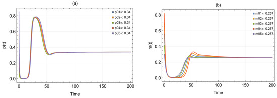
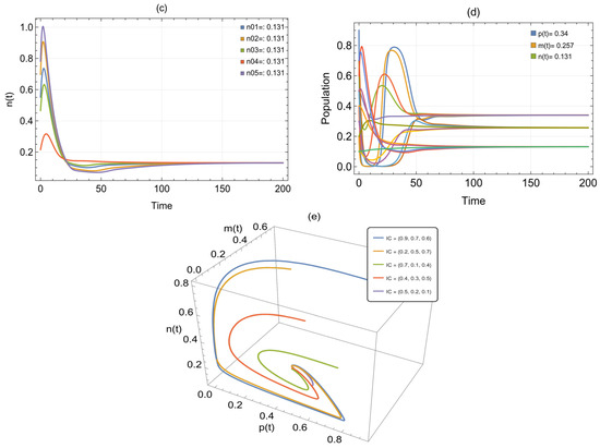
Figure 1. Trajectories of system (2) originating from different beginning positions and employing the parameters in Table 1. The trajectories illustrate the movements of the (a) prey, (b) infected prey, and (c) predator over time; (d) time series for ${\Phi }_4$; (e) 3D phase portrait of system (2).

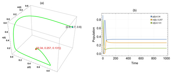
Figure 2. (a) Three-dimensional phase diagram of system (2). (b) The time series exhibits the trajectories of system (2) utilizing the parameters in Table 1 and showing convergence towards ${ \Phi }_4= (0.34, 0.257, 0.131)$.

We examined each variable and its impact on the system. Replacing the argument ${\tau }_1$, the system has three cases: the first one approaches a globally asymptotically stable positive point, ${ \Phi }_4 = \left(0.802, 0.073, 0.056\right)$, in the interval $\left(0.2, 1.28\right)$; the second one approaches ${ \Phi }_1 =\left(1,0,0\right)$ in the interval $\left(0,0.2\right]$; and the last one approaches ${ \Phi }_{2 } =\left(0.11, 0.378, 0\right)$ in the interval [1.28,1.9) (Figure 3).

Figure 3. The trajectories of system (2) utilizing the parameters in Table 1 and different ${\tau }_1$ values. Three-dimensional phase portrait and time series for the trajectories at (a,b) ${\tau }_1=0.256$, (c,d) ${\tau }_1=0.144$, and (e,f) ${\tau }_1=1.352$.

By replacing ${\tau }_3$ in the system, we found two approaches to globally asymptotically stable points: ${ \Phi }_{4 }=\left(0.554, 0.174, 0.088\right)$ in the period $\left(0,0.5\right)$ and ${ \Phi }_{1 }=\left(\mathrm{1,0},0,0\right)$ in the interval $[0.5,1.9)$ (Figure 4).

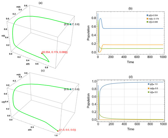
Figure 4. The trajectories of system (2) utilizing the parameters in Table 1 and different ${\tau }_3$ values. Three-dimensional phase portrait and time series for the trajectories at (a,b) ${\tau }_3=0.28$ and (c,d) ${\tau }_3=0.5$.

By substituting parameter ${\tau }_6$ into the system, we obtained two approaches to globally asymptotically stable points in the system: ${\Phi }_{4 }=\left(0.641, 0.141, 0.07\right)$ in the interval $\left(0,0.468\right)$ and ${\Phi }_{1 }= \left(1, 0, 0\right)$ in the interval $\left[0.468,1.9\right)$ (Figure 5).

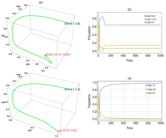
Figure 5. The trajectories of system (2) utilizing the parameters in Table 1 and different ${\tau }_6$ values. Three-dimensional phase portrait and time series for the trajectories at (a,b) ${\tau }_6=0.284$ and (c,d) ${\tau }_6=0.481$.

Figure 6 shows three approaches to globally asymptotically stable points when ${\tau }_7$ was changed in the system: ${ \Phi }_{4 }= \left(0.346, 0.238, 0.144\right)$ in the period $\left(0.001,0.214\right)$, ${ \Phi }_{3 }= \left(0.084, 0, 0.467\right)$ in the interval (0.214,1.9), and ${ \Phi }_{2 }= \left(0.289, 0.444, 0\right)$ in the interval (0,0.001].

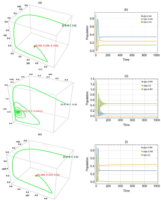
Figure 6. The trajectories of system (2) utilizing the parameters in Table 1 and different ${\tau }_7$ values. Three-dimensional phase portrait and time series for the trajectories at (a,b) $s_7=0.119$, (c,d) ${\tau }_7=0.986$, and (e,f). ${\tau }_7=0.001$.

By substituting parameter ${\tau }_8$ into the system, we obtained two asymptotic approaches: ${ \Phi }_{4 }=\left(0.406, 0.061, 0.26\right)$ in the period (1.66, 0.773) and ${ \Phi }_{2 }=\left(0.289, 0.444, 0\right)$ in the interval ($\mathrm{0,1.66}]$ (Figure 7).

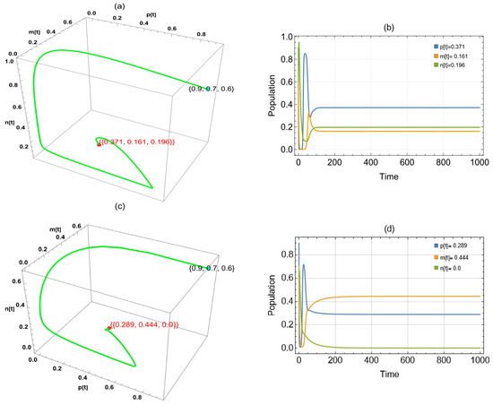
Figure 7. The trajectories of Equation (3) utilizing the parameters in Table 1 and different ${\tau }_8$ values. Three-dimensional phase portrait and time series for the trajectories at (a,b) ${\tau }_8=0.335$ and (c,d) ${\tau }_8=0.141$.

By substituting $s_9$ into the system, we obtained two approaches to globally asymptotically stable points: ${\Phi }_{4 }=\left(0.354, 0.213, 0.161\right)$ in the period $\left(0.057,0.142\right)$, ${ \Phi }_{3 }= \left(0.153, 0, 0.434\right)$ in the interval (0, 0.057], and ${\Phi }_{2 }=\left(0.289, 0.444, 0\right)$ in the interval [0.142, 1) (Figure 8).

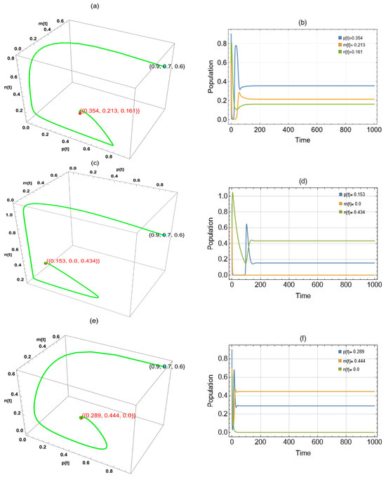
Figure 8. The trajectories of system (2) utilizing the parameters in Table 1 and different ${\tau }_9$ values. Three-dimensional phase portrait and time series for the trajectories at (a,b) ${\tau }_9=0.102$, (c,d) ${\tau }_9=0.022,$ and (e,f) ${\tau }_9=0.287$.

7. Discussion

We developed a mathematical model to investigate the disease dynamics in a system consisting of susceptible prey, infected prey, and a predator. The model includes key ecological and epidemiological dynamics, such as interspecies competition and cooperation among predators of different species. Fear was only represented as a reduction in the intrinsic growth rate of susceptible prey. This captures an important ecological process, but it simplifies a larger suite of behavioral effects of fear. In natural systems, fear could also lower the mock-up (rate of direct contact) and consequently lower disease transmission rate, or affect spatial movement and vigilant behaviors, and thus, affect predation pressure. Both potential outcomes will be moderated by stress effects on the disease susceptibility of the host. Fully accounting for and describing the effects of fear would require expanding the model to capture these routes; however, this adds considerable complexity to the model and will have to be addressed in future work. Disease transmission among prey occurs through direct interactions (contact), and the system boundedness was set to guarantee biologically realistic solutions. The theoretical results were validated by numerical simulations. The time series and phase portraits supported the theoretical predictions and provide insights into the mechanisms of disease spread, competition, and predation in the ecosystem. The results reveal how the interactions of ecology and epidemiology can change the stability of a population, leading to potentially complex dynamical behaviors.

The stability and bifurcation analyses show that fear is a significant ecological regulator: it decreases prey reproduction and infection opportunities and indirectly suppress predator persistence by limiting the available prey biomass. Thus, moderate fear can reduce the prevalence of disease without pushing predators to extinction, and excessive fear can destabilize the community by driving predators to extinction and allowing infection to dominate. These results have implications because they show that fear is both a shielding mechanism as well as a potential destabilizer, illustrating the need to include behavioral responses into ecological modeling to meaningfully understand ecosystems. Through numerical analysis, the presence of multiple equilibrium points was verified along with the conditions under which the system converges to a globally asymptotically stable state. This study highlights the importance of numerical simulation methods to gain a better understanding of system behaviors in contrast to purely analytical methods. Analyzing the effect of fear is an essential step in understanding how more complex models that include nonlinear effects and more complex interactions between different types evolve, as was shown in our study. The model assumes that fear slows the growth of susceptible prey, so fewer susceptible prey are available to be infected. This, in turn, lessens the transmission pressure and reduces the length of outbreaks. When fear is sufficiently strong, the disease cannot become established, leaving the system in a disease-free state. In cooperative hunting, an increased per capita success and energy gain allows the predators to survive even if prey are relatively scarce, increasing the rate of removal of infected prey, which bolsters the predator population further and expands the range of parameters for predator persistence. We also observed that cooperative hunting also influenced the prey. However, including fear in the system can lead to fundamental changes in the stability and behavior of the system.

Unlike past studies that addressed some combination of disease dynamics, fear effects, and/or cooperative hunting, our model incorporates all three mechanisms into a single eco-epidemiological model. By studying these different mechanisms together, we uncovered some new ecological implications (e.g., fear reduces prey growth but when prey die due to cooperative hunting, predation co-varyingly reduces disease persistence while the cooperative hunting enhances predator survival). These findings build on earlier models by incorporating a broader and more equivocal view of the process, capturing the complex interactions that can occur through behavioral, epidemiological, and ecological processes that affect final and future populations.

In ecological and epidemiological terms, and generally speaking, our results show that fear suppresses growth in prey, which leads to indirect suppression of disease transmission, and that cooperative hunting enhances predator survival and leads to quicker removal of diseased prey. Together, they promote stability, allowing all populations to coexist when the conditions are right. Overall, our model illustrates how behavioral responses and epidemiological processes together drive community dynamics and expands the boundaries of traditional predator–prey–disease models.

The system is deterministic and does not account for stochastic environmental fluctuations or random demographic events. Future work could incorporate stochastic perturbations, where methods such as stochastic Lyapunov functions are used to estimate extinction probabilities and compare deterministic versus stochastic thresholds. Because fear-induced behavioral changes may profoundly impact prey development and disease transmission, subsequent developments can incorporate fear-mediated functional responses to enhance realism.

All simulations or numerical studies were carried out in Mathematica, an excellent and powerful platform for our work, which was used to solve the system equations and obtain the graphical solutions.

References

- Kapur, J.N. Mathematical Modelling; John Wiley & Sons: New York, NY, USA, 1988. [Google Scholar]
- Farkas, M. Dynamical Models in Biology; Academic Press: Cambridge, MA, USA, 2001. [Google Scholar] [CrossRef]
- Haefner, J.W. Modeling Biological Systems: Principles and Applications, 2nd ed.; Springer: Berlin/Heidelberg, Germany, 2005. [Google Scholar] [CrossRef]
- Teschl, G. Ordinary Differential Equations and Dynamical Systems; American Mathematical Society: Providence, RI, USA, 2012; p. 140. [Google Scholar] [CrossRef]
- Fishwick, P.A. Handbook of Dynamic System Modeling; Chapman and Hall/CRC: Boca Raton, FL, USA, 2007. [Google Scholar] [CrossRef]
- Gershenfeld, N. The Nature of Mathematical Modeling; Cambridge University Press: Cambridge, UK, 1999. [Google Scholar]
- Zhang, H.; Yuan, X.; Zou, H.; Zhao, L.; Wang, Z.; Guo, F.; Liu, Z. The Spatiotemporal Dynamics of Insect Predator–Prey System Incorporating Refuge Effect. Entropy 2024, 26, 196. [Google Scholar] [CrossRef] [PubMed]
- Choh, Y.; Sabelis, M.W.; Janssen, A. Predatory interactions between prey affect patch selection by predators. Behav. Ecol. Sociobiol. 2017, 71, 66. [Google Scholar] [CrossRef] [PubMed]
- Ibrahim, L.R.; Bahlool, D.K. Modeling and analysis of a prey–predator–scavenger system encompassing fear, hunting cooperation, and harvesting. Iraqi J. Sci. 2025, 66, 2014–2037. [Google Scholar] [CrossRef]
- Abdullah, H.S.; Bahlool, D.K. The influence of fear and predator-dependent refuge on the dynamics of a harvested prey–predator model with disease in predator. Iraqi J. Sci. 2025, 66, 2455–2476. [Google Scholar] [CrossRef]
- Yaseen, R.M.; Mohsen, A.A.; Al-Husseiny, H.F. Improving the hepatitis viral transmission model’s dynamics by vaccination and contrasting it with the fractional-order model. Partial Differ. Equ. Appl. Math. 2024, 10, 100705. [Google Scholar] [CrossRef]
- Peacor, S.D.; Werner, E.E. The contribution of trait-mediated indirect effects to the net effects of a predator. Proc. Natl. Acad. Sci. USA 2001, 98, 3904–3908. [Google Scholar] [CrossRef]
- Agarwal, M.; Pathak, R. Influence of prey reserve in two preys and one predator system. Int. J. Eng. Sci. Technol. 2014, 6, 1–19. [Google Scholar] [CrossRef]
- Anitha, K.; Srinivas, M.N.; Madhusudanan, V. Stochastic and delay analysis of two preys and one predator ecological system with competition among preys and self interaction. Dyn. Syst. Applions. 2018, 2, 201–224. Available online: https://acadsol.eu/dsa/articles/27/2/1-1.pdf (accessed on 4 September 2025). [CrossRef]
- Haque, M.; Chattopadhyay, J. Role of transmissible disease in an infected prey-dependent predator–prey system. Math. Comput. Model. Dyn. Syst. 2007, 13, 163–178. [Google Scholar] [CrossRef]
- Venturino, E. Disease Spread among Hunted and Retaliating Herding Prey. Mathematics 2022, 10, 4397. [Google Scholar] [CrossRef]
- Al-Husseiny, H.F.; Ali, N.F.; Mohsen, A.A. The effect of epidemic disease outbreaks on the dynamic behavior of a prey–predator model with Holling type II functional response. Commun. Math. Biol. Neurosci. 2021, 2021, 72. [Google Scholar] [CrossRef]
- Banerjee, R.; Das, P.; Mukherjee, D. Global dynamics of a Holling type-III two-prey–one-predator discrete model with optimal harvest strategy. Nonlinear Dyn. 2020, 99, 3285–3300. [Google Scholar] [CrossRef]
- Kar, T.K.; Misra, S. Influence of prey reserve in a prey–predator fishery. Nonlinear Anal. Theory Methods Appl. 2006, 65, 1725–1735. [Google Scholar] [CrossRef]
- Pratama, R.A.; Ruslau, M.F.V.; Suryani, D.R.; Loupatty, M. Dynamics twin cannibalism of two predator and two prey system with prey defense. MATEC Web Conf. 2022, 372, 02008. [Google Scholar] [CrossRef]
- Liu, J.; Hu, J.; Yuen, P.; Li, F. A Seasonally Competitive M-Prey and N-Predator Impulsive System Modeled by General Functional Response for Integrated Pest Management. Mathematics 2022, 10, 2687. [Google Scholar] [CrossRef]
- Peng, C.; Jiang, J. Dynamical Regimes in a Delayed Predator–Prey Model with Predator Hunting Cooperation: Bifurcations, Stability, and Complex Dynamics. Modelling 2025, 6, 84. [Google Scholar] [CrossRef]
- Berardo, C.; Bulai, I.M.; Venturino, E. Interactions Obtained from Basic Mechanistic Principles: Prey Herds and Predators. Mathematics 2021, 9, 2555. [Google Scholar] [CrossRef]
- Belvisi, S.; Venturino, E. An ecoepidemic model with diseased predators and prey group defense. Math. Biosci. Eng. 2013, 34, 144–155. [Google Scholar] [CrossRef]
- Kar, T.K.; Batabyal, A. Stability and bifurcation of a prey-predator model with time delay. C. R. Biol. 2009, 332, 642–651. [Google Scholar] [CrossRef]
- Lan, L.H. Predator–prey system with the effect of environmental fluctuation. VNU J. Sci. Math. Phys. 2014, 30, 1–14. Available online: https://js.vnu.edu.vn/MaP/article/view/751 (accessed on 4 September 2025).
- Alebraheem, J. Dynamics of a Predator–Prey Model with the Effect of Oscillation of Immigration of the Prey. Diversity 2021, 13, 23. [Google Scholar] [CrossRef]
- O’Connor, N.E.; Emmerson, M.C.; Crowe, T.P.; Donohue, I. Distinguishing between direct and indirect effects of predators in complex ecosystems. J. Anim. Ecol. 2013, 82, 438–448. [Google Scholar] [CrossRef] [PubMed]
- Meng, X.-Y.; Xiao, L. Hopf bifurcation and Turing instability of a delayed diffusive Zooplankton–Phytoplankton model with hunting cooperation. Int. J. Bifurc. Chaos 2024, 34, 2450090. [Google Scholar] [CrossRef]
- Li, Y.; Ding, M. Impact of hunting cooperation in predator and anti-predator behaviors in prey in a predator–prey model. Math. Methods Appl. Sci. 2024, 48, 237–252. [Google Scholar] [CrossRef]
- Tao, W.; Wang, Z.-A. Global well-posedness and Turing–Hopf bifurcation of prey-taxis systems with hunting cooperation. Eur. J. Appl. Math. 2025, 36, 1121–1147. [Google Scholar] [CrossRef]
- Peng, M.; Lin, R.; Zhang, Z.; Huang, L. The dynamics of a delayed predator-prey model with square root functional response and stage structure. Electron. Res. Arch. 2024, 32, 3275–3298. [Google Scholar] [CrossRef]
- Naseer, A.H.; Bahlool, D.K. Dynamics of an Intraguild Predation Food Web Cooperation Model Under the Influence of Fear and Hunting. Computation 2025, 13, 128. [Google Scholar] [CrossRef]
- Waezizadeh, T.; Mehrpooya, A. A stochastic model for dynamics of two populations and its stability. In Proceedings of the 47th Annual Iranian Mathematics Conference (AIMC47), Karaj, Iran, 28–31 August 2016; Volume 10681071. [Google Scholar]
- Ferreira, J.D.; Molina, W.L.; Perez, J.J.; González, A.P. Stability and bifurcation analysis in predator–prey system involving Holling type-II functional response. Math. Biosci. Eng. 2025, 22, 2559–2594. [Google Scholar] [CrossRef]
- Diuk-Wasser, M.A.; VanAcker, M.C.; Fernandez, M.P. Impact of land use changes and habitat fragmentation on the eco-epidemiology of tick-borne diseases. J. Med. Entomol. 2020, 58, 1546–1564. [Google Scholar] [CrossRef]
Disclaimer/Publisher’s Note: The statements, opinions and data contained in all publications are solely those of the individual author(s) and contributor(s) and not of MDPI and/or the editor(s). MDPI and/or the editor(s) disclaim responsibility for any injury to people or property resulting from any ideas, methods, instructions or products referred to in the content. |
© 2025 by the authors. Licensee MDPI, Basel, Switzerland. This article is an open access article distributed under the terms and conditions of the Creative Commons Attribution (CC BY) license (https://creativecommons.org/licenses/by/4.0/).