Enhanced Drag Force Estimation in Automotive Design: A Surrogate Model Leveraging Limited Full-Order Model Drag Data and Comprehensive Physical Field Integration

Abstract

In this paper, a novel surrogate model for shape-parametrized vehicle drag force prediction is proposed. It is assumed that only a limited dataset of high-fidelity CFD results is available, typically less than ten high-fidelity CFD solutions for different shape samples. The idea is to take advantage not only of the drag coefficients but also physical fields such as velocity, pressure, and kinetic energy evaluated on a cutting plane in the wake of the vehicle and perpendicular to the road. This additional “augmented” information provides a more accurate and robust prediction of the drag force compared to a standard surface response methodology. As a first step, an original reparametrization of the shape based on combination coefficients of shape principal components is proposed, leading to a low-dimensional representation of the shape space. The second step consists in determining principal components of the x-direction momentum flux through a cutting plane behind the car. The final step is to find the mapping between the reduced shape description and the momentum flux formula to achieve an accurate drag estimation. The resulting surrogate model is a space-parameter separated representation with shape principal component coefficients and spatial modes dedicated to drag-force evaluation. The algorithm can deal with shapes of variable mesh by using an optimal transport procedure that interpolates the fields on a shared reference mesh. The Machine Learning algorithm is challenged on a car concept with a three-dimensional shape design space. With only two well-chosen samples, the numerical algorithm is able to return a drag surrogate model with reasonable uniform error over the validation dataset. An incremental learning approach involving additional high-fidelity computations is also proposed. The leading algorithm is shown to improve the model accuracy. The study also shows the sensitivity of the results with respect to the initial experimental design. As feedback, we discuss and suggest what appear to be the correct choices of experimental designs for the best results.

1. Introduction

In automotive engineering, drag reduction is a crucial step aimed at improving aerodynamics to increase vehicle range. As it has a major impact on the architecture and design of the product, aerodynamics is among the first performance to be studied and optimized. The design convergence is split between physical and numerical testing. While physical testing allows for faster iteration and more precise results, it is limited by the possibilities offered in a wind tunnel facility. It is often used in the final stages of development, with fine-tuning and approval in mind. On the contrary, numerical simulation is used very early in a project to initiate the design convergence, by eliminating non-compliant design and proposing solutions to improve the aerodynamic performance. However, each simulation is time-consuming and costly. A typical automotive simulation involves turbulence models and unsteady computation, leading to restitution delay in hours. Shape optimization is often used in this context to propose small alterations at various locations to improve the global performance. The design variables are mostly defined by the three-dimensional CAD shape parametrization. For standard vehicles, the admissible design domain can be rather big with numerous parameters. Among the reference computational approaches for shape optimization, one can distinguish two main families of methods: gradient-based methods and surrogate modeling techniques.

1.1. Gradient-Based Approaches

The first family considers gradient-based or descent-based optimization algorithms. These iterative methods require at least the evaluation of the gradient of the cost function (the drag coefficient in the context of this paper) with respect to the shape variables. For the evaluation of the gradient, adjoint-based methods have marked significant progress in optimization techniques. The calculation of the gradient using the adjoint method was introduced by Lions [1], then further developed, e.g., by Pironneau [2] and Jameson [3,4]. The key feature of the adjoint method is that the numerical complexity to evaluate the gradient does not depend on the number of variables, enabling its application for high-dimensional parametric problems. Although extensively utilized in the aeronautical field, this method is still relatively underused in automotive aerodynamics. The adjoint method requires the development of an additional code, the so-called adjoint code. The case of adjoint methods for unsteady computations is a harder task since the primal time-dependent solution has to be stored. In this context, we mention the work by Cheylan et al. [5], where an adjoint solver was derived from a Lattice Boltzmann Method code for the Navier–Stokes equations, including a large eddy simulation (LES) turbulence model. However, adjoint-based shape optimization is limited in practical applications due to the iterative and computationally expensive nature of CFD simulations. This makes it difficult to meet the demands of fast, interactive design optimization, where rapid feedback is essential. Moreover, in the automotive industry, design is often driven by aesthetic constraints, which are difficult to quantify mathematically. This makes it challenging to integrate them directly into an optimization process.

1.2. Surrogate Modeling

The second family of methods groups together all the surrogate modeling techniques. A surrogate model is based on approximation methods such as regression to build an easy-to-compute approximate cost function. For that, a design of computer experiment (DoCE) is used. The first step is to choose a sampling strategy of the admissible design space. Then, high-fidelity (HF) computations are run to evaluate the cost function at these sample points. The so-called Response Surface Methodology (RSM) is widely used in the Computer-Assisted Engineering community because of the simplicity in its design and setup. RSM can be built with various approximation methods such as Radial Basis Function [6,7], Gaussian Process [8], or AI tools such as regression-based Artificial Neural Networks [9].

However, for high-dimensional design problems, a significant number of HF computations is needed. The Latin Hypercube Sampling (LHS) strategy allows to sample a hypercube domain with a number of samples equal to the dimension d. However, it is known to be generally insufficient for obtaining an accurate response surface. An acknowledged empirical law is to consider a number of samples equal to d times a constant (between 3 and 5 for aerodynamic studies). In the automotive industry, this leads to an unrealistic budget of computations. This is why innovative methods that require fewer input samples, such as the approach proposed in this paper, are being explored. By approximating the results of expensive and time-consuming CFD simulations, surrogate models enable the creation of rapid, interactive design tools that significantly speed up the evaluation and optimization process.

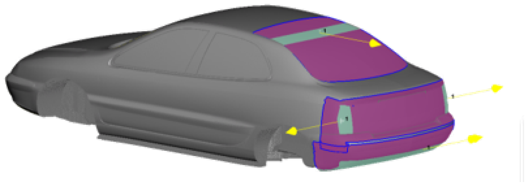
1.3. Shape Parametrization

Another important topic is the way to parametrize the car shapes. The performance of the optimization process can strongly depend on the shape parametrization. Some CAD parameter variations may have a very weak influence on the drag value. Of course, the “true” manifold of parameters of interest is not known a priori. Moreover, for technical and practical reasons, engineers may only consider and manipulate meshed geometries as “objects-of-study”. For different CAD samples, the mesh software may produce meshes with different mesh connectivity. Sometimes, the CAD parameters change during the study. If the surrogate model is built with those initial parameters, any changes would necessitate retraining the model. In that case, one has to imagine a reparametrization of the vehicle shapes from the available meshes. This will be discussed in this paper.

1.4. Adding Information from Available Volume Fields

As mentioned above, surface response methodologies can build regression functions of drag coefficients from various shape parameter sample HF computations. By solely retrieving aerodynamic coefficients from high-fidelity calculations, a significant part of the information contained in the results is lost. It appears advantageous to leverage ancillary information such as velocity fields, pressure distributions, or kinetic energy. As drag coefficients are correlated with these fields, one can expect more accurate drag force predictions providing correlated information. Volume fields defined on meshes are highly dimensional by nature. In order to obtain a low-dimensional representation of them, dimensionality reduction techniques such as principal component analysis (PCA [10]), proper orthogonal decomposition (POD [11]), locally linear embedding (LLE [12]), and multidimensional scaling or neural-based encoders [9] can be used. In the case of parametric problems, one can combine both dimensionality reduction with response surface methods to predict the reduced variables to obtain a parametric reduced-order model of the field.

As presented later on in Section 2 (methodology), the whole drag force is the integral of the normal stresses exerted onto the vehicle skin. Thus, the drag force is a function of the pressure field and the velocity gradient. A way to derive a more physical drag force is to achieve a low-order surrogate model of the skin normal stresses. Another way to evaluate the drag force is to adopt the so-called far-field approach, where the drag force can be well-approximated by the integral of a difference of momentum fluxes over an arbitrary cutting plane, preferably located in the wake of the vehicle (this will be detailed and explained in Section 2). In this case, the drag force depends on the pressure distribution, velocity, and kinetic energy fields. A key advantage of far-field formulas is that the cutting plane can be the same for all car shapes of interest, allowing for easier principal component analysis and dimensionality reduction.

1.5. Scope, Objectives, and Structure of the Paper

Classical RSM for drag prediction often require extensive input data, with hundreds to thousands of evaluations (simulations) needed to achieve acceptable accuracy. This evaluation-intensive requirement is not compatible with industrial processes where development times are short. Generating large datasets is not only time-consuming but also financially expensive. In the literature, there is a lack of surrogate models trained with a limited amount of input data, ideally of the order of the number of shape parameters. A big shortcoming of RSM is that it usually only makes use of quantities of interest (here, drag forces) that are often scalar, with all the physical fields being lost. Moreover, many current surrogate models are designed for predicting the drag of cars with significant geometric modifications or even different vehicle models. These models are useful in the early stages of development to assess the bulk geometry. However, during the fine styling phase where modifications are minimal (often just a few centimeters), these models become less effective. There is a clear gap in the literature regarding models that can accurately predict drag for such small geometric changes and with only limited input data. To overcome this scientific challenge, we have to parameterize the car shape in such a way that drag force responses are strongly correlated to the shape parameters. There is also the constraint of low-dimensional representation since the dataset is made of few evaluations and one can only consider few degrees of freedom for the identification of the operator that maps shape into drag force.

These constraints lead us to consider an enhanced surrogate model with the following features:

• Low-dimensional reparametrization of the vehicle geometry.
• Incorporation of physical fields to enrich the data and raise the information content without additional CFD computations; this represents the biggest difference from traditional methods.
• Reliance on physical formulas for calculating drag forces.
• Ability to compute sensitivities, i.e., accuracy for small geometry variations.

Let us also emphasize that the “limited evaluations” constraint sets the work apart from methods relying on extensive datasets (like deep neural networks and related data-intensive ML approaches). In addition, the use of artificial data generative AI systems cannot meet the requirement of accuracy for slight geometric changes (final fine styling phase).

The paper is organized as follows. Section 2 is dedicated to the methodology of the method. It includes integral formulas of drag force (Section 2.1), the shape encoding and reparametrization (Section 2.2), the low-order representation of the momentum formula in the wake cutting plane (Section 2.3), the definition of the drag surrogate model (Section 2.4), and its use for a new “query” shape (Section 2.6). Section 3 gathers all the numerical experiments and validations conducted. The paper ends with concluding remarks and perspectives in Section 4.

1.6. Related Works

This section is intended to provide an overview of the recent literature and related works in the context of surrogate modeling and machine learning methods for automotive drag force prediction. In aerodynamic studies, the performance of a design is often evaluated based on the drag coefficient. Some models only predict this scalar coefficient, while others predict the entire flow field, from which the drag is computed. Both approaches require extensive input data to achieve high prediction accuracy. Two main categories of models emerge in the literature: those used in early-phase project development with a broad range of shape variations and those designed for more specific geometry variations. The ShapeNet dataset https://shapenet.org/ (accessed on 1 June 2023) is commonly employed for training models that need to handle diverse car shapes. For instance, ref. [13] proposed a method using the Gaussian Process with optimized weights to predict the drag coefficient along with pressure and velocity field surrounding simplified 3D cars (without spoilers, tires, and side mirrors) of this dataset. Car shapes are parameterized using a Polycube map, which allows for a fixed-length representation of all shapes. The positions of PolyCube mesh surface points are used for the GP model. Trained with 889 shapes, the model’s prediction accuracy improves as the training set size increases, with the error decreasing from 5.4% for 100 samples to 3.4% for 889 samples. Additionally, the model achieves an average Mean Squared Error of 0.48 on velocity and 8.1 on pressure when trained with the full dataset. A manifold-based approach was presented in [14], where authors use Locally Linear Embedding to predict the drag of 3D car shapes. The method assumes that the drag coefficient of a car can be obtained through the linear combination of five neighboring cars in the manifold of car shapes. To build the manifold, the signed distance function of 60 car shapes from the ShapeNet dataset was used. An overall average relative percent error of 11.5% was achieved with this approach. In [15], the authors applied a similar method to estimate the airflow around the vehicle using a reduced input dataset. The model was constructed using the signed distance function of 70 car shapes, including various types like sedans and sports cars. The model achieved an $L^2$ error on the velocity field ranging from 0.56% to 1%, depending on the car type. Neural Networks (NN), especially Convolutional Neural Networks (CNN), have been widely adopted due to their efficacy in extracting spatial features. For instance, ref. [16] proposed an improved ResNeXt model [17] that uses 2D depth and normal renderings to represent 3D car geometries. By training on 9070 shapes from ShapeNet, their model achieved an overall average drag prediction error of 2.4%. The Shapenet dataset was also used by [18] to train a coordinate-based multilayer perceptron to predict the flow field around a 2D car profile. Trained on 1812 profiles, derived from the central vertical cross-section of 3D shapes of the ShapeNet dataset, the model achieved an average MSE of 7.15% for drag prediction. Similarly, [19] used Convolutional Neural Networks on arbitrary 2D primitives to predict airflow around 2D car silhouettes. This model returned a prediction error of 15.34%. In [20], a U-Net [21] architecture was employed to predict the drag coefficients and flow field of car shapes from the geometry [22]. This model uses a signed distance function for 3D geometry representation and is trained on up to 10,080 samples, achieving a maximum absolute error of approximately 2.5% in drag prediction and 2.8% on the $L^2$ error of field prediction. Alternatively, a Geodesic Convolutional Neural Network [23] was used in [24] to predict pressure and velocity distribution on the surface of a 3D car. As in [13], the car geometries were remeshed using a Polycube map for consistent representation. The model trained on approximately 2000 randomly generated car shapes reported an accuracy of 51% for new prediction. The accuracy of the model can reach up to 70% when the model training dataset is augmented with 54 real car shapes. This Geodesic Convolutional Neural Network was used in [25] for drag optimization. The GCNN-based approach outperforms traditional methods like Kriging in creating a surface response for optimal drag coefficient prediction. However, no details on the error or accuracy of the surface response were provided by authors. An optimization study was also presented in [26], where the authors introduced MeshSDF, a model designed for the generation and optimization of 3D geometries. The model learns from point cloud representations of the 3D geometry and uses a CNN to predict the pressure field over the shape. Trained on 1400 car shapes from the ShapeNet dataset, the model was employed to generate optimized shapes that minimize pressure drag from an initial configuration. However, the authors provided no details on the accuracy of their pressure field predictions or the resulting drag estimations.

Another category of models focuses on studying specific geometric variations for fine styling adjustments. These models aim to predict drag or flow fields when a defined car geometry undergoes specific modifications. This is the focus of our paper, as such models are important for optimizing aerodynamic performance. Despite their importance, there is limited research on applying these types of models within the automotive industry. In [27], a mathematical model was built to generate new silhouettes of a sedan parameterized with 21 design parameters and then estimate their drag coefficient. The mathematical model was constructed using a two-step procedure to predict the drag coefficient from the coordinates of 52 control points. First, Principal Component Analysis (PCA) was applied to reduce the number of variables used for the geometry representation. These principal components were then used in a linear regression model to predict the drag coefficient. The performance of the regression model for drag prediction was evaluated for different training sample sizes ranging from 100 to 1000. As the input sample size increased, the mean absolute percentage error decreased from 13.86% to 9.49%. For the largest sample size, 70% of the predictions had an error below 10%. However, the error can still reach up to 65% for certain silhouette types. Scaling up to 3D geometries, a Radial Basis Function was used in [28] to map design shape parameters to the drag coefficient of a 3D car with 12 shape parameters. Initially, with 164 high-fidelity evaluations from Latin hypercube sampling, the model achieved a 3.7% prediction error for the optimal shape. By using an Adaptive Multi-Scale RSM methodology, which refines the response surface iteratively, the error was reduced to less than 1% with increased sample sizes (280 to 480). This approach also makes the model less sensitive to the number and distribution of input samples compared to traditional RSM methodologies. Closest to our work, ref. [29] proposes a model that combines Proper Orthogonal Decomposition (POD) reduction with kriging interpolation to evaluate pressure and velocity fields on the surface of a car. In their approach, POD was applied to the snapshot matrix of results from a Detached Eddy Simulation (DES) for a car shape with three parameters. A kriging model was then used to interpolate the POD basis coefficients based on shape modifications. The model was trained using multiple datasets with varying distributions and input sample sizes ranging from 8 to 38. As the number of input samples increased, the relative error decreased from 2.3% to 1.1% for pressure prediction and from 2.9% to 1.7% for viscosity prediction. With a Latin hypercube dataset of 20 samples, the mean error in drag prediction using the estimated fields is 0.3%. Additionally, a variable fidelity approach was explored to enhance the high-fidelity DES snapshots with lower fidelity Reynolds-Averaged Navier–Stokes (RANS) snapshots. However, this approach did not yield better prediction results for the test case considered.

The reviewed approaches highlight the use of extensive input data for developing effective models in automotive drag force prediction. They also reveal a notable gap in research concerning fine-tuning models for specific geometric variations.

2. Methodology

2.1. Drag Force Evaluation Methods

Aerodynamic simulations of automotive vehicles are conducted at very high Reynolds numbers, typically of the order ${10}^7$, involving thin boundary layers and developed turbulence. To address these high-Reynolds-number flows, the solver relies on the Large Eddy Simulation (LES) method. LES is a numerical modeling approach aimed at directly capturing the large unsteady turbulent structures. Furthermore, it is combined with a Smagorinsky subgrid scale (SGS) model as the closure model. This combination enables the representation of turbulent features at a smaller scale than the primary grid resolution, thereby enhancing the precision of the models. These two concurrent approaches empower the solver to faithfully represent turbulent flows across various scales.

The evaluation of the drag force $f_x$ can then be carried out through the following equations [30,31]:

$$\mathit{f}={\int \int }_{S_v}\left((p-p_0)\mathit{n}-\tau ·\mathit{t}\right)d\sigma ,f_x=\mathit{f}·\widehat{\mathit{x}}$$

(1)

where p represents the static pressure, $p_0$ denotes the infinite unperturbed pressure, $\widehat{\mathit{x}}$ is the unit vector in the x direction, $\tau$ represents the viscous stress tensor, n stands for the unitary normal vector on the vehicle’s surface $S_v$, and $\mathit{t}$ is the tangential unit vector. The viscous stress tensor is calculated as $\tau =\nu (\nabla \mathit{u}+\nabla {\mathit{u}}^T)$, with $\nu$ representing the kinematic viscosity and $\nabla \mathit{u}$ denoting the velocity gradient tensor.

Rather than determining aerodynamic forces through the integration of stresses on the vehicle surface, the drag force can also be evaluated on another “virtual” surface into the fluid domain. Assuming a bounding domain that is far enough from the vehicle, the drag force can be estimated on a fixed rear cutting plane $S_{cp}$, which is orthogonal to $\widehat{\mathit{x}}$, located in the wake of the vehicle according to the so-called far-field formula, also known as the Onorato formula [32]:

$$f_x={\int \int }_{S_{cp}}\left(p_0-p+\rho [u_0{u}_x-{\left(u_x\right)}^2]\right)dS.$$

(2)

Here, $\rho$ represents the fluid density, $u_0$ is the freestream velocity, and $u_x$ is the velocity component in the direction of interest x. This will allow us to obtain snapshot fields that are defined on the grid $S_{cp}$ that do not depend on the vehicle shapes. The surface drag coefficient is computed from the aerodynamic force $f_x$ using formula [31]: $C_{d}A=f_x/\left({\displaystyle \frac{1}{2}}{\rho }_0{u}_0^2\right)$.

Because of the use of an LES turbulence model (see [33]), the Navier–Stokes solver returns unsteady solutions. However, when evaluating vehicle performance, metrics such as drag coefficient $C_{d}A$ are usually searched as constant values. The LES-based Navier–Stokes solutions are expected to reach a stationary flow after a transient phase, in the sense of a stationary stochastic process (stationary flow being averaged over a suitable time window). Thus, the drag coefficient $C_{d}A$ is typically computed from time-averaged quantities to return an expectation value. When computing mean far-field drag, careful attention must be paid to evaluate mean values of nonlinear terms like ${\left(u_x\right)}^2$.

The shape-parametrized reduced-order surrogate model proposed in this paper is composed of three stages: (i) shape encoding; (ii) extraction of proper orthogonal modes on the cutting plane; (iii) surrogate model of force density and drag force. In what follows, we present details of the three stages.

2.2. Shape Encoding

In the context of shape design optimization in automotive engineering, the assessment of performance often requires the evaluation of numerous geometrical variations of the vehicle through the numerical design of the experiment. To generate deformed geometries from a reference one, a direct morphing approach can be used. Local regions of reference geometry are transformed by defining a control area, where specific displacements are imposed; a free area, which is free to move; and a fixed area, which remains stationary during the morphing process (Figure 1). Assume that the shape of the vehicle depends on p CAD parameters ${\left({\mu }_k\right)}_{k=1,\dots ,p}$ that are gathered into a vector $\mathit{\mu }$. The domain of admissible shape parameters $\mathit{\mu }$ is denoted by $\mathcal{M}\subset {\mathbb{R}}^p$. In the sequel, the car shape for parameter $\mathit{\mu }$ will be denoted by $\underline{S}(.,\mathit{\mu })$. It will be assumed that each shape $\underline{S}(.,\mathit{\mu })$ is a slight variation of a reference shape denoted by ${\underline{S}}^{ref}(.)=\underline{S}(.,{\mathit{\mu }}^{ref})$.

Figure 1. Morphing regions on the well-known Ahmed body with one CAD parameter acting on the global height. Control areas are colored in green, free area in purple, and the boundary areas in blue.

To capture as much information as possible from the entire 3D shape and to be able to discriminate different admissible shapes, it is important to have a more informative and discriminating descriptor, able to characterize the principal components of geometrical variation. For efficiency purposes, such a shape encoding also has to be set up in a rather low-dimensional space.

The procedure used in the present work is explained in the sequel. It is assumed that the morphed geometry $\underline{S}(.,\mathit{\mu })$ is a slight variation from the reference surface ${\underline{S}}^{ref}(.)$. It can be characterized by a shape displacement vector field $\underline{\delta }(·,\mathit{\mu })\in {\left[L^2\left({\underline{S}}^{ref}\right)\right]}^3$ evaluated on the reference shape:

$$\underline{S}(·,\mathit{\mu })={\underline{S}}^{ref}(·)+\underline{\delta }(·,\mathit{\mu }).$$

(3)

The idea is to approximate all the admissible displacements in a rather low-dimensional vector space defined by a suitable orthogonal reduced basis. This can be performed, for example, from a method of snapshots of shapes.

Let ${\left\{\underline{S}(.,{\mathit{\mu }}^k)\right\}}_{k=1,\dots ,N_s}$ be a set of $N_s$ precomputed deformed shapes from a suitable CAD parameter sampling $\{{\mathit{\mu }}^1,\dots ,{\mathit{\mu }}^{N_s}\}$. From these shape snapshots, it is easy to find an orthogonal basis ${\underline{q}}_{\ell }(.)\in {\left[L^2\left({\underline{S}}^{ref}\right)\right]}^3$, $\ell =1,\dots ,K$, $K\le N_s$, either by means of a principal component analysis (PCA) or more simply by means of a Gram–Schmidt (GS) orthogonalization procedure. If $N_s$ is big enough, it is preferable to apply a PCA to find the K principal components, expecting that $K<N_s$. In the case of limited data with $N_s$ being small, one can consider $K=N_s$ and simply use the GS algorithm (i.e., QR factorization in the discretized context). Thus, for a query parameter vector $\mathit{\mu }\in \mathcal{M}$,

$$\underline{S}(·,\mathit{\mu })\approx {\underline{S}}^{ref}(.)+\sum _{\ell =1}^K{\nu }_{\ell }\left(\mathit{\mu }\right){\underline{q}}_{\ell }(·).$$

(4)

The linear combination coefficients ${\left({\nu }_{\ell }\left(\mathit{\mu }\right)\right)}_{\ell =1,\dots ,K}$ provide a set of descriptors of the shape $\underline{S}(.,\mathit{\mu })$. They are computed from the orthogonal projection of $\underline{\delta }(.,\mathit{\mu })$ onto the vector space spanned by the basis functions ${\mathit{q}}_{\ell }(·)$:

$${\nu }_{\ell }\left(\mathit{\mu }\right)={\left(\underline{\delta }(·,\mathit{\mu }),{\underline{q}}_{\ell }\right)}_{{\left[L^2\left(S^{ref}\right)\right]}^3}.$$

(5)

The feature vector $\mathit{\nu }\left(\mathit{\mu }\right)$ then serves as the new global shape descriptor to encode the geometry $\underline{S}(.,\mathit{\mu })$. This approach enables the creation of new shape descriptors that offer more descriptive information than the CAD parameters. By leveraging the detailed information captured at the local level from local features, this method provides a comprehensive representation of the overall shape, resulting in a more informative and nuanced global shape descriptor set.

Discretized Formalism

For computational purposes, any car shape is discretized thanks to a Finite Element (FE) triangular mesh as triangular elements are better suited for meshing complex geometries, such as detailed 3D car models. Let us assume a shape triangulation made of $N_v$ vertices, $N_v>>1$. The FE displacement fields $\underline{\delta }(.,\mathit{\mu })$ as well as the orthogonal fields ${\underline{q}}_{\ell }(.)$ are stored as large vectors ${\mathit{\delta }}_{\mu }$ and ${\mathit{q}}_{\ell }$, respectively. The shape encoding algorithm is the following:

• Offline stage: assume that a snapshot database of shape displacements

  $$D=\left[{\mathit{\delta }}_{{\mu }^1},{\mathit{\delta }}_{{\mu }^2},\dots ,{\mathit{\delta }}_{{\mu }^{N_s}}\right]\in {\mathbb{R}}^{3N_v\times N_s}$$

  is available. From an SVD analysis or a QR factorization of D, compute an orthogonal reduced basis ${\mathit{q}}_1,\dots ,{\mathit{q}}_K\in {\mathbb{R}}^{3N_v}$. Define the matrix,

  $$Q=\left[{\mathit{q}}_1,\dots ,{\mathit{q}}_K\right]\in {\mathbb{R}}^{3N_v\times K};$$
• Online stage: for a query CAD parameter $\mathit{\mu }$, compute a mesh of the shape $\underline{S}(;,\mathit{\mu })$. Then, compute the discrete displacement field ${\mathit{\delta }}_{\mu }$ and the POD coefficients vector,

  $$\begin{array}{c}\hfill \mathit{\nu }\left(\mathit{\mu }\right)=Q^T{\mathit{\delta }}_{\mu }\in {\mathbb{R}}^K.\end{array}$$

  (6)

Remark that if $N_s$ is small and the QR factorization $D=QR$ is used (in this case $K=N_s$), then

$$R=Q^{T}D\in {\mathbb{R}}^{K\times K}$$

is the matrix of the POD coefficients vector of each displacement vector ${\mathit{\delta }}_{{\mu }^1},{\mathit{\delta }}_{{\mu }^2},\dots ,{\mathit{\delta }}_{{\mu }^{N_s}}$ of D.

2.3. Knowledge Extraction and Reduced-Order Representation in the Cutting Plane

As already seen in the previous section, for a deformed shape $\underline{S}(.,\mathit{\mu })$, the aerodynamic drag can be estimated by integrating the physical scalar field

$$\kappa (.,\mathit{\mu })\stackrel{\mathrm{def}}{=}{p}_0-p(.,\mathit{\mu })+\rho [u_0{u}_x(.,\mathit{\mu })-u_x^2(.,\mathit{\mu })]$$

over a cutting plane $S_{cp}$ using the far-field formula:

$$C_{d}A\left(\mathit{\mu }\right)={\displaystyle \frac{1}{\frac{1}{2}{\rho }_0{u}_0^2}}{\int \int }_{S_{cp}}\kappa (.,\mathit{\mu })d{S}_y.$$

(7)

The quantity $\kappa (.,\mathit{\mu })\in L^2\left(S_{cp}\right)$ can be seen as the drag force density per unit surface over the cutting plane $S_{cp}$. As each new shape is a slight deformation of the reference shape, the resulting flow field is also a variation of that of the reference configuration. Then, the field force density $\kappa (·,\mathit{\mu })$ can be computed as the reference one plus a deviation $\Delta \kappa (·,\mathit{\mu })$:

$$\kappa (.,\mathit{\mu })={\kappa }^{ref}(.)+\Delta \kappa (.,\mathit{\mu }).$$

(8)

Once again, from the different snapshot solutions ${\left\{\kappa (.,{\mathit{\mu }}^k)\right\}}_{k=1,\dots ,N_s}$ previously computed with a high-fidelity CFD solver, one can extract an orthogonal reduced basis ${\psi }_{\ell }(.)\in L^2\left(S_{cp}\right)$, $\ell =1,\dots ,K$. This allows us to approximate the variation $\Delta \kappa (.,\mathit{\mu })$ in a low-dimensional vector space spanned by the orthogonal modes ${\psi }_{\ell }$, i.e.,

$$\Delta \kappa (.,\mathit{\mu })\approx \sum _{\ell =1}^K{b}_{\ell }\left(\mathit{\mu }\right){\psi }_{\ell }(.).$$

(9)

For the numerical implementation, the cutting plane is discretized using a Cartesian mesh or a Finite Element mesh composed of $N_{cp}$ nodes. The FE discrete fields $\kappa (.,\mathit{\mu })$ as well as the orthogonal basis ${\left({\psi }_{\ell }(.)\right)}_{\ell }$ are stored as large vectors ${\mathit{\kappa }}_{\mu }$ and ${\mathit{\psi }}_{\ell }$, respectively. The variation fields $\Delta \kappa (.,\mathit{\mu })$ are also stored as vectors $\Delta {\mathit{\kappa }}_{\mu }={\mathit{\kappa }}_{\mu }-{\mathit{\kappa }}^{ref}$. Then, the algorithm is as follows:

• Compute the snapshot matrix $U\in {\mathbb{R}}^{N_{cp}\times N_s}$ of field forces by collecting results of the high-fidelity CFD solver for the $N_s$ training shapes:

  $$U=\left[\begin{array}{ccc}\Delta {\mathit{\kappa }}_{{\mu }^1},& \cdots ,& \Delta {\mathit{\kappa }}_{{\mu }^{N_s}}\end{array}\right].$$

  (10)
• Extract the modes ${\mathit{\psi }}_{\ell }\in {\mathbb{R}}^{N_{cp}}$, $\ell =1,\dots ,K$ by performing either principal component analysis or QR factorization of matrix U, depending on the number of snapshots. Then, define the matrix,

  $$P=[{\mathit{\psi }}_1,...{\mathit{\psi }}_K]\in {\mathbb{R}}^{N_{cp}\times K}.$$
  For very limited snapshot data, it is preferable to use a QR factorization. In this case, we have $K=N_s$ and $U=PT$ with $T\in {\mathbb{R}}^{K\times K}$, an upper triangular matrix. Since the matrix P is semi-orthogonal, we have $T=P^{T}U$.

2.4. Parametric Surrogate Model

Equations (8) and (9) invite us to search $\kappa (.,\mathit{\mu })$ in the form

$$\kappa (.,\mathit{\mu })={\kappa }^{ref}(.)+\sum _{\ell =1}^K{b}_{\ell }\left(\mathit{\mu }\right){\psi }_{\ell }(.)$$

for a new query vector $\mathit{\mu }$, with corresponding shape $S(.,\mathit{\mu })$. One can then use Formula (7) to compute $C_{d}A\left(\mathit{\mu }\right)$. But, of course, the coefficients $b_{\ell }\left(\mathit{\mu }\right)$ are not known and a “closure” is needed.

In the previous Section 2.2, we considered a shape encoding defined by the coefficient vector $\mathit{\nu }=\mathit{\nu }\left(\mathit{\mu }\right)$. The partial information we have on the shape $S(.,\mathit{\mu })$ is described by $\mathit{\nu }\left(\mathit{\mu }\right)$. So, it is better to consider the combination coefficients $b_{\ell }$ as functions of $\mathit{\nu }\left(\mathit{\mu }\right)$:

$$\kappa (.,\mathit{\mu })={\kappa }^{ref}(.)+\sum _{\ell =1}^K{b}_{\ell }\left(\mathit{\nu }\left(\mathit{\mu }\right)\right){\psi }_{\ell }(.).$$

(11)

The coefficients $b_{\ell }\left(\mathit{\nu }\left(\mathit{\mu }\right)\right)$ can be seen as nonlinear features of $\mathit{\nu }\left(\mathit{\mu }\right)$. However, actually, these functions are unknown. In the context of limited data, a large model with multiple degrees of freedom such as a DNN is irrelevant because of the lack of data. The simplest reasonable “closure” one can consider in this context is a linear dependency of each $b_{\ell }\left(\mathit{\nu }\left(\mathit{\mu }\right)\right)$ with $\mathit{\nu }\left(\mathit{\mu }\right)$, meaning $b_{\ell }\left(\mathit{\nu }\left(\mathit{\mu }\right)\right)$ chosen in the form

$$b_{\ell }\left(\mathit{\nu }\left(\mathit{\mu }\right)\right)=\sum _{m=1}^K{a}_{\ell m}{\nu }_m\left(\mathit{\mu }\right).$$

(12)

The $\Delta \kappa$ model proposed in this paper is

$$\Delta \kappa (.,\mathit{\mu })\approx \sum _{\ell =1}^K\sum _{m=1}^K{a}_{\ell m}{\nu }_m\left(\mathit{\mu }\right){\psi }_{\ell }(.)$$

(13)

with a constant coefficient matrix $A={\left(a_{\ell m}\right)}_{\ell ,m}\in {\mathbb{R}}^{K\times K}$. The matrix has to be identified to fit the available data. This can be performed, for example, from the available sampled data $\{{\mathit{\mu }}^1,\dots ,{\mathit{\mu }}^{N_s}\}$ by solving the least square problem:

$$\underset{A\in {\mathbb{R}}^{K\times K}}{min}{\displaystyle \frac{1}{2}}\sum _{k=1}^{N_s}{∥\Delta \kappa (.,{\mathit{\mu }}^k)-\sum _{\ell =1}^K\sum _{m=1}^K{a}_{\ell m}{\mathit{\nu }}_m\left({\mathit{\mu }}^k\right){\psi }_{\ell }(.)∥}_{L^2\left(S_{cp}\right)}^2.$$

(14)

From the FE discretized point of view, the minimization problem (14) reads

$$\underset{A\in {\mathbb{R}}^{K\times K}}{min}{\displaystyle \frac{1}{2}}{∥U-PAR∥}_F^2$$

with $R=\left[\mathit{\nu }\left({\mathit{\mu }}^1\right),\dots ,\mathit{\nu }\left({\mathit{\mu }}^{N_s}\right)\right]\in {\mathbb{R}}^{K\times N_s}$. The first-order optimality conditions give the solution

$$A=\underset{K\times N_{cp}}{\underbrace{P^T}}\underset{N_{cp}\times N_s}{\underbrace{U}}\underset{N_s\times K}{\underbrace{R^T}}\underset{K\times K}{\underbrace{{\left(R{R}^T\right)}^{-1}}}$$

assuming that R has a maximal rank so that $R{R}^T$ is invertible. In the case where $K=N_s$ and under the maximal rank assumption, using the QR factorization $U=PT$, the solution simply writes

$$A=P^{T}U{R}^{-1}=T{R}^{-1}.$$

The discretized version of (11), (12) is

$$\mathit{\kappa }\left(\mathit{\mu }\right)={\mathit{\kappa }}^{ref}+PA\mathit{\nu }\left(\mathit{\mu }\right),$$

(15)

which is equivalent to

$$\mathit{\kappa }\left(\mathit{\mu }\right)={\mathit{\kappa }}^{ref}+\sum _{\ell =1}^K\sum _{m=1}^K{a}_{\ell m}{\nu }_m\left(\mathit{\mu }\right){\mathit{\psi }}_{\ell }.$$

(16)

Finally, the surface drag is computed from Formula (7):

$$C_{d}A\left(\mathit{\mu }\right)={\displaystyle \frac{1}{\frac{1}{2}{\rho }_0{u}_0^2}}{\int \int }_{S_{cp}}\kappa (.,\mathit{\mu })d{S}_y.$$

(17)

In practice, the integral is approximated using an FE quadrature on each FE element over the cutting plane. We have $C_{d}A\left(\mathit{\mu }\right)=⟨\mathit{w},\mathit{\kappa }\left(\mathit{\mu }\right)⟩$ for some vector $\mathit{w}$.

2.5. Online Stage: Drag Force Evaluation

For a new parameter vector $\mathit{\mu }$, the deformed surface is created and is discretized by a triangular mesh. If the mesh does not share the same connectivity as the reference shape mesh, a mesh matching method such as transport optimal (Appendix A) has to be used. The set of shape feature $\mathit{\nu }\left(\mathit{\mu }\right)$ is computed by Formula (6). Then, the force density $\mathit{\kappa }\left(\mathit{\mu }\right)$ is computed from Equation (16). Finally, the drag $C_{d}A\left(\mathit{\mu }\right)$ is assessed by means of Formula (17).

2.6. Summary

The offline and online stages of the proposed surrogate model are summarized in Algorithms 1 and 2 below.

Algorithm 1 ROM far-field Offline Phase—Learning phase for a set of $N_s$ training shapes ${\left\{S(.,{\mathit{\mu }}^k)\right\}}_{k=1,\dots ,N_s}$ with FOM results

Require: Reference geometry ${\underline{S}}^{ref}$ and deformed shapes ${\left\{\underline{S}(.,{\mathit{\mu }}^k)\right\}}_{k=1,\dots ,N_s}$ Ensure: Q, $\mathit{\psi }$, A  1: Discretize shapes by a mesh of $N_v$ vertices.  2: Compute snapshot matrix of displacements $D=\left[{\mathit{\delta }}_{{\mu }^1},{\mathit{\delta }}_{{\mu }^2},\dots ,{\mathit{\delta }}_{{\mu }^{N_s}}\right]$.  3: Compute orthogonal reduced basis $Q=\left[{\mathit{q}}_1,\dots ,{\mathit{q}}_K\right]$ by SVD analysis or QR factorization of D.  4: Compute new global shape descriptors $\mathit{\nu }\left({\mathit{\mu }}^k\right)=Q^T{\mathit{\delta }}_{\mu }^k$.  5: Compute snapshot matrix of field variations $U=\left[\Delta {\mathit{\kappa }}_{{\mu }^1},\Delta {\mathit{\kappa }}_{{\mu }^2},\dots ,\Delta {\mathit{\kappa }}_{{\mu }^{N_s}}\right]$.  6: Extract orthogonal modes $\mathit{\psi }$ by SVD analysis or QR factorization of U.  7: Compute coefficient matrix A.

Algorithm 2 ROM far-field Online Phase—Prediction of a new “query” shape $\underline{S}(.,\mathit{\mu })$, $\mathit{\mu }\in \mathcal{M}$

Require: Reference geometry ${\underline{S}}^{ref}$, deformed geometry $\underline{S}(.,\mathit{\mu })$, far-field modes $\mathit{\psi }$, coefficients matrix A, shape basis matrix Q, reference force density ${\mathit{\kappa }}^{ref}$ Ensure: Aerodynamic drag coefficient $C_{d}A\left(\mathit{\mu }\right)$  1: Discretize deformed shape by a mesh of $N_v$ vertices.  2: Compute discrete displacement field ${\mathit{\delta }}_{\mu }$.  3: Compute shape descriptor $\mathit{\nu }\left(\mathit{\mu }\right)=Q^T{\mathit{\delta }}_{\mu }$.  4: Compute variation field $\mathit{\kappa }\left(\mathit{\mu }\right)={\mathit{\kappa }}^{ref}+{\sum }_{\ell =1}^K{\sum }_{m=1}^K{a}_{\ell m}{\nu }_m\left(\mathit{\mu }\right){\mathit{\psi }}_{\ell }$.  5: Compute drag coefficient $C_{d}A$.

3. Numerical Experiments, Results, and Discussion

3.1. High-Fidelity Simulation

A CFD numerical simulation is carried out using the commercial solver ProLB, based on the Lattice Boltzmann Method (LBM). The LBM is a numerical approach to model macroscopic fluid dynamics by simulating the microscopic particle dynamics and their collisions on a discretized lattice grid. This method handles complex geometries well. To deal with turbulent flows near the vehicle, an LES model along with an LBM-based SGS (subgrid Smagorinski) model is used. The computational domain and boundary conditions are set to accurately represent a realistic wind tunnel setup (Figure 2). The domain is set to 48.96 m long, 29.4 m high, and 46.4 m wide. At the inlet of the flow domain, a realistic upstream velocity $u_0=45.88$ m.$s^{-1}$ is used, corresponding to a Reynolds number of order ${10}^7$. The atmospheric pressure $p_0=101,325$ Pa is imposed at the outlet. On all other bounding surfaces of the domain, a frictionless boundary condition is employed. Finally, on vehicle surfaces, a no-slip boundary condition is imposed. The computational domain is composed of eight successive Adaptive Mesh Refinement (AMR) resolution domains, corresponding to refinements of the LBM mesh. The finest resolution is of the order of 2 mm near the vehicle to ensure accurate flow results. The Boltzmann equation is solved over the LBM mesh for a total of 520,000 iterations, which corresponds to 2.5 s of air flow simulation. This high number of iterations is set to ensure that the flow reaches a steady state. Pressure and velocity fields are captured on the lattice grid for the steady-state iterations. The simulation takes approximately 7 h on a cluster of 900 CPUs to complete.

Figure 2. Boundary conditions CFD simulation 3D vehicle. (a) Boundary conditions on inlet and outlet surfaces of wind tunnel. (b) Boundary conditions on wind tunnel ceiling, floor, lateral walls, and vehicle.

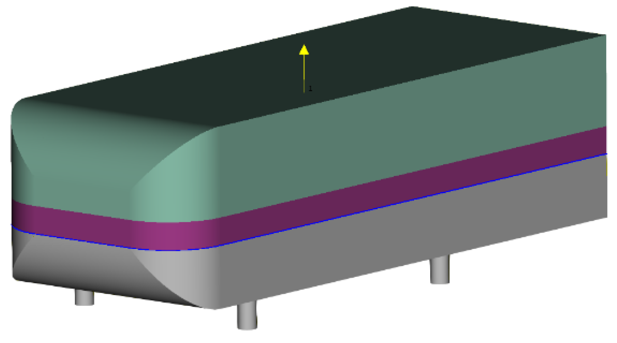
3.2. Simplified Geometry “S2A”

The surrogate model has been tested on a simplified industrial car design, which is used in the Renault wind tunnel facility for aerodynamic calibration. This design has the essential structures of a real vehicle while having enough simplicity to reduce computational complexity. It is made of multiple detailed structures: a superstructure, an underbody, front and rear axles, tires, and rims. The vehicle geometry is simplified with no external appendices (such as external mirrors) or engine compartments. Parametrization of the car shape involves three independent parameters, i.e., $\mathit{\mu }=({\mu }_1,{\mu }_2,{\mu }_3)$, affecting only the vehicle body superstructure. The first parameter ${\mu }_1$ corresponds to a translation along the $\widehat{\mathit{y}}$ axis, simulating a narrowing of the rear bumper and constrained within the range of $[-20\mathrm{mm},20\mathrm{mm}]$. The second parameter ${\mu }_2$ represents a translation along the $\widehat{\mathit{x}}$ axis to model an extension of the vehicle’s roof, with a range of $[-50\mathrm{mm},50\mathrm{mm}]$. Lastly, the third parameter ${\mu }_3$ denotes a rotation around the $\widehat{\mathit{y}}$ axis of the rear underbody, constrained within $[-5^{\circ },5^{\circ }]$. The specific morphing area impacted by these parameters is illustrated in Figure 3. The initial geometry is represented by an FE mesh composed of $N_v$ = 556,354 nodes.

Figure 3. Presentation of the S2A geometry involving three independent parameters. The variable surface part of the geometry is drawn in magenta.

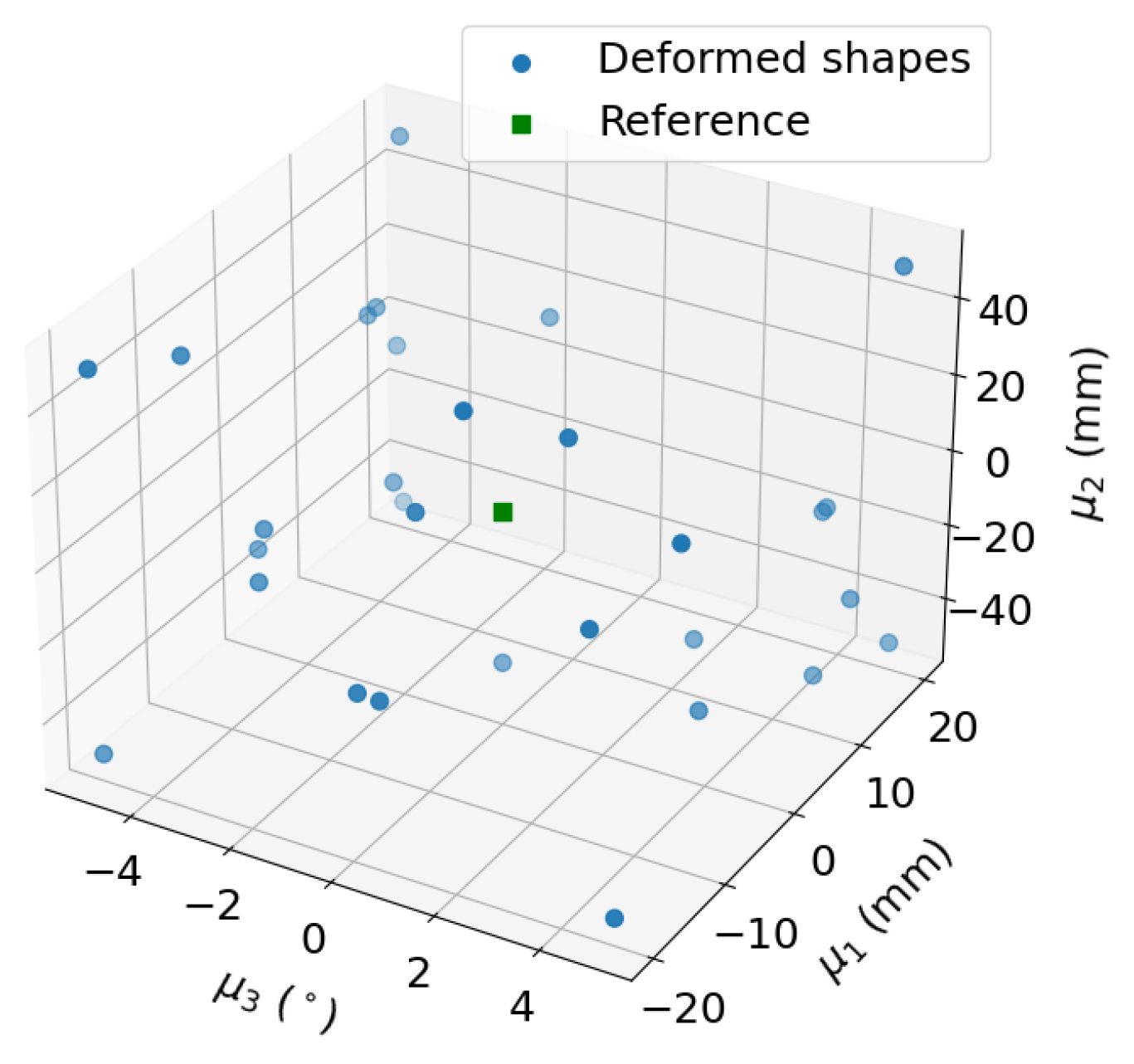
3.3. Data Generation and Preprocessing

A total of 30 deformed shapes are generated from the initial geometry, employing a maximin space-filling strategy on the CAD parameter $\mathit{\mu }$ (Figure 4). CFD simulations are performed for each shape, and the high-fidelity results provide detailed information on the flow field around the vehicles and the corresponding drag coefficients (Table 1). The mean dimensionless surface drag of this dataset is $0.9952$ with a standard deviation of $0.0127$. The low standard deviation, compared to the mean, suggests that the drag coefficients are relatively consistent across the dataset since shape variations are within a maximum range of 50 mm. However, in a design optimization study, even a small reduction in drag of $0.02$ $m^2$ is important as it could lead to a reduction of 1 g of ${\mathrm{CO}}_2$ consumption when proceeding to the Worldwide Harmonized Light Vehicles Test Procedure (WLTP) cycle.

Figure 4. Maximin space-filling on CAD parameter $\mathit{\mu }\in {\mathbb{R}}^3$.

Table 1. Table of dimensionless drag results (the surface drag of the reference shape is 1). The range is $[0.9632,1.0168]$.

Shape ID	$\frac{{\mathit{C}}_{\mathit{d}}\mathit{A}}{{\mathit{C}}_{\mathit{d}}{\mathit{A}}^{\mathit{ref}}}$	Set	Shape ID	$\frac{{\mathit{C}}_{\mathit{d}}\mathit{A}}{{\mathit{C}}_{\mathit{d}}{\mathit{A}}^{\mathit{ref}}}$	Set
1	1.0000	Reference	17	1.0075	Training
2	0.9820	Validation	18	0.9974	Validation
3	0.9939	Validation	19	1.0168	Training
4	0.9836	Validation	20	0.9632	Training
5	1.0011	Validation	21	0.9616	Training
6	1.0046	Validation	22	0.9987	Validation
7	0.9994	Validation	23	0.9761	Validation
8	0.9831	Validation	24	0.9790	Validation
9	1.0088	Validation	25	0.9952	Validation
10	0.9921	Validation	26	0.9858	Validation
11	1.0054	Validation	27	0.9712	Validation
12	0.9844	Validation	28	0.9943	Validation
13	0.9785	Validation	29	1.0101	Validation
14	0.9955	Validation	30	1.0043	Validation
15	0.9969	Validation	31	0.9775	Validation
16	1.0100	Validation

In this test case, each deformed geometry is independently meshed; therefore, the meshes do not share the same mesh topology as the reference shape. As explained in Appendix A, an optimal transport strategy is used to make the mapping and mesh correspondence. The optimal transport problem was solved by using the reference open-source Python library Geomloss [34].

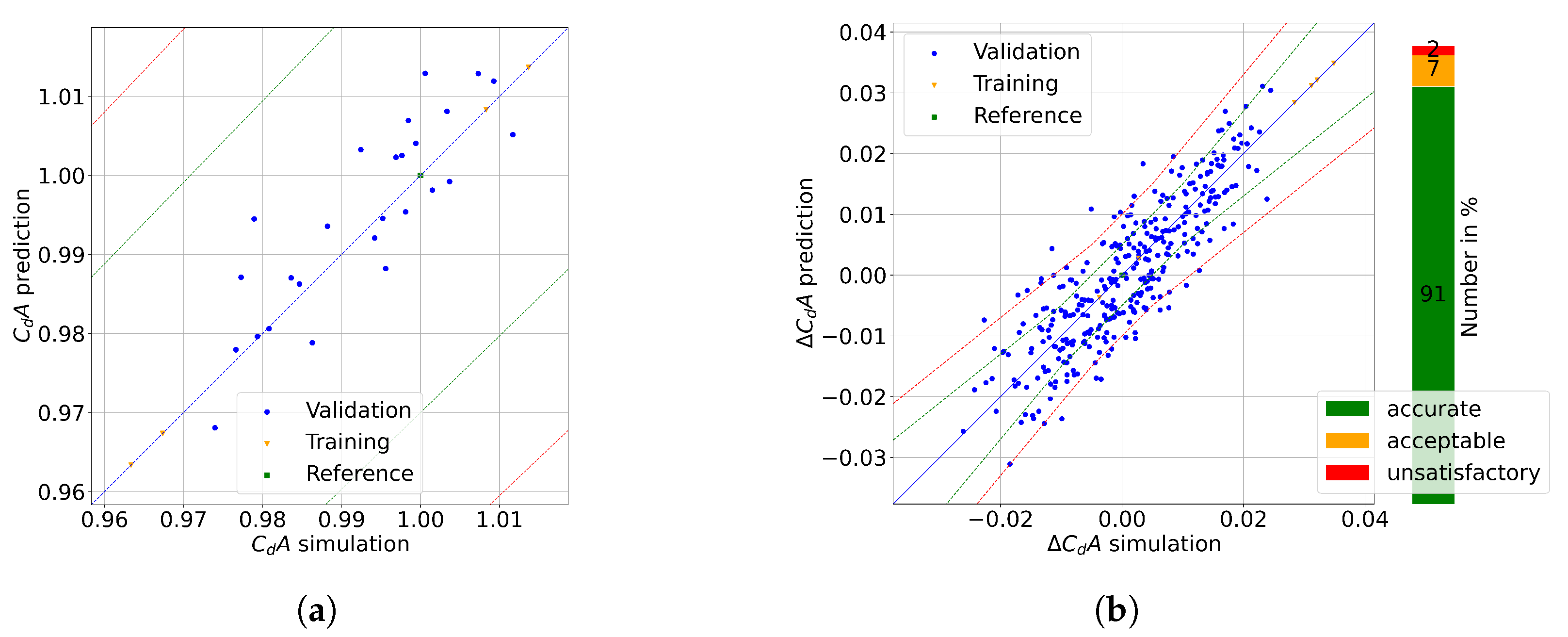
3.4. Model Performance

The performance of the model with respect to the number of input data points and their distribution is evaluated. To achieve this, cross-validation is performed using different numbers of folds. The number of folds, denoted by $N_f$, determines how the data is split for training and validation. The dataset is divided into $N_f$ subsets of approximately equal size. Usually in cross-validation, for each round, one subset is used for validation while the remaining $N_f-1$ subsets are used for training. However, in this study, as we aim to keep a low number of training data, the typical approach is reversed: one fold is used for training and the remaining folds are used for validation. This allows us to assess how well the model performs when it is trained on a small dataset. To ensure robustness of cross-validation results, multiple cross-validation runs are performed for each choice of fold number $N_f$. In each run, a different random seed is used to shuffle the data, resulting in different splits. This is performed to minimize the impact of any particular split that may be suboptimal for the model. After performing these cross-validation runs, the results are averaged to provide an estimate of the model’s performance. This approach is especially important when the number of folds is small, as the randomness in splitting the data can sometimes lead to unfavorable training datasets, potentially leading to misleading performance evaluations. By repeating the process with different splits, the model’s evaluation becomes more accurate and less dependent on any single data split.

Cross-validation is performed with the number of folds $N_f$ varying between 2 and 8. This results in training subsets containing between 15 samples (for $N_f=15$) and 3 or 4 samples (for $N_f=8$). For each number of folds, a total of 10 cross-validation runs are executed.

First, the performance of the low-dimensional reparametrization of the vehicle geometry is evaluated for each cross-validation fold. To do so, the Mean Squared Error (MSE), interpreted here as the $L^2$ projection error, is computed for each shape in the validation datasets. This error measures how well the geometry of the vehicle is reconstructed from the reduced parameter space. The MSE is then averaged across all validation shapes for each fold. As shown in Figure 5, the average MSE tends to increase as the number of folds increases as there are less data for training. However, the MSE values remain relatively low (less than $0.5$ mm), even with a high number of folds. This demonstrates the effectiveness of the reparametrization in capturing the geometric variations in the vehicle shapes, even with limited training data.

Figure 5. Averaged Mean Squared Error of shape reconstruction depending on the number of folds in cross-validation.

Then, to evaluate the performance of the model in predicting the drag coefficient for new shapes, several metrics are computed during cross-validation. First, the maximal and mean absolute error on $C_{d}A$ prediction are assessed. Figure 6a shows the results for the different folds. Although the error tends to increase slightly with the number of folds, the overall error remains well within an acceptable threshold of 3%, indicating the robust performance of the model with limited input data. The Pearson coefficient is computed to quantify the linear correlation between the predicted and high-fidelity drag values (Figure 6b). The model consistently achieved high Pearson correlation coefficients across all folds. Since the model is intended to serve as a decision support tool during the design optimization process, it is important that the ranking of shapes regarding drag is preserved. The model’s ability to maintain the correct ranking is then evaluated using the Kendall rank correlation coefficient [35]. The Kendall coefficient is defined by the following equation [36]:

$$\tau ={\displaystyle \frac{n_c-n_d}{n}},$$

(18)

with $n_c$ being the number of concordant pairs, $n_d$ the number of discordant pairs, and n the total number of pairs. A concordant pair is a pair of observations wherein the predicted and high-fidelity values have the same relative ordering. So, if one shape has a higher predicted drag value than another, and the actual drag values follow the same order, the pair is considered concordant. On the other hand, a discordant pair is when the relative ordering is not preserved by the prediction. However, this definition of discordant pairs can be too strict for aerodynamic studies. In some cases, pairs are considered discordant when the predicted and actual rankings are inverted, even though the difference in drag values between the configurations is very small. In such cases, the small deltas may not significantly affect the overall ranking for design studies. Therefore, it would be more appropriate to classify these pairs as concordant. A relaxed methodology is introduced to take this threshold into account. It introduces a threshold to account for minor prediction errors, allowing pairs with a small simulated delta to remain concordant if the predicted delta is similarly close. For larger differences in drag, a more relaxed threshold is used. In the following analysis, two variants of the relaxed Kendall coefficient are used to assess the model ranking performance with different tolerance levels. The first tolerance level allows a higher margin of error in the drag prediction, representing the maximum value for the prediction to be considered acceptable. The second tolerance level is stricter, requiring a smaller margin of error to classify the prediction as accurate. These two variants will be referred to as Relaxed Kendall Acceptable and Relaxed Kendall Accurate. The tolerance for the Relaxed Kendall Acceptable coefficient is defined as follows:

$$threshol{d}_{acceptable}=\left\{\begin{array}{cc}|\Delta C_{d}A|+{\displaystyle \frac{|\Delta C_{d}A|}{5}}+0.009\hfill & \mathrm{if}|\Delta C_{d}A|>0.005\hfill \\ |\Delta C_{d}A|+0.01\hfill & \mathrm{otherwise}\hfill \end{array}\right.$$

(19)

The tolerance for the Relaxed Kendall Accurate coefficient is defined as follows:

$$threshol{d}_{accurate}=\left\{\begin{array}{cc}|\Delta C_{d}A|+{\displaystyle \frac{|\Delta C_{d}A|}{5}}+0.003\hfill & \mathrm{if}\Delta |C_{d}A|>0.01\hfill \\ |\Delta C_{d}A|+0.005\hfill & \mathrm{otherwise}\hfill \end{array}\right.$$

(20)

where $|\Delta C_{d}A|$ is the absolute drag difference between two configurations. A predicted drag difference $\widetilde{\Delta C_{d}A}$ is classified as concordant if it is the same sign as $\Delta C{d}_A$ or if one of the following apply:

Figure 6. (a) Mean and max absolute relative error on $C_{d}A$ depending on the number of folds for cross-validation. (b) Correlation scores depending on the number of folds for cross-validation.

• $|\widetilde{\Delta C_{d}A}|\le threshol{d}_{accurate}$ for the Relaxed Kendall Accurate coefficient;
• $|\widetilde{\Delta C_{d}A}|\le threshol{d}_{acceptable}$ for the Relaxed Kendall Acceptable coefficient.

The values of the Kendall coefficients depending on the number of folds are presented in Figure 6b. The Kendall rank coefficient computed across all folds is in the range of 0.575 to 0.59. This low value is due to many pairs being classified as discordant with the strict initial definition of concordance and discordance. However, when the Relaxed Kendall is applied, using the modified definitions that account for minor prediction errors, a significant improvement in the score is observed. Indeed, across all folds, the Relaxed Kendall Acceptable and Relaxed Kendall Accurate coefficients are in a respective range of 0.93 to 0.94 and 0.86 to 0.89.

The total time of the modeling process is measured, including the three main phases: data preprocessing, model training, and inference. The preprocessing of the data consists in mesh correspondence by using optimal transport. During this step, the computational time mainly depends on the number of triangular elements representing the shape. This step can be skipped if the mesh is morphed simultaneously with the geometry. When using the Geomloss library, optimal transport for a shape with $N_v$ = 556,354 elements takes approximately 15 min on a system with 40 CPUs. The training time depends on the number of input samples, which is linked to the number of folds in cross-validation. Figure 7 illustrates how the training time varies with different numbers of folds. As the number of folds increases, the training time decreases because the model becomes easier to solve with fewer data points in each training subset. The training of the model with 15 shapes (two folds) takes approximately 10 s, while the training time drops to under 5 s when only 3–4 shapes (eight folds) are used in the training set. For the inference of a new shape, once the new geometry is generated using a morphing tool, no additional preprocessing via optimal transport is required if the mesh shares the same topology as the reference shape. In this case, the inference time is extremely short, taking less than 1 s to obtain the results on the cutting plane and the drag force.

Figure 7. Training and inference time depending on the number of folds for cross-validation.

The cross-validation experiment demonstrated that, with a small number of folds, resulting in a large amount of input data, the performance of the model increases. However, even with limited training data, the performance of the model is relatively high. Therefore, it is advantageous to work with the smallest number of input data points, as this reduces the number of CFD simulations required.

3.5. Surrogate Model Construction

When working with a small input dataset, the choice of training input data is very important to achieve good accuracy. Therefore, in the following analysis, four deformed shapes are chosen wisely (ID numbers 17, 19, 20, and 21 in Table 1) to train the model. The $N_s=4$ input samples are selected to ensure minimal comprehensive coverage of the exploration space of global parameters $\mathit{\mu }$. Additionally, the initial reference shape (shape ID 1) is included for computation of the shape variations. All the other shapes in the dataset serve as the validation set. The distribution of the selected shapes can be seen in Figure 8.

Figure 8. Maximin space-filling on CAD parameter $\mathit{\mu }\in {\mathbb{R}}^3$. Orange dots are the $N_s=4$ training shapes, the green dot is the reference geometry $\mathit{\mu }=\mathbf{0}$, and the remaining blue dots are used for the validation set.

3.5.1. Shape Encoding

Once the mesh mapping is complete, shape variation fields ${\mathit{\delta }}_{\mu }\in {\mathbb{R}}^{3N_v}$ of the training geometries are used as the shape variation basis. The norm of the deformation field is shown in Figure 9 and Figure 10, for two shapes of the training set. The training shapes cover both positive and negative deformations for parameters ${\mu }_1$, ${\mu }_2$, and ${\mu }_3$, ensuring a faithful representation of the exploration space.

Figure 9. Shape deformation field norm for training shape ID number 19.

Figure 10. Shape deformation field norm for training shape ID number 21.

The field of ${\mathit{\delta }}_{\mu }$ is used to compute the new shape basis ${\mathit{q}}_{\ell }$ and resulting shape coefficients $\mathit{\nu }\left(\mathit{\mu }\right)$. The relative $L^2$ error projection on the given basis is plotted in Figure 11 for the validation shapes. The overall error is quite small, with a maximum error of $0.002$ m for all shapes in the validation database.

Figure 11. Relative $L^2$ error projection on the ${\mathit{q}}_{\ell }$ POD basis for each shape of the database.

This new basis enables good reconstruction of the shape, indicating that it effectively captures the essential features and variations present in the original data.

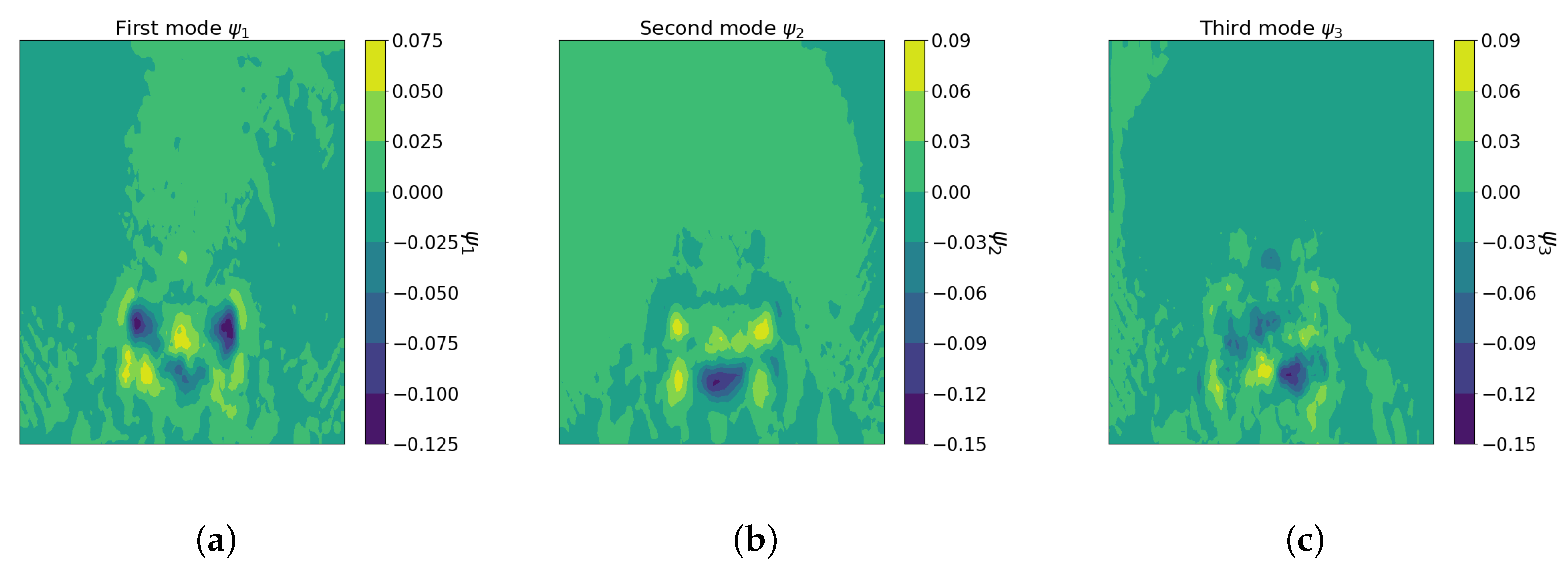
3.5.2. Computation of the Flow Field Modes on a Wake Cutting Plane

The snapshot matrix U of $\Delta \kappa$ fields is built from the FOM results. These results are obtained on a cutting plane located at a distance of $0.2\mathrm{m}$ behind the car (Figure 12a), discretized with $N_{cp}=6930$ nodes. It is worth noting that the flow on a wake plane close to the vehicle is turbulent with large unsteady eddies and lacks the stabilization observed in planes situated farther away. Therefore, the influence of shape variations becomes more pronounced and discriminating on proximity planes, providing valuable insights on the aerodynamic behavior of the vehicle. As shown in Figure 12b–d, the flow fields for the training shapes have different turbulent patterns. This difference will allow the model to learn a broader range of physical behavior to enhance its generalization ability for better predictive performance.

Figure 12. Flow field on cutting plane located $0.2$ m from the vehicle. (a) Cutting planes of study in the wake at respective locations $0.2$ m and $3.2$ m from the vehicle. (b) Delta fields $\Delta \mathit{\kappa }\left(\mathit{\mu }\right)$ for shape ID 17 on the wake plane located $0.2$ m from the vehicle. (c) Delta fields $\Delta \mathit{\kappa }\left(\mathit{\mu }\right)$ for shape ID 19 on the wake plane located $0.2$ m from the vehicle. (d) Delta fields $\Delta \mathit{\kappa }\left(\mathit{\mu }\right)$ for shape ID 20 on the wake plane located $0.2$ m from the vehicle.

Far-field modes, denoted as ${\mathit{\psi }}_1$, ${\mathit{\psi }}_2$, ${\mathit{\psi }}_3$, and ${\mathit{\psi }}_4$, are computed and depicted in Figure 13. Unlike Principal Component Analysis (PCA), the first mode resulting from the QR decomposition of U is not a linear combination of the columns of matrix U. This initial mode is the normalized first column of matrix U, as illustrated in Figure 13a. Then, each additional mode is orthogonal to the previous ones, so it captures distinct and independent flow field dynamics. With this approach, each mode provides new insights on the pattern of flow behavior.

Figure 13. Modes on cutting plane $S_{cp}$. (a) Contour plot of far-field mode ${\mathit{\psi }}_1$. (b) Contour plot of far-field mode ${\mathit{\psi }}_2$. (c) Contour plot of far-field mode ${\mathit{\psi }}_3$.

3.6. Surrogate Model Evaluation

Once the reparametrization has been completed and the physical modes are computed, the constant coefficient matrix A is determined, which concludes the model training on the $N_s=4$ shapes. The model is then applied to predict the density force $\mathit{\kappa }\left(\mathit{\mu }\right)$ on the cutting plane for the deformed shapes in the validation dataset. Figure 14 compares the flow field from the high-fidelity simulation with the predicted one from the surrogate model for one arbitrary shape from the validation set (Shape ID 7). The model successfully captures the overall flow patterns, confirming that the surrogate model accurately represents the fluid behavior. However, as shown in Figure 14c, errors are observed in some turbulent regions, where the model struggles to capture finer details.

Figure 14. Prediction results of the flow field. (a) Simulated flow field. (b) Predicted flow field. (c) Absolute relative error.

The MSE of the flow field predictions is given in Figure 15 for the different shapes of the validation dataset. The MSE value is relatively low for all configurations, with an average MSE of 0.38, indicating the strong overall predictive performance of the model.

Figure 15. Mean Squared Error of the flow field predictions for various shapes in the validation dataset.

The predicted flow field density $\mathit{\kappa }\left(\mathit{\mu }\right)$ is integrated over the cutting plane by the mean of Equation (17) to obtain the drag coefficient of each deformed shape. The accuracy of the surrogate model is assessed by comparing the predicted drag coefficient against those obtained from FOM results. As shown by the correlation plot in Figure 16a, there is a strong positive correlation between predicted and real drag coefficients, with a Pearson coefficient of 0.86. All predicted coefficients lie in the admissible threshold error range of 0–3% (green dotted line), with a maximal error of 1.59%. However, it is important to note that the order is not perfectly preserved for some geometries, indicating that the model captures the overall trend but may struggle with specific variations. To further examine these nuanced behaviors at particular points, the correlation plot of delta drag between each configuration is presented in Figure 16b. This plot reveals a positive correlation between predicted and real deltas. Most points are located within the threshold for acceptable (red dotted line) and accurate (green dotted line) prediction. More than 91% of deltas between configurations are predicted accurately, with only 2% of predictions falling outside the acceptable range. Moreover, the associated Kendall coefficients for this model are as follows: 0.67 for the standard Kendall coefficient, 0.95 for the Relaxed Kendall Accurate, and 0.99 for the Relaxed Kendall Acceptable. These different results demonstrate the model’s excellent effectiveness in predicting drag coefficient variations.

Figure 16. Prediction results. (a) Correlation plot of $C_{d}A$. (b) Correlation plot of delta of $\Delta C_{d}A$ and its distribution.

4. Concluding Remarks and Perspectives

In this paper, we presented a novel ML-based surrogate model for predicting drag forces on shape-parametrized cars, addressing the constraints of limited high-fidelity CFD simulations. The model features low-dimensional reparametrization of vehicle geometry, integration of physical fields to enhance data information without extra CFD computations, reliance on physical drag formulas, and accuracy for small geometry variations.

The surrogate model showed robust predictive capabilities across various 3D deformed geometries, enabling rapid assessment of minor shape variations during optimization. The model achieves typical mean square errors of order 2% for drag prediction with only few evaluations. While occasional challenges in preserving variation order were noted, the consistently low maximal error underscores its reliability for decision support and optimization studies.

Future work aims to enhance the model by incorporating more physical field modes and exploring different deformation fields for reparametrization. Additionally, refining the Design of Experiment selection could further optimize the methodology.

Appendix A.1

If the initial geometry $\underline{S}(.,{\mathit{\mu }}^{ref})$ and the deformed geometry $\underline{S}(.,\mathit{\mu })$ do not share the same mesh topology, as in the case of remeshing, establishing a correspondence between the two meshes is necessary. One approach to achieve this is to employ optimal transport between the nodes or elements of the two meshes. In this context, the initial geometry $\underline{S}(.,{\mathit{\mu }}^{ref})$ and the deformed one $\underline{S}(.,\mathit{\mu })$ are treated as point clouds of element centroids, each consisting of $N_v$ and $N_v^{\mu }$ points, respectively. The centroids are noted as ${\left({\mathit{c}}_j\right)}_{j=1\dots M}$ for $\underline{S}(.,{\mathit{\mu }}^{ref})$ and ${\left({\mathit{c}}_i^{\mu }\right)}_{i=1\dots M^{\mu }}$ for $\underline{S}(.,\mathit{\mu })$, with each point assigned a mass $m_j$ and $m_i^{\mu }$, respectively. By default, point clouds are conceptualized as distributions of uniform mass, where $m_j={\displaystyle \frac{1}{M}}$ and $m_i^{\mu }={\displaystyle \frac{1}{M^{\mu }}}$.

The transport plan ${\mathit{\pi }}^{\mathit{\mu }}$ between $\underline{S}(.,\mathit{\mu })$ and $\underline{S}(.,{\mathit{\mu }}^{ref})$ is a matrix of dimensions $M^{\mu }\times M$, where $m_{ij}$ represents the amount of mass transported from the initial point ${\mathit{c}}_i^{\mu }\in \underline{S}(.,\mathit{\mu })$ to ${\mathit{c}}_j\in \underline{S}(.,{\mathit{\mu }}^{ref})$ (see Figure A1). The definition of the transport plan is formulated to minimize a transport cost, which is given by

$$\mathrm{cost}\left({\mathit{\pi }}^{\mathit{\mu }}\right)=\sum _{ij}{m}_{ij}\left|\right|{\mathit{c}}_j-{\mathit{c}}_i^{\mu }{\left|\right|}^2$$

(A1)

Therefore, each point ${\mathit{c}}_j\in \underline{S}(.,{\mathit{\mu }}^{ref})$ is connected to one or multiple points ${\mathit{c}}_i^{\mu }\in \underline{S}(.,{\mathit{\mu }}^{ref})$ with a specified weight $m_{ij}$ if $m_{ij}>0$.

Figure A1. Transport plan towards a reference point ${\mathit{c}}_j$ of the reference cloud. $m_{ij}$ represents the mass transport from point ${\mathit{c}}_i^{\mu }$ to point ${\mathit{c}}_j$.

References

- Lions, J.L.; Magenes, E. Non-Homogeneous Boundary Value Problems and Applications; Springer: Berlin/Heidelberg, Germany, 1972. [Google Scholar]
- Pironneau, O. On optimum design in fluid mechanics. J. Fluid Mech. 1974, 64, 97–110. [Google Scholar] [CrossRef]
- Jameson, A. Aerodynamic design via control theory. J. Sci. Comput. 1988, 3, 233–260. [Google Scholar] [CrossRef]
- Jameson, A. Optimum aerodynamic design using CFD and control theory, AIAA paper 95-1729. In Proceedings of the AIAA 12th Computational Fluid Dynamics Conference, San Diego, CA, USA, 19–22 June 1995. [Google Scholar]
- Cheylan, I.; Fritz, G.; Ricot, D.; Sagaut, P. Shape Optimization Using the Adjoint Lattice Boltzmann Method for Aerodynamic Applications. AIAA J. 2019, 57, 1–16. [Google Scholar] [CrossRef]
- Hardy, R.L. Multiquadric equations of topography and other irregular surfaces. J. Geophys. Res. 1971, 76, 1905–1915. [Google Scholar] [CrossRef]
- Buhmann, M.D. Radial Basis Functions: Theory and Implementation; Cambridge University Press: New York, NY, USA, 2003. [Google Scholar]
- MacKay, D.J.C. Introduction to Gaussian processes. NATO ASI Ser. F Comput. Syst. Sci. 1998, 168, 133–166. [Google Scholar]
- Brunton, S.L.; Bernd, R.N.; Koumoutsakos, P. Machine learning for fluid mechanics. Annu. Rev. Fluid Mech. 2020, 52, 477–508. [Google Scholar] [CrossRef]
- Pearson, K. On Lines and Planes of Closest Fit to Systems of Points in Space. Philos. Mag. 1901, 2, 559–572. [Google Scholar] [CrossRef]
- Lumley, J. Stochastic Tools in Turbulence; Academic Press: New York, NY, USA, 1970. [Google Scholar]
- Roweis, S.T.; Saul, L.K. Nonlinear Dimensionality Reduction by Locally Linear Embedding. Science 2000, 290, 2323–2326. [Google Scholar] [CrossRef]
- Umetani, N.; Bickel, B. Learning three-dimensional flow for interactive aerodynamic design. ACM Trans. Graph. 2018, 37, 1–10. [Google Scholar] [CrossRef]
- Li, X.; Xie, C.; Sha, Z. Part-Aware Product Design Agent Using Deep Generative Network and Local Linear Embedding. In Proceedings of the Hawaii International Conference on System Sciences, Kauai, HI, USA, 5–8 January 2021. [Google Scholar]
- Badías, A.; Curtit, S.; González, D.; Alfaro, I.; Chinesta, F.; Cueto, E. An augmented reality platform for interactive aerodynamic design and analysis. Int. J. Numer. Methods Eng. 2019, 120, 125–138. [Google Scholar] [CrossRef]
- Song, B.; Yuan, C.; Permenter, F.; Arechiga, N.; Ahmed, F. Surrogate Modeling of Car Drag Coefficient with Depth and Normal Renderings. In Proceedings of the ASME 2023 International Design Engineering Technical Conferences and Computers and Information in Engineering Conference, Volume 3A: 49th Design Automation Conference (DAC), Boston, MA, USA, 20–23 August 2023. [Google Scholar]
- Xie, S.; Girshick, R.; Dollar, P.; Tu, Z.; He, K. Aggregated Residual Transformations for Deep Neural Networks. In Proceedings of the 30th IEEE Conference on Computer Vision and Pattern Recognition, Honolulu, HI, USA, 21–26 July 2017; pp. 5987–5995. [Google Scholar]
- Rosset, N.; Cordonnier, G.; Duvigneau, R.; Bousseau, A. Interactive design of 2D car profiles with aerodynamic feedback. Comput. Graph. Forum 2023, 42, 427–437. [Google Scholar] [CrossRef]
- Guo, X.; Li, W.; Iorio, F. Convolutional Neural Networks for Steady Flow Approximation. In Proceedings of the 22nd ACM SIGKDD International Conference on Knowledge Discovery and Data Mining Association for Computing Machinery, New York, NY, USA, 13–17 August 2016; pp. 481–490. [Google Scholar]
- Jacob, S.; Mrosek, M.; Othmer, C.; Köstler, H. Deep Learning for Real-Time Aerodynamic Evaluations of Arbitrary Vehicle Shapes. SAE Int. J. Passeng. Veh. Syst. 2022, 15, 77–90. [Google Scholar] [CrossRef]
- Ronneberger, O.; Fischer, P.; Brox, T. U-Net: Convolutional Networks for Biomedical Image Segmentation. Med Image Comput.-Comput.-Assist. Interv. 2015, 9351, 234–241. [Google Scholar]
- Heft, A.; Indinger, T.; Adams, N. Introduction of a New Realistic Generic Car Model for Aerodynamic Investigation. SAE Tech. Pape 2012-01-0168 2012. [Google Scholar]
- Monti, F.; Boscaini, D.; Masci, J.; Rodola, E.; Svoboda, J.; Bronstein, M.M. Geometric Deep Learning on Graphs and Manifolds Using Mixture Model CNNs. In Proceedings of the 30th IEEE Conference on Computer Vision and Pattern Recognition, Honolulu, HI, USA, 21–26 July 2017; pp. 5115–5124. [Google Scholar]
- Baqué, P.; Remelli, E.; Fleuret, F.; Fua, P. Geodesic Convolutional Shape Optimization. In Proceedings of the 35th ICML, Stockholm, Sweden, 10–15 July 2018; pp. 481–490. [Google Scholar]
- Durasov, N.; Lukoyanov, A.; Donier, J.; Fua, P. DEBOSH: Deep Bayesian Shape Optimization. arXiv 2021, arXiv:2109.13337. [Google Scholar]
- Remelli, E.; Lukoianov, A.; Richter, S.R.; Guillard, B.; Bagautdinov, T.; Baque, P.; Fua, P. MeshSDF: Differentiable Iso-Surface Extraction. Adv. Neural Inf. Process. Syst. 2020, 33, 22468–22478. [Google Scholar]
- Gunpinar, E.; Coskun, U.C.; Ozsipahi, M.; Gunpinar, S. A Generative Design and Drag Coefficient Prediction System for Sedan Car Side Silhouettes based on Computational Fluid Dynamics. Comput.-Aided Des. 2019, 111, 1–10. [Google Scholar] [CrossRef]
- Ando, K.; Takamura, A.; Saito, I. Automotive aerodynamic design exploration employing new optimization methodology based on CFD. SAE Int. J. Passeng. Cars-Meek Syst. 2010, 3, 398–406. [Google Scholar] [CrossRef]
- Bertram, A.; Othmer, C.; Zimmermann, R. Towards Real-time Vehicle Aerodynamic Design via Multi-fidelity Data-driven Reduced Order Modeling. In Proceedings of the 2018 AIAA/ASCE/AHS/ASC Structures, Structural Dynamics, and Materials Conference, Kissimmee, FL, USA, 8–12 January 2018. [Google Scholar]
- Clancy, L.J. Aerodynamics; Wiley: Hoboken, NJ, USA, 1975. [Google Scholar]
- Anderson, J. Fundamentals of Aerodynamics, 6th ed.; McGraw-Hill: New York, NY, USA, 2016. [Google Scholar]
- Onorato, M.; Costelli, A.; Garrone, A. Drag Measurement Through Wake Analysis. SAE Tech. Pape. 840302 1984, 85–93. [Google Scholar]
- Sagaut, P. Large Eddy Simulation for Incompressible Flows; Springer: Berlin/Heidelberg, Germany, 2006. [Google Scholar]
- Feydy, J.; Séjourné, T.; Vialard, F.-X.; Amari, S.-I.; Trouve, A.; Peyré, G. Interpolating between Optimal Transport and MMD using Sinkhorn Divergences. In Proceedings of the 22nd International Conference on Artificial Intelligence and Statistics, Naha, Japan, 16–18 April 2019; pp. 2681–2690. [Google Scholar]
- Kendall, M.G. A new measure of rank correlation. Biometrika 1938, 30, 81–93. [Google Scholar] [CrossRef]
- Nelsen, R.B. Kendall tau metric. Encycl. Math. 2001, 3, 226–227. [Google Scholar]
Disclaimer/Publisher’s Note: The statements, opinions and data contained in all publications are solely those of the individual author(s) and contributor(s) and not of MDPI and/or the editor(s). MDPI and/or the editor(s) disclaim responsibility for any injury to people or property resulting from any ideas, methods, instructions or products referred to in the content. |
© 2024 by the authors. Licensee MDPI, Basel, Switzerland. This article is an open access article distributed under the terms and conditions of the Creative Commons Attribution (CC BY) license (https://creativecommons.org/licenses/by/4.0/).