G-TS-HRNN: Gaussian Takagi–Sugeno Hopfield Recurrent Neural Network

Abstract

The Hopfield Recurrent Neural Network (HRNN) is a single-point descent metaheuristic that uses a single potential solution to explore the search space of optimization problems, whose constraints and objective function are aggregated into a typical energy function. The initial point is usually randomly initialized, then moved by applying operators, characterizing the discrete dynamics of the HRNN, which modify its position or direction. Like all single-point metaheuristics, HRNN has certain drawbacks, such as being more likely to get stuck in local optima or miss global optima due to the use of a single point to explore the search space. Moreover, it is more sensitive to the initial point and operator, which can influence the quality and diversity of solutions. Moreover, it can have difficulty with dynamic or noisy environments, as it can lose track of the optimal region or be misled by random fluctuations. To overcome these shortcomings, this paper introduces a population-based fuzzy version of the HRNN, namely Gaussian Takagi–Sugeno Hopfield Recurrent Neural Network (G-TS-HRNN). For each neuron, the G-TS-HRNN associates an input fuzzy variable of d values, described by an appropriate Gaussian membership function that covers the universe of discourse. To build an instance of G-TS-HRNN(s) of size s, we generate s n-uplets of fuzzy values that present the premise of the Takagi–Sugeno system. The consequents are the differential equations governing the dynamics of the HRNN obtained by replacing each premise fuzzy value with the mean of different Gaussians. The steady points of all the rule premises are aggregated using the fuzzy center of gravity equation, considering the level of activity of each rule. G-TS-HRNN is used to solve the random optimization method based on the support vector model. Compared with HRNN, G-TS-HRNN performs better on well-known data sets.

1. Introduction

Preoccupations with computational accuracy, speed, and engineering completeness have prompted scientists to investigate soft computing approaches to modeling, forecasting, and monitoring nonlinear dynamic systems. Both artificial neural networks (ANNs) and fuzzy logic approaches are widely employed as techniques for soft computation. The marriage of such techniques is being applied in numerous areas of science and engineering to tackle real-world challenges, in particular, optimization problems. The utilization of fuzzy logic has the potential to enhance the ability of a machine learning system to reason and infer. Categorical insights, however vague, may be modeled to permit the symbolic articulation of automatic learning through fuzzy logic. The use of neural networks incorporates learning capability, robustness, and massive parallelism into the system. The representation of expert knowledge and the machine-learning capacities of the neuro-fuzzy network turn it into a potent framework to tackle automatic learning challenges [1,2]. Currently, training techniques and the architecture of traditional neuro-fuzzy nets have been refined to deliver higher levels of performance in terms of accuracy and learning time.

On the one hand, the Takagi–Sugeno–Kang (TSK) induction scheme is the leading fuzzy inference system and a powerful tool for building complex nonlinear dynamical systems. The main advantage of TSK modeling is its “multimodal” nature: it is able to merge nonlinear submodels to describe the global dynamics of a complex system [3]. On the other hand, the Hopfield Recurrent Neural Network (HRNN) is distinctive as a particular sort of recurrent neural network that has grown rapidly and gained significant interest among scientists in a range of fields, especially optimization [4,5,6,7,8]. This network has shown itself to be extremely efficient over other approaches, notably in delivering high-performance answers to mathematical optimization problems [9,10,11,12,13,14,15].

This paper introduces a population-based fuzzy version of the Hopfield recurrent neural network, namely the Gaussian Takagi–Sugeno Hopfield Recurrent Neural Network (G-TS-HRNN).

1.1. Hopfield Recurrent Neural Network: Main Knowledge

The HRNN is a semantically recurrent neural network consisting of a monolayer of n units that are completely interconnected, where each neuron has an activating function. This network is considered a driven system characterized using a dynamic equation specified as follows [9]:

$${\displaystyle \frac{du}{dt}}=Tv+I$$

(1)

In Equation (1), $T\in {\mathbb{R}}^{n\times n}$ represents the link strength of the neurons, $I\in {\mathbb{R}}^n$ is the bias, u is the state vector of different units, and v is the vector activations of the different units. The correlation that exists between the vector of states u and their activations v can be expressed by the activation function $v=g\left(u\right)$ (generally a hyperbolic tangent), limited at the lower end with 0 and higher end with 1 and has a soft threshold.

Definition 1.

A state vector $u^e$ is referred to as the equilibrium point of Equation (1) when, for a given entry vector $u^0$, $u^e$ fulfills the following conditions: $u\left(t\right)=u^e\forall t\ge t_e$ at some $t_e\ge 0$.

The $E_{Lyap}$ energy function can be employed to investigate the stability of HRNN. This function serves to demonstrate whether the network attains a steady state, as it must diminish as time goes by (${\displaystyle \frac{d{E}_{Lyap}}{dt}}\le 0$) in order for the system to tend towards a minimum. Such a Lyapunov function is expressible as shown below [9]:

$$E_{Lyap}\left(v\right)=-{\displaystyle \frac{1}{2}}{v}^{t}Tv-I^{t}v$$

(2)

The steady-state of the HRNN network would exist if the energy function exists. In 1984, Hopfield proved that if the matrix T is symmetric, then the energy function $E_{Lyap}$ holds.

The solution of optimization problems employing the HRNN usually requires the creation of an energy function. This function represents a mathematical description of the problem to be resolved [16]. The local minima of this energy function refers to the local optimal decision of the optimization problem [9,17,18]. If f and $g_j$, $\forall j=1,\dots ,m$, are the objective function and the set of constraints, respectively, of the optimization problem, a possible energy function can be defined as follows:

$$E\left(v\right)=\alpha f\left(v\right)+\sum _i{\varphi }_i{g}_i\left(v\right)+\sum _i{\varphi }_{i,j}{g}_i\left(v\right)g_j\left(v\right)$$

(3)

where $\alpha$, ${\varphi }_i$, and ${\varphi }_{i,j}$ are the penalty parameters used to control the amplitude of f and the violated constraints. The optimization of the E cost function requires appropriate parameters that guarantee the feasibility of the solutions. These parameters can be extracted in a suitable way on the basis of the first and second derivatives of the E function, using the hyperplane method, which prevents the system from reaching stability outside the feasible set delimited by the constraints of the optimization problem [9,12,13,15].

1.2. State of the Art

The Hopfield Recurrent Neural Network (HRNN) is widely used to solve Optimization Problems (OPs) based on the appropriate energy function. A local solution of the OP is obtained by solving the differential equation governing the dynamics of HRNN using numerical methods. This method falls within the descent approaches that consider only one individual at each iteration. Recall that the dynamics of HRNN is governed by the equation:

$${\displaystyle \frac{du\left(t\right)}{dt}}=Tv\left(t\right)+I,u\left(0\right)=u^0\in {\mathbb{R}}^n$$

(4)

where for a given $u_0>0$,

$$v_i\left(t\right)={\displaystyle \frac{e^{2u_i\left(t\right)u_0^{-1}}}{e^{2u_i\left(t\right)u_0^{-1}}+1}}\forall i=1,\dots ,n$$

To solve Equation (4), using the Euler–Cauchy method, each sub-equation is discretized using a time step called $\delta t$ [19]. This procedure implies a substantial local truncation error of the order of $O\left(\delta t^2\right)$ per pass, requiring the implementation of a very small step width at the expense of reduced speed and higher accuracy errors in floating-point calculations. It is also vulnerable to modifications of any scale [10]. In this way, the HRNN size, the magnitudes of weights, biases, and the gain parameter of the HRNN must be considered to assign the step size in the Euler method. In spite of all these objections, some authors have proposed a very small time step, which requires a lot of CPU time to obtain a local minimum and prevent the HRNN from escaping unpromising regions [20]. This is why some authors suggest increasing $\delta t$ to save computing time and explore more promising regions. For example, the authors of [21,22,23] believe that $\delta t\in [0.0001,0.01]$ is an accurate value in their calculation trials. However, with such a wide range of values, the trajectories can be irregular, skipping towards other attractors in the basin. This last property, however, can be used to improve solution quality by escaping from local minima, see Wang and Smith [24]. Given the increasing size of the HRNN, the Euler method and the Runge–Kutta method can be very slow in the search for a local optimum [11]. In [10], the authors introduce an algorithm with the optimal time step for HRNN to obtain an HRNN equilibrium point. This algorithm computes an optimal time-step in each iteration so that a rapid convergence to an equilibrium point is achieved. This technique has been widely used in real-world problems [12,14,15,25]. However, in the case of a non-quadratic objective function or constants, calculating the optimal time step becomes very difficult, requiring the use of fixed-point or Newton methods or quasi-Newton methods to estimate the optimal time step of the Euler–Cauchy algorithm [26,27,28]. However, calling several numerical functions at each iteration can make the search procedure very slow and does not guarantee convergence to a local solution.

Through these works, HRNN can be thought of as a single-point descent metaheuristic that uses a single potential solution to explore the search space. The point is usually randomly initialized and then moved by applying operators that modify its position or direction. Like all single-point metaheuristics, HRNN has certain drawbacks, such as being more likely to get stuck in local optima or miss global optima due to the use of a single point to explore the search space. In addition, it is more sensitive to the initial point and operator, which can influence the quality and diversity of solutions. Moreover, it can have difficulty with dynamic or noisy environments, as it can lose track of the optimal region or be misled by random fluctuations.

1.3. Contributions

To overcome the shortcomings discussed in Section 1.2, this paper introduces a fuzzy-neuro optimization method, namely Gaussian Takaji–Sugeno Hopfield Recurrent Neural Network (G-TS-HRNN). This is a population-based metaheuristic that has certain advantages over single-point metaheuristics, including classical HRNN.

To help classical HRNNs escape local optima while exploring promising regions of the search space, we have introduced a family of input fuzzy variables modeling variations in the quadratic factors of the system of Equation (4) governing the dynamics of HRNN. The initial HRNN stability point is approximated by fuzzy rules with linear differential equations as a consequence.

Sampling via the non-linear sector associated with the Takagi–Sugeno fuzzy model allows the initial HRNN to be decomposed into independent linear sub-problems, enabling parallel or distributed computing to speed up the search process and handle large-scale problems. Furthermore, to deal with the stochastic characteristics of real environments, we can strike an appropriate balance between exploration and exploitation when generating the fuzzy membership of Takaji–Sugeno fuzzy variables.

More precisely, to construct G-TS-HRNN, we associate a d-valued fuzzy input variable with each HRNN unit, described by an appropriate Gaussian membership function, that covers the universe of discourse determined by the slope of the HRNN neurons’ activation functions. To build an instance of G-TS-HRNN(s) of size s, we generate s n-uplets of fuzzy values that represent the premise of the Takagi–Sugeno system. The consequents are the differential equations governing the dynamics of the HRNN obtained by replacing each premise fuzzy value with the mean of different Gaussians. The steady points of all the rules consequents are aggregated using the fuzzy center of gravity equation, considering the level of activity of each rule. G-TS-HRNN is used to solve the random optimization method and solve the classification problem based on the support vector mathematical model. To ensure the feasibility of the decisions delivered by the considered models, we used the hyperplane technique introduced in [9] and used successfully in [12,15,25]. HRNN and G-TS-HRNN were tested on nine data sets found in the UCI (Machine Learning Repository) machine learning database [29]. The performance metrics considered in this work are accuracy, F1-measure, precision, and recall. Compared with the classical HRNN, G-TS-HRNN performs better on well-known data sets.

Towards the end, three choices need to be justified: (a) the nature of membership functions associated with the non-linear sector, (b) their number, and (c) their parameters. (a) Gaussian Mixture Models (GMMs) are considered universal approximators of densities, meaning they can approximate any smooth density function to an arbitrary degree of accuracy given a sufficient number of components [30]. This property makes GMMs highly versatile in modeling complex distributions in various fields, including statistics and machine learning [31]. (b) The choice of the number of Gaussians must strike a balance between exploration, diversification, and complexity of the G-TS-HRNN; in our case, this selection is made experimentally. (c) When designing membership functions for fuzzy variables, certain conditions must be satisfied to ensure system accuracy and coherence [32]. Membership functions must collectively cover the entire universe of discourse. Parameters must be chosen such that overlap between adjacent membership functions is essential to enable smooth transitions, while the principle of completeness ensures that sets that overlap at any point add up to a meaningful total, often 1 [33].

Outline: Section 2 introduces the sector nonlinearity of the Takagi–Sugeno fuzzy model. Section 3 presents the Gaussian Takagi–Sugeno model applied to the Hopfield Recurrent Neural Network (G-TS-HRNN). Section 4 discusses the application of G-TS-HRNN to the classification problem using Support Vector Machines (SVMs). Section 5 outlines the experimentation and implementation conditions. Finally, Section 6 provides conclusions and future directions.

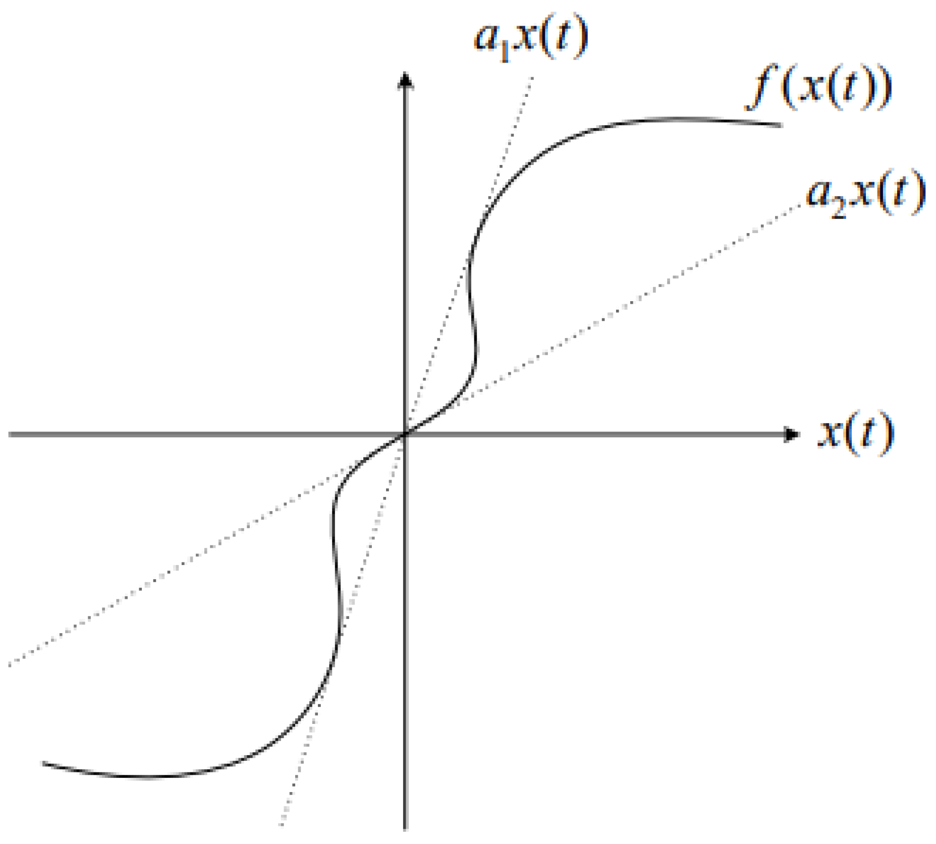
2. Sector Nonlinearity to Takagi–Sugeno Fuzzy Model

To build a Takagi–Sugeno pattern, we first have to design a T-S fuzzy map of a nonlinear model. Therefore, building a fuzzy model is an essential and fundamental task in this process. In general, two different strategies can be adopted to develop fuzzy models [34,35,36]: (a) identification (fuzzy modeling) based on entry-exit data, (b) deducing the governing equations of a specified non-linear operating system [37]. The recognition process of fuzzy modeling is tailored to plants that can or can not sufficiently be captured by analytical and/or physical models. In addition, nonlinear dynamic models for mechanical engineering systems may be simply derived, for instance, using the Lagrange and the Newton–Euler procedure. In such cases, the second approach, which derives a fuzzy model from given nonlinear dynamical models, is more appropriate. This brief review covers the second approach. This is an approach that employs the concept of “sectoral non-linearity”, “local approximation”, or a mixture of the two to generate fuzzy models.

Sector non-linearity revolves around the next idea. Take the following non-linear model:

$${\displaystyle \frac{dx\left(t\right)}{dt}}=f\left(x\right),x^0\in {\mathbb{R}}^n$$

(5)

where f is a non-linear function. The aim is to find the global sector such that

$${\displaystyle \frac{dx\left(t\right)}{dt}}=f\left(x\right)\in Ax\left(t\right),x^0\in {\mathbb{R}}^n$$

where A is a matrix free of x.

Figure 1 illustrates the sector nonlinearity approach in the case when $A=[a_1,a_2]$. This ensures the accurate building of the fuzzy model.

Suppose we can write Equation (5) as follows:

$${\displaystyle \frac{dx\left(t\right)}{dt}}=B\left(x\right)x\left(t\right),x^0\in {\mathbb{R}}^n$$

where $B\left(x\right)={\left(b_{ij}\left(x\right)\right)}_{i,j=1,\dots ,n}$ and $b_{ij}\left(x\right)\in [{\underline{b}}_{ij},{\overline{b}}_{ij}]$. Here, $b_{ij},i,j=1,\dots ,n$ are nonlinear terms in Equation (5), which represent the fuzzy variables that we name $z_{ij}$ and are called premise variables. The starting point in any fuzzy design is to establish the fuzzy variables and the fuzzy sets or membership functions. While there is no generic way of doing this, and it may be carried out by a number of methods, primarily trial-and-error, in precise fuzzy modeling using sectorial nonlinearity, it is entirely routine. In this tutorial, we assume that the premise variables are only functions of the state variables for reasons of simplicity [38].

To acquire membership functions, we should calculate the minimum and maximum values of $z_{ij}$, which are obtained as follows:

$min\left(z_{ij}\right)={\underline{b}}_{ij}$ and $max\left(z_{ij}\right)={\overline{b}}_{ij}$ Therefore, $z_{ij}$ can be represented by two membership functions $M_{ij}^{\left(1\right)}$ and $M_{ij}^{\left(2\right)}$ as follows: $z_{ij}={\underline{b}}_{ij}{M}_{ij}^{\left(1\right)}+{\overline{b}}_{ij}{M}_{ij}^{\left(2\right)},\forall i,j$ such that $M_{ij}^{\left(1\right)}+M_{ij}^{\left(2\right)}=1$. We associate $M_{ij}^{\left(1\right)}$ with the fuzzy value “Small” and $M_{ij}^{\left(2\right)}$ with the fuzzy value “Big”.

To each sample $s\in {\{Small,Big\}}^{n\times n}$, we introduce the following Takaji–Sugeno fuzzy rule:

If $z_{1,1}$ is $s_{1,1}$ and…$z_{n,n}$ is $s_{n,n}$, Then, ${\displaystyle \frac{dx\left(t\right)}{dt}}=B^{s}x\left(t\right),x^0\in {\mathbb{R}}^n$. where $B_{ij}^s={\underline{b}}_{ij}$ if $s_{ij}=Small$ else $B_{ij}^s={\overline{b}}_{ij}$ if $s_{ij}=Big$.

${\displaystyle \frac{dx\left(t\right)}{dt}}=B^{1}x\left(t\right),x\left(0\right)\in {\mathbb{R}}^n$.

${\displaystyle \frac{dx\left(t\right)}{dt}}=B^{2}x\left(t\right),x\left(0\right)\in {\mathbb{R}}^n$.

For a random $x^0\in {\mathbb{R}}^n$, to obtain an estimation x of the steady state of the system (5), we process it as follows:

(a) Generate k samples $s_1\in {\{Small,Big\}}^{n\times n},\dots ,s_k\in {\{Small,Big\}}^{n\times n}$;

(b) Calculate the steady state of the premises of the rules associated with these samples; let $x^{\left(1\right)},\dots ,x^{\left(k\right)}$ be these solutions obtained using the Euler–Cauchy method [9];

(c) Calculate the activation weight $w_s$ of a different rule for $s=1,\dots ,k$. As the elementary conditions of different rules are linked by the “and” operator, the $w_s=M_{1,1}^{\left(s\right)}\left(z_{1,1}^{\left(s\right)}\right)\wedge \dots \wedge M_{n,n}^{\left(s\right)}\left(z_{n,n}^{\left(s\right)}\right)$; where $z_{ij}^{\left(s\right)}=b_{ij}\left(x^{\left(s\right)}\right)$

(d) Use the fuzzy Center of gravity to estimate x: $x={\displaystyle \frac{{\sum }_{s=1}^k{w}_s{x}^{\left(s\right)}}{{\sum }_{s=1}^k{w}_s}}$.

3. Gaussian Takagi–Sugeno Hopfield Recurrent Neural Network (G-TS-HRNN)

Considering the equation of the activation function of the HRNN neurons (hyperbolic tangente tangent), the dynamical system (1) can also be expressed as:

$$\left\{\begin{array}{c}{\displaystyle \frac{d{v}_i}{dt}}={\displaystyle \frac{2}{u_0}}{v}_i(1-v_i)(\sum _{j=1}^n{T}_{ij}{v}_j+I_i),\forall i=1,\dots ,n\hfill \\ v_i\left(0\right)=v_i^0\in [0,1],\forall i=1,\dots ,n\hfill \end{array}\right.$$

(6)

To transform Equation (6) into a linear equation, we introduce n fuzzy sets defined on the following variables:

$$z_i={\displaystyle \frac{2}{u_0}}{v}_i(1-v_i),\forall i=1,\dots ,n$$

We have $min\left(z_i\right)=0$ and $max\left(z_i\right)={\displaystyle \frac{1}{u_0}}$; we set $U=m:s_0:M$ and $d=size\left(U\right)$, where $s_0={\displaystyle \frac{1}{p\ast u_0}}$ and p is a positive integer and $0\le m\le M\le {\displaystyle \frac{1}{u_0}}$. For each $z_i$, we introduce d fuzzy values $F_1,\dots ,F_d$ that we associate with d Gaussian $G_1(mean=m),\dots ,G_1(mean=m+l\ast s_0),\dots ,G_d(mean=m+(d-1)\ast s_0=M)$, respectively.

Example 1.

For $U={\displaystyle \frac{1}{10\ast u_0}}:{\displaystyle \frac{3}{10\ast u_0}}:{\displaystyle \frac{10}{10\ast u_0}}$, we have $d=4$ and we obtain the Gaussian membership functions shown in Figure 2 (obtained for a standard diviation of ${\displaystyle \frac{1}{7\ast u_0}}$). In this case, we can say that $F_1=Very\_Small$, $F_2=Small$, $F_3=Big$, and $F_4=Very\_Big$.

We pull N samples ${\pi }^1=(a_1^1,\cdots ,a_n^1),\cdots ,{\pi }^s=(a_1^s,\cdots ,a_n^s),\cdots ,{\pi }^N=(a_1^N,\cdots ,a_n^N)$ from $U^n$, where n is the number of neurons of a given HRNN. For each sample s, we denote by ${\pi }^s.a_i^s$ the fuzzy value associated with the Gaussian membership $G(\mathrm{mean}=a_i)$. We work with a Gaussian of the same standard deviation chosen to cover the universe of discourse.

Example 2.

We consider the same example as before and we pull the following five samples:

${\pi }^1=(a_1^1,\dots ,a_n^1)$,${\pi }^2=(a_1^2,\dots ,a_n^2)$, ${\pi }^3=(a_1^3,\dots ,a_n^3)$, ${\pi }^4=(a_1^4,\dots ,a_n^4)$, ${\pi }^5=(a_1^5,\dots ,a_n^5)$. If, in addition, the considered HRNN contains three neurons, we can express our sample as follows:

${\pi }^1=({\displaystyle \frac{4}{10\ast u_0}},{\displaystyle \frac{1}{10\ast u_0}},{\displaystyle \frac{7}{10\ast u_0}})$,${\pi }^2=({\displaystyle \frac{4}{10\ast u_0}},{\displaystyle \frac{4}{10\ast u_0}},{\displaystyle \frac{4}{10\ast u_0}})$, ${\pi }^3=({\displaystyle \frac{7}{10\ast u_0}},{\displaystyle \frac{10}{10\ast u_0}},{\displaystyle \frac{7}{10\ast u_0}}))$,

${\pi }^4=({\displaystyle \frac{1}{10\ast u_0}},{\displaystyle \frac{4}{10\ast u_0}},{\displaystyle \frac{7}{10\ast u_0}}))$, ${\pi }^5=({\displaystyle \frac{7}{10\ast u_0}},{\displaystyle \frac{7}{10\ast u_0}},{\displaystyle \frac{10}{10\ast u_0}}))$.

For each sample ${\pi }^s=(a_1^s,\dots ,a_n^s)$, we introduce the following rule $R\left({\pi }^s\right)$:

if $z_1$ is ${\pi }^s.a_1^s$ and $z_i$ is ${\pi }^s.a_i^s$ and … and $z_n$ is ${\pi }^s.a_n^s$,

then $\left\{\begin{array}{c}{\displaystyle \frac{d{v}_i}{dt}}=a_i^s({\sum }_{i=1}^n{T}_{ij}{v}_i+I_i),\forall i=1,\dots ,n\hfill \\ v_i\left(0\right)=v_i^0\in [0,1],\forall i=1,\dots ,n\hfill \end{array}\right.$

Example 3.

To illustrate the introduced rules, we continue with the same example as before.

$$R\left({\pi }^1\right):if{z}_{1}isSmalland{z}_{2}isVery\_Smalland{z}_{3}isBigthen\left\{\begin{array}{c}{\displaystyle \frac{d{v}_1}{dt}}={\displaystyle \frac{4}{10\ast u_0}}(\sum _{j=1}^3{T}_{1,j}{v}_j+I_1)\hfill \\ {\displaystyle \frac{d{v}_2}{dt}}={\displaystyle \frac{1}{10\ast u_0}}(\sum _{j=1}^3{T}_{2j}{v}_j+I_2)\hfill \\ {\displaystyle \frac{d{v}_3}{dt}}={\displaystyle \frac{7}{10\ast u_0}}(\sum _{j=1}^n{T}_{3,j}{v}_j+I_3)\hfill \\ v_i\left(0\right)=v_i^0\in [0,1],\forall i=1,2,3\hfill \end{array}\right.$$

$$R\left({\pi }^2\right):if{z}_{1}isSmalland{z}_{2}isSmalland{z}_{3}isSmallthen\left\{\begin{array}{c}{\displaystyle \frac{d{v}_1}{dt}}={\displaystyle \frac{4}{10\ast u_0}}(\sum _{j=1}^3{T}_{1,j}{v}_j+I_1)\hfill \\ {\displaystyle \frac{d{v}_2}{dt}}={\displaystyle \frac{4}{10\ast u_0}}(\sum _{j=1}^3{T}_{2j}{v}_j+I_2)\hfill \\ {\displaystyle \frac{d{v}_3}{dt}}={\displaystyle \frac{4}{10\ast u_0}}(\sum _{j=1}^n{T}_{3,j}{v}_j+I_3)\hfill \\ v_i\left(0\right)=v_i^0\in [0,1],\forall i=1,2,3\hfill \end{array}\right.$$

$$R\left({\pi }^3\right):if{z}_{1}isBigand{z}_{2}isVery\_Bigand{z}_{3}isBigthen\left\{\begin{array}{c}{\displaystyle \frac{d{v}_1}{dt}}={\displaystyle \frac{7}{10\ast u_0}}(\sum _{j=1}^3{T}_{1,j}{v}_j+I_1)\hfill \\ {\displaystyle \frac{d{v}_2}{dt}}={\displaystyle \frac{10}{10\ast u_0}}(\sum _{j=1}^3{T}_{2j}{v}_j+I_2)\hfill \\ {\displaystyle \frac{d{v}_3}{dt}}={\displaystyle \frac{7}{10\ast u_0}}(\sum _{j=1}^n{T}_{3,j}{v}_j+I_3)\hfill \\ v_i\left(0\right)=v_i^0\in [0,1],\forall i=1,2,3\hfill \end{array}\right.$$

$$R\left({\pi }^4\right):if{z}_{1}isVery\_Smalland{z}_{2}isSmalland{z}_{3}isBigthen\left\{\begin{array}{c}{\displaystyle \frac{d{v}_1}{dt}}={\displaystyle \frac{1}{10\ast u_0}}(\sum _{j=1}^3{T}_{1,j}{v}_j+I_1)\hfill \\ {\displaystyle \frac{d{v}_2}{dt}}={\displaystyle \frac{4}{10\ast u_0}}(\sum _{j=1}^3{T}_{2j}{v}_j+I_2)\hfill \\ {\displaystyle \frac{d{v}_3}{dt}}={\displaystyle \frac{7}{10\ast u_0}}(\sum _{j=1}^n{T}_{3,j}{v}_j+I_3)\hfill \\ v_i\left(0\right)=v_i^0\in [0,1],\forall i=1,2,3\hfill \end{array}\right.$$

$$R\left({\pi }^5\right):if{z}_{1}isBigand{z}_{2}isBigand{z}_{3}isVery\_Bigthen\left\{\begin{array}{c}{\displaystyle \frac{d{v}_1}{dt}}={\displaystyle \frac{7}{10\ast u_0}}(\sum _{j=1}^3{T}_{1,j}{v}_j+I_1)\hfill \\ {\displaystyle \frac{d{v}_2}{dt}}={\displaystyle \frac{7}{10\ast u_0}}(\sum _{j=1}^3{T}_{2j}{v}_j+I_2)\hfill \\ {\displaystyle \frac{d{v}_3}{dt}}={\displaystyle \frac{10}{10\ast u_0}}(\sum _{j=1}^n{T}_{3,j}{v}_j+I_3)\hfill \\ v_i\left(0\right)=v_i^0\in [0,1],\forall i=1,2,3\hfill \end{array}\right.$$

Thus, the number of rules is exactly the number of samples. For each sample s, let $v^s$ be the solution of the conclusion of the rule $R\left({\pi }^s\right)$.

For all $s=1,\dots ,N$ and $i=1,\dots ,n$, we have $z_i^s={\displaystyle \frac{2}{u_0}}{v}_i^s(1-v_i^s)$. The degree of each premise “$z_i$ is $a_i$” is given by:

$$G(a_i^s,\sigma ,z_i^s)={\displaystyle \frac{1}{\sigma \sqrt{2\pi }}}{e}^{-{\displaystyle \frac{1}{2}}{\left({\displaystyle \frac{z_i^s-a_i^s}{\sigma }}\right)}^2}$$

As the elementary premises of $R\left({\pi }^s\right)$ are linked via the “AND” operator, the weight of $v^s$ in the Sugeno mean solution is obtained by the “min” operator, denoted ∧. In this sense, an approximation of the solution of Equation (6) is given by:

$$v^s={\displaystyle \frac{{\sum }_{s=1}^N{w}_s{v}^s}{{\sum }_{s=1}^N{w}_s}}$$

where $w_s={\bigwedge }_{i=1}^{n}G(a_i^s,\sigma ,z_i^s)$.

Example 4.

To illustrate the introduced rules, we continue with the same example as before.

$$w_1=G\left({\displaystyle \frac{4}{10u_0}},\sigma ,z_1^1\right)\bigwedge G\left({\displaystyle \frac{1}{10u_0}},\sigma ,z_2^1\right)\bigwedge G\left({\displaystyle \frac{7}{10u_0}},\sigma ,z_3^1\right),$$

$$w_2=G\left({\displaystyle \frac{4}{10u_0}},\sigma ,z_1^2\right)\bigwedge G\left({\displaystyle \frac{4}{10u_0}},\sigma ,z_2^2\right)\bigwedge G\left({\displaystyle \frac{4}{10u_0}},\sigma ,z_3^2\right),$$

$$w_3=G\left({\displaystyle \frac{7}{10u_0}},\sigma ,z_1^3\right)\bigwedge G\left({\displaystyle \frac{10}{10u_0}},\sigma ,z_2^3\right)\bigwedge G\left({\displaystyle \frac{7}{10u_0}},\sigma ,z_3^3\right),$$

$$w_4=G\left({\displaystyle \frac{1}{10u_0}},\sigma ,z_1^4\right)\bigwedge G\left({\displaystyle \frac{4}{10u_0}},\sigma ,z_2^4\right)\bigwedge G\left({\displaystyle \frac{7}{10u_0}},\sigma ,z_3^4\right),$$

$$w_5=G\left({\displaystyle \frac{7}{10u_0}},\sigma ,z_1^5\right)\bigwedge G\left({\displaystyle \frac{7}{10u_0}},\sigma ,z_i^5\right)\bigwedge G\left({\displaystyle \frac{10}{10u_0}},\sigma ,z_i^5\right).$$

For a given initial state $v\left(0\right)=(v_1\left(0\right),v_2\left(0\right),v_3\left(0\right))$, we can use the Euler–Cauchy method to estimate $v^s,\forall s=1,2,3,4,5$, which will allow us to calculate $z^s,\forall s=1,2,3,4,5$. Then, for a given standard deviation σ, we can calculate $w^s,\forall s=1,2,3,4,5$. Finally, we obtain an estimation of the equilibrium point of Equation (6).

Figure 3 gives the main steps to obtain an approximation of the steady state of the HRNN using Gaussian Takagi–Sugeno HRNN sampling: (a) introduction of the n fuzzy $z_i$ sets, (b) generation of a set of N samples by considering a blind k-Gaussian membership function for each sample, (c) calculation of the steady state of different samples using the Euler–Cauchy method, (d) calculation of the activation level of the rule associated with each sample, and (e) estimation of the HRNN steady state using the fuzzy center of gravity.

Graphically, Figure 4 illustrates the idea behind the G-TS-HRNN method. Indeed, a direct calculation of the HRNN equilibrium point may lead to an Euler–Cauchy attraction to a bad local minimum due to a bad initialization or an inappropriate time step. Despite poor initialization, the generation of several G-TS-HRNNs allows us to cover multiple regions of the search space. The fuzzy combination, using the degree of activation of the different rules, provides an excellent approximation of the HRNN equilibrium state.

4. G-TS-HRNN for the Classification Problem Using Vector Support Machine

Let $D\in {\mathbb{R}}^n$ be a set of N samples $x_1,\dots ,x_N$ labeled, respectively, by $y_1,\dots ,y_N$, distributed across K classes $C_1,\dots ,C_K$. In our case, $K=2$ and $y_i\in \{-1,+1\}$.

The soft support vector machine (SVM) looks for a separator of the equation $w·x_i+b=0$, where w is the weight such that $\forall i=1,\dots ,N$, $y_i(x_i·w+b)\ge 1$. To ensure a maximum margin, you need to maximize ${\displaystyle \frac{2}{\parallel w\parallel }}$. As the patterns are not linearly separable, a kernel function K (which satisfies the Mercer conditions [39]) is introduced.

By introducing the Lagrange relaxation and writing the Kuhn–Tucker conditions, we obtain a quadratic optimization problem with a single linear constraint, which we solve to determine the support vectors [40,41,42]:

$$\left\{\begin{array}{c}{\displaystyle \mathrm{Max}<\mathbb{1},\alpha >-\frac{1}{2}{\left(\alpha y\right)}^{\prime }K\left(\alpha y\right)}\hfill \\ \mathtt{Subject}\mathtt{to}:\hfill \\ <\alpha ,y>=0\hfill \\ 0\le \alpha \le C,\forall i=1,\dots ,N\hfill \end{array}\right.$$

where $\alpha =({\alpha }_1,\dots ,{\alpha }_N)$ are the Lagrange parameters, and C is a constant. To solve the obtained dual problem via HRNN [15], we propose the following energy function:

$$E\left(\alpha \right)={\beta }_0<\mathbb{1},\alpha >-{\displaystyle \frac{{\beta }_0}{2}}{\left(\alpha y\right)}^{\prime }K\left(\alpha y\right)+{\beta }_1<\alpha ,y>+{\displaystyle \frac{{\beta }_2}{2}}{(<\alpha ,y>)}^2$$

To determine the vector of the neuron biases, we calculate the partial derivatives of E:

$$\left\{\begin{array}{c}{\displaystyle \frac{\partial E}{\partial {\alpha }_i}\left(\alpha \right)={\beta }_0-{\beta }_0\sum _{i=1}^N{\alpha }_j{y}_i{y}_{j}K\left(x_i{x}_j\right)+{\beta }_1{y}_i+{\beta }_2{y}_i\sum _{i=1}^N{\alpha }_j{y}_j}\hfill \\ {\displaystyle \frac{{\partial }^{2}E}{\partial {\alpha }_j\partial {\alpha }_i}}\left(\alpha \right)=-{\beta }_0{y}_i{y}_{j}K(x_i,x_j)+{\beta }_2{y}_i{y}_j\hfill \end{array}\right.$$

The bias and weights of the built HRNN are given by:

$$\left\{\begin{array}{c}{I}_i={\displaystyle \frac{\partial E}{\partial {\alpha }_i}}\left(0\right)=-{\beta }_0-{\beta }_1{y}_i\forall i=1,\dots ,N\hfill \\ T_{i,j}=-{\displaystyle \frac{{\partial }^{2}E}{\partial {\alpha }_j\partial {\alpha }_i}}\left(0\right)={\beta }_0{y}_i{y}_{j}K(x_i,x_j)-{\beta }_2{y}_i{y}_j\hfill \end{array}\right.$$

(7)

The dynamical system governing the SVM-HRNN is given by:

$$\left\{\begin{array}{c}{\displaystyle \frac{d{\alpha }_i}{dt}}={\displaystyle \frac{2}{u_0}}{\alpha }_i(1-{\alpha }_i)\left(\sum _{j=1}^n({\beta }_0{y}_i{y}_{j}K(x_i,x_j)-{\beta }_2{y}_i{y}_j)\right){\alpha }_j-{\beta }_0-{\beta }_1{y}_i)\hfill \\ {\alpha }_i\left(0\right)={\alpha }_i^0\in [0,1],\forall i=1,\dots ,n\hfill \end{array}\right.$$

(8)

To transform (8) into a linear equation, we introduce n fuzzy sets defined on the following variables:

$$z_i={\displaystyle \frac{2}{u_0}}{\alpha }_i(1-{\alpha }_i),\forall i=1,\dots ,n$$

We have $min\left(z_i\right)=0$ and $max\left(z_i\right)={\displaystyle \frac{1}{u_0}}$; we set $U=m:s_0:M$ and $d=\mathrm{size}\left(U\right)$, where $s_0={\displaystyle \frac{1}{p\ast u_0}}$ and p is a positive integer, and $0\le m\le M\le {\displaystyle \frac{1}{u_0}}$. For each $z_i$, we introduce d fuzzy values $F_1,\dots ,F_d$ that we associate with d Gaussians $G_1(\mathrm{mean}=m),\dots ,G_1(\mathrm{mean}=m+l\ast s_0),\dots ,G_d(\mathrm{mean}=m+(d-1)\ast s_0=M)$, respectively.

We pull N samples ${\pi }^1=(a_1^1,\dots ,a_n^1),\dots ,{\pi }^s=(a_1^s,\dots ,a_n^s),\dots ,{\pi }^N=(a_1^N,\dots ,a_n^N)$ from $U^n$, where n is the number of neurons of a given SVM-HRNN. For each sample ${\pi }^s=(a_1^s,\dots ,a_n^s)$, we introduce the following rule $R\left({\pi }^s\right)$:

• if $z_1$ is ${\pi }^s.a_1^s$, $z_i$ is ${\pi }^s.a_i^s$, and $z_n$ is ${\pi }^s.a_n^s$,
• then $\left\{\begin{array}{c}{\displaystyle \frac{d{\alpha }_i}{dt}}=a_i^s\left({\sum }_{j=1}^n({\beta }_0{y}_i{y}_{j}K(x_i,x_j)-{\beta }_2{y}_i{y}_j)\right){\alpha }_j-{\beta }_0-{\beta }_1{y}_i)\hfill \\ {\alpha }_i\left(0\right)={\alpha }_i^0\in [0,1],\forall i=1,\dots ,n\hfill \end{array}\right.$

5. Experimentation

In order to test the algorithm introduced in this paper, some computer programs have been designed to calculate the equilibrium points of several HRNNs randomly generated to solve the classification problem using support vector machines. Two programs, which have been coded in Matlab, compute one equilibrium point of the HRNN and of the G-TS-HRNN by the Euler method. The system used in this study is a Dell desktop computer named DESKTOP-N1UTCKF, equipped with an 11th Gen Intel(R) Core(TM) i5-1145G7 processor (4 cores, 8 threads, 2.60 GHz base frequency), 16 GB of RAM (15.7 GB available), and running a 64-bit operating system.

5.1. Testing and Benchmarking on Blind Entities

The properties of energy function decrease and convergence were verified through a first set of computational experiences based on 100 random HRNNs of different sizes. Similar to the study in [10], the weight and bias of the HRNN and G-TS-HRNN have been generated blindly as follows:

$$T=U{[-10,0]}^{d\times d},I=U{[0,5]}^d,\mathrm{and}{\mathrm{u}}_0\in [0.02,2].$$

We have calculated the steady points of the G-TS-HRNN for different sample sizes (6 to 100). Figure 5 gives the energy of the G-TS-HRNN for different sample sizes vs. the energy of the HRNN at steady points. The tests were repeated several times, and the curve presents the means of the energies. The red line represents the energy of the HRNN at the steady point. We remark that the curve has several local minima. For some instances, the energy of the HRNN is better than the ones produced by the proposed system. However, the most important thing is that for some instances, the proposed system can produce steady states with better energy compared to classical HRNNs. In this sense, when the optimization problem has several local minima, the Gaussian Takaji–Sugeno sampling technique shows a very high capability to escape the bad valleys thanks to the uniform search at the realizable domain.

To measure the robustness of the G-TS-HRNN, we calculate the steady point of each sample 100 times and we present the boxplots of the obtained populations; see Figure 6. The maximum dispersion (=0.41) is the one associated with the sample of size 85 and 100; the minimum dispersion (=0.1) is the one associated with the sample of size 5. However, this latter is not interesting because a sample with a small size permits the exploration of only a few regions. In this regard, several other instances (instances of size 30 to 70) have a very small dispersion and are capable of exploring more promising regions in the meantime.

5.2. Application to the Classification Problem

In this section, we compare G-TS-HRNN-SVM to HRNN-SVM. The algorithm underwent testing across eight commonly used data sets, divided randomly into 80% training and 20% testing sets [29]. Attributes for each data set are summarized in

Table 1. UCI data description.

Data Set	Features	Samples	Nomber of Classes	Subject Aria
Wine	13	178	3	Physics and Chemistry
Iris	4	150	4	Biology
Pima	8	768	2	Health and Medicine
Ecoli	7	336	7	Biology
Abalone	8	4117	3	Biology
Haberman	3	306	2	Health and Medicine
Balance	4	625	5	Social Science
Liver	6	345	2	Health and Medicine
Seed	7	210	3	Biology

.

In machine learning, classification models are evaluated through a series of metrics such as the following:

• Precision: Precision is the number of positive samples compared to the ones that the classifier labels positive and is used to evaluate the accuracy of the classifier’s predictions. $Precision={\displaystyle \frac{TP}{TP+FP}}$
• Recall: Recall is the number of samples that were correctly predicted as positive compared to actual positive samples. The importance of such a metric can be observed in sensitive applications whereby accurate predictions of rare instances are essential. $Recall={\displaystyle \frac{TP}{TP+FN}}$
• F-Measure: The F-Measure is $F\text{-}Measure={\displaystyle \frac{2\times Recall\times Precision}{Recall+Precision}}$
• Geometric mean: The geometric mean is a metric that is employed to calculate the balance of performances in terms of the classification of minority and majority classes. It is effective when evaluating classifiers when addressing imbalanced data. $G\text{-}means=\sqrt{sensitivity\times specificity}$

We have used HRNN-SVM and G-TS-HRNN-SVM to classify samples from different domains (Physics and Chemistry, Biology, Health and Medicine, Social Science); see Table 1. In this regard, we have considered different sizes of G-TS-HRNN samples (10, 20, 30, 40, 50, 60, 70, 80, 90). The tests were repeated several times and

Table A1. Accuracy, F1-score, precision, and recall, on all data sets, of the HRNN-SVM and the samples (10 to 50) of G-TS-HRNN-SVM.

	SVM-HRNN				T-S SVM-HRNN sample size = 10
	Accuracy	F1-score	Precision	Recall	Accuracy	F1-score	Precision	Recall
Iris	95.93	94.65	89.88	94.87	96.92	93.10	87.95	95.61
Abalone	81.22	42.66	83.28	33.04	79.67	40.93	83.43	31.57
Wine	80.79	77.86	73.53	74.64	79.27	77.30	74.38	74.86
Ecoli	87.33	97.04	97.43	97.59	87.35	95.25	96.35	98.40
Balance	79.70	70.61	56.02	64.97	80.27	71.28	55.78	63.46
Liver	80.42	77.75	77.90	70.14	78.95	77.99	78.74	70.11
Spect	94.69	93.17	91.97	71.62	94.32	92.96	90.67	72.08
Seed	85.35	83.34	92.41	75.41	85.71	83.11	91.72	75.06
Pima	79.20	61.78	84.32	49.55	78.25	62.77	83.41	50.45
	T-S SVM-HRNN sample size = 20				T-S SVM-HRNN sample size = 30
	Accuracy	F1-score	Precision	Recall	Accuracy	F1-score	Precision	Recall
Iris	94.50	95.48	89.70	95.26	96.83	94.58	90.27	94.51
Abalone	80.67	43.92	82.45	32.67	80.23	44.05	83.39	32.09
Wine	80.22	76.48	73.85	75.65	81.94	77.52	74.60	74.38
Ecoli	87.60	96.63	96.35	96.44	87.13	96.44	97.47	98.86
Balance	81.14	70.73	54.77	64.24	81.36	71.74	55.75	65.33
Liver	79.55	77.19	79.11	70.20	82.21	78.60	77.67	71.03
Spect	93.68	92.10	90.66	72.68	95.78	93.38	91.55	71.54
Seed	86.77	84.63	92.13	76.62	86.43	84.23	92.16	74.54
Pima	79.15	61.69	83.32	48.30	79.79	61.31	84.88	51.16
	T-S SVM-HRNN sample size = 40				T-S SVM-HRNN sample size = 50
	Accuracy	F1-score	Precision	Recall	Accuracy	F1-score	Precision	Recall
Iris	97.27	94.96	91.94	94.84	96.23	97.01	92.19	95.11
Abalone	81.50	44.17	83.46	35.02	82.26	43.47	85.40	35.41
Wine	81.27	78.83	75.32	76.35	82.62	79.57	75.14	75.43
Ecoli	88.74	97.29	99.14	98.11	89.16	97.43	99.33	97.82
Balance	80.10	70.49	55.55	67.25	82.12	72.13	58.25	65.46
Liver	82.65	78.40	79.50	71.65	82.89	78.35	78.46	71.14
Spect	94.57	93.27	94.17	73.79	96.64	95.27	92.99	72.62
Seed	85.98	83.59	93.71	76.79	87.28	83.96	94.57	77.12
Pima	78.76	63.74	85.37	51.78	81.64	62.25	84.86	50.33

and

Table A2. Accuracy, F1-score, precision, and recall on all data sets of the HRNN-SVM and the samples (60 to 90) of G-TS-HRNN-SVM.

	T-S SVM-HRNN sample size = 60				T-S SVM-HRNN sample size = 70
	Accuracy	F1-score	Precision	Recall	Accuracy	F1-score	Precision	Recall
Iris	97.51	95.27	91.09	95.53	96.69	95.65	89.88	94.72
Abalone	82.30	43.32	84.65	32.78	80.78	44.51	84.52	33.93
Wine	82.53	78.44	75.02	76.74	81.03	77.47	75.17	75.63
Ecoli	88.30	98.40	98.21	99.42	86.88	98.87	96.96	98.69
Balance	81.03	71.57	56.64	66.38	81.17	71.42	56.24	66.04
Liver	80.37	77.57	79.77	71.47	80.98	78.62	77.88	71.50
Spect	95.92	93.92	92.93	71.73	94.72	92.92	93.71	73.17
Seed	85.28	84.75	92.46	76.43	87.06	83.06	93.66	75.34
Pima	78.90	62.55	84.58	50.90	80.78	63.10	85.76	50.96
	T-S SVM-HRNN sample size = 80				T-S SVM-HRNN sample size = 90
	Accuracy	F1-score	Precision	Recall	Accuracy	F1-score	Precision	Recall
Iris	95.28	95.43	91.41	95.41	96.53	94.04	90.06	95.65
Abalone	81.74	42.52	85.01	33.75	80.96	43.28	84.73	33.52
Wine	82.51	77.17	73.22	75.19	81.59	79.41	74.87	75.33
Ecoli	88.20	97.13	98.32	97.72	88.89	96.47	97.76	98.22
Balance	81.11	71.22	56.97	64.84	80.78	70.69	55.16	65.32
Liver	79.93	77.05	79.41	71.30	79.77	77.70	78.71	69.47
Spect	95.97	93.52	91.36	71.22	95.73	92.30	93.09	72.87
Seed	85.19	82.75	93.82	75.02	84.86	83.92	94.00	74.52
Pima	80.00	62.36	84.01	50.72	78.56	61.36	84.83	50.29

give the mean values of the performance measures (accuracy, F1-score, precision, and recall) associated with different data sets; see Appendix A. A rough comparison considering the nine data sets based on these two tables reveals the following:

(a) The G-TS-HRNN-SVM classifiers, with sample sizes between 30 and 70, allow a significant modification of the performance of HRNN-SVM for all the metrics (accuracy, F1-measure, precision, and recall).

(b) The improvements provided by the G-TS-HRNN-SVM classifiers, with sample sizes between 30 and 70, allow a significant modification of the performance of HRNN-SVM for all the metrics (accuracy, F1-measure, precision, and recall). The improvements provided by the G-TS-HRNN-SVM classifiers, with sample sizes of 10, 20, 80, and 90, allow small improvements, and in some cases, HRNN-SVM outperforms these versions of G-TS-HRNN-SVM.

To realize more deep comparisons between the proposed method and the HRNN-CVM, we use the following formulas to detect the method with the best accuracy, F1-score, precision, and recall, on each data set d and for each metric $metric$:

$metri{c}_d^{\ast }=\mathrm{Max}\{metric\left(mtestedond\right)/m\in \{HRNN-SVM,G-TS-HRNN-SVM\left(ss\right),ss=10,\dots ,90\}\}$.

Then, we obtain the methods $m^{\ast }$ associated with the optimal performances using the following equation:

$m_d^{\ast }=\mathrm{argmin}\left(metri{c}_d^{\ast }\right)$

To calculate the percentage $p_d^{metric}$ of the improvement in performances of HRNN-SVM, for each data set d and metric $metric$, we use the following equation:

$p_d^{metric}\%={\displaystyle \frac{m_d^{\ast }-metri{c}_d\left(HRNN\right)}{metri{c}_d\left(HRNN\right)}}$

Table 2. Best performances, methods associated with these best performances, and the percent of performance improvements of different methods ((G-TS)-HRNN-SVM).

Data Set	Best Performance				Best Method				Performance Improvement Percent
	Accuracy	F1-Score	Precision	Recall	Accuracy	F1-Score	Precision	Recall	Accuracy	F1-Score	Precision	Recall
Iris	97.51	97.01	92.19	95.65	GTS-HRNN-60	GTS-HRNN-50	GTS-HRNN-50	GTS-HRNN-80	1.62	2.43	2.51	0.82
Abalone	82.3	44.51	85.4	35.41	GTS-HRNN-60	GTS-HRNN-70	GTS-HRNN-50	GTS-HRNN-50	1.31	4.16	2.48	6.69
Wine	82.62	79.57	75.32	76.74	GTS-HRNN-50	GTS-HRNN-50	GTS-HRNN-40	GTS-HRNN-60	2.21	2.15	2.38	2.74
Ecoli	89.16	98.87	99.33	99.42	GTS-HRNN-50	GTS-HRNN-70	GTS-HRNN-50	GTS-HRNN-60	2.05	1.85	1.91	1.84
Balance	82.12	72.13	58.25	67.25	GTS-HRNN-50	GTS-HRNN-50	GTS-HRNN-50	GTS-HRNN-40	2.95	2.11	3.83	3.39
Liver	82.89	78.62	79.77	71.65	GTS-HRNN-50	GTS-HRNN-70	GTS-HRNN-90	GTS-HRNN-40	2.98	1.11	2.34	2.11
Spect	96.64	95.27	94.17	73.79	GTS-HRNN-50	GTS-HRNN-50	GTS-HRNN-40	GTS-HRNN-40	2.02	2.20	2.34	2.94
Seed	87.28	84.75	94.57	77.12	GTS-HRNN-50	GTS-HRNN-60	GTS-HRNN-50	GTS-HRNN-50	2.21	1.66	2.28	2.22
Pima	81.64	63.74	85.76	51.78	GTS-HRNN-50	GTS-HRNN-40	GTS-HRNN-70	GTS-HRNN-40	2.99	3.07	1.68	4.31

provides the obtained results using these three statistical equations; from left to right, the best performances, methods associated with these optimal metrics, and the percentage of the improvement in performances compared to the HRNN-SVM classification method. Compared to the performance table of HRNN-SVM, the proposed family of methods strongly improve the accuracy, F1-score, precision, and recall on all the data sets. We note that HRNN-SVM is absent from the table of best methods. In addition, the best performance was obtained by the G-TS-HRNN-SVM with samples of 50, 60, and 70. In this sense, G-TS-HRNN-SVM(50) appears more times in the best methods table, followed by G-TS-HRNN-SVM(60) then G-TS-HRNN-SVM(60). In this regard, the proposed family of methods permits an improvement of the HRNN-SVM performance that we provide as the maximum and minimum improvement percentages in terms of intervals:

$p_{accuracy}\in [1.31,2.99]$, $p_{F1\text{-}score}\in [1.11,4.16]$, $p_{precision}\in [1.68,3.83]$, and $p_{recall}\in [0.82,6.69]$.

To compare different methods independently of the type and complexity of data, we calculate the mean of different metric values considering the nine data sets. Figure 7 gives the mean accuracy (Figure 7a), mean f1-score (Figure 7b), mean precision (Figure 7c), and mean recall (Figure 7d) of all methods on all data sets. We note that HRNN-SVM always has the smallest performance and the GTS-HRNN-SVM with very big or very small sample sizes has a performance very close to HRNN-SVM. The best performance is obtained with GTS-HRNN-SVM using mean sample sizes.

To study the stability of the best versions of the proposed method, G-TS-HRNN-SVM(50) and G-TS-HRNN-SVM(60), we repeat the classification tests several times and estimate the mean and standard deviation of each population; then we calculate the width of the confidence interval of each sample.

Table 3. Confidence interval associated with different measures of G-TS-HRNN-SVM for sample sizes of 50 to 70.

Data Set

G-TS-HRNN-SVM Sample Size = 50

G-TS-HRNN-SVM Sample Size = 60

G-TS-HRNN-SVM Sample Size = 70

Accuracy (CI)

F1-Score (CI)

Precision (CI)

Recall (CI)

Accuracy (CI)

F1-Score (CI)

Precision (CI)

Recall (CI)

Accuracy (CI)

F1-Score (CI)

Precision (CI)

Recall (CI)

Iris

±0.14

±0.20

±0.03

±0.03

±0.08

±0.17

±0.05

±0.07

±0.09

±0.02

±0.13

±0.09

Abalone

±0.15

±0.02

±0.09

±0.18

±0.02

±0.09

±0.08

±0.15

±0.05

±0.14

±0.12

±0.10

Wine

±0.10

±0.09

±0.06

±0.12

±0.05

±0.09

±0.03

±0.01

±0.12

±0.12

±0.10

±0.09

Ecoli

±0.03

±0.03

±0.16

±0.11

±0.03

±0.07

±0.03

±0.02

±0.04

±0.08

±0.06

±0.04

Balance

±0.05

±0.19

±0.09

±0.04

±0.04

±0.16

±0.17

±0.04

±0.11

±0.07

±0.12

±0.05

Liver

±0.18

±0.01

±0.18

±0.17

±0.05

±0.07

±0.17

±0.12

±0.04

±0.07

±0.09

±0.08

Spect

±0.04

±0.16

±0.04

±0.13

±0.08

±0.03

±0.11

±0.13

±0.06

±0.05

±0.06

±0.04

Seed

±0.17

±0.17

±0.06

±0.08

±0.02

±0.14

±0.02

±0.12

±0.10

±0.08

±0.14

±0.13

Pima

±0.11

±0.17

±0.04

±0.11

±0.16

±0.08

±0.05

±0.09

±0.12

±0.08

±0.13

±0.04

gives the widths of these intervals associated with each data set. In this context, we prefer to give the global confidence interval $[l{b}_{field}^{metric},U{B}_{field}^{metric}]$ for each field associated with the best version (G-TS-HRNN-SVM-50), which we can obtain using the formulas, where $l{b}_{field}^{metric}$ (resp. $U{B}_{field}^{metric}$) is the minimum of the negative deviation (resp. the maximum of the positive deviation) from the mean of the metric “metric” of all the data from the field “field”:

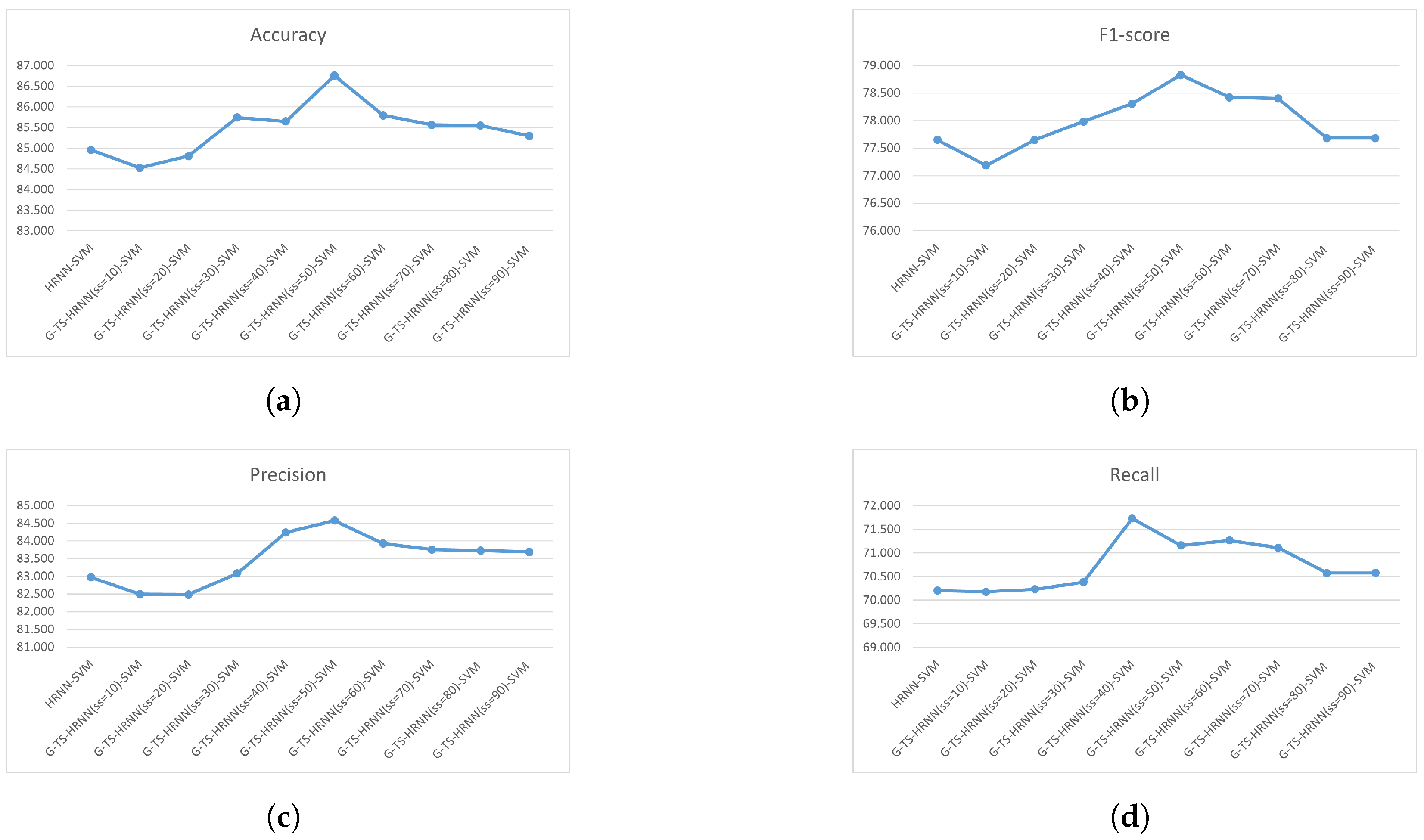
• Physics and Chemistry: the only data set from this field is wine. From Table 3, we have CI(G-TS-HRNN-SVM-50) = ±0.12; CI(G-TS-HRNN-SVM-60) = ±0.09; CI(G-TS-HRNN-SVM-70) = ±0.12. Thus, the most stable version in this field is G-TS-HRNN-SVM-60.
• Biology: the data sets from this field are Iris, Abalone, Ecoli, and Seed. From Table 3, we have CI(G-TS-HRNN-SVM-50) = ±0.20; CI(G-TS-HRNN-SVM-60) = ±0.17; CI(G-TS-HRNN-SVM-70) = ±0.14. Thus, the most stable version in this field is G-TS-HRNN-SVM-70.
• Health and Medicine: the data sets from this field are Liver, Spect, and Pima. From Table 3, we have CI(G-TS-HRNN-SVM-50) = ±0.18; CI(G-TS-HRNN-SVM-60) = ±0.17; CI(G-TS-HRNN-SVM-70) = ±0.13. Thus, the most stable version in this field is G-TS-HRNN-SVM-70.
• Social Science: the only data set from this field is Balance. From Table 3, we have CI(G-TS-HRNN-SVM-50) = ±0.19; CI(G-TS-HRNN-SVM-60) = ±0.16; CI(G-TS-HRNN-SVM-70) = ±0.12. Thus, the most stable version in this field is G-TS-HRNN-SVM-70.

We have computed the CPU time required by HRNN and TS-G-HRNN, considering several sizes (10 to 90), to teach SVM the classes of the UCI data sets given in Table 1; see

Table 4. CPU time required by HRNN and G-TS-HRNN to teach SVM the classes of UCI data sets.

	CPU time (s)
Data set/Method	HRNN-SVM	TS-HRNN-SVM(10)	TS-HRNN-SVM(20)	TS-HRNN-SVM(30)	TS-HRNN-SVM(40)
iris	1.71525	1.71234	1.71302	1.71363	1.72697
Wine	0.1676	0.16469	0.16537	0.16598	0.17932
Pima	2.8306	2.82769	2.82837	2.82898	2.84232
Haberman	0.0234	0.02049	0.02117	0.02178	0.03512
Balance	0.0086	0.00569	0.00637	0.00698	0.02032
Libra	0.0087	0.00579	0.00647	0.00708	0.02042
Liver	0.1294	0.12649	0.12717	0.12778	0.14112
Seed	0.0033	0.00039	0.00107	0.00168	0.01502
Spect	0.0054	0.00249	0.00317	0.00378	0.01712
Segment	0.0624	0.05949	0.06017	0.06078	0.07412
Vehicle	0.1581	0.15519	0.15587	0.15648	0.16982
	CPU time (s)
Data set/Method	TS-HRNN-SVM(50)	TS-HRNN-SVM(60)	TS-HRNN-SVM(70)	TS-HRNN-SVM(80)	TS-HRNN-SVM(90)
iris	1.74433	1.74855	1.76142	1.72725	1.75843
Wine	0.19668	0.20090	0.21377	0.17960	0.21078
Pima	2.85968	2.86390	2.87677	2.84260	2.87378
Haberman	0.05248	0.05670	0.06957	0.03540	0.06658
Balance	0.03768	0.04190	0.05477	0.02060	0.05178
Libra	0.03778	0.04200	0.05487	0.02070	0.05188
Liver	0.15848	0.16270	0.17557	0.14140	0.17258
Seed	0.03238	0.03660	0.04947	0.01530	0.04648
Spect	0.03448	0.03870	0.05157	0.01740	0.04858
Segment	0.09148	0.09570	0.10857	0.07440	0.10558
Vehicle	0.18718	0.19140	0.20427	0.16910	0.20128

. The convergence criterion considered in this context is the stability of neuron activation. To visualize the difference in computation time between the different methods, we calculated the average computation time required for all data sets; see Figure 8. We note that TS-G-HRNN-SVM versions with sample sizes below 30 require less computation time than HRNN-SVM. TS-G-HRNN-SVM versions with sample sizes between 40 and 60 require more computation time than HRNN-SVM but with a slight difference (0.01 s). This difference becomes more significant for instances with sample sizes above 70 (0.1 s). For all TS-G-HRNN-SVM instances with sample sizes below 90, the difference in computation time remains acceptable. Moreover, this difference almost explodes when the sample size exceeds 100. In fact, the time gap increased from 0.01 s to 0.1 s for the samples considered, showing the exponential evolution of cpu time as a function of sample size. This remains the major drawback of our method.

Finally, the proposed family of classification methods G-TS-HRNN-SVM performs better than HRNN-SVM in terms of accuracy, F1-Measure, precision, and recall. The most performant versions are G-TS-HRNN-SVM-50, G-TS-HRNN-SVM-60, and G-TS-HRNN-SVM-70. The most stable version, among all the considered fields (Biology, Social science, and Health and Medicine), is G-TS-HRNN-SVM-70 except in Physics and Chemistry, where G-TS-HRNN-SVM-60 is the most stable. The reason for the poor performance of low-sample versions of G-TS-HRNN-SVM is that the complexity of this model is not sufficient to reproduce the under-studied phenomena: this is the underlearning phenomenon. The cause of the poor performance of G-TS-HRNN-SVM versions with very high sample sizes is the high complexity of this model, which leads to rote learning of the phenomena studied: this is the overlearning phenomenon.

Furthermore, a better compromise between performance and computation time is to consider versions of G-TS-HRNN-SVM with sample sizes between 50 and 70. Moreover, given the exponential behavior of computation time as a function of sample size, 100 samples should not be exceeded.

6. Conclusions

Problem: Like all single-point metaheuristics, HRNN has certain drawbacks, such as being more likely to get stuck in local optima or miss global optima due to the use of a single point to explore the search space. Additionally, it is more sensitive to the initial point and operator, which can influence the quality and diversity of solutions. Furthermore, it can have difficulty with dynamic or noisy environments, as it can lose track of the optimal region or be misled by random fluctuations. Despite attempts, based on the choice of the Euler–Cauchy discretization step, these problems persist, and the initial activations still have a significant influence on the quality of the HRNN’s stability point.

Proposed solution: To overcome these shortcomings, this paper introduces a fuzzy HRNN population-based optimization method, namely Gaussian Takagi–Sugeno Hopfield Recurrent Neural Network (G-TS-HRNN-SVM). G-TS-HRNN-SVM associates a fuzzy variable with each neuron, with suitable fuzzy values described by Gaussian membership functions that cover the universe of discourse of the introduced fuzzy variables by adopting appropriate means and standard deviations. To build a sample of G-TS-HRNN-SVM, we randomly generate a Gaussian mean for each neuron. This leads to a Takagi–Sugeno rule with a linear differential equation as the premise. The fuzzy center of gravity is used to estimate the steady state of the initial nonlinear HRNN.

Tests and results: G-TS-HRNN-SVM is used to solve the random optimization method and solve the classification problem based on the support vector mathematical model. HRNN and G-TS-HRNN-SVM were tested on nine data sets found in UCI (Machine Learning Repository). The performance metrics considered in this work are accuracy, F1-measure, precision, and recall. Compared with the classical HRNN, G-TS-HRNN-SVM performs better on well-known data sets. First, the best G-TS-HRNN-SVM is the one with the mean number of rules (i.e., 40, 50, and 60). In addition, G-TS-HRNN-SVM permits an improvement of the classical HRNN accuracy (by 2.99%), F1-measure (by 4.16%), precision (by 3.83%), and recall (by 6.69%). Based on the confidence interval, the most stable version of G-TS-HRNN-SVM in the physics and chemistry fields is G-TS-HRNN-SVM(60), with CI = ±0.09; the most stable version in “biology”, with CI = ±0.14; and “health and medicine”, with CI = ±0.13, and “social science”, with CI = ±0.12, fields G-TS-HRNN-SVM(70).

Limitations: An instance of G-TS-HRNN-SVM with a very small sample size leads to underlearning and premature convergence, whereas an instance of G-TS-HRNN-SVM with a large sample size leads to overlearning and requires a very large memory size. In this context, selecting the best sample size remains a very difficult issue. In this respect, to avoid an explosion in calculation time, we must not exceed 100 samples, which is the main drawback of our method.

Future scope: In the future, we will use the genetic algorithm metaheuristic to realize the crossover and mutation operator between the rules within each sample to improve the quality of the solution. In addition, we will introduce the fractional version of G-TS-HRNN-SVM to handle more information about the problem to be solved. In addition, we will use G-TS-HRNN to perform the transformer and CNN learning tasks and perform self-association memory.

References

1. Mitra, S.; Hayashi, Y. Neuro-fuzzy rule generation: Survey in soft computing framework. IEEE Trans. Neural Netw. 2000, 11, 748–768. [Google Scholar] [CrossRef] [PubMed]
2. Shihabudheen, K.V.; Pillai, G.N. Recent advances in neuro-fuzzy system: A survey. Knowl.-Based Syst. 2018, 152, 136–162. [Google Scholar] [CrossRef]
3. Yen, J.; Wang, L.; Gillespie, C.W. Improving the interpretability of TSK fuzzy models by combining global learning and local learning. IEEE Trans. Fuzzy Syst. 1998, 6, 530–537. [Google Scholar] [CrossRef]
4. Du, M.; Behera, A.K.; Vaikuntanathan, S. Active oscillatory associative memory. J. Chem. Phys. 2024, 160, 055103. [Google Scholar] [CrossRef]
5. Abdulrahman, A.; Sayeh, M.; Fadhil, A. Enhancing the analog to digital converter using proteretic hopfield neural network. Neural Comput. Appl. 2024, 36, 5735–5745. [Google Scholar] [CrossRef]
6. Roudani, M.; El Moutaouakil, K.; Palade, V.; Baïzri, H.; Chellak, S.; Cheggour, M. Fuzzy Clustering SMOTE and Fuzzy Classifiers for Hidden Disease Predictions; Lecture Notes in Networks and Systems; Springer: Cham, Switzerland, 2024; Volume 1093. [Google Scholar]
7. El Moutaouakil, K.; Bouhanch, Z.; Ahourag, A.; Aberqi, A.; Karite, T. OPT-FRAC-CHN: Optimal Fractional Continuous Hopfield Network. Symmetry 2024, 16, 921. [Google Scholar] [CrossRef]
8. Uykan, Z. On the Working Principle of the Hopfield Neural Networks and its Equivalence to the GADIA in Optimization. IEEE Trans. Neural Netw. Learn. Syst. 2020, 31, 3294–3304. [Google Scholar] [CrossRef] [PubMed]
9. Talaván, P.M.; Yáñez, J. The generalized quadratic knapsack problem. A neuronal network approach. Neural Netw. 2006, 19, 416–428. [Google Scholar] [CrossRef] [PubMed]
10. Talaván, P.M.; Yáñez, J. A continuous Hopfield network equilibrium points algorithm. Comput. Oper. Res. 2005, 32, 2179–2196. [Google Scholar] [CrossRef]
11. El Ouissari, A.; El Moutaouakil, K. Intelligent optimal control of nonlinear diabetic population dynamics system using a genetic algorithm. Syst. Res. Inf. Technol. 2024, 1, 134–148. [Google Scholar]
12. Kurdyukov, V.; Kaziev, G.; Tattibekov, K. Clustering Methods for Network Data Analysis in Programming. Int. J. Commun. Netw. Inf. Secur. 2023, 15, 149–167. [Google Scholar]
13. Singh, H.; Sharma, J.R.; Kumar, S. A simple yet efficient two-step fifth-order weighted-Newton method for nonlinear models. Numer. Algorithms 2023, 93, 203–225. [Google Scholar] [CrossRef]
14. Bu, F.; Zhang, C.; Kim, E.H.; Yang, D.; Fu, Z.; Pedrycz, W. Fuzzy clustering-based neural network based on linear fitting residual-driven weighted fuzzy clustering and convolutional regularization strategy. Appl. Soft Comput. 2024, 154, 111403. [Google Scholar] [CrossRef]
15. Sharma, R.; Goel, T.; Tanveer, M.; Al-Dhaifallah, M. Alzheimer’s Disease Diagnosis Using Ensemble of Random Weighted Features and Fuzzy Least Square Twin Support Vector Machine. IEEE Trans. Emerg. Top. Comput. Intell. 2025; early access. [Google Scholar] [CrossRef]
16. Smith, K.A. Neural networks for combinatorial optimization: A review of more than a decade of research. Informs J. Comput. 1999, 11, 15–34. [Google Scholar] [CrossRef]
17. Joya, G.; Atencia, M.A.; Sandoval, F. Hopfield neural networks for optimization: Study of the different dynamics. Neurocomputing 2002, 43, 219–237. [Google Scholar] [CrossRef]
18. Wang, L. On the dynamics of discrete-time, continuous-state Hopfield neural networks. IEEE Trans. Circuits Syst. II Analog Digit. Signal Process. 1998, 45, 747–749. [Google Scholar]
19. Demidowitsch, B.P.; Maron, I.A.; Schuwalowa, E.S. Metodos Numericos de Analisis; Paraninfo: Madrid, Spain, 1980. [Google Scholar]
20. Bagherzadeh, N.; Kerola, T.; Leddy, B.; Brice, R. On parallel execution of the traveling salesman problem on a neural network model. In Proceedings of the IEEE International Conference on Neural Networks, San Diego, CA, USA, 21–24 June 1987; Volume III, pp. 317–324. [Google Scholar]
21. Brandt, R.D.; Wang, Y.; Laub, A.J.; Mitra, S.K. Alternative networks for solving the traveling salesman problem and the list-matching problem. In Proceedings of the International Conference on Neural Network (ICNN’88), San Diego, CA, USA, 24–27 July 1988; Volume II, pp. 333–340. [Google Scholar]
22. Wu, J.K. Neural Networks and Simulation Methods; Marcel Dekker: New York, NY, USA, 1994. [Google Scholar]
23. Abe, S. Global convergence and suppression of spurious states of the Hopfield neural networks. IEEE Trans. Circuits Syst. 1993, 40, 246–257. [Google Scholar] [CrossRef]
24. Wang, L.; Smith, K. On chaotic simulated annealing. IEEE Trans. Neural Netw. 1998, 9, 716–718. [Google Scholar] [CrossRef]
25. Jin, Q.; Mokhtari, A. Non-asymptotic superlinear convergence of standard quasi-Newton methods. Math. Program. 2023, 200, 425–473. [Google Scholar] [CrossRef]
26. Ogwo, G.N.; Alakoya, T.O.; Mewomo, O.T. Iterative algorithm with self-adaptive step size for approximating the common solution of variational inequality and fixed point problems. Optimization 2023, 72, 677–711. [Google Scholar] [CrossRef]
27. Gharbia, I.B.; Ferzly, J.; Vohralík, M.; Yousef, S. Semismooth and smoothing Newton methods for nonlinear systems with complementarity constraints: Adaptivity and inexact resolution. J. Comput. Appl. Math. 2023, 420, 114765. [Google Scholar] [CrossRef]
28. Candelario, G.; Cordero, A.; Torregrosa, J.R.; Vassileva, M.P. Generalized conformable fractional Newton-type method for solving nonlinear systems. Numer. Algorithms 2023, 93, 1171–1208. [Google Scholar] [CrossRef]
29. Dua, D.; Graff, C. UCI Machine Learning Repository; University of California, School of Information and Computer Science: Irvine, CA, USA, 2019; Available online: http://archive.ics.uci.edu/ml (accessed on 24 December 2024).
30. Breiding, P.; Rose, K.; Timme, S. Certifying zeros of polynomial systems using interval arithmetic. ACM Trans. Math. Softw. 2023, 49, 1–14. [Google Scholar] [CrossRef]
31. Bhuvaneswari, S.; Karthikeyan, S. A Comprehensive Research of Breast Cancer Detection Using Machine Learning, Clustering and Optimization Techniques. In Proceedings of the 2023 IEEE International Conference on Data Science and Network Security (ICDSNS), Tiptur, India, 28–29 July 2023. [Google Scholar]
32. Zimmermann, H.-J. Fuzzy Set Theory—And Its Applications, 4th ed.; Springer: Berlin/Heidelberg, Germany, 2010. [Google Scholar]
33. Rajafillah, C.; El Moutaouakil, K.; Patriciu, A.M.; Yahyaouy, A.; Riffi, J. INT-FUP: Intuitionistic Fuzzy Pooling. Mathematics 2024, 12, 1740. [Google Scholar] [CrossRef]
34. Sugeno, M.; Kang, G. Structure identification of fuzzy model. Fuzzy Sets Syst. 1988, 28, 15–33. [Google Scholar] [CrossRef]
35. Sugeno, M. Fuzzy Control; North-Holland, Publishing Co.: Amsterdam, The Netherlands, 1988. [Google Scholar]
36. Mehran, K. Takagi-sugeno fuzzy modeling for process control. Ind. Autom. Robot. Artif. Intell. 2008, 262, 1–31. [Google Scholar]
37. Kawamoto, S.; Tada, K.; Ishigame, A.; Taniguchi, T. An approach to stability analysis of second order fuzzy systems. In Proceedings of the IEEE International Conference on Fuzzy Systems, San Diego, CA, USA, 8–12 March 1992; pp. 1427–1434. [Google Scholar]
38. Tanaka, K. A Theory of Advanced Fuzzy Control; Springer: Berlin, Germany, 1994. [Google Scholar]
39. Mercer, J. Functions of positive and negative type, and their connection the theory of integral equations. Philos. Trans. R. Soc. Lond. 1909, 209, 415–446. [Google Scholar] [CrossRef]
40. Schölkopf, B.; Smola, A.J.; Bach, F. Learning with Kernels: Support Vector Machines, Regularization, Optimization, and Beyond; MIT Press: Cambridge, MA, USA, 2002. [Google Scholar]
41. Pandey, R.K.; Agrawal, O.P. Comparison of four numerical schemes for isoperimetric constraint fractional variational problems with A-operator. In Proceedings of the International Design Engineering Technical Conferences and Computers and Information in Engineering Conference, Boston, MA, USA, 2–5 August 2015; American Society of Mechanical Engineers: New York City, NY, USA, 2015; Volume 57199. [Google Scholar]
42. Kumar, K.; Pandey, R.K.; Sharma, S. Approximations of fractional integrals and Caputo derivatives with application in solving Abel’s integral equations. J. King Saud Univ.-Sci. 2019, 31, 692–700. [Google Scholar] [CrossRef]
Figure 1. Illustration of the sector nonlinearity approach.
Information 16 00141 g001
Figure 2. Membership functions for u 0 = 0.2 .
Information 16 00141 g002
Figure 3. Gaussian Takagi–Sugeno HRNN sampling, fuzzification, and equilibrium state approximation.
Information 16 00141 g003
Figure 4. Illustration of the approximation of the optimal steady state via the Takagi–Sugeno HRNN sampling method.
Information 16 00141 g004
Figure 5. The energy of the G-TS-HRNN for different sample sizes vs. the energy of the HRNN at a steady point.
Information 16 00141 g005
Figure 6. Takagi–Sugeno HRNN robustness.
Information 16 00141 g006
Figure 7. Mean accuracy (a), mean F1-score (b), mean precision (c), and mean recall (d), on all data sets of the HRNN-SVM and the nine samples of G-TS-HRNN-SVM.
Information 16 00141 g007
Figure 8. Mean cpu time required by HRNN and G-TS-HRNN.
Information 16 00141 g008