On Exploiting Rating Prediction Accuracy Features in Dense Collaborative Filtering Datasets

Dimitris Spiliotopoulos; Dionisis Margaris; Costas Vassilakis

doi:10.3390/info13090428

,

and

¹

Department of Management Science and Technology, University of the Peloponnese, Akadimaikou G. K. Vlachou, 22131 Tripoli, Greece

²

Department of Digital Systems, University of the Peloponnese, Valioti’s Building, Kladas, 23100 Sparta, Greece

³

Department of Informatics and Telecommunications, University of the Peloponnese, Akadimaikou G. K. Vlachou, 22131 Tripoli, Greece

^*

Author to whom correspondence should be addressed.

Information2022, 13(9), 428;https://doi.org/10.3390/info13090428

This article belongs to the Special Issue Recommendation Algorithms and Web Mining

Version Notes

Order Reprints

Abstract

One of the typical goals of collaborative filtering algorithms is to produce rating predictions with values very close to what real users would give to an item. Afterward, the items having the largest rating prediction values will be recommended to the users by the recommender system. Collaborative filtering algorithms can be applied to both sparse and dense datasets, and each of these dataset categories involves different kinds of risks. As far as the dense collaborative filtering datasets are concerned, where the rating prediction coverage is, most of the time, very high, we usually face large rating prediction times, issues concerning the selection of a user’s near neighbours, etc. Although collaborative filtering algorithms usually achieve better results when applied to dense datasets, there is still room for improvement, since in many cases, the rating prediction error is relatively high, which leads to unsuccessful recommendations and hence to recommender system unreliability. In this work, we explore rating prediction accuracy features, although in a broader context, in dense collaborative filtering datasets. We conduct an extensive evaluation, using dense datasets, widely used in collaborative filtering research, in order to find the associations between these features and the rating prediction accuracy.

Keywords:

collaborative filtering; recommender systems; personalisation; dataset density; rating prediction accuracy; accuracy features; evaluation

1. Introduction

One of the most widely applied recommender system (RS) methods, over the last 20 years, is collaborative filtering (CF) [1,2]. The typical goal of a CF algorithm is to produce rating predictions for products or services that users have not already evaluated. The closer these rating predictions are to the rating values that the users themselves would give to these products or services, the higher accuracy the CF algorithm will have.

Afterwards, based on the aforementioned rating predictions, a CF RS will typically recommend, to each user, the products or services scoring higher rating prediction values. These products carry the highest probability, among all products or services, that the user will actually like them and hence accept the recommendation (by clicking the product advertisement, buying the product or service, etc.) [3,4].

The first step of a typical CF system is to locate the ‘near neighbours’ (NNs) for each of its users. An NN of user u is another user v who shares similar likings with u. This can be found by taking the stored real ratings of users u and v, set_of_ratings_u, and set_of_ratings_v, finding the ones given to common products or services i (i.e., the intersection of the two sets), and comparing them. If the majority of them are (to a large extent) similar, then these users are NNs with each other [5,6]. Typically, in modern CF RSs, the aforementioned task is implemented using a user vicinity metric, such as the Pearson correlation coefficient (PCC) and the cosine similarity (CS), which quantify the vicinity between two CF users with a numeric value [7,8].

The second step of a typical CF system is to compute a rating prediction value rpv_u,i of user u to the product i; for this process, the CF system uses the real ratings of u’s NNs (found in the previous step) to the same item. The rationale behind this setting is that, in the real world, a person usually trusts the people considered closer to him/her (higher vicinity), when asking for a recommendation, regardless of the product or service category [9,10].

The accuracy of CF systems is measured by the closeness of the rating prediction values to the real user rating values. Accuracy is a very active research field, where the majority of the research works aim at reducing the overall deviation between the predicted values of the ratings that the users would give to the products and the values of real user ratings to the products. In order to evaluate the success of the aforementioned process, the CF algorithms are applied to real CF rating datasets (such as the Amazon and the MovieLens datasets [11,12]), usually containing records consisting of the user, the product, the rating, and maybe additional information (from the rating timestamp to information concerning the user and/or the product). Accuracy is evaluated by hiding a percentage of the ratings, then trying to predict their values, and finally assessing how close the prediction is to the real rating.

Despite a plethora of research works aiming to increase the CF rating prediction accuracy [13,14,15], very limited research aims to examine the characteristics of CF users, products, or the dataset itself, which may affect the accuracy of CF rating predictions. An exception is the work of researchers that utilise the user neighbourhood [16,17,18,19]. These works have been performed, in general, for evaluating the performance of specific algorithms.

Our previous work [20] explored the accuracy of rating prediction features in sparse CF datasets, in a broader context, proving that a typical CF system which simply recommends the items achieving higher rating prediction values than others may offer reduced recommendation accuracy, in many cases, and hence negatively affect the success of the RS.

In this paper, we adapt the aforementioned research in the context of dense CF datasets. More specifically:

We explore the same rating prediction accuracy features in dense CF datasets but with different parameter values. For example, our previous work showed that, for sparse CF datasets, when a rating prediction is formulated using the real ratings of ≥4 NNs, it is an indication of a highly accurate rating prediction. For dense CF datasets, however, a user can have hundreds or even thousands of NNs. As a result, the percentage of the rating predictions formulated with ≥4 NNs is almost 100% and hence the output of the previous work cannot be applied in dense CF datasets;
We examine (evaluate and parameterise) the effects of one extra rating prediction accuracy feature, namely the NN variety, which, in contrast to sparse CF datasets, can be reliably quantified in dense CF datasets.

To ascertain the reliability of the results produced, the present work uses (i) two widely accepted metrics of user similarity, (ii) two widely accepted rating prediction error metrics, (iii) six widely accepted dense CF datasets, and (iv) three different CF algorithms, so that it can experimentally derive insight on the rating prediction accuracy features.

The rest of the paper is structured as follows: Section 2 overviews the related work, while in Section 3, we present, analyse, and evaluate the rating prediction features in dense CF datasets. The obtained results are discussed in Section 4, and Section 5 concludes the paper and outlines future work. The definitions for terms, notations, and abbreviations used in this paper are tabulated in Table 1.

Table 1. Definitions for terms, notations, and abbreviations used.

2. Related Work

The CF system accuracy research is divided into two main categories. The first category comprises algorithms which, apart from the basic information a CF system needs in order to produce rating predictions (i.e., the user–item–rating matrix), utilise supplementary elements or sources of information. These include user and item information, such as user relations in social networks (SNs) (friendship, trust, etc.), user demographic information (gender, age, nationality, etc.), item categories (e.g., taxonomy) and characteristics (colour, price, availability, etc.), user reviews on an item, etc. The second category comprises algorithms that exploit only the basic CF information and the user–item–rating matrix and formulate specialised processing methods (e.g., the clustering, computation, and exploitation of outliers, rating variability, etc.) to increase the rating prediction accuracy.

Regarding the first category, Yang et al. [21] introduced a matrix factorisation (MF) technique which improves the performance of CF recommendations by integrating the sparse social trust network data with the sparse user rating data, among the same users. Their model-based technique maps CF users, based on their trust relationship, into low-dimensional latent feature spaces, and aims to reflect the users’ reciprocal influence on the formation of their own ratings. Yang et al. [22] presented a set of MF- and NN-based RS and explore group affiliations and SN information for recommendations in social voting. They demonstrated that the aforementioned information can improve the accuracy of popularity-based voting recommendations. They also observed that group and social information was proven to be more valuable to cold users. Hu et al. [23] presented a technique, namely MR3, which aligns the latent factors and hidden topics, in order to model item reviews and social relations with ratings, for improving the rating prediction accuracy. Furthermore, they incorporated the implicit feedback from ratings into their model, to enhance their technique. Margaris et al. [18] introduced an algorithm which combines the limited SN information of users’ social relations with the limited CF information of users’ ratings on items targeting the enhancement of both the rating prediction coverage and rating prediction accuracy in CF RSs. Their algorithm takes into account the utility and density of both CF and SN neighbourhoods, by formulating two partial rating predictions: the CF score and the SN score. Then, it combines these scores using a weighted average metascore algorithm with user-personalised weights. Pereira and Varma [24] presented a financial planning RS that modifies the recommendation process to enhance the recommendations. They used a hybrid approach to overcome CF drawbacks, such as data sparsity, the new user cold-start problem, and overspecialisation, which combines CF techniques with demographic filtering. Ghasemi and Momtazi [25] introduced a technique that improves CF RSs by finding similar CF users based on both their ratings and reviews. They utilised two lexical-based techniques, two word-neural representation techniques, and three text-neural representation techniques. Zhou et al. [26] introduced MLCF, a multi-label classification-based CF framework that enhances the recommendation quality, which is based on three graphs, namely a user, an item, and a rating bipartite. They explored the latent correlations among items and users. They also introduced a multi-label classification rating similarity metric which captures user-class-specific relationships. Finally, they introduced the integration of two multi-label classification CF techniques, focusing on social information and rating, into a unified rating prediction technique.

Although all the aforementioned works considerably enhance the CF rating prediction accuracy and recommendation success, the source of supplementary information that is required (user SN information, user demographic information, user and item characteristics, etc.) may not always be available and, hence, cannot be applied to every CF dataset.

To this extent, Wang et al. [27] proposed the integration of the interactions between items and users. They introduced the neural graph CF, a recommendation framework that propagates embeddings on the user–item graph structure, which explicitly injects, into the embedding process, the collaborative signal. Yu et al. [28] proposed a two-sided cross-domain CF model, which balances recommendation efficiency and accuracy. This model is based on selective ensemble learning considering both efficiency and accuracy. Their model first combines the item-sided with the user-sided auxiliary domains, aiming to enhance the target domain performance. The cross-domain CF problem is then transformed into an ensemble learning problem, thereby transforming the selective combination problem into a selective classifier problem. Ajaegbu [29] introduced an algorithm which balances three user similarity metrics to overcome cold-start issues. This algorithm mitigates the data sparsity and cold-start issues that the three traditional algorithms face, as well as retains the positive features the existing item-based CF algorithms have. Margaris et al. [30] presented an algorithm which improves the rating prediction accuracy in CF without the need for any kind of supplementary information. They achieved accuracy improvement by enhancing the weight of the black sheep NNs’ opinions. More specifically, they adjusted the NN weights, based on the degree to which the NN and the target user deviate from each of the dominant ratings of each item. Zarzour et al. [31] introduced a new CF algorithm based on clustering techniques and dimensionality reduction. The proposed algorithm uses singular value decomposition to reduce the dimensionality, while it uses the K-means algorithm in order to cluster similar users. They also proposed and assessed a two-stage RS which produces efficient and accurate recommendations. Neysiani et al. [32] presented a method that produces association rules, based on genetic algorithms, which identify these association rules in an unsupervised manner, while at the same time, they are efficient for space search. For this method, the users do not need to specify support thresholds. Additionally, in contrast to traditional mining models, it does not need to discover a large number of rules. Chen et al. [33] presented a CF recommendation technique based on evolutionary clustering and user correlation. The authors pre-processed the rating matrix with dimension reduction and normalisation to obtain denser rating data. They used dynamic evolutionary clustering and the highest similar-interest NN research. Finally, they proposed a user relationship metric that applies potential information and user satisfaction.

Still, none of the aforementioned research works examines those features related to the rating prediction accuracy in CF datasets. An RS that typically recommends the items computed to have the highest rating prediction scores, without taking into account other features, may result in reduced recommendation accuracy and overall success and, hence, cause trust issues in its users.

Recently, Margaris et al. [20] indicated that it may be better for an RS to recommend an item i2 computed to have a lower prediction value than item i1, if the rating prediction concerning i2 is found to be more reliable than the respective one for i1, by exploring, in a broader context, the rating prediction accuracy features in sparse CF datasets. They examined five rating prediction features, using sparse CF datasets, and found that three of them (the number of NNs participating in the rating prediction formulation, the mean rating value of the active user, and the mean rating value of the item) can indicate, in the majority of the cases, a reliable rating prediction.

The present work advances the state-of-the-art research regarding the rating prediction accuracy features in CF, by (1) applying and parameterising the aforementioned rating prediction accuracy features in dense CF datasets, (2) applying and parameterising an additional rating prediction accuracy feature that can be reliably applied only in dense CF datasets, and (3) evaluating the rating prediction accuracy features using widely used and accepted dense CF datasets, error metrics, and user similarity metrics. Since the features tested in this work are derived from the original rating matrix (user–item–rating tuple) and do not need any kind of additional information, they prove useful to any CF algorithm applied to dense CF datasets.

3. Exploring Rating Prediction Features

In this section, the six rating prediction features of the experimental part of our work are presented, analysed, and evaluated. More specifically, we present a thorough investigation of the rating prediction features, examining their associations with improvement in the rating prediction accuracy in dense CF datasets.

The six rating prediction features, along with their cases tested in the experimental procedure, are the following:

The percentage of the active user U’s near neighbours (NNs) taking part in the rating prediction (NN%): for this feature, we examined values from 0% to 24%, with the increment step set to 3%;
The active user’s U average rating value (U_avg): for this feature, we examined the range from the minimum allowed rating value to the maximum allowed rating value in the dataset, with the increment step set to 0.5;
The average rating value of the item for which the prediction is computed (I_avg): for this feature, we examined the range from the minimum allowed rating value to the maximum allowed rating value in the dataset, with the increment step set to 0.5;
The number of items that the active user U has rated (U_N): for this feature, we examined values from 100 to 500, and an extra case of >500, with the increment step set to 100;
The number of users that have rated item i for which the prediction is computed (I_N): for this feature, we examined values from 100 to 500 and an extra case of >500, with the increment step set to 100;
The variance of the NNs’ ratings given to the item for which the prediction is computed (NNs_var): for this feature, we examined values from 0.0 to 2.5, and an extra case of >2.5 with the increment step set to 0.25.

To ascertain that our work is NN-independent, measurements were obtained using all the NNs each active user has, setting the NN vicinity threshold to 0.0 [20,34,35].

In our experiments, we used CF datasets that are widely accepted and used in CF research [36,37,38]. All datasets are relatively dense (their densities range from 0.13% to 5.88%); Table 2 presents their essential information [12,39,40,41]. While there is no agreed threshold for classifying a dataset as “dense” or “sparse”, the density of all the datasets examined in this work is at least 60% higher than the density of the datasets examined in our previous work [20], which are characterised as “sparse”. The density of a dataset d is defined as the ratio of the number of elements of the user–item rating matrix that have non-null values to the total number of the elements of the user–item rating matrix. Density can be computed as

d = \frac{# R a t i n g s}{# U s e r s * # I t e m s}

. To ascertain that a single rating value range was used, in order for the results of the different datasets to be comparable, the ratings in each dataset were normalised in the range [1.0–5.0], using the standard min–max formula [42], which is used in many CF research works [43,44,45].

Table 2. Dataset information.

In order to quantify the rating prediction accuracy, the following two CF rating prediction error metrics were used [46,47]:

The mean average error (MAE) metric, which handles all errors uniformly;
The root-mean-squared error (RMSE) metric, which boosts the significance of large deviations between the real user rating and the rating prediction produced by the CF system.

To compute the deviation between the rating prediction and the real rating value, the typical “hide-one” technique [48,49] was used for all the ratings in each dataset (where we sought to predict the value of all the ratings—one at a time—in the dataset). In more detail, each time one rating of the dataset is hidden, its value is predicted using the non-hidden ratings. “The “hide-one” or “leave-one-out cross-validation” approach is widely used in CF works [50,51,52], and it has the advantage of producing model estimates with less bias and more ease [53]. Its main disadvantage is that it cannot be applied online in very large datasets (due to the number of computational steps); however, in our work, it was performed offline.

To ascertain that our work is algorithm-independent, we obtained measurements using three different CF algorithms:

A “plain” CF algorithm [54,55];
A sequential CF algorithm [56];
A CF algorithm which exploits common rating histories until the review time of the item for which the prediction is being formulated [57].

A close agreement between the results from all the experiments was observed (less than 4% difference in all the cases); hence, for conciseness, we report only the results produced by the plain CF algorithm.

3.1. The NNs’ Percentage Taking Part in the Rating Prediction

Figure 1 illustrates the MAE observed for the six aforementioned dense datasets, considering the NN% feature and using the PCC user similarity metric.

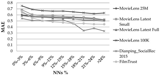
Figure 1. Effect of the NN% feature, in the rating prediction MAE, when the PCC user similarity metric was used.

For all the datasets, when the percentage of the NNs taking part in the rating prediction increased, an MAE drop was observed, until this percentage reached the value of 15%. After that value, a different behaviour between the datasets was observed; the MAE change became non-monotonic. However, for all the cases, the MAE for values of NN% exceeding 15% was less than the MAE at NN% = 15%. The average MAE and RMSE reductions from the case of NN% ≈ 0% to the case of NN% = 15% were measured to be equal to 13% and 12%, respectively. When the CS user similarity metric was used, the exact same phenomenon was observed. More specifically, the average MAE and RMSE reductions from the case of NN% ≈ 0% to the case of NN% = 15% were measured to be equal to 10% and 9%, respectively.

Overall, we can conclude that a correlation exists between the NN% feature and the rating prediction accuracy in dense CF datasets.

3.2. U_avg Feature

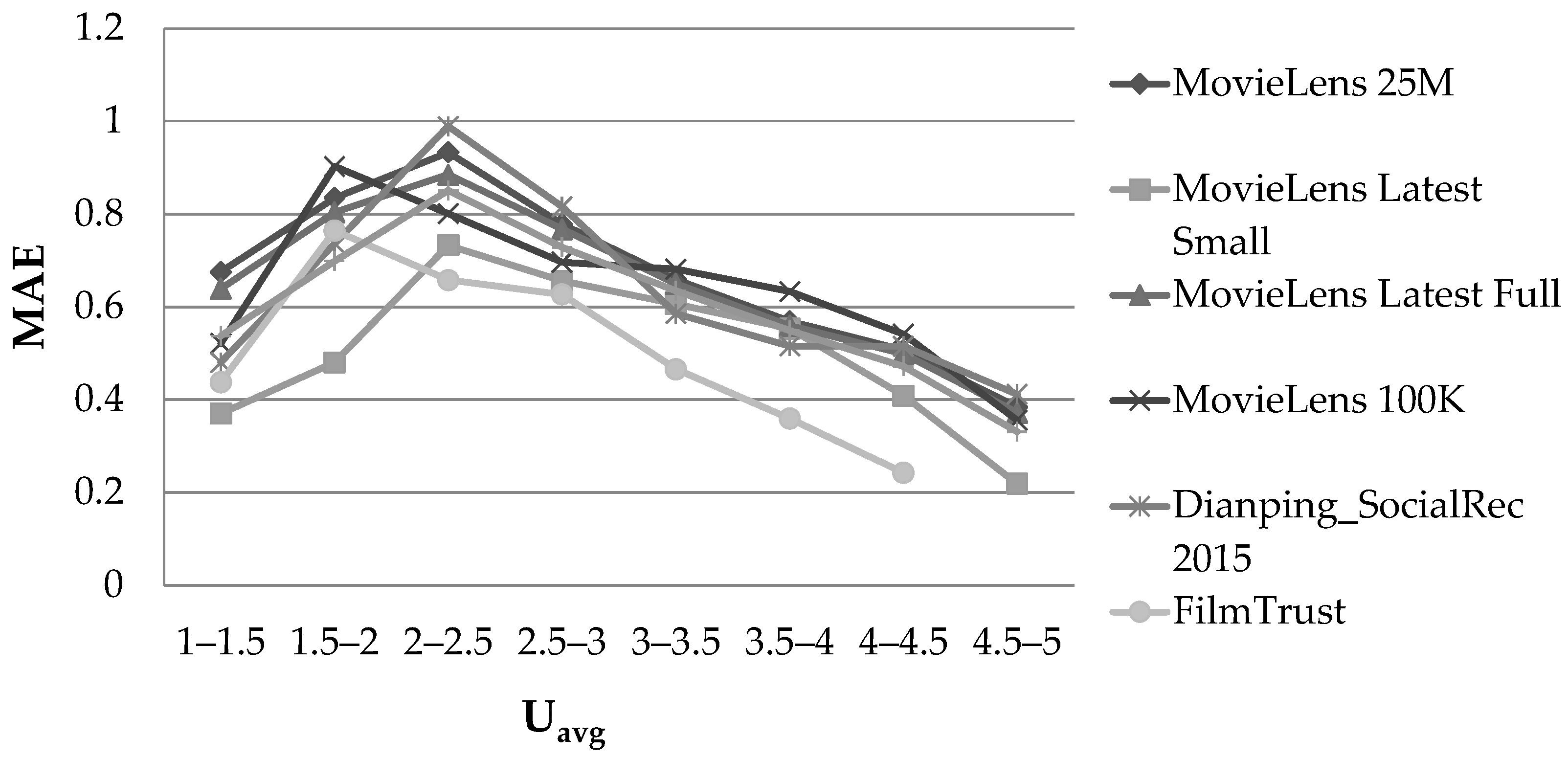
Figure 2 illustrates the MAE observed on the datasets, considering the U_avg feature and using the PCC user similarity metric.

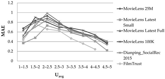
Figure 2. Effect of the U_avg feature, in the rating prediction MAE, when the PCC user similarity metric was used.

When the active user’s mean rating value was in the middle of the rating range (2 ≤ U_avg ≤ 3), the prediction accuracy was low, a fact that is reflected in the value of the MAE. This is in contrast to the case when the active user’s mean rating value was close to the rating range’s boundaries, and especially to the higher one (U_avg ≥ 4.5). In the latter case, the average MAE and RMSE observed were lower by 61% and 50%, respectively, when compared with the case in which the active user’s mean rating value was in the middle of the rating range (2 ≤ U_avg ≤ 3). When the CS user similarity metric was used, the exact same phenomenon was observed. More specifically, the average MAE and RMSE observed for the cases in which the user’s mean rating was close to the upper rating scale boundary were 53% and 46% smaller, respectively, when compared with the case in which the active user’s mean rating value was in the middle of the rating range (2 ≤ U_avg ≤ 3). Notably, this behaviour pattern was observed in all the datasets, regardless of their density, since the dataset density had no impact on the U_avg quantity.

Overall, we can again conclude that a correlation exists between the U_avg feature and the rating prediction accuracy in dense CF datasets.

3.3. I_avg Feature

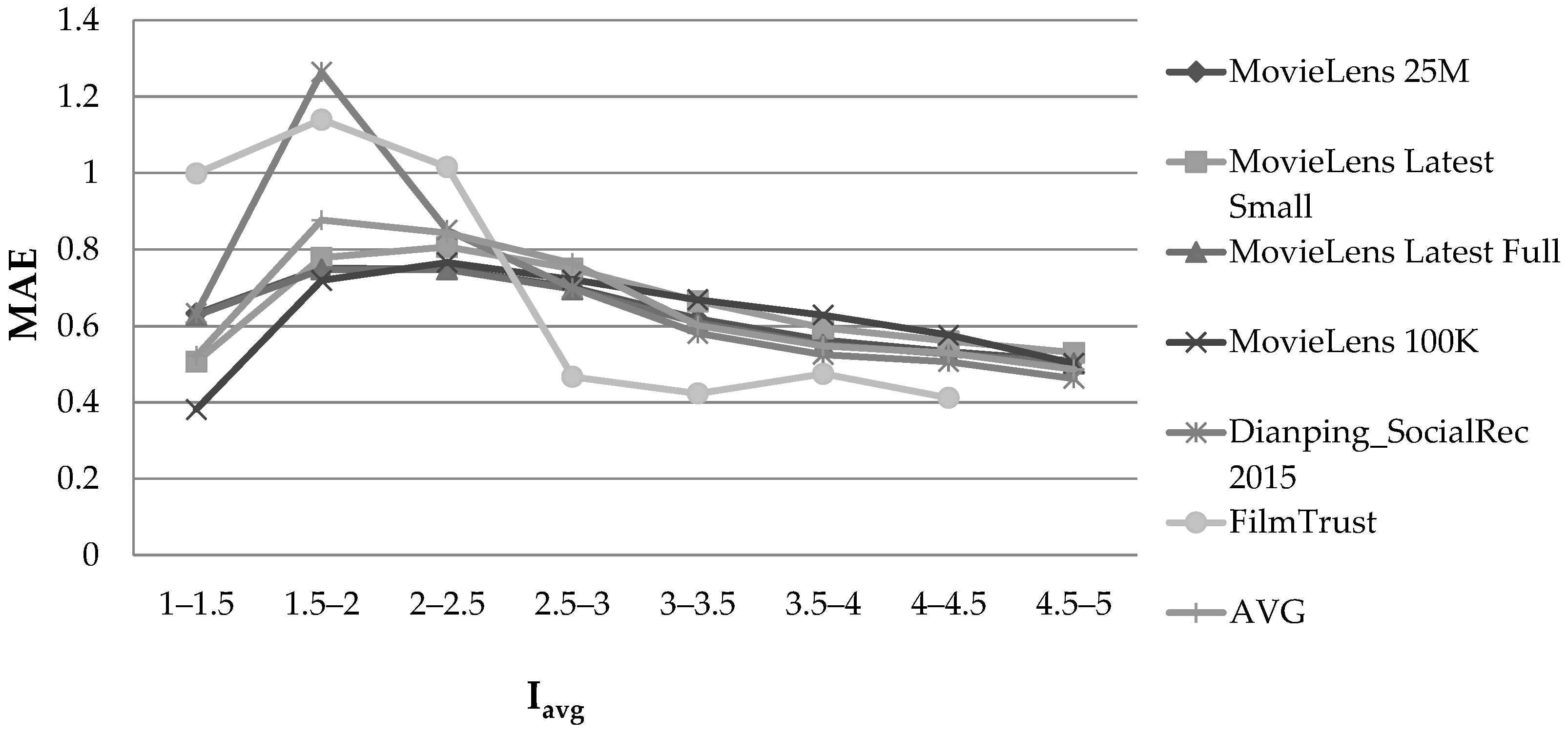
Figure 3 illustrates the MAE observed on the datasets, considering the I_avg feature and using the PCC user similarity metric.

Figure 3. Effect of the I_avg feature, in the rating prediction MAE, when the PCC user similarity metric was used.

When the active item’s mean rating value was towards the low end of the rating range but not very close to it (1.5 ≤ I_avg ≤ 2.5), the prediction accuracy was low. Conversely, when the mean rating value of the active item is close to the boundaries of the rating range, the prediction accuracy is high, especially in the higher rating range. This was especially evident for values close to the upper boundary (I_avg ≥4.5). In the latter case, the average MAE and RMSE observed were 42% and 37% smaller, respectively, when compared with those of the case in which the active item’s mean rating value was in the “low-accuracy” area (1.5 ≤ I_avg ≤ 2.5). When the CS user similarity metric was used, the exact same phenomenon was observed. More specifically, the average MAE and RMSE observed were 40% and 37% reduced, respectively, when compared with those of the case in which the mean rating value of the active item was in the “low-accuracy” area (1.5 ≤ I_avg ≤ 2.5).

Overall, we can again conclude that a correlation exists between the I_avg feature and the rating prediction accuracy in dense CF datasets.

3.4. U_N Feature

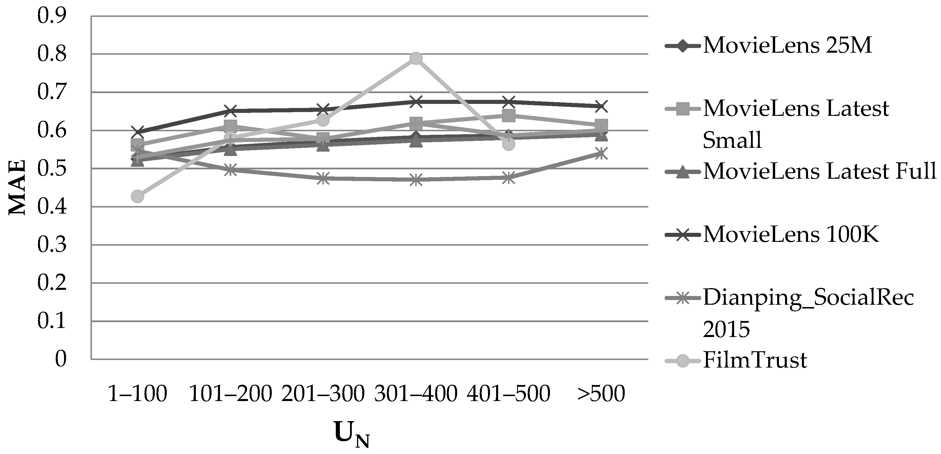
Figure 4 illustrates the MAE observed on the datasets, considering the U_N feature and using the PCC user similarity metric.

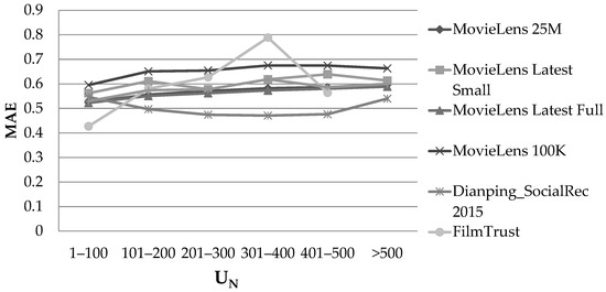
Figure 4. Effect of the U_N feature, in the rating prediction MAE, when the PCC user similarity metric was used.

A divergent behaviour was observed among the six datasets when the U_N feature’s value increased, while, in general, no clear minima or maxima could be identified when the value of U_N varied. Hence, no correlation can be established between the U_N feature and the rating prediction accuracy in dense CF datasets.

3.5. I_N Feature

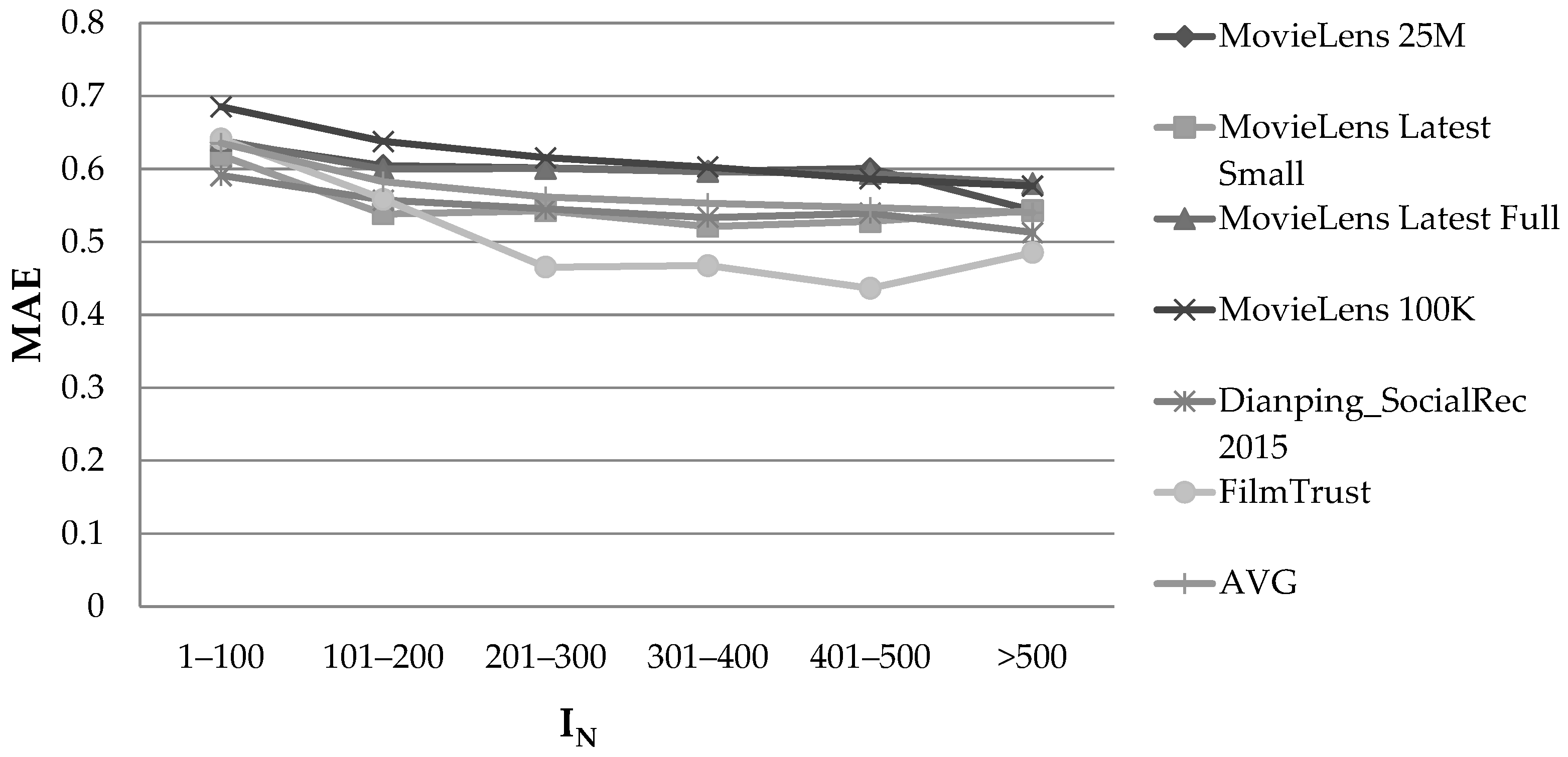
Figure 5 illustrates the MAE observed on the datasets, considering the I_N feature and using the PCC user similarity metric.

Figure 5. Effect of the I_N feature, in the rating prediction MAE, when the PCC user similarity metric was used.

A divergent behaviour was again observed among the six datasets when the value of the I_N feature increased, and, in general, no clear minima or maxima could be identified when the value of U_N varied. Hence, no correlation can be established between the I_N feature and the rating prediction accuracy in dense CF datasets.

3.6. NNs_var Feature

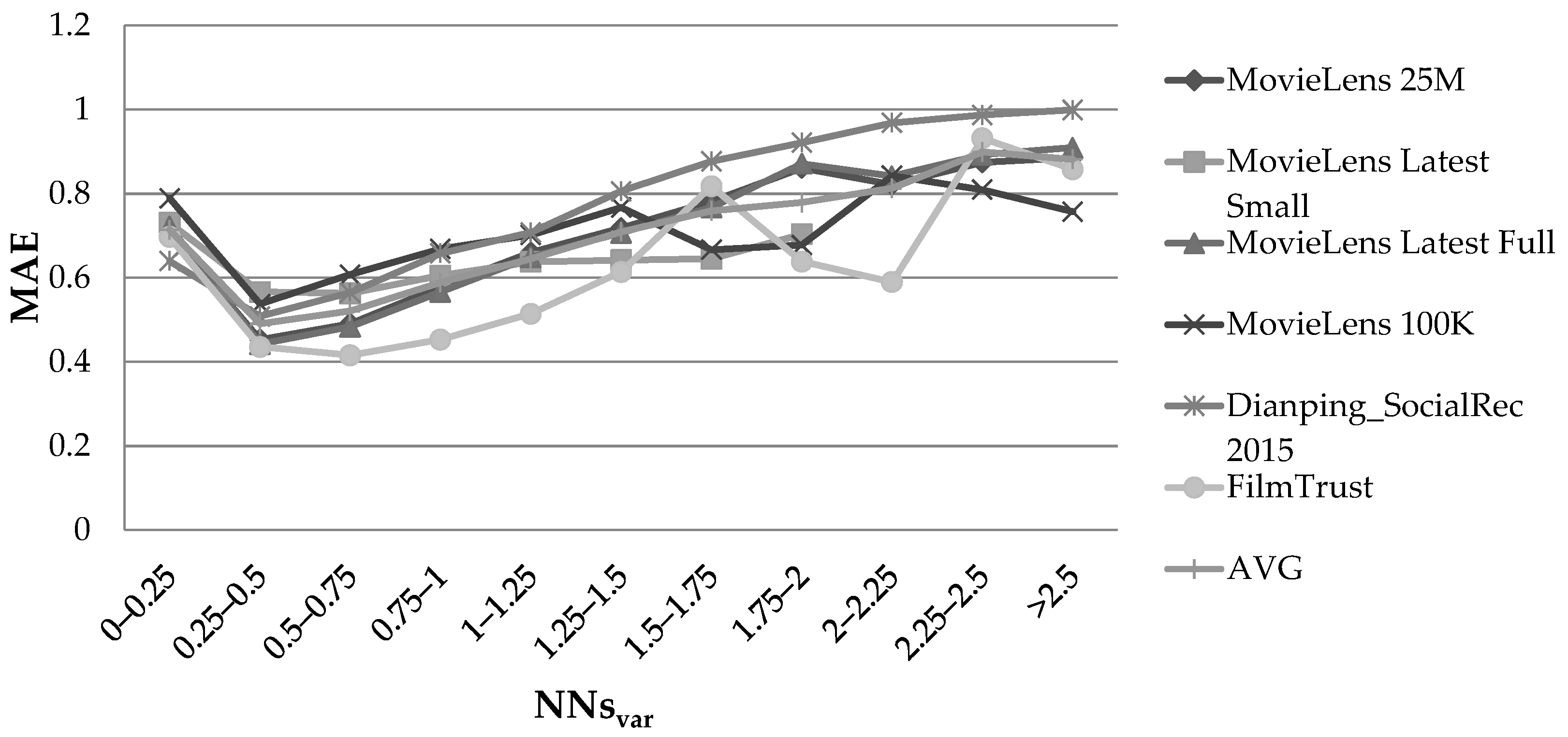
Figure 6 illustrates the MAE observed on the datasets, considering the NNs_var feature and using the PCC user similarity metric.

Figure 6. Effect of the NNs_var feature, in the rating prediction MAE, when the PCC user similarity metric was used.

When the variance of the NNs’ ratings to the item for which the prediction was being formulated was relatively low, especially in the range of 0.25–0.75, a high level of prediction accuracy was observed. More specifically, the average MAE reduction from the cases when I_VAR > 2.5 to 0.25 ≤ I_VAR ≤ 0.75 equalled 43%, while the respective average RMSE reduction equalled 40%. When the CS user similarity metric was used, we observed the exact same phenomenon. More specifically, the average MAE and RMSE reductions from I_VAR > 2.5 to 0.25 ≤ I_VAR ≤ 0.75 were measured to be equal to 33% and 27%, respectively.

Overall, we can conclude that a correlation exists between the NN% feature and the rating prediction accuracy in dense CF datasets.

4. Discussion of the Results

From the experimental evaluation presented in the previous section, we can conclude that, in dense CF datasets, a CF rating prediction was found to be more reliable in the following cases:

The percentage of the active user’s NNs taking part in the rating prediction was ≥15%: when taking into account ≥ 15% of a user’s NNs, the CF rating prediction was considered more sound, due to the fact that, as in real life, a recommendation based on many opinions bears a high success probability;
The active user’s mean rating value was close to the limits of the rating range: it is much easier for a rating prediction system to predict the next rating of a user who almost always enters either excellent or bad ratings.
The predicted item’s mean rating value was close to the limits of the rating range: it is much easier for a rating prediction system to predict the next rating for an item that is practically considered either widely acceptable or unacceptable.
The variance of the user’s NNs’ ratings to the predicted item was relatively low (in the 0.25–0.75 range): it is easier for a rating prediction system to predict a rating for a user whose close people share similar opinions (either good or bad) for an item.

Using the above findings, the accuracy of an RS can be significantly improved, since the RS may opt not to recommend an item with a high prediction score that is, however, deemed of low reliability but include an alternative item in the recommendation which may have a slightly lower prediction but is associated with high confidence.

It is worth noting that the FilmTrust dataset exhibited different behaviour than the other datasets used in the experiments, in particular regarding the I_avg and U_N features (Figure 3 and Figure 4). The diverging behaviour observed in Figure 3 is due to the predictions related to those items with low I_avg values, the variance of which was found to be very high in this dataset. Notably, the FilmTrust dataset had the lowest rating average among all the datasets (3.00 against 3.53 of the MovieLens datasets and 3.74 in the Dianping SocialRec 2015 datasets). The deviating behaviour in Figure 4 is attributed to the fact that, in the FilmTrust dataset, most users have rated few items, and consequently, the FilmTrust data points were associated with high U_N data values (ranges of 301–400 and 401–500) practically representing outliers (less than 20 users per range), while the data point corresponding to the range “>500” was missing because no user had more than 500 ratings in this dataset. A more in-depth analysis of the effect of the statistical distribution of dataset features and skews on the behaviour of the dataset will be considered in our future work.

5. Conclusions and Future Work

In this work, six rating prediction accuracy features in dense CF datasets, with the aim to determine whether they directly affect the rating prediction accuracy, were explored. To ascertain the reliability of the results produced, two widely accepted metrics of user similarity, two widely accepted rating prediction error metrics, six widely accepted dense CF datasets, and three different CF algorithms were used to experimentally provide insight into the rating prediction accuracy features.

The evaluation results showed that (a) the percentage of the active user’s NNs taking part in the rating prediction, (b) the active user’s mean rating value, (c) the predicted item’s mean rating value, and (d) the variance of the active user NNs’ ratings in relation to the predicted item were correlated with the reduction in the rating prediction accuracy.

In our future work, we plan to refine the CF rating prediction algorithm, by quantifying the reliability of a CF rating prediction, based on the four prediction features that were found to affect the rating prediction accuracy in this work. Moreover, we will focus on exploring additional rating prediction features in dense CF datasets.

Author Contributions

Conceptualisation, D.S., D.M. and C.V.; methodology, D.S., D.M. and C.V.; software, D.S., D.M. and C.V.; validation, D.S., D.M. and C.V.; formal analysis, D.S., D.M. and C.V.; investigation, D.S., D.M. and C.V.; resources, D.S., D.M. and C.V.; data curation, D.S., D.M. and C.V.; writing—original draft preparation, D.S., D.M. and C.V.; writing—review and editing, D.S., D.M. and C.V.; visualisation, D.S., D.M. and C.V.; supervision, D.S., D.M. and C.V.; project administration, D.S., D.M. and C.V. All authors have read and agreed to the published version of the manuscript.

Funding

This research received no external funding.

Institutional Review Board Statement

Not applicable.

Informed Consent Statement

Not applicable.

Data Availability Statement

Publicly available datasets were analysed in this study. These data can be found here: https://grouplens.org/datasets/movielens/; https://guoguibing.github.io/librec/datasets.html; and https://lihui.info/data/dianping/ (accessed on 20 July 2022).

Conflicts of Interest

The authors declare no conflict of interest.

References

Lara-Cabrera, R.; González-Prieto, Á.; Ortega, F. Deep Matrix Factorization Approach for Collaborative Filtering Recommender Systems. Appl. Sci. 2020, 10, 4926. [Google Scholar] [CrossRef]
Cui, Z.; Xu, X.; Xue, F.; Cai, X.; Cao, Y.; Zhang, W.; Chen, J. Personalized Recommendation System Based on Collaborative Filtering for IoT Scenarios. IEEE Trans. Serv. Comput. 2020, 13, 685–695. [Google Scholar] [CrossRef]
Balabanović, M.; Shoham, Y. Fab: Content-Based, Collaborative Recommendation. Commun. ACM 1997, 40, 66–72. [Google Scholar] [CrossRef]
Cechinel, C.; Sicilia, M.-Á.; Sánchez-Alonso, S.; García-Barriocanal, E. Evaluating Collaborative Filtering Recommendations inside Large Learning Object Repositories. Inf. Process. Manag. 2013, 49, 34–50. [Google Scholar] [CrossRef]
Herlocker, J.L.; Konstan, J.A.; Terveen, L.G.; Riedl, J.T. Evaluating Collaborative Filtering Recommender Systems. ACM Trans. Inf. Syst. 2004, 22, 5–53. [Google Scholar] [CrossRef]
Park, Y.; Park, S.; Jung, W.; Lee, S. Reversed CF: A Fast Collaborative Filtering Algorithm Using a k-Nearest Neighbor Graph. Expert Syst. Appl. 2015, 42, 4022–4028. [Google Scholar] [CrossRef]
Sinha, B.B.; Dhanalakshmi, R. A Recommender System Based on a New Similarity Metric and Upgraded Crow Search Algorithm. IFS 2020, 39, 3167–3182. [Google Scholar] [CrossRef]
Mazurowski, M.A. Estimating Confidence of Individual Rating Predictions in Collaborative Filtering Recommender Systems. Expert Syst. Appl. 2013, 40, 3847–3857. [Google Scholar] [CrossRef]
Ning, H.; Dhelim, S.; Aung, N. PersoNet: Friend Recommendation System Based on Big-Five Personality Traits and Hybrid Filtering. IEEE Trans. Comput. Soc. Syst. 2019, 6, 394–402. [Google Scholar] [CrossRef]
Hassan, T. Trust and Trustworthiness in Social Recommender Systems. In Proceedings of the Companion Proceedings of The 2019 World Wide Web Conference, San Francisco, CA, USA, 13–17 May 2019; pp. 529–532. [Google Scholar]
He, R.; McAuley, J. Ups and Downs: Modeling the Visual Evolution of Fashion Trends with One-Class Collaborative Filtering. In Proceedings of the 25th International Conference on World Wide Web, International World Wide Web Conferences Steering Committee, Montréal, QC, Canada, 11 April 2016; pp. 507–517. [Google Scholar]
Harper, F.M.; Konstan, J.A. The MovieLens Datasets: History and Context. ACM Trans. Interact. Intell. Syst. 2016, 5, 1–19. [Google Scholar] [CrossRef]
Liu, H.; Hu, Z.; Mian, A.; Tian, H.; Zhu, X. A New User Similarity Model to Improve the Accuracy of Collaborative Filtering. Knowl.-Based Syst. 2014, 56, 156–166. [Google Scholar] [CrossRef]
Zhang, P.; Zhang, Z.; Tian, T.; Wang, Y. Collaborative Filtering Recommendation Algorithm Integrating Time Windows and Rating Predictions. Appl. Intell. 2019, 49, 3146–3157. [Google Scholar] [CrossRef]
Koren, Y.; Rendle, S.; Bell, R. Advances in Collaborative Filtering. In Recommender Systems Handbook; Ricci, F., Rokach, L., Shapira, B., Eds.; Springer: New York, NY, USA, 2022; pp. 91–142. ISBN 978-1-07-162196-7. [Google Scholar]
Koren, Y. Factor in the Neighbors: Scalable and Accurate Collaborative Filtering. ACM Trans. Knowl. Discov. Data 2010, 4, 1–24. [Google Scholar] [CrossRef]
Adamopoulos, P.; Tuzhilin, A. On Over-Specialization and Concentration Bias of Recommendations: Probabilistic Neighborhood Selection in Collaborative Filtering Systems. In Proceedings of the 8th ACM Conference on Recommender systems—RecSys ’14, Silicon Valley, CA, USA, 6–10 October 2014; pp. 153–160. [Google Scholar]
Margaris, D.; Spiliotopoulos, D.; Vassilakis, C. Social Relations versus near Neighbours: Reliable Recommenders in Limited Information Social Network Collaborative Filtering for Online Advertising. In Proceedings of the 2019 IEEE/ACM International Conference on Advances in Social Networks Analysis and Mining, Vancouver British, BC, Canada, 27–30 August 2019; pp. 1160–1167. [Google Scholar]
Verstrepen, K.; Goethals, B. Unifying Nearest Neighbors Collaborative Filtering. In Proceedings of the 8th ACM Conference on Recommender systems—RecSys ’14, Silicon Valley, CA, USA, 6–10 October 2014; pp. 177–184. [Google Scholar]
Margaris, D.; Vassilakis, C.; Spiliotopoulos, D. On Producing Accurate Rating Predictions in Sparse Collaborative Filtering Datasets. Information 2022, 13, 302. [Google Scholar] [CrossRef]
Yang, B.; Lei, Y.; Liu, J.; Li, W. Social Collaborative Filtering by Trust. IEEE Trans. Pattern Anal. Mach. Intell. 2017, 39, 1633–1647. [Google Scholar] [CrossRef]
Yang, X.; Liang, C.; Zhao, M.; Wang, H.; Ding, H.; Liu, Y.; Li, Y.; Zhang, J. Collaborative Filtering-Based Recommendation of Online Social Voting. IEEE Trans. Comput. Soc. Syst. 2017, 4, 1–13. [Google Scholar] [CrossRef]
Hu, G.-N.; Dai, X.-Y.; Qiu, F.-Y.; Xia, R.; Li, T.; Huang, S.-J.; Chen, J.-J. Collaborative Filtering with Topic and Social Latent Factors Incorporating Implicit Feedback. ACM Trans. Knowl. Discov. Data 2018, 12, 1–30. [Google Scholar] [CrossRef]
Pereira, N.; Varma, S.L. Financial Planning Recommendation System Using Content-Based Collaborative and Demographic Filtering. In Smart Innovations in Communication and Computational Sciences; Panigrahi, B.K., Trivedi, M.C., Mishra, K.K., Tiwari, S., Singh, P.K., Eds.; Advances in Intelligent Systems and Computing; Springer: Singapore, 2019; Volume 669, pp. 141–151. ISBN 978-981-10-8967-1. [Google Scholar]
Ghasemi, N.; Momtazi, S. Neural Text Similarity of User Reviews for Improving Collaborative Filtering Recommender Systems. Electron. Commer. Res. Appl. 2021, 45, 101019. [Google Scholar] [CrossRef]
Zhou, Y.; Liu, L.; Zhang, Q.; Lee, K.; Palanisamy, B. Enhancing Collaborative Filtering with Multi-Label Classification. In Computational Data and Social Networks; Tagarelli, A., Tong, H., Eds.; Lecture Notes in Computer Science; Springer International Publishing: Cham, Switzerland, 2019; Volume 11917, pp. 323–338. ISBN 978-3-030-34979-0. [Google Scholar]
Wang, X.; He, X.; Wang, M.; Feng, F.; Chua, T.-S. Neural Graph Collaborative Filtering. In Proceedings of the 42nd International ACM SIGIR Conference on Research and Development in Information Retrieval, Paris, France, 21–25 July 2019; pp. 165–174. [Google Scholar]
Yu, X.; Peng, Q.; Xu, L.; Jiang, F.; Du, J.; Gong, D. A Selective Ensemble Learning Based Two-Sided Cross-Domain Collaborative Filtering Algorithm. Inf. Process. Manag. 2021, 58, 102691. [Google Scholar] [CrossRef]
Ajaegbu, C. An Optimized Item-Based Collaborative Filtering Algorithm. J. Ambient. Intell. Human Comput. 2021, 12, 10629–10636. [Google Scholar] [CrossRef]
Margaris, D.; Spiliotopoulos, D.; Vassilakis, C. Augmenting Black Sheep Neighbour Importance for Enhancing Rating Prediction Accuracy in Collaborative Filtering. Appl. Sci. 2021, 11, 8369. [Google Scholar] [CrossRef]
Zarzour, H.; Al-Sharif, Z.; Al-Ayyoub, M.; Jararweh, Y. A New Collaborative Filtering Recommendation Algorithm Based on Dimensionality Reduction and Clustering Techniques. In Proceedings of the 2018 9th International Conference on Information and Communication Systems (ICICS), Irbid, Jordan, 3–5 April 2018; pp. 102–106. [Google Scholar]
Faculty of Electrical & Computer Engineering, University of Kashan, Kashan, Isfahan, Iran; Neysiani, B.S.; Soltani, N.; Mofidi, R.; Nadimi-Shahraki, M.H. Improve Performance of Association Rule-Based Collaborative Filtering Recommendation Systems Using Genetic Algorithm. IJITCS 2019, 11, 48–55. [Google Scholar] [CrossRef]
Chen, J.; Zhao, C.; Uliji; Chen, L. Collaborative Filtering Recommendation Algorithm Based on User Correlation and Evolutionary Clustering. Complex Intell. Syst. 2020, 6, 147–156. [Google Scholar] [CrossRef]
Chen, V.X.; Tang, T.Y. Incorporating Singular Value Decomposition in User-Based Collaborative Filtering Technique for a Movie Recommendation System: A Comparative Study. In Proceedings of the 2019 the International Conference on Pattern Recognition and Artificial Intelligence—PRAI ’19, Wenzhou, China, 26–28 August 2019; pp. 12–15. [Google Scholar]
Wu, C.-S.M.; Garg, D.; Bhandary, U. Movie Recommendation System Using Collaborative Filtering. In Proceedings of the 2018 IEEE 9th International Conference on Software Engineering and Service Science (ICSESS), Beijing, China, 23–25 November 2018; pp. 11–15. [Google Scholar]
Alam, M.T.; Ubaid, S.; Shakil; Sohail, S.S.; Nadeem, M.; Hussain, S.; Siddiqui, J. Comparative Analysis of Machine Learning Based Filtering Techniques Using MovieLens Dataset. Procedia Comput. Sci. 2021, 194, 210–217. [Google Scholar] [CrossRef]
Liu, G. An Ecommerce Recommendation Algorithm Based on Link Prediction. Alex. Eng. J. 2022, 61, 905–910. [Google Scholar] [CrossRef]
Luo, S.; Yang, Y.; Zhang, K.; Sun, P.; Wu, L.; Hong, R. Self-Supervised Cross Domain Social Recommendation. In Proceedings of the 8th International Conference on Computing and Artificial Intelligence, Tianjin, China, 18–21 March 2022; pp. 286–292. [Google Scholar]
Guo, G.; Zhang, J.; Thalmann, D.; Yorke-Smith, N. ETAF: An Extended Trust Antecedents Framework for Trust Prediction. In Proceedings of the 2014 IEEE/ACM International Conference on Advances in Social Networks Analysis and Mining (ASONAM 2014), Beijing, China, 17–20 August 2014; pp. 540–547. [Google Scholar]
Li, H.; Liu, Y.; Mamoulis, N.; Rosenblum, D.S. Translation-Based Sequential Recommendation for Complex Users on Sparse Data. IEEE Trans. Knowl. Data Eng. 2020, 32, 1639–1651. [Google Scholar] [CrossRef]
Li, H.; Wu, D.; Mamoulis, N. A Revisit to Social Network-Based Recommender Systems. In Proceedings of the 37th International ACM SIGIR Conference on Research & Development in Information Retrieval, Gold Coast, QLD, Australia, 6–11 July 2014; pp. 1239–1242. [Google Scholar]
Daqing, H.; Wu, D. Toward a Robust Data Fusion for Document Retrieval. In Proceedings of the 2008 International Conference on Natural Language Processing and Knowledge Engineerin, Beijing, China, 19–22 October 2008; pp. 1–8. [Google Scholar]
Wang, K.; Chen, Z.; Wang, Y.S.; Yang, Z.N. Feature Fusion Recommendation Algorithm Based on Collaborative Filtering. In Proceedings of the 2019 International Conference on Machine Learning, Big Data and Business Intelligence (MLBDBI), Taiyuan, China, 8–10 November 2019; pp. 176–180. [Google Scholar]
Margaris, D.; Vassilakis, C. Improving Collaborative Filtering’s Rating Prediction Quality by Considering Shifts in Rating Practices. In Proceedings of the 2017 IEEE 19th Conference on Business Informatics (CBI), Thessaloniki, Greece, 24–27 July 2017; pp. 158–166. [Google Scholar]
Manochandar, S.; Punniyamoorthy, M. A New User Similarity Measure in a New Prediction Model for Collaborative Filtering. Appl. Intell. 2021, 51, 586–615. [Google Scholar] [CrossRef]
Candillier, L.; Meyer, F.; Boullé, M. Comparing State-of-the-Art Collaborative Filtering Systems. Machine Learning and Data Mining in Pattern RecognitionPerner, P., Ed.; Lecture Notes in Computer ScienceSpringer: Berlin, Heidelberg, 2007; Volume 4571, pp. 548–562. ISBN 978-3-540-73498-7. [Google Scholar]
Candillier, L.; Meyer, F.; Fessant, F. Designing Specific Weighted Similarity Measures to Improve Collaborative Filtering Systems. In Advances in Data Mining. Medical Applications, E-Commerce, Marketing, and Theoretical Aspects; Perner, P., Ed.; Lecture Notes in Computer Science; Springer: Berlin, Heidelberg, 2008; Volume 5077, pp. 242–255. ISBN 978-3-540-70717-2. [Google Scholar]
Kai, Y.; Schwaighofer, A.; Tresp, V.; Xiaowei, X.; Kriegel, H. Probabilistic Memory-Based Collaborative Filtering. IEEE Trans. Knowl. Data Eng. 2004, 16, 56–69. [Google Scholar] [CrossRef]
Wang, J.; Lin, K.; Li, J. A Collaborative Filtering Recommendation Algorithm Based on User Clustering and Slope One Scheme. In Proceedings of the 2013 8th International Conference on Computer Science & Education, Colombo, Sri Lanka, 26–28 April 2013; pp. 1473–1476. [Google Scholar]
Pal, B.; Jenamani, M. Trust Inference Using Implicit Influence and Projected User Network for Item Recommendation. J. Intell. Inf. Syst. 2019, 52, 425–450. [Google Scholar] [CrossRef]
Yazdanfar, N.; Thomo, A. LINK RECOMMENDER: Collaborative-Filtering for Recommending URLs to Twitter Users. Procedia Comput. Sci. 2013, 19, 412–419. [Google Scholar] [CrossRef][Green Version]
Ronen, R.; Yom-Tov, E.; Lavee, G. Recommendations Meet Web Browsing: Enhancing Collaborative Filtering Using Internet Browsing Logs. In Proceedings of the 2016 IEEE 32nd International Conference on Data Engineering (ICDE), Helsinki, Finland, 16–20 May 2016; pp. 1230–1238. [Google Scholar]
Molinaro, A.M.; Simon, R.; Pfeiffer, R.M. Prediction Error Estimation: A Comparison of Resampling Methods. Bioinformatics 2005, 21, 3301–3307. [Google Scholar] [CrossRef] [PubMed]
Konstan, J.A.; Miller, B.N.; Maltz, D.; Herlocker, J.L.; Gordon, L.R.; Riedl, J. GroupLens: Applying Collaborative Filtering to Usenet News. Commun. ACM 1997, 40, 77–87. [Google Scholar] [CrossRef]
Goldberg, D.; Nichols, D.; Oki, B.M.; Terry, D. Using Collaborative Filtering to Weave an Information Tapestry. Commun. ACM 1992, 35, 61–70. [Google Scholar] [CrossRef]
Li, J.; Wang, Y.; McAuley, J. Time Interval Aware Self-Attention for Sequential Recommendation. In Proceedings of the 13th International Conference on Web Search and Data Mining, Houston TX, USA, 3–7 February 2020; pp. 322–330. [Google Scholar]
Margaris, D.; Spiliotopoulos, D.; Vassilakis, C.; Vasilopoulos, D. Improving Collaborative Filtering’s Rating Prediction Accuracy by Introducing the Experiencing Period Criterion. Neural Comput. Applic. 2020. [Google Scholar] [CrossRef]