Adaptive Nonsingular Fast Terminal Sliding Mode Tracking Control for an Underwater Vehicle-Manipulator System with Extended State Observer

Abstract

An adaptive nonsingular fast terminal sliding mode control scheme with extended state observer (ESO) is proposed for the trajectory tracking of an underwater vehicle-manipulator system (UVMS), where the system is subjected to the lumped disturbances associating with both parameter uncertainties and external disturbances. The inverse kinematics for the system is obtained by the quaternion-based closed-loop inverse kinematic algorithm. The proposed controller consists of the modified nonsingular fast terminal sliding mode surface (NFTSMS) and ESO, and the adaptive control law. The utilized NFTSMS can ensure the fast convergence of the tracking errors, together with avoiding the singularity in the derivation. According to the ESO method, the estimation error of the lumped disturbance vector can realize the fixed-time convergence to the origin, along with replacing the sign function with the saturation function to attenuate the chattering. A continuous fractional PI-type robust term with adaptive laws is introduced to handle the unknown bound of the estimation error. The closed-loop system is proved to be asymptotically stable by the Lyapunov theory. Simulations are performed on a ten degree-of-freedom UVMS under four different strategies. Comparative simulation results show that the proposed controller can achieve better tracking performance and stronger robustness of the disturbance rejection.

1. Introduction

The ocean environment is a potential treasury of resources, including a variety of living creatures, mineral deposits and sustainable energy [1]. In the last 20 years, many efforts have been made to develop marine tools for the ocean exploration and exploitation. Remotely operated vehicles (ROVs) and autonomous underwater vehicles (AUVs) are two common tools among the marine robots [2]. In particular, an underwater vehicle-manipulator system (UVMS) that contains an underwater vehicle equipped with one or multiple underwater manipulators, has been applied more significantly in underwater tasks than the underwater vehicle or underwater manipulator only. Nevertheless, it is difficult to achieve the trajectory tracking control of the UVMS end-effector.

On the one hand, the UVMS is kinematically redundant because its total degrees of freedom are usually more than the task-space coordinates that are at most six dimensions. Thus, such redundant system admits infinite numbers of the joint-space solutions for the specific coordinates in the task space. Subsequently, lots of inverse kinematic schemes have been proposed to handle the redundant issue, like weighted pseudo-inverse method merged with the fuzzy technique [3]. Apart from the fuzzy technique, the joint fault-tolerant property has been used for redundancy resolution and coordinated motion of a remotely operated UVMS [4], while the payload can be considered as one of the secondary objectives for optimizing the UVMS’s attitude [5]. Another coordinated motion algorithm for the UVMS has been investigated along with minimizing restoring moment [6]. Moreover, since the secondary tasks were handled in the null space of the primary task Jacobian, they had no influence on the primary task but can achieve other additional manipulation, so the inverse kinematic scheme should be designed properly for settling the kinematic redundancy of the UVMS.

Another difficult problem is to handle the parameter uncertainties and external disturbances of the UVMS in the trajectory tracking control. Because the UVMS is subjected to dynamic natures like high nonlinear, strong coupled and time-varying from the interaction between vehicle and manipulator, and also suffers the disturbances caused by hydrodynamic effects and unknown underwater environment. So far, many advanced methods have been proved to be useful for nonlinear systems like underwater robots to solve such uncertain issues, such as sliding mode control (SMC) [7,8,9,10,11], neural network control [12], fuzzy logic control [13], and so on. SMC has attracted large numbers of attentions on the controller design owing to its fast convergence and strong robustness with uncertainties. In [7], a robust control method based on a multiple sliding surfaces has been proposed and utilized for nonlinear systems with uncertainties, so that the tracking errors can converge to small neighborhoods of the origin zero. Another robust double loop integral SMC tracking method has been addressed for the UVMS under external current disturbances [8]. In [9], a nonlinear dynamics SMC and robust positioning control has been presented for the over-actuated AUV under ocean current and model uncertainties, in which the dynamic sliding surface was more complex than that of the traditional PI-type in [10]. Besides, an adaptive fast nonsingular integral terminal SMC scheme has been proposed for the trajectory tracking of unmanned underwater vehicles in [11], where the singularity problem can be avoided. The fast non-singular integral terminal SMC method in [11] can make the tracking errors achieve the finite-time convergence faster than those in [9,10]. The reason is that the latter can only ensure the asymptotic convergence of the tracking errors. Additionally, the chattering problem caused by the sliding mode switched gains can be eliminated with boundary layer technique [14], high-order SMC [15], etc. Neural network control and fuzzy logic control are widely applied for the control problem of the nonlinear systems, due to their capability of approximating linear or nonlinear functions accurately. By integrating radial basis function neural network and an adaptive compensator, a hybrid control approach has been developed for the trajectory tracking of AUVs [12]. Meanwhile, the neural network method was used to approximate the unknown dynamics and the adaptive compensator was to compensate the unknown disturbance effects. Another adaptive fuzzy SMC method has been addressed for the trajectory tracking of multi-link underwater manipulators [13], however, it can only ensure the boundness of the disturbance estimations but not involve in their fast convergence.

Alternatively, lots of disturbance observer methods have been proposed to handle the disturbance issues for the control system, so that the disturbance estimation errors can achieve fast convergence to decrease the effects on the system. Using a disturbance observer, a coordinated motion control scheme for an autonomous UVMS in the task space has been proposed [16]. In combination with the PID-like fuzzy control scheme and a disturbance estimator, a robust nonlinear controller has been addressed for the trajectory tracking control of an autonomous UVMS [17]. Based on an extended state observer (ESO), an integral SMC scheme has been presented for the underwater robot with disturbances and uncertainties [18]. Another SMC scheme combining with the ESO has been proposed for an UVMS with prescribed performance [19]. Moreover, the estimation errors of the lumped disturbances in [18,19] can be guaranteed to be uniformly bounded, rather than in [16,17] they can achieve the asymptotical convergence. Next, to solve the trajectory tracking problem of an AUV subjected to lumped disturbances, a non-singular fast fuzzy terminal SMC scheme with a disturbance estimator has been addressed [20]. It showed that the estimation error of the lumped disturbances can converge to zero in finite time. Another adaptive disturbance observer has been proposed for the trajectory tracking control of underwater vehicles with uncertainties and external disturbances [21], which can also guarantee the finite-time convergence of the estimation error to zero. In contrast, the finite-time convergence of the estimation error [20,21] can converge faster than the asymptotical convergence of those in [16,17]. In other way, a fixed-time super-twisting-like algorithm [22] has been designed, in which its remarkable feature consists in the convergence time bounded by a constant independent of the initial state conditions. To meet the high precision operation requirements, suitable strategies should be made to acquire the trajectory tracking control of the UVMS despite the parameter uncertainties and external disturbances.

Motivated by the above analysis, in this paper an adaptive nonsingular fast terminal sliding mode control (NFTSMC) with ESO is proposed for the trajectory tracking of an UVMS with lumped disturbances, namely, parameter uncertainties and external disturbances. Firstly, the quaternion-based CLIKA is applied for solving the reference position and velocity values of the system through the desired position and orientation of the end-effector. Then, the proposed controller consists of the modified nonsingular fast terminal sliding mode surface (NFTSMS) and ESO, and the adaptive control law. The designed NFTSMS can make the tracking errors achieve fast convergence, along with avoiding the singularity in the derivation. By taking the lumped disturbance vector as an extended state of the UVMS, the fixed-time convergent ESO method is utilized to estimate the lumped disturbances, which can ensure the fixed-time convergence of the disturbance estimation errors. Meanwhile, the sign function replaced by a saturation function is introduced in the ESO to alleviate the chattering phenomenon. In general, the conventional robust term is used for the control law design to handle the unknown boundness of the disturbance estimation error, while it may cause the chattering due to its own discontinuity. Instead, an adaptive continuous fractional PI-type controller is to approximate the discontinuous robust term to handle such chattering problem. The closed-loop system can be proved to be asymptotically stable by the Lyapunov theory. Simulations of four control methods are performed on a ten degree-of-freedom (DOF) UVMS consisting of a four DOF underwater vehicle and a six DOF underwater manipulator. Comparative simulation results validate the effectiveness of the proposed controller.

Several contributions of this work can be summarized as follows: (1) We propose the quaternion-based CLIKA with replacement of using the Euler-angle form to simplify the inverse kinematics; (2) we design a NFTSMS that can avoid the singularity, so that the tracking errors can achieve the fast convergence; (3) We modify the ESO method to estimate the lumped disturbance term of the system, by introducing the saturation function instead of the sign function to alleviate the chattering and (4) we propose a continuous fractional PI-type controller to achieve the approximation to the conventional discontinuous robust term to reduce the chattering problem.

This paper is organized in four parts. First, it establishes the forward kinematics and the quaternion-based CLIKA of the UVMS, and its dynamic equations in the vehicle-fixed and the earth-fixed frames. Then, it presents the proposed adaptive NFTSMC method with ESO for the trajectory tracking control of the UVMS end-effector, and the Lyapunov theory is used to verify the system stability. Another part presents the simulation results using a ten degree-of-freedom (DOF) UVMS under several situations. Finally, some conclusions are obtained from the proposed controller.

2. Problem Description

2.1. The Forward Kinematics of the UVMS

This section presents the kinematics of the UVMS containing a six DOF underwater vehicle and a general n DOF underwater manipulator. The coordinate frames of the UVMS are shown in Figure 1, where the inertial reference frame called the earth-fixed frame is used to describe the position and orientation of the vehicle. Define the vector $\mathit{\eta }={[{\mathit{\eta }}_1^T,{\mathit{\eta }}_2^T]}^T\in {\mathbb{R}}^6$, where ${\mathit{\eta }}_1={[x,y,z]}^T$ and ${\mathit{\eta }}_2={[\varphi ,\theta ,\psi ]}^T$ are the linear position and orientation Euler-angle coordinates of the vehicle in the earth-fixed frame, respectively. And, their component definitions are listed in Table 1. The time derivatives of the vectors ${\dot{\mathit{\eta }}}_1$ and ${\dot{\mathit{\eta }}}_2$ are their corresponding velocity vectors in the Earth-fixed frame.

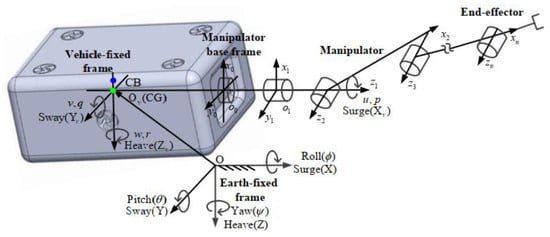
Figure 1. The coordinate frames of the UVMS.

Table 1. Nomenclature for the underwater vehicle.

Variable	Definition
$x$	X translation (Surge position)
$y$	Y translation (Sway position)
$z$	Z translation (Heave position)
$\varphi$	Rotation about X (Roll angle)
$\theta$	Rotation about Y (Pitch angle)
$\psi$	Rotation about Z (Yaw angle)

To describe the motion of the vehicle in detail, its velocity in the vehicle-fixed frame is defined as $\mathbf{\nu }={[{\mathbf{\nu }}_1^T,{\mathbf{\nu }}_2^T]}^T\in {\mathbb{R}}^6$. The vectors ${\mathbf{\nu }}_1={[u,v,w]}^T$ and ${\mathbf{\nu }}_2={[p,q,r]}^T$ are the linear velocity and angular velocity of the vehicle with respect to the Earth-fixed frame expressed in the vehicle-fixed frame, respectively. The above velocity vectors satisfy the following equations:

$${\mathbf{\nu }}_1={\mathsf{J}}_1({\mathit{\eta }}_2){\dot{\mathit{\eta }}}_1$$

(1)

$${\mathbf{\nu }}_2={\mathsf{J}}_2({\mathit{\eta }}_2){\dot{\mathit{\eta }}}_2$$

(2)

where ${\mathsf{J}}_1({\mathit{\eta }}_2)$ expresses the linear velocity transformation matrix from the Earth-fixed frame to the vehicle-fixed frame, satisfying:

$${\mathsf{J}}_1({\mathit{\eta }}_2)=\left[\begin{array}{ccc}c\psi c\theta & s\psi c\theta & -s\theta \\ c\psi s\theta s\varphi -s\psi c\varphi & s\psi s\theta s\varphi +c\psi c\varphi & c\theta s\varphi \\ c\psi s\theta c\varphi +s\psi s\varphi & s\psi s\theta c\varphi -c\psi s\varphi & c\theta c\varphi \end{array}\right]$$

(3)

and the angular velocity transformation matrix ${\mathsf{J}}_2({\mathit{\eta }}_2)$ is defined as:

$${\mathsf{J}}_2({\mathit{\eta }}_2)=\left[\begin{array}{ccc}1& 0& -s\theta \\ 0& c\varphi & c\theta s\varphi \\ 0& -s\varphi & c\theta c\varphi \end{array}\right]$$

(4)

where $c\cdot =\cos (\cdot )$ and $s\cdot =\sin (\cdot )$.

Define the vector $\mathit{q}={[{\mathit{q}}_1,\cdots ,{\mathit{q}}_n]}^T\in {\mathbb{R}}^n$ as the joint position coordinate of the manipulator in each link-fixed frame, and the time derivative $\dot{\mathit{q}}$ is its joint velocity vector.

Upon redefining another position vector $\mathit{\zeta }={[{\mathit{\eta }}_1^T,{\mathit{\eta }}_2^T,{\mathit{q}}^T]}^T$ and velocity vector $\mathbf{\omega }={[{\mathbf{\nu }}_1^T,{\mathbf{\nu }}_2^T,{\dot{\mathit{q}}}^T]}^T$, and combing with the above velocity relationships of Equations (1) and (2), it can be represented as follows:

$$\mathbf{\omega }=\mathsf{J}({\mathit{\eta }}_2)\dot{\mathit{\zeta }}$$

(5)

where $\mathsf{J}({\mathit{\eta }}_2)=\mathrm{diag}[\begin{array}{ccc}{\mathsf{J}}_1({\mathit{\eta }}_2)& {\mathsf{J}}_2({\mathit{\eta }}_2)& {\mathsf{I}}_{n\times n}\end{array}]$, and ${\mathsf{I}}_{n\times n}$ denotes the $n\times n$ identity matrix.

Here, the control task depends on the position and orientation of the end-effector in the Earth-fixed frame, which can be defined as ${\mathit{x}}_E$, i.e., ${\mathit{x}}_E={[{\mathit{p}}_E^T,{\mathit{\eta }}_E^T]}^T\in {\mathbb{R}}^6$, satisfying ${\mathit{x}}_E={\mathit{k}}_{ee}(\mathit{\zeta })$ shown in the Appendix A. The vectors ${\mathit{p}}_E$ and ${\mathit{\eta }}_E$ are the position and orientation coordinates of the end-effector in the Earth-fixed frame, respectively, where the vector ${\mathit{\eta }}_E$ is expressed in terms of Euler-angle form. The relationship between ${\dot{\mathit{x}}}_E$ and $\dot{\mathit{\zeta }}$ can be deduced from Appendix A, namely:

$${\dot{\mathit{x}}}_E={\mathsf{J}}_{OE}({\mathit{\eta }}_2,\mathit{q})\dot{\mathit{\zeta }}$$

(6)

Also, defining ${\dot{\mathbf{\varsigma }}}_E\in {\mathbb{R}}^6$ as the linear velocity and angle velocity coordinate of the end-effector in the Earth-fixed frame, the corresponding relationship between ${\dot{\mathbf{\varsigma }}}_E$ and $\dot{\mathit{\zeta }}$ refers to the Appendix A, satisfying:

$${\dot{\mathbf{\varsigma }}}_E={\mathsf{J}}_E({\mathit{\eta }}_2,\mathit{q})\cdot \dot{\mathit{\zeta }}$$

(7)

where ${\dot{\mathbf{\varsigma }}}_E={[{\dot{\mathit{p}}}_E^T,{\mathit{w}}_E^T]}^T$, and ${\mathit{w}}_E$ denotes the angle velocity of the end-effector in the Earth-fixed frame.

2.2. The Quaternion-Based CLIKA of the UVMS

The primary objective of the inverse kinematics is to find a suitable motion variable $\mathit{\zeta }(t)$ through a desired end-effector task ${\mathit{x}}_{E,d}={[{\mathit{p}}_{E,d}^T,{\mathit{\eta }}_{E,d}^T]}^T$, where ${\mathit{p}}_{E,d}$ and ${\mathit{\eta }}_{E,d}$ denote the desired position and orientation coordinates of the end-effector in the Earth-fixed frame, respectively.

The utilization of pseudoinverse of the Jacobian matrix in [3] is the simplest way to invert the mapping Equation (6):

$${\dot{\mathit{\zeta }}}_r={\mathsf{J}}_{OE}^{†}{\dot{\mathit{x}}}_{E,d}$$

(8)

with the pseudoinverse matrix ${\mathsf{J}}_{OE}^{†}={\mathsf{J}}_{OE}^T{({\mathsf{J}}_{OE}{\mathsf{J}}_{OE}^T)}^{-1}$.

Using the CLIKA in [3] provided by Equation (9), the reference position and orientation vector ${\mathit{\zeta }}_r(t)$ can be obtained via the desired end-effector task ${\mathit{x}}_{E,d}$, unlike the open-loop form may cause a numerical drift by integrating the velocities to find the related position and orientation:

$${\dot{\mathit{\zeta }}}_r={\mathsf{J}}_{OE}^{†}({\dot{\mathit{x}}}_{E,d}-{\mathsf{K}}_E{\mathit{e}}_E)$$

(9)

where ${\mathit{e}}_E={[{\mathit{e}}_{\mathit{p}}^T,{\mathit{e}}_{o,\mathrm{Eul}.}^T]}^T$, i.e., ${\mathit{e}}_p={\mathit{p}}_{E,r}-{\mathit{p}}_{E,d}$ and ${\mathit{e}}_{\mathbf{o},\mathrm{Eul}.}={\mathit{\eta }}_{E,r}-{\mathit{\eta }}_{E,d}$, is the reconstruction error vector. ${\mathit{p}}_{E,r}$ and ${\mathit{\eta }}_{E,r}$ denote reference position and orientation vectors of the end-effector corresponding to ${\mathit{\zeta }}_r$, satisfying ${\mathit{x}}_{E,r}={[{\mathit{p}}_{E,r}^T,{\mathit{\eta }}_{E,r}^T]}^T={\mathit{k}}_{ee}({\mathit{\zeta }}_r)$. The gain matrix ${\mathsf{K}}_E=\mathrm{diag}[{\mathsf{K}}_p,{\mathsf{K}}_o]\in {\mathbb{R}}^{6\times 6}$ is chosen to ensure the asymptotical convergence of the reconstruction error to zero, where ${\mathsf{K}}_p$, ${\mathsf{K}}_o\in {\mathbb{R}}^{3\times 3}$ are diagonal and positive definite matrices.

Remark 1.

The reference value ${\mathit{\zeta }}_r(t)$is second order differentiable.

If the task is considered as the position control of the end-effector only, its reconstruction error is simply given by the difference between the desired and the actual values. For the case of the orientation, the definition of such error is required to ensure convergence to the desired value, while involving in large numbers of computations of the related trigonometric and inverse trigonometric functions. In this paper the quaternion attitude representation is used to replace the expression of the orientation error [23], and we define ${\mathit{Q}}_d={[{\mathit{\eta }}_d,{\mathit{\epsilon }}_d^T]}^T$ and ${\mathit{Q}}_r={[{\mathit{\eta }}_r,{\mathit{\epsilon }}_r^T]}^T$ as the desired and reference attitudes expressed by quaternions, respectively. The quaternion-based CLIKA can be redefined as:

$${\dot{\mathit{\zeta }}}_r={\mathsf{J}}_E^{†}({\dot{\mathit{\varsigma }}}_{E,d}-{\mathsf{K}}_E{\overline{\mathit{e}}}_E)$$

(10)

along with ${\dot{\mathit{\varsigma }}}_{E,d}={[{\dot{\mathit{p}}}_{E,d}^T,{\mathit{w}}_{E,d}^T]}^T$ satisfying:

$${\mathit{w}}_{E,d}={\mathsf{J}}_3({\mathit{\eta }}_{E,d}){\dot{\mathit{\eta }}}_{E,d}$$

(11)

where ${\mathsf{J}}_3(\cdot )$ can be found in the Appendix A. Another reconstruction error is ${\overline{\mathit{e}}}_E={[{\mathit{e}}_p^T,{\mathit{e}}_{o,\mathrm{Quat}.}^T]}^T$ satisfying ${\mathit{e}}_p={\mathit{p}}_{E,r}-{\mathit{p}}_{E,d}$ and ${\mathit{e}}_{o,\mathrm{Quat}.}=-[{\mathit{\eta }}_r{\mathit{\epsilon }}_d-{\mathit{\eta }}_d{\mathit{\epsilon }}_r-\mathsf{S}({\mathit{\epsilon }}_d){\mathit{\epsilon }}_r]$, where $\mathsf{S}(\cdot )$ denotes the skew symmetric matrix of the vector. Figure 2 presents the computation process of the quaternion-based CLIKA of the UVMS. And, the output of the inverse kinematics is the reference position and orientation of the UVMS expressed by ${\mathit{\zeta }}_r(t)$, which can be taken as the tracking objective for the design of the dynamic control strategy.

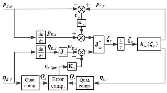
Figure 2. The quaternion-based CLIKA of the UVMS.

2.3. The Dynamics of the UVMS

Considering that the $6+n$ DOF UVMS contains a six DOF vehicle coupled with a general $n$ DOF underwater manipulator. Its dynamic equations in the vehicle-fixed frame can be derived by resorting to the Quasi-Lagrange approach [24] and expressed in the following form:

$$\mathsf{M}(\mathit{q})\dot{\mathit{\omega }}+\mathsf{C}(\mathit{q},\mathit{\omega })\mathit{\omega }+\mathbf{D}(\mathit{q},\mathit{\omega })\mathit{\omega }+\mathit{G}({\mathit{\eta }}_2,\mathit{q})+{\mathit{\tau }}_d=\mathit{\tau }$$

(12)

where $\mathsf{M}(\mathit{q})\in {\mathbb{R}}^{(6+n)\times (6+n)}$ is the inertia matrix and $\mathsf{C}(\mathit{q},\mathit{\omega })\in {\mathbb{R}}^{(6+n)\times (6+n)}$ is the centrifugal and Coriolis matrix, and both of them contain their corresponding added mass terms. $\mathbf{D}(\mathit{q},\mathit{\omega })\in {\mathbb{R}}^{(6+n)\times (6+n)}$ is the drag matrix. $\mathit{G}({\mathit{\eta }}_2,\mathit{q})\in {\mathbb{R}}^{(6+n)\times 1}$ denotes the restoring force/moment vector caused by both gravity and buoyancy effects. ${\mathit{\tau }}_d\in {\mathbb{R}}^{(6+n)\times 1}$ is the unknown external disturbance vector. And, $\mathit{\tau }\in {\mathbb{R}}^{(6+n)\times 1}$ represents the input force and moment vector acting on the UVMS. By the use of the velocity relationship in Equation (5), the dynamic equations of the UVMS in Equation (12) can be transformed into the Earth-fixed frame and rewritten as:

$${\mathsf{M}}_{\zeta }(\mathit{\zeta })\ddot{\mathit{\zeta }}+{\mathsf{C}}_{\zeta }(\mathit{\zeta },\dot{\mathit{\zeta }})\dot{\mathit{\zeta }}+{\mathbf{D}}_{\zeta }(\mathit{\zeta },\dot{\mathit{\zeta }})\dot{\mathit{\zeta }}+{\mathit{G}}_{\zeta }(\mathit{\zeta })+{\mathit{\tau }}_{\zeta ,d}={\mathit{\tau }}_{\zeta }$$

(13)

where ${\mathsf{M}}_{\zeta }(\mathit{\zeta })={\mathsf{J}}^T\mathsf{M}(\mathit{q})\mathsf{J}$, ${\mathsf{C}}_{\zeta }(\mathit{\zeta },\dot{\mathit{\zeta }})={\mathsf{J}}^T(\mathsf{C}(\mathit{q},\mathit{\omega })+\mathsf{M}(\mathit{q})\dot{\mathsf{J}}{\mathsf{J}}^{-1})\mathsf{J}$, ${\mathbf{D}}_{\zeta }(\mathit{\zeta },\dot{\mathit{\zeta }})={\mathsf{J}}^T\mathbf{D}(\mathit{q},\mathit{\omega })\mathsf{J}$, ${\mathit{G}}_{\zeta }(\mathit{\zeta })={\mathsf{J}}^T\mathit{G}({\mathit{\eta }}_2,\mathit{q})$, ${\mathit{\tau }}_{\zeta ,d}={\mathsf{J}}^T{\mathit{\tau }}_d$ and ${\mathit{\tau }}_{\zeta }={\mathsf{J}}^T\mathit{\tau }$.

Since the external environment, like ocean currents, has significant influence on the UVMS, the relevant term can be incorporated into the dynamic equations of the system.

Define the relative velocity in the Earth-fixed frame as ${\dot{\mathit{\zeta }}}_c=\dot{\mathit{\zeta }}-{\mathbf{\nu }}_c$, where ${\mathbf{\nu }}_c$ denotes the current velocity.

Remark 2 [25].

Suppose that the current velocity is irrotational and constant in the Earth-fixed frame, and it can be expanded to the $6+n$ dimensional generalized space, namely:

$${\mathbf{\nu }}_c={[{\mathbf{\nu }}_{c,x},{\mathbf{\nu }}_{c,y},{\mathbf{\nu }}_{c,z},0,\cdots ,\mathrm{upto}(6+n)]}^T\in {\mathbb{R}}^{(6+n)\times 1}$$

(14)

Substituting $\dot{\mathit{\zeta }}$ in Equation (13) with ${\dot{\mathit{\zeta }}}_c$, the dynamic equations of the UVMS under current effect can be represented as:

$${\mathsf{M}}_{\zeta }(\mathit{\zeta })\ddot{\mathit{\zeta }}+{\mathsf{C}}_{\zeta }(\mathit{\zeta },{\dot{\mathit{\zeta }}}_c){\dot{\mathit{\zeta }}}_c+{\mathbf{D}}_{\zeta }(\mathit{\zeta },{\dot{\mathit{\zeta }}}_c){\dot{\mathit{\zeta }}}_c+{\mathit{G}}_{\zeta }(\mathit{\zeta })+{\mathit{\tau }}_{\zeta ,\mathbf{d}}={\mathit{\tau }}_{\zeta }$$

(15)

Moreover, the terms related to ${\mathbf{\nu }}_c$ in Equation (15) can be combined as a new vector ${\mathit{\tau }}_c(\mathit{\zeta },\dot{\mathit{\zeta }},{\mathbf{\nu }}_c)$. Hence, the dynamic equations of the UVMS under current effect takes the form:

$${\mathsf{M}}_{\zeta }(\mathit{\zeta })\ddot{\mathit{\zeta }}+{\mathsf{C}}_{\zeta }(\mathit{\zeta },\dot{\mathit{\zeta }})\dot{\mathit{\zeta }}+{\mathbf{D}}_{\zeta }(\mathit{\zeta },\dot{\mathit{\zeta }})\dot{\mathit{\zeta }}+{\mathit{G}}_{\zeta }(\mathit{\zeta })+{\mathit{\tau }}_c(\mathit{\zeta },\dot{\mathit{\zeta }},{\mathbf{\nu }}_c)+{\mathit{\tau }}_{\zeta ,\mathbf{d}}={\mathit{\tau }}_{\zeta }$$

(16)

It is noted that the UVMS can be influenced by uncertain factors such as parameter uncertainties, hydrodynamics and external disturbances, the system dynamic equations in Equation (16) can be rewritten as:

$$({\widehat{\mathsf{M}}}_{\zeta }+\Delta {\mathsf{M}}_{\mathit{\zeta }})\ddot{\mathit{\zeta }}+({\widehat{\mathsf{C}}}_{\zeta }+\Delta {\mathsf{C}}_{\zeta })\dot{\mathit{\zeta }}+({\widehat{\mathbf{D}}}_{\zeta }+\Delta {\mathbf{D}}_{\zeta })\dot{\mathit{\zeta }}+({\widehat{\mathit{G}}}_{\zeta }+\Delta {\mathit{G}}_{\zeta })+{\mathit{\tau }}_c(\mathit{\zeta },\dot{\mathit{\zeta }},{\mathbf{\nu }}_c)+{\mathit{\tau }}_{\zeta ,d}={\mathit{\tau }}_{\zeta }$$

(17)

For the convenience of the subsequent analysis, the dynamic equations illustrated by Equation (17) can be transformed into the following form:

$$\ddot{\mathit{\zeta }}=\mathit{F}(t)+\mathit{d}(t)+{\widehat{\mathsf{M}}}_{\zeta }^{-1}\cdot {\mathit{\tau }}_{\zeta }$$

(18)

where $\mathit{F}(t)$ and $\mathit{d}(t)$ are defined as nominal model term and the lumped disturbance vector of the system, respectively, and given by:

$$\{\begin{array}{l}\mathit{F}(t)=-{\widehat{\mathsf{M}}}_{\zeta }^{-1}({\widehat{\mathsf{C}}}_{\zeta }\dot{\mathit{\zeta }}+{\widehat{\mathbf{D}}}_{\zeta }\dot{\mathit{\zeta }}+{\widehat{\mathit{G}}}_{\zeta })\\ \mathbf{d}(t)=-{\widehat{\mathsf{M}}}_{\zeta }^{-1}(\Delta {\mathsf{M}}_{\zeta }\ddot{\mathit{\zeta }}+\Delta {\mathsf{C}}_{\zeta }\dot{\mathit{\zeta }}+\Delta {\mathbf{D}}_{\zeta }\dot{\mathit{\zeta }}+\Delta {\mathit{G}}_{\zeta }+{\mathit{\tau }}_c(\mathit{\zeta },\dot{\mathit{\zeta }},{\mathbf{\nu }}_c))+{\mathit{d}}_{\zeta }\end{array}$$

(19)

where ${\mathit{d}}_{\zeta }=-{\widehat{\mathsf{M}}}_{\zeta }^{-1}\cdot {\mathit{\tau }}_{\zeta ,d}$ denotes the disturbance term related to the external disturbances.

Assumption 1.

The time derivative of the lumped disturbance vector defined as $\dot{\mathit{d}}(t)$is bounded by $L_d$, i.e.,${\Vert \dot{\mathit{d}}(t)\Vert }_1\le L_d$, where the upper bound $L_d$is a positive constant.

2.4. Notation and Lemmas

In this section, some notations are defined: for any $\mathit{x}={[{\mathit{x}}_1,\cdots ,{\mathit{x}}_n]}^T\in {\mathbb{R}}^n$, ${\mathit{x}}_i\in \mathbb{R}$, $\mathit{\alpha }={[{\mathit{\alpha }}_1,\cdots ,{\mathit{\alpha }}_n]}^T\in {\mathbb{R}}_{+}^n$, ${\mathit{\alpha }}_i\in {\mathbb{R}}_{+}$, $i=1,\cdots ,n$, ${\Vert \mathit{x}\Vert }_1={\displaystyle {\sum }_{i=1}^n\left|{\mathit{x}}_i\right|}$ and ${\Vert \mathit{x}\Vert }_2=\sqrt{{{\displaystyle {\sum }_{i=1}^n\left|{\mathit{x}}_i\right|}}^2}$ denote the 1-norm and 2-norm of the vector $\mathit{x}$, respectively; consider $\mathrm{sig}{({\mathit{x}}_1)}^{{\mathit{\alpha }}_1}={\left|{\mathit{x}}_1\right|}^{{\mathit{\alpha }}_1}\cdot \mathrm{sign}({\mathit{x}}_1)$ where $\mathrm{sign}(\cdot )$ represents the signum function, and define $\mathrm{sig}{(\mathit{x})}^{{\mathit{\alpha }}_1}={[\mathrm{sig}{({\mathit{x}}_1)}^{{\mathit{\alpha }}_1},\cdots ,\mathrm{sig}{({\mathit{x}}_n)}^{{\mathit{\alpha }}_1}]}^T$ and $\mathrm{sig}{(\mathit{x})}^{\mathit{\alpha }}={[\mathrm{sig}{({\mathit{x}}_1)}^{{\mathit{\alpha }}_1},\cdots ,\mathrm{sig}{({\mathit{x}}_n)}^{{\mathit{\alpha }}_n}]}^T$.

Lemma 1 [26]. 

Let $k_1,\cdots ,k_n>0$such that the polynomial $s^n+k_n{s}^{n-1}+\cdots +k_{2}s+k_1$is Hurwitz, and considerthe system ${\dot{x}}_1=x_2,\cdots ,{\dot{x}}_{n-1}=x_n,{\dot{x}}_n=u(t)$. There existssufficiently small $\vartheta \in (0,1)$such that, for every $\alpha \in (1-\vartheta ,1)$, the system can realize the globally finite-time stability under the feedback $u(t)=-k_1 \cdot \mathrm{sig}{(x_1)}^{{\alpha }_1}-\cdots -k_n\cdot \mathrm{sig}{(x_n)}^{{\alpha }_n}$, where ${\alpha }_i$, $i=1,\cdots ,n$, satisfy the recurrent relations ${\alpha }_{i-1}={\alpha }_i{\alpha }_{i+1}/(2{\alpha }_{i+1}-{\alpha }_i)$, $i=1,\cdots ,n$, with ${\alpha }_{n+1}=1$and ${\alpha }_n=\alpha$.

Lemma 2 [27].

If a bounded signal is square integrable and also has a bounded first order time derivative, the signal can converge to zero asymptotically.

3. Control Strategy

Define the position tracking error vector ${\mathit{e}}_1$ and its time derivative ${\dot{\mathit{e}}}_1$ satisfying ${\mathit{e}}_1=\mathit{\zeta }-{\mathit{\zeta }}_r$ and ${\mathit{z}}_1={\dot{\mathit{e}}}_1=\dot{\mathit{\zeta }}-{\dot{\mathit{\zeta }}}_r$. The objective is to design a suitable control scheme that can make the position tracking error vector ${\mathit{e}}_1$ achieve the asymptotical convergence to zero.

3.1. NFTSMC

Let us define an auxiliary term ${\mathit{z}}_2$ in the following:

$${\mathit{z}}_2={\mathit{z}}_1+{\mathsf{C}}_1{\displaystyle {\int }_0^t\mathrm{sig}{({\mathit{e}}_1)}^{{\alpha }_1}dt}+{\mathsf{C}}_2{\displaystyle {\int }_0^t\mathrm{sig}{({\mathit{z}}_1)}^{{\alpha }_2}dt}$$

(20)

and then, to achieve the fast convergence and avoid singularity, the modified NFTSMS variable $\mathit{s}$ is designed as follows under the inspiration of both [26,28]:

$$\mathit{s}={\mathit{z}}_2+{\mathsf{C}}_3{\displaystyle {\int }_0^t\mathrm{sig}{({\mathit{z}}_2)}^{{\alpha }_3}dt}+{\mathsf{C}}_4{\displaystyle {\int }_0^t\mathrm{sig}{({\mathit{z}}_2)}^{{\beta }_1}dt}$$

(21)

where the gain matrices ${\mathsf{C}}_i=\mathrm{diag}[{\mathit{c}}_{i1},\cdots ,{\mathit{c}}_{i,6+n}]$, $i=1,2,3,4$, have their components satisfying ${\mathit{c}}_{ij}>0$, $i=1,2,3,4$, $j=1,\cdots ,6+n$. The constant parameter vectors ${\mathit{\alpha }}_h$, $h=1,2,3$, and ${\mathit{\beta }}_1$ are defined as ${\mathit{\alpha }}_h={[{\mathit{\alpha }}_{h1},\cdots ,{\mathit{\alpha }}_{h,6+n}]}^T$, $h=1,2,3$, and ${\mathit{\beta }}_1={[{\mathit{\beta }}_{11},\cdots ,{\mathit{\beta }}_{1,6+n}]}^T$, respectively. Besides, the components of the matrices ${\mathsf{C}}_1$ and ${\mathsf{C}}_2$, and the vector ${\mathit{\alpha }}_1$ and ${\mathit{\alpha }}_2$ are selected based on Lemma 1, i.e., the Hurwitz polynomials ${\mathit{s}}^2+{\mathbf{c}}_{2j}\mathit{s}+{\mathbf{c}}_{1j}$, $j=1,\cdots ,6+n$ and ${\mathit{\alpha }}_{1j}={\mathit{\alpha }}_{2j}/(2-{\mathit{\alpha }}_{2j})$, $j=1,\cdots ,6+n$ with existing a small constant ${\vartheta }_1\in (0,1)$ s.t. ${\mathit{\alpha }}_{2j}\in (1-{\vartheta }_1,1)$. Next, the constant parameter vectors ${\mathit{\alpha }}_3$ and ${\mathit{\beta }}_1$ are chosen in accordance with [28], satisfying ${\mathit{\alpha }}_{3j}\in (0,1)$ and ${\mathit{\beta }}_{1j}\in [1,+\infty )$, $j=1,\cdots ,6+n$.

Considering the situation when the sliding mode variable $\mathit{s}$ reaches the sliding switched surface, namely, $\mathit{s}(t)=0$, it can also result $\dot{\mathit{s}}(t)=0$. By the use of Equation (21), we can derive:

$${\dot{\mathit{z}}}_2+{\mathbf{C}}_3\mathrm{sig}{({\mathit{z}}_2)}^{{\mathit{\alpha }}_3}+{\mathbf{C}}_4\mathrm{sig}{({\mathit{z}}_2)}^{{\mathit{\beta }}_1}=0$$

(22)

Through Definition 2 in [28], it concludes from Equation (22) that the auxiliary vector ${\mathit{z}}_2$ can converge to the origin in finite time. That is, there exists $T_1$ such that ${\mathit{z}}_2=0$ holds for all $t\ge T_1$, which can further imply ${\dot{\mathit{z}}}_2=0$. Based on this, combining with Equation (20), it yields:

$${\dot{\mathit{z}}}_1+{\mathbf{C}}_1\mathrm{sig}{({\mathit{e}}_1)}^{{\mathit{\alpha }}_1}+{\mathbf{C}}_2\mathrm{sig}{({\mathit{z}}_1)}^{{\mathit{\alpha }}_2}=0$$

(23)

By using ${\mathit{z}}_1={\dot{\mathit{e}}}_1$ and Lemma 1, it can deduce that the position tracking error vector ${\mathit{e}}_1$ can achieve the convergence to zero in finite time.

Upon introducing another auxiliary term:

$${\mathit{z}}_0={\mathbf{C}}_1{\displaystyle {\int }_0^t\mathrm{sig}{({\mathit{e}}_1)}^{{\mathit{\alpha }}_1}dt}+{\mathbf{C}}_2{\displaystyle {\int }_0^t\mathrm{sig}{({\mathit{z}}_1)}^{{\mathit{\alpha }}_2}dt}$$

(24)

and then Equation (20) can be also expressed as ${\mathit{z}}_2={\mathit{z}}_1+{\mathit{z}}_0$.

3.2. ESO

Taking the lumped disturbance vector $\mathit{d}(t)$ as an extended state, and combining with (24), the extended dynamic form of Equation (19) can be expressed as:

$$\{\begin{array}{l}{\dot{\mathit{z}}}_2=\mathit{F}(t)-{\ddot{\mathit{\zeta }}}_r+{\dot{\mathit{z}}}_0+{\widehat{\mathsf{M}}}_{\zeta }^{-1}\cdot {\mathit{\tau }}_{\zeta }+\mathit{d}\\ \dot{\mathit{d}}=\mathit{h}(t)\end{array}$$

(25)

where $\mathit{h}(t)$ denotes the time derivative of the lumped disturbance vector $\mathit{d}(t)$.

The fixed-time convergent ESO is designed referring to [22]. To avoid the chattering due to the discontinuous signum function, $\mathrm{sign} (\cdot )$ in the ESO is replaced by a saturation function $\mathrm{sat} (\cdot )$. The modified ESO can be represented:

$$\{\begin{array}{l}{\dot{\widehat{\mathit{z}}}}_2=\mathit{F}(t)-{\ddot{\mathit{\zeta }}}_r+{\dot{\mathit{z}}}_0+{\widehat{\mathsf{M}}}_{\mathit{\zeta }}^{-1}\cdot {\mathit{\tau }}_{\mathit{\zeta }}+{\rho }_1\cdot \mathrm{sig}{({\tilde{\mathit{z}}}_2)}^{1/2}+{\rho }_2\cdot \mathrm{sig}{({\tilde{\mathit{z}}}_2)}^{{\gamma }_1}+\widehat{\mathit{d}}\\ \dot{\widehat{\mathit{d}}}={\rho }_3\cdot \mathrm{sat}({\tilde{\mathit{z}}}_2)\end{array}$$

(26)

where the constant gain parameters satisfy ${\rho }_1$, ${\rho }_2$, ${\rho }_3>0$ and ${\gamma }_1>1$. The vectors ${\widehat{\mathit{z}}}_2$ and $\widehat{\mathit{d}}$ denote the estimation values of the state vector ${\mathit{z}}_2$ and $\mathit{d}$, respectively. And, the vector ${\tilde{\mathit{z}}}_2$ is the estimation error of the state vector ${\mathit{z}}_2$, i.e., ${\tilde{\mathit{z}}}_2={\mathit{z}}_2-{\widehat{\mathit{z}}}_2$ with its component form ${\tilde{\mathit{z}}}_2={[{\tilde{\mathit{z}}}_{21},\cdots ,{\tilde{\mathit{z}}}_{2,6+n}]}^T$. Meanwhile, the saturation function $\mathrm{sat}({\tilde{\mathit{z}}}_2)$ is defined as:

$$\mathrm{sat}({\tilde{z}}_{2j})=\{\begin{array}{l}\tanh ({\tilde{z}}_{2j}/{\epsilon }_{1j}) \mathrm{for}\left|{\tilde{z}}_{2j}\right|\le {\epsilon }_{1j} j=1,\cdots ,6+n\\ \mathrm{sign}({\tilde{z}}_{2j}) \mathrm{for}\left|{\tilde{z}}_{2j}\right|>{\epsilon }_{1j} j=1,\cdots ,6+n\end{array}$$

(27)

Remark 3.

Choose the saturation function instead of the conventional sign function, and it can attenuate the chattering caused by the latter discontinuity.

Combining Equations (25) and (26), the estimation error equation for the ESO can be expressed as:

$$\{\begin{array}{l}{\dot{\tilde{\mathit{z}}}}_2=-{\rho }_1\cdot \mathrm{sig}{({\tilde{\mathit{z}}}_2)}^{1/2}-{\rho }_2\cdot \mathrm{sig}{({\tilde{\mathit{z}}}_2)}^{{\gamma }_1}+\tilde{\mathit{d}}\\ \dot{\tilde{\mathit{d}}}=-{\rho }_3\cdot \mathrm{sat}({\tilde{\mathit{z}}}_2)+\mathit{h}(t)\end{array}$$

(28)

where $\tilde{\mathit{d}}=\mathit{d}-\widehat{\mathit{d}}$ denotes the estimation error of the lumped disturbance vector $\mathit{d}$.

The result follows from Theorem 2 in [22] that both the estimation errors ${\tilde{\mathit{z}}}_2$ and $\tilde{\mathit{d}}$ can converge to the origin uniformly in fixed time.

3.3. Adaptive Control Law

An adaptive control scheme can be proposed for the trajectory tracking control of the UVMS subjected to the lumped disturbances.

Assumption 2.

The disturbance estimation error satisfies ${\Vert \tilde{\mathit{d}}\Vert }_1\le \delta$where the upper bound $\delta$is unknown.

Theorem 1.

Considering the dynamic equations of the UVMS in Equation (19), and combing the ESO in Equation (26) under Assumptions 1–2, the proposed control law can be chosen as:

$${\mathit{\tau }}_{\mathit{\zeta }}={\widehat{\mathsf{M}}}_{\mathit{\zeta }}\cdot [-(\mathit{F}(t)-{\ddot{\mathit{\zeta }}}_r+{\dot{\mathit{z}}}_0+{\mathbf{C}}_3\mathrm{sig}{({\mathit{z}}_2)}^{{\alpha }_3}+{\mathbf{C}}_4\mathrm{sig}{({\mathit{z}}_2)}^{{\beta }_1})-\widehat{\mathit{d}}-{\mathsf{K}}_1\cdot \mathit{s}-{\mathit{u}}_r]$$

(29)

where ${\mathsf{K}}_1=\mathrm{diag}[k_{11},\cdots ,k_{1,6+n}]$ is the gain matrix with its components satisfying $k_{1j}>0$, $j=1,\cdots ,6+n$. The conventional robust term in Equation (29) is defined as:

$${\mathit{u}}_r=\widehat{\delta }\cdot \mathrm{sign}(\mathit{s})$$

(30)

where $\widehat{\delta }$ presenting the estimation value of the parameter $\delta$ is calculated by the following adaptive law:

$$\dot{\widehat{\delta }}={\rho }_4\cdot {\Vert \mathit{s}\Vert }_1$$

(31)

Thus, all of the related state signals like $\mathit{s}$ and $\tilde{\delta }$ are bounded, and the position tracking error vector of the system ${\mathit{e}}_1$ can converge to zero asymptotically.

Proof of Theorem 1.

Considering the following Lyapunov function that is positive and define:

$$V_1={\mathit{s}}^T\cdot \mathit{s}/2+{\tilde{\delta }}^2/(2{\rho }_4)$$

(32)

where $\tilde{\delta }=\delta -\widehat{\delta }$ is the estimation error of the parameter $\delta$.

With respect to combining the above Equations (21), (25), (29)–(31), the time derivative of $V_1$ yields:

$$\begin{array}{l}{\dot{V}}_1={\mathit{s}}^T\cdot \dot{\mathit{s}}+\tilde{\delta }\cdot \dot{\tilde{\delta }}/{\rho }_4\\ ={\mathit{s}}^T\cdot [\mathit{F}(t)-{\ddot{\mathit{\zeta }}}_r+{\dot{\mathit{z}}}_0+{\mathbf{C}}_3\mathrm{sig}{({\mathit{z}}_2)}^{{\alpha }_3}+{\mathbf{C}}_4\mathrm{sig}{({\mathit{z}}_2)}^{{\beta }_1}+{\widehat{\mathsf{M}}}_{\zeta }^{-1}\cdot {\mathit{\tau }}_{\zeta }+\mathit{d}]-\tilde{\delta }\cdot \dot{\widehat{\delta }}/{\rho }_4\\ ={\mathit{s}}^T\cdot (\tilde{\mathit{d}}-{\mathsf{K}}_1\cdot \mathit{s}-\widehat{\delta }\cdot \mathrm{sign}(\mathit{s}))-\tilde{\delta }\cdot {\Vert \mathit{s}\Vert }_1\\ \le {\Vert \tilde{\mathit{d}}\Vert }_1\cdot {\Vert \mathit{s}\Vert }_1-{\mathit{s}}^T{\mathsf{K}}_1\mathit{s}-\widehat{\delta }\cdot {\Vert \mathit{s}\Vert }_1-\tilde{\delta }\cdot {\Vert \mathit{s}\Vert }_1\\ =-{\mathit{s}}^T{\mathsf{K}}_1\mathit{s}-(\delta -{\Vert \tilde{\mathit{d}}\Vert }_1)\cdot {\Vert \mathit{s}\Vert }_1\\ \le -{\mathit{s}}^T{\mathsf{K}}_1\mathit{s}\\ \le -{\lambda }_1{\mathit{s}}^T\mathit{s}\end{array}$$

(33)

where ${\lambda }_1={\lambda }_{\mathbf{min}}({\mathsf{K}}_1)$, and ${\lambda }_{\mathbf{min}}(\cdot )$ denotes the minimum eigenvalue of the matrix.

According to Equation (33), we can obtain ${\dot{V}}_1\le -{\lambda }_1{\mathit{s}}^T\mathit{s}$ all the time, so the inequality relation ${\dot{V}}_1<0$ holds for every $\mathit{s}\ne 0$, which further demonstrates that the signals like $V_1$, $\mathit{s}$ and $\tilde{\delta }$ are bounded. From the above derivation, we have:

$$\dot{\mathit{s}}=\tilde{\mathit{d}}-{\mathsf{K}}_1\cdot \mathit{s}-\widehat{\delta }\cdot \mathrm{sign}(\mathit{s})$$

(34)

For the reason that the vectors $\mathit{s}$ and $\tilde{\delta }$ are bounded, in combination with the Assumption 2, we know that the estimation value $\widehat{\delta }$ is bounded. Furthermore, it can conclude the boundness of $\dot{\mathit{s}}$. Introducing another new function $L_1(\mathit{s})={\lambda }_1{\mathit{s}}^T\mathit{s}$, both $L_1(\mathit{s})$ and its time derivative are bounded because of the boundness of the vectors $\mathit{s}$ and $\dot{\mathit{s}}$. Then, we can obtain $\underset{T\to \infty }{\mathbf{lim}}{\displaystyle {\int }_0^t{L}_1(\mathit{s})}\le V_1(0)-V_1(\infty )$. Since both $V_1(0)$ and $V_1(\infty )$ are bounded, the sliding mode variable $\mathit{s}$ is square integrable. Hence, the function $L(\mathit{s})$ can converge to zero asymptotically via Lemma 2, which further derives the asymptotical convergence of the sliding mode variable $\mathit{s}$ to zero. Finally, in accordance with the above Equation (21), it results that the position tracking error vector ${\mathit{e}}_1$ can achieve the asymptotical convergence to zero.

As the conventional robust term in Equation (30) contains the discontinuous signum function, it may cause the chattering problem. Inspired by [26,29], a continuous fractional PI-type controller is designed as:

$${\mathit{u}}_r(\mathit{s}|\mathit{\chi })={\mathit{\chi }}^T\cdot \mathit{\phi }(\mathit{s})$$

(35)

where $\mathit{\chi }={[\begin{array}{cc}{\mathit{\chi }}_1& {\mathit{\chi }}_2\end{array}]}^T$ and $\mathit{\phi }(\mathit{s})={[\begin{array}{cc}\mathit{s}& {\displaystyle {\int }_0^t\mathrm{sig}{(\mathit{s})}^{{\alpha }_4}dt}\end{array}]}^T$, ${\mathit{\alpha }}_4\in (0,1)$. According to the analysis found in [29], we can use ${\mathit{u}}_r(\mathit{s}|\widehat{\mathit{\chi }})$ to approximate the conventional robust term ${\mathit{u}}_r=\widehat{\delta }\mathrm{sign}(\mathit{s})$, and the related estimated value $\widehat{\mathit{\chi }}$ can be derived from Lyapunov theory. Consequently, we can get the modified control scheme based on Equation (35) shown in the following Theorem 2. □

Theorem 2.

Consider the dynamic equations of the UVMS described by Equation (19) satisfying Assumptions 1–2. In combination with the ESO in Equation (26), the control law of the system is determined by Equation (29), satisfying the continuous fractional PI-type robust term in Equation (36) and the adaptive laws in Equations (31) and (37):

$${\mathit{u}}_r(\mathit{s}|\widehat{\mathit{\chi }})={\widehat{\mathit{\chi }}}^T\cdot \mathit{\phi }(\mathit{s})$$

(36)

$$\dot{\widehat{\mathit{\chi }}}={\rho }_5\cdot \mathit{\phi }(\mathit{s})\cdot \mathit{s}$$

(37)

Thus, all of the related state signals such as $\mathit{s}$, $\tilde{\delta }$, and $\tilde{\mathit{\chi }}$ are bounded, and the position tracking error vector of the system ${\mathit{e}}_1$ can achieve the asymptotical convergence to zero.

Proof of Theorem 2.

Choosing another positive definite Lyapunov function is expressed as:

$$V_2={\mathit{s}}^T\cdot \mathit{s}/2+{\tilde{\delta }}^2/(2{\rho }_4)+\mathrm{tr}({\tilde{\mathit{\chi }}}^T\cdot \tilde{\mathit{\chi }})/(2{\rho }_5)$$

(38)

where $\tilde{\mathit{\chi }}={\mathit{\chi }}^{\ast }-\widehat{\mathit{\chi }}$ is the estimation error of $\mathit{\chi }$ and its optimal value ${\mathit{\chi }}^{\ast }$ is defined as:

$${\mathit{\chi }}^{\ast }=\arg \underset{\mathit{\chi }\in {\mathbb{R}}^{2(6+n)\times (6+n)}}{\min }\left[\underset{\mathit{s}\in {\mathbb{R}}^{(6+n)\times 1}}{\sup }\left|{\mathit{u}}_r(\mathit{s}|\mathit{\chi })-\widehat{\delta }\cdot \mathrm{sign}(\mathit{s})\right|\right]$$

(39)

Combining with Equations (29), (31), (36)–(37), the time derivative of $V_2$ yields:

$$\begin{array}{l}{\dot{V}}_2={\mathit{s}}^T\cdot \dot{\mathit{s}}+\tilde{\delta }\cdot \dot{\tilde{\delta }}/{\rho }_4+\mathrm{tr}({\tilde{\mathit{\chi }}}^T\cdot \dot{\tilde{\mathit{\chi }}})/{\rho }_5\\ ={\mathit{s}}^T(\tilde{\mathit{d}}-{\mathsf{K}}_1\cdot \mathit{s}-{\mathit{u}}_r(\mathit{s}|\widehat{\mathit{\chi }}))-\tilde{\delta }\cdot \dot{\widehat{\delta }}/{\rho }_4-\mathrm{tr}({\tilde{\mathit{\chi }}}^T\cdot \dot{\widehat{\mathit{\chi }}})/{\rho }_5\\ ={\mathit{s}}^T(\tilde{\mathit{d}}-{\mathsf{K}}_1\cdot \mathit{s}-{\mathit{u}}_r(\mathit{s}|\widehat{\mathit{\chi }})+{\mathit{u}}_r(\mathit{s}|{\mathit{\chi }}^{\ast })-{\mathit{u}}_r(\mathit{s}|{\mathit{\chi }}^{\ast }))-\tilde{\delta }\cdot \dot{\widehat{\delta }}/{\rho }_4-\mathrm{tr}({\tilde{\mathit{\chi }}}^T\cdot \dot{\widehat{\mathit{\chi }}})/{\rho }_5\\ ={\mathit{s}}^T(\tilde{\mathit{d}}-{\mathsf{K}}_1\cdot \mathit{s}+{\tilde{\mathit{\chi }}}^T\cdot \mathit{\phi }(\mathit{s})-{\mathit{u}}_r(\mathit{s}|{\mathit{\chi }}^{\ast }))-\tilde{\delta }\cdot \dot{\widehat{\delta }}/{\rho }_4-\mathrm{tr}({\tilde{\mathit{\chi }}}^T\cdot \dot{\widehat{\mathit{\chi }}})/{\rho }_5\\ =-{\mathit{s}}^T{\mathsf{K}}_1\mathit{s}+{\mathit{s}}^T\cdot (\tilde{\mathit{d}}-{\mathit{u}}_r(\mathit{s}|{\mathit{\chi }}^{\ast }))-\tilde{\delta }\cdot {\Vert \mathit{s}\Vert }_1+\mathrm{tr}({\tilde{\mathit{\chi }}}^T\cdot (\mathit{\phi }(\mathit{s})\cdot \mathit{s}-\dot{\widehat{\mathit{\chi }}}/{\rho }_5))\\ \le -{\mathit{s}}^T{\mathsf{K}}_1\mathit{s}+{\Vert \mathit{s}\Vert }_1\cdot {\Vert \tilde{\mathit{d}}\Vert }_1-\widehat{\delta }\cdot {\Vert \mathit{s}\Vert }_1-\tilde{\delta }\cdot {\Vert \mathit{s}\Vert }_1\\ =-{\mathit{s}}^T{\mathsf{K}}_1\mathit{s}-(\delta -{\Vert \tilde{\mathit{d}}\Vert }_1)\cdot {\Vert \mathit{s}\Vert }_1\\ \le -{\mathit{s}}^T{\mathsf{K}}_1\mathit{s}\end{array}$$

(40)

Similarly, it can conclude from Equation (40) that ${\dot{V}}_2\le 0$ holds for any $\mathit{s}\in {\mathbb{R}}^{(6+n)\times 1}$, that is, ${\dot{V}}_2$ is negative semi-definite. Therefore, the Lyapunov function $V_2$ is bounded, which implies that the signals $\mathit{s}$, $\tilde{\delta }$ and $\tilde{\mathit{\chi }}$ are bounded. In addition that, we can obtain:

$$\dot{\mathit{s}}=\tilde{\mathit{d}}-{\mathsf{K}}_1\cdot \mathit{s}+{\tilde{\mathit{\chi }}}^T\cdot \mathit{\phi }(\mathit{s})-{\mathit{u}}_r(\mathit{s}|{\mathit{\chi }}^{\ast })$$

(41)

It is easy to know that the terms on the right of Equation (41) are bounded, thus the boundness of $\dot{\mathit{s}}$ can be ensured. According to the similar analysis in Equation (34), it can finally derive that the position tracking error vector ${\mathit{e}}_1$ can achieve the asymptotical convergence to zero. In summary, the asymptotic stability of the system can be guaranteed by the Lyapunov theory. □

Figure 3 describes the complete control process for the trajectory tracking of the UVMS. First, the quaternion-based CLIKA can be used to solve the reference position and orientation through the desired values of the UVMS end-effector. The proposed controller contains three parts: NFTSMS, ESO and adaptive control law. Combining with the position and velocity errors, the modified NFTSMS is designed to achieve the fast convergence of the tracking errors. Based on this, to estimate the lumped disturbances, the ESO method is utilized by taking the lumped disturbance vector as an extended state of the system. Meanwhile, an adaptive robust term is applied for handling the unknown boundness of the disturbance estimation errors. Then, incorporating NFTSMS, ESO and adaptive law into the control law, the obtained efforts are taken as the control inputs that can drive both vehicle and manipulator to approximate the reference values. In general, those input efforts should act on the thrust equipment of the underwater vehicle like thrusters in [30] to achieve proper operation, while it’s not the focus of this paper. The actual position and velocity as the control outputs are used to assign the related position and velocity errors. After that, the actual position information can be taken as the input of the forward kinematics to solve the actual position and orientation of the UVMS end-effector. Finally, the closed-loop control process is formed to support the following simulation.

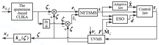
Figure 3. The adaptive NFTSMC diagram based on ESO of the UVMS.

4. Simulation

In this section, simulations with the help of MATLAB/Simulink toolbox are performed on a ten DOF UVMS, where the UVMS contains a four DOF underwater vehicle and a six DOF underwater manipulator, and its coordinated frames are shown in Figure 4. Then, some assumptions are given in the following: the gravity of the underwater vehicle equals its buoyancy; The link density of the manipulator is 2700 kg/m³, and the centre of buoyancy of the underwater manipulator is coincident with its centre of gravity; the density of the fluid is 1025.9 kg/m³; the coefficient of water resistance $C_D=1.05$; The coefficient of additional mass force is $C_M=0.8$. The dynamic parameters of the vehicle are expressed in Table 2 referring to [31,32], and its centres of gravity and buoyancy in the vehicle-fixed frame are [0, 0, 0] m and [0, 0, 0.04] m, respectively. The related link parameters of the manipulator are listed in Table 3, and the position of the base origin in the vehicle-fixed frame is [0.5, 0, 0] m.

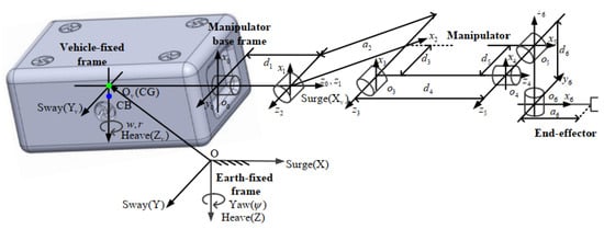
Figure 4. The coordinated frames of the ten DOF UVMS.

Table 2. The model parameters and hydrodynamic coefficients of the underwater vehicle.

Parameters	Value	Definition
$m$ (kg)	180	Mass of the vehicle
$I_z$ (kg m2)	28	Moment of inertia in z axis
$X_{\dot{u}}$,$Y_{\dot{v}}$,$Z_{\dot{w}}$ (kg)	−30, −110, −80	Add mass
$N_{\dot{r}}$ (kg m)	−1	Add mass
$X_u$,$Y_v$,$Z_w$ (kg/s)	−80, −110, −100	Linear damping
$N_r$ (kg m/s)	−10	Linear damping
$X_{u\left|u\right|}$,$Y_{v\left|v\right|}$,$Z_{w\left|w\right|}$ (kg/m)	−120, −200, −150	Crossflow drag
$N_{r\left|r\right|}$ (kg m)	−15	Crossflow drag

Table 3. The link parameters of the manipulator.

Parameters	Link 1	Link 2	Link 3	Link 4	Link 5	Link 6
${\alpha }_{i-1}$ (rad)	0	$\pi /2$	0	$\pi /2$	$-\pi /2$	$-\pi /2$
$a_{i-1}$ (m)	0	0	1.0	0	0	0
$d_i$ (m)	0.24	0	0.14	1.28	−0.14	−0.19
${\theta }_i$ (rad)	${\theta }_1$	${\theta }_2$	${\theta }_3$	${\theta }_4$	${\theta }_5$	${\theta }_6$

Assume that the desired trajectory and attitude of the UVMS end-effector can be formulated by:

$$\{\begin{array}{l}{x}_d=-2+3\cos (\pi t/25) \mathsf{m}\\ y_d=-1-5\sin (\pi t/25) \mathsf{m}\\ z_d=0.03t-0.5 \mathsf{m}\end{array} , \{\begin{array}{l}{\varphi }_d=0.2\cdot \sin (\pi t/30) \mathrm{rad}\\ {\theta }_d=0.1\cdot \cos (\pi t/30) \mathrm{rad}\\ {\psi }_d=0.15\cdot \cos (\pi t/30) \mathrm{rad}\end{array}$$

(42)

The initial position and orientation of the UVMS end-effector is (−0.09 m, 0.4 m, −1.19 m, 0 rad, 0 rad, 0 rad). And, the ten DOF UVMS is considered to be subjected to the lumped disturbances, which contain the parameter uncertainties with $\Delta {\mathsf{M}}_{\zeta } =0.1{\mathsf{M}}_{\zeta }$, $\Delta {\mathbf{C}}_{\zeta }=0.1{\mathbf{C}}_{\zeta }$, $\Delta {\mathit{d}}_{\zeta }=0.1{\mathit{d}}_{\zeta }$, and $\Delta {\mathbf{G}}_{\zeta }=0.1{\mathbf{G}}_{\zeta }$, and the velocity of the water currents with (0.1, 0.1, 0) m/s in the earth-fixed frame. In addition, provided that the unknown external disturbance vector is expressed as: $d_{\zeta 1}=0.2\sin (\pi t/15)$ m/s², $d_{\zeta 2}=0.15\cos (\pi t/15)$ m/s²,$d_{\zeta 3}=0.2\sin (\pi t/15)$ m/s², $d_{\zeta 4}=0.15\cos (\pi t/15)$ rad/s², $d_{\zeta 5}=0.1\sin (\pi t/15)$ rad/s², $d_{\zeta 6}=0.12\cos (\pi t/15)$ rad/s², $d_{\zeta 7}=0.12\sin (\pi t/15)$ rad/s², $d_{\zeta 8}=0.11\cos (\pi t/15)$ rad/s²,$d_{\zeta 9}=0.1\sin (\pi t/15)$ rad/s² and $d_{\zeta 10}=0.1\cos (\pi t/15)$ rad/s². Then, the control strategies for the first three cases are presented in the following definitions.

In case 1, the controller is applied by the PID-ESO scheme with conventional robust term, whose control law is:

$${\mathit{\tau }}_1={\widehat{\mathsf{M}}}_{\zeta }\cdot (-\mathit{F}(t)+{\ddot{\mathit{\zeta }}}_r-{\mathsf{K}}_{d1}\cdot {\mathit{z}}_1-{\mathsf{K}}_{p1}\cdot {\mathit{e}}_1-\widehat{\mathit{d}}-\widehat{\delta }\cdot \mathrm{sign}({\mathit{z}}_1))$$

(43)

along with the adaptive law:

$$\dot{\widehat{\delta }}={\rho }_4\cdot {\Vert {\mathit{z}}_1\Vert }_1$$

(44)

and the related ESO being expressed as:

$$\{\begin{array}{l}{\dot{\widehat{\mathit{z}}}}_1=\mathit{F}(t)-{\ddot{\mathit{\zeta }}}_r+{\widehat{\mathsf{M}}}_{\zeta }^{-1}\cdot {\mathit{\tau }}_{\zeta }+{\rho }_1\cdot \mathrm{sig}{({\tilde{\mathit{z}}}_1)}^{1/2}+{\rho }_2\cdot \mathrm{sig}{({\tilde{\mathit{z}}}_1)}^{{\gamma }_1}+\widehat{\mathit{d}}\\ \dot{\widehat{\mathit{d}}}={\rho }_3\cdot \mathrm{sat}({\tilde{\mathit{z}}}_1)\end{array}$$

(45)

with:

$$\mathrm{sat} ({\tilde{\mathit{z}}}_{1\mathsf{J}})=\{\begin{array}{l}\tanh ({\tilde{\mathit{z}}}_{1j}) \left|{\tilde{\mathit{z}}}_{1j}\right|\le {\mathit{\epsilon }}_{1j} j=1,\cdots ,10\\ \mathrm{sign}({\tilde{\mathit{z}}}_{1j}) \left|{\tilde{\mathit{z}}}_{1j}\right|>{\mathit{\epsilon }}_{1j} j=1,\cdots ,10\end{array}$$

(46)

and, the control gains ${\mathsf{K}}_{d1}$ and ${\mathsf{K}}_{p1}$ are diagonal and positive definite matrices.

In case 2, the controller is designed by combining the PID-type SMC-ESO scheme and the conventional robust term, and its control law satisfies:

$${\mathit{\tau }}_2={\widehat{\mathsf{M}}}_{\zeta }\cdot [-(\mathit{F}(t)-{\ddot{\mathit{\zeta }}}_r+{\dot{\mathit{z}}}_0)-{\mathsf{K}}_1\cdot {\mathit{z}}_2-\widehat{\mathit{d}}-\widehat{\delta }\cdot \mathrm{sign}({\mathit{z}}_2)]$$

(47)

together with the SMC variable ${\mathit{z}}_2$ in Equation (20) and the ESO coinciding with Equations (45) and (46), and the adaptive law satisfying:

$$\dot{\widehat{\delta }}={\rho }_4\cdot {\Vert {\mathit{z}}_2\Vert }_1$$

(48)

In case 3, the control law of the PID-type SMC-ESO scheme with continuous fractional PI-type robust term is designed as:

$${\mathit{\tau }}_3={\widehat{\mathsf{M}}}_{\zeta }\cdot [-(\mathit{F}(t)-{\ddot{\mathit{\zeta }}}_r+{\dot{\mathit{z}}}_0)-{\mathsf{K}}_1\cdot {\mathit{z}}_2-\widehat{\mathit{d}}-{\mathit{u}}_r({\mathit{z}}_2|\widehat{\mathit{\chi }})]$$

(49)

where the SMC variable ${\mathit{z}}_2$ is the same as that in Equation (20), and the continuous fractional PI-type robust term ${\mathit{u}}_r({\mathit{z}}_2|\widehat{\mathit{\chi }})$ is chosen as Equation (50) as well as the adaptive laws in Equations (48) and (51):

$${\mathit{u}}_r({\mathit{z}}_2|\widehat{\mathit{\chi }})={\widehat{\mathit{\chi }}}^T\cdot \mathit{\phi }({\mathit{z}}_2)$$

(50)

$$\dot{\widehat{\mathit{\chi }}}={\rho }_5\cdot \mathit{\phi }({\mathit{z}}_2)\cdot {\mathit{z}}_2$$

(51)

where $\mathit{\phi }({\mathit{z}}_2)={[\begin{array}{cc}{\mathit{z}}_2& {\displaystyle {\int }_0^t\mathrm{sig}{({\mathit{z}}_2)}^{{\alpha }_4}dt}\end{array}]}^T$,${\mathit{\alpha }}_4\in (0,1)$.

Proofs of the stability of the control systems for cases 1–3 have been given in the Appendix A. Here, the proposed control scheme in Theorem 2 is considered as the fourth case. The related parameter values of the controllers in four cases are assigned in Table 4. Besides, all of the initial values of the state vectors corresponding to the ESO and the adaptive laws are set as zeros. Moreover, the complete diagram of the simulation program for the UVMS is described in Figure S45 of the Supplementary Materials.

Table 4. The parameter values of the controllers.

Terms	Value
SMC	$c_{1j}=1$, $c_{2j}=2$, $c_{3j}=3$, ${\alpha }_{2j}=0.95$, ${\alpha }_{3j}=0.9$, ${\beta }_{1j}=1.1$, $j=1,\cdots ,10$
ESO	${\rho }_1=5$, ${\rho }_2=8$, ${\rho }_3=6$, ${\gamma }_1=3/2$, ${\epsilon }_{1j}=0.02$, $j=1,\cdots ,10$
Control Law	${\mathsf{K}}_{d1}=2{\mathsf{I}}_{10\times 10}$, ${\mathsf{K}}_{p1}={\mathsf{I}}_{10\times 10}$, ${\mathsf{K}}_1=2{\mathsf{I}}_{10\times 10}$
Adaptive Law	${\rho }_4=0.01$, ${\rho }_5=5$, ${\alpha }_4=0.9$

To obtain the straight analysis for the simulation results, introducing the average position and orientation errors of the end-effector, and the average estimation error components of the lumped disturbances are expressed as follows:

$$E_{\kappa }=\sqrt{{\Vert {\mathit{e}}_{\kappa }\Vert }_2^2/N_1} \kappa \in \left\{x,y,z,\varphi ,\theta ,\psi \right\}$$

(52)

$$E_{\iota }=\sqrt{{\Vert {\mathit{e}}_{\iota }\Vert }_2^2/N_1} \iota \in \left\{d1,d2,\cdots ,d10\right\}$$

(53)

$$E_{\tau j}=\sqrt{{\Vert {\mathit{\tau }}_{hj}\Vert }_2^2/N_1} h=1,2,3,4,j=1,2,\cdots ,10$$

(54)

where ${\mathit{e}}_x,{\mathit{e}}_y,{\mathit{e}}_z$ and ${\mathit{e}}_{\varphi },{\mathit{e}}_{\theta },{\mathit{e}}_{\psi }$ denote the position error and orientation error vectors of the end-effector, respectively. And the vectors ${\mathit{e}}_{{\iota }_1}$, ${\iota }_1\in \left\{d1,d2,\cdots ,d10\right\}$ are the components of the lumped disturbance estimation error vector. ${\mathit{\tau }}_{hj}$,$h=1,2,3,4$, $j=1,2,\cdots ,10$, denote the jth component vectors of the total control input vector in case $h$. The number of the simulation steps from 10 s to 50 s is $N_1=800$.

Subsequently, some simulation results under four cases for the trajectory tracking of the UVMS end-effector are described in Figure 5, Figure 6, Figure 7, Figure 8, Figure 9, Figure 10, Figure 11, Figure 12, Figure 13, Figure 14, Figure 15, Figure 16 and Figure 17. Figure 5 displays the time history of the desired and actual trajectories of the UVMS end-effector in cases 1–4. As seen from it, even if the initial position of the end-effector is quite different from the desired initial position, after a little time the positions of the end-effector can all achieve the fast tracking for the desired trajectory. Figure 6, Figure 7, Figure 8, Figure 9, Figure 10 and Figure 11 present the tracking situation on the three direction positions and three orientation angles of the end-effector for four cases, respectively. Actually, in the beginning seconds all of the positions and orientation angles have a few differences from the desired values and then all of them can quickly reach the desired values, which are in accord with the results in Figure 5. In the following Figure 12, Figure 13, Figure 14, Figure 15, Figure 16 and Figure 17, we can obtain some results for the three position and orientation angle errors of the end-effector.

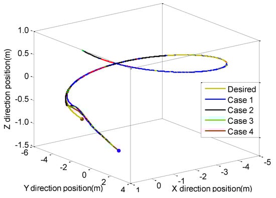
Figure 5. Trajectories (four cases).

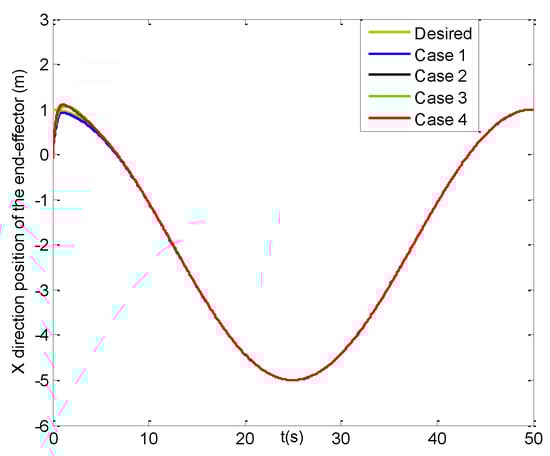
Figure 6. X direction positions of the end−effector (four cases).

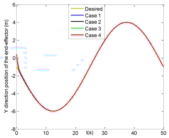
Figure 7. Y direction positions of the end−effector (four cases).

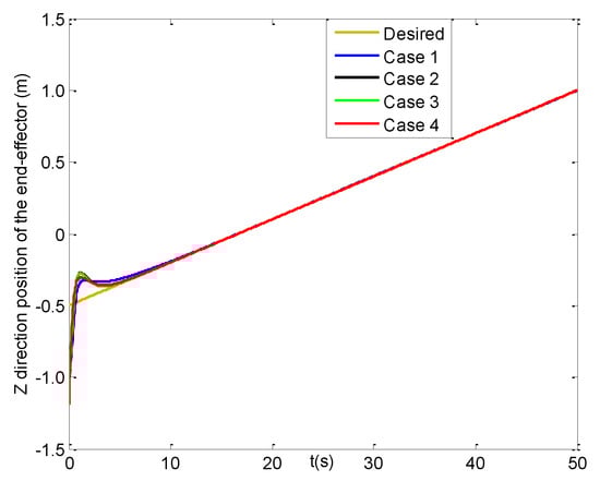
Figure 8. Z direction positions of the end−effector (four cases).

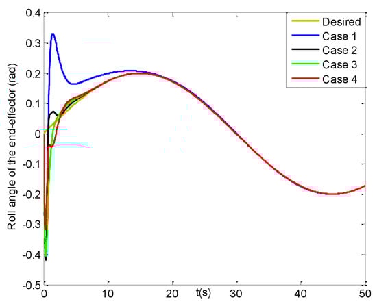
Figure 9. Roll angles of the end−effector (four cases).

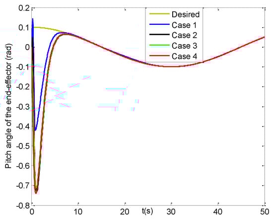
Figure 10. Pitch angles of the end−effector (four cases).

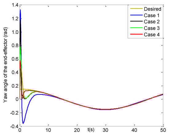
Figure 11. Yaw angles of the end−effector (four cases).

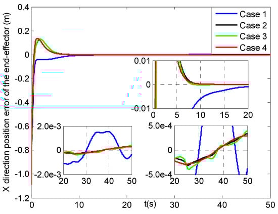
Figure 12. X direction position errors of the end−effector (four cases).

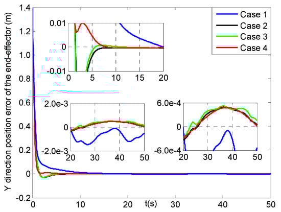
Figure 13. Y direction position errors of the end−effector (four cases).

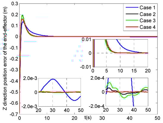
Figure 14. Z direction position errors of the end−effector (four cases).

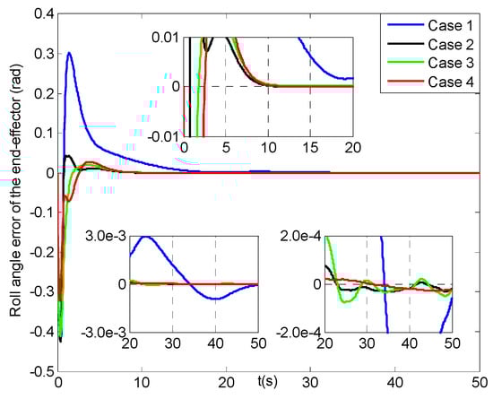
Figure 15. Roll angle errors of the end−effector (4 cases).

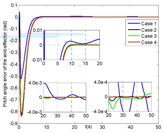
Figure 16. Pitch angle errors of the end−effector (four cases).

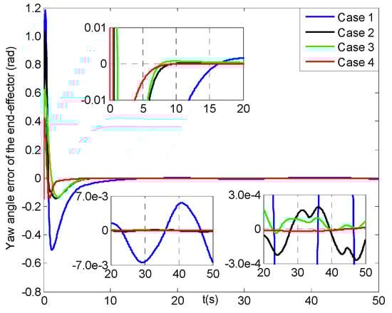
Figure 17. Yaw angle errors of the end−effector (four cases).

From Figure 12, the position errors of the end-effector in X direction for cases 2–4 can reach [−0.01, 0.01] m at about 6 s, but after three seconds the result in case 1 starts to converge more slowly. Then, Figure 13 shows that the Y direction position error of the end-effector in case 4 can arrive at [−0.01, 0.01] m within 1.5 s, and the slower is at 4 s in cases 2–3, and the slowest in case 1 till about 11 s. Figure 14 presents the position error of the end-effector in Z direction for cases 1–4, where those in cases 2–4 can reach [−0.01, 0.01] m at about 5 s and converge four seconds faster than that in case 1. Moreover, the three steady-state position errors of the end-effector in four cases can all obtain the range of [−0.002, 0.002] m, and the error values of case 4 change a little smoother than those in cases 2–3, and the roughest ones are in case 1.

Figure 15, Figure 16 and Figure 17 lay out the roll angle, pitch angle and yaw angle errors of the end-effector under four cases, respectively. Noted that the roll angle errors in cases 2–4 can attain [−0.01, 0.01] rad at about 6 s, while that in case 1 can reach till about 14 s. Though the pitch angle errors in case 1 can reach [−0.01, 0.01] rad with one second faster than those in cases 2–4, after then the latter values can realize faster convergence than that in case 1. Seen from Figure 17, the yaw angle error in case 4 can get to [−0.01, 0.01] rad at less than 4 s, and has two seconds faster than those in cases 2–3, while the one in case 1 can reach the feasible range till about 12 s. Then the yaw angle error in case 1 tends to a slower convergence rate than those in other cases. Finally, all the three steady-state orientation angle errors of the end-effector can realize the range of [−0.007, 0.007] rad, where those in case 4 have much smoother changes than those in cases 1–3, and meanwhile those in case 1 range most largely. In addition, their average position and orientation angle errors of the end-effector are listed in Table 5. It is evident that from 10 s to 50 s all of the average values for cases 2–4 are much smaller than those in case 1, especially, the last four average errors in case 4 are the smallest compared to other cases.

Table 5. Average position and orientation errors of the end-effector under four cases from 10 s to 50 s.

Case/10−3	Case 1	Case 2	Case 3	Case 4
$E_x$ (m)	1.80	0.18	0.21	0.20
$E_y$ (m)	2.90	0.37	0.34	0.35
$E_z$ (m)	1.50	0.024	0.056	0.007
$E_{\varphi }$ (rad)	5.80	0.036	0.115	0.041
$E_{\theta }$ (rad)	1.60	0.052	0.169	0.046
$E_{\psi }$ (rad)	4.90	0.143	0.207	0.016

Figure 18, Figure 19, Figure 20 and Figure 21 describe the tracking history for the three direction positions and yaw angle of the vehicle under four cases, in which all the actual values can reach the reference trajectories within about 10 s. Then, some results for the X, Y, Z direction position and yaw angle errors of the vehicle are given in Figure 22, Figure 23, Figure 24 and Figure 25. In Figure 22, the X direction position error of the vehicle in case 4 can reach [−0.01, 0.01] m at about 1.5 s, which has two seconds faster than those in cases 2–3, while that in case 1 can achieve the range till about 10 s and then converge more slowly than the former three cases. Figure 23 and Figure 24 present the Y and Z direction position errors of the vehicle in cases 1–4, respectively. And, the two position errors in case 4 can all can arrive at [−0.01, 0.01] m within 1.5 s, and those in cases 2–3 can reach more slowly between 4 s and 5 s, and the slowest those in case 1 are till about 11 s. After that, all the three position errors of the vehicle in cases 2–4 have much faster convergent rates than those in case 1. From Figure 25, the yaw angle error of the vehicle in case 4 can get to [−0.01, 0.01] rad at about 1.5 s, and after less two seconds those in cases 2–3 can achieve, while that in case 1 can attain till about 8.5 s and then converge in a slower rate. Finally, the three direction position and yaw angle errors under four cases can achieve the steady-state ranges of [–0.003, 0.003] m and [–0.004, 0.004] rad, respectively. Moreover, all of the steady-state error values in case 4 have much smoother changes than those in other cases, and the roughest in case 1.

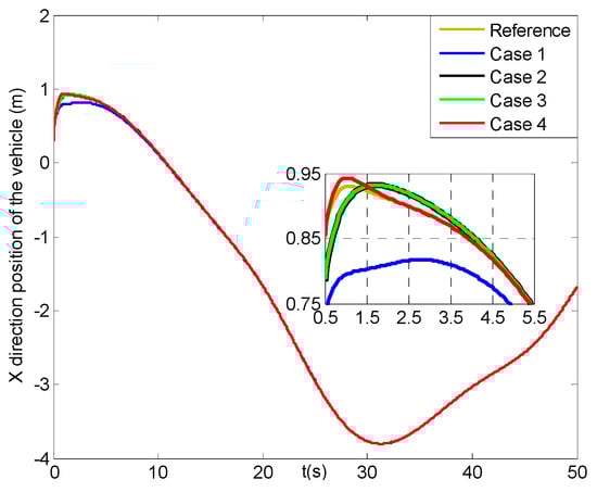
Figure 18. X direction positions of the vehicle (four cases).

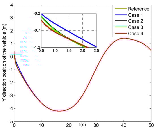
Figure 19. Y direction positions of the vehicle (four cases).

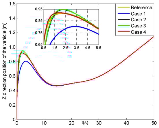
Figure 20. Z direction positions of the vehicle (four cases).

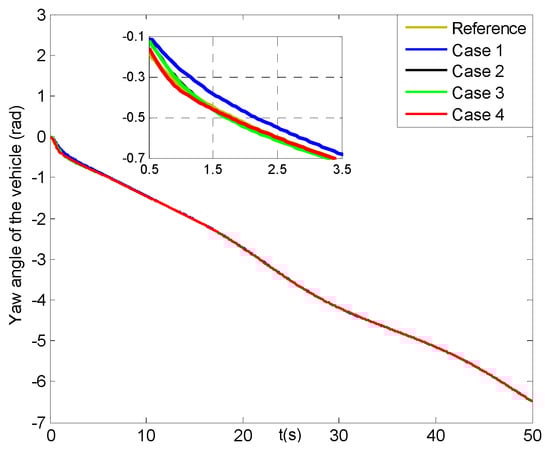
Figure 21. Yaw angles of the vehicle (four cases).

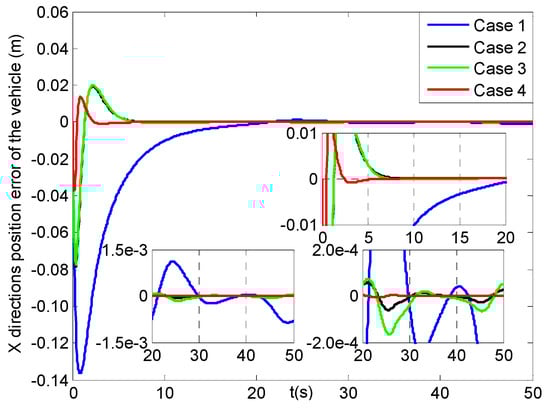
Figure 22. X direction position errors of the vehicle (four cases).

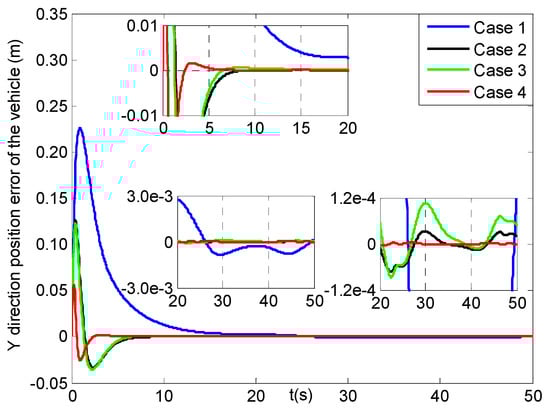
Figure 23. Y direction position errors of the vehicle (four cases).

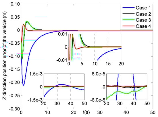
Figure 24. Z direction position errors of the vehicle (four cases).

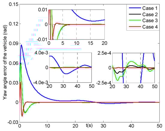
Figure 25. Yaw angle errors of the vehicle (four cases).

Besides, there are some velocity results for the three positions and yaw angle of the vehicle under four cases in Figures S1–S8, shown in the Supplementary Materials. From Figures S1–S4, the three direction velocities and yaw angle velocities of the vehicle in cases 1–4 can reach the reference values at about 5 s. In Figures S5–S7, the corresponding velocity errors in cases 1–4 can all get to [−0.01, 0.01] m/s within 7 s, while those in case 1 converge slower than other cases. In the final phase, their steady-state velocity errors in cases 2–4 can achieve the range of $[-{10}^{-4}, {10}^{-4}]$ m/s and those in case 1 are $[-7\times {10}^{-4}, 7\times {10}^{-4}]$ m/s. Then, in Figure S8 the yaw angle velocity errors of the vehicle for cases 1–4 can reach [−0.01, 0.01] rad/s within 4 s, and their steady-state errors can all arrive at $[-8\times {10}^{-4}, 8\times {10}^{-4}]$ rad/s. In the Supplementary Materials, Figures S9–S14 and S21–S26 describe the six joint position and velocity trajectories of the manipulator for tracking the reference values in four cases, respectively. Seen from them, the actual joint position and velocity trajectories can all reach the reference ones within 15 s, and their corresponding tracking error results are shown in Figures S15–S20 and S27–S32 of the Supplementary Materials. Among, it can be obtained from Figures S15–S20 that all of the six joint position errors can arrive at the range of [−0.01, 0.01] rad at about 13 s, and their steady-state errors in cases 2–4 can arrive at $[-4\times {10}^{-4}, 4\times {10}^{-4}]$ rad and those in case 1 are [–0.008, 0.008] rad. In Figures S27–S32 all of the six joint velocity errors for cases 1–4 can get to [−0.01, 0.01] rad/s within 9 s, and their steady-state errors in cases 1–4 can all achieve the range of [–0.003, 0.003] rad/s. Especially, all of the results in case 4 show the smoothest changes than those in other cases, and the roughest are in case 1.

Figure 26, Figure 27, Figure 28 and Figure 29 describe the X, Y, Z direction forces and yaw angle moments of the vehicle in four cases, respectively. Seen that in the beginning all of the forces and moments change largely, and after five seconds they turn to smooth trends. In addition, the related six joint moments of the manipulator are shown in Figures S33–S38 of the Supplementary Materials. Then, the average force and moment values of the UVMS is listed in Table 6, where the average force and moment values have less 0.1 N and 0.4 N m differences among the four cases, respectively. That means that after about 10 s, their energy consumptions for cases 1–4 approach to the same levels, which is consist with the results in Figures S33–S38. Combining the above analysis for the tracking errors of the UVMS, we can obtain that the proposed control system in case 4 can have faster convergence and higher precision tracking performance compared to other three cases.

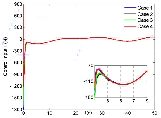
Figure 26. X direction forces for the first control input of the vehicle (four cases).

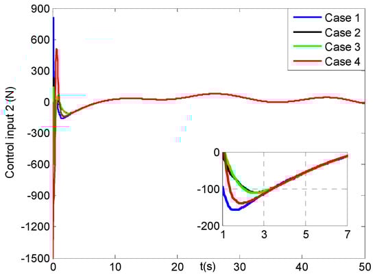
Figure 27. Y direction forces for the second control input of the vehicle (four cases).

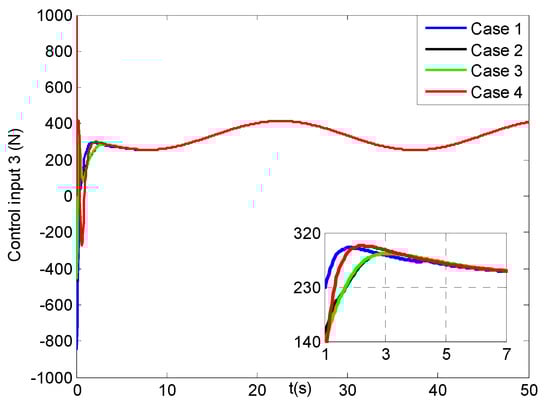
Figure 28. Z direction forces for the third control input of the vehicle (four cases).

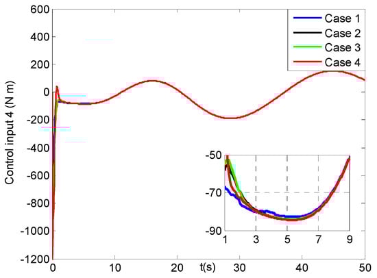
Figure 29. Yaw angle moments for the fourth control input of the vehicle (four cases).

Table 6. Average force and moment values of the UVMS under four cases from 10 s to 50 s.

Terms	Case1	Case 2	Case 3	Case 4
$E_{\tau 1}$ (N)	32.5307	32.5300	32.5211	32.5636
$E_{\tau 2}$ (N)	39.6768	39.7046	39.7017	39.7052
$E_{\tau 3}$ (N)	338.6749	338.6780	338.6748	338.6907
$E_{\tau 4}$ (N m)	112.4979	112.4290	112.4317	112.4208
$E_{\tau 5}$ (N m)	120.8286	120.5714	120.5745	120.5689
$E_{\tau 6}$ (N m)	105.9977	106.2860	106.2694	106.3245
$E_{\tau 7}$ (N m)	45.0472	45.1208	45.1160	45.1327
$E_{\tau 8}$ (N m)	5.4377	5.4329	5.4334	5.4321
$E_{\tau 9}$ (N m)	0.6668	0.6648	0.6651	0.6641
$E_{\tau 10}$ (N m)	0.5632	0.5658	0.5657	0.5656

Figure 30 and Figure 31 represent the components and their estimations of the lumped disturbance vector for the UVMS in case 4, respectively. Some related results in other three cases are shown in Figures S39–S44 of the Supplementary Materials. Despite that in the initial time there exist big differences between the lumped disturbance vectors and their estimations for cases 1–4, after several seconds the disturbance estimations in four cases can all achieve much better approximation to the lumped disturbances. The reason is that the ESO is applied to attenuate the effects of the complex lumped disturbances on the control systems. Furthermore, the average disturbance estimation errors under four cases from 10 s to 50 s are listed in Table 7. Noted that their average values are small and have few differences among four cases. Since the tracking errors in case 4 show much smoother variation compared to those in other cases, it demonstrates that the proposed control method has stronger robustness of resisting disturbances.

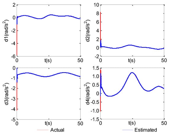
Figure 30. d1−d4 and their estimations (case 4).

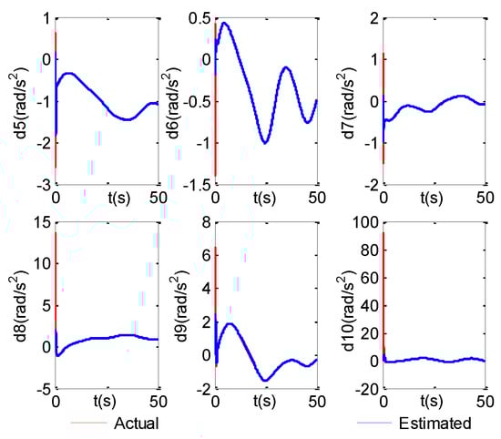
Figure 31. d5−d10 and their estimations (case 4).

Table 7. Average estimation errors of the lumped disturbances under four cases from 10 s to 50 s.

Case/10−3	Case1	Case 2	Case 3	Case 4
$E_{d1}$ (m/s2)	0.6313	0.6286	0.6280	0.6319
$E_{d2}$ (m/s2)	1.1	1.1	1.1	1.1
$E_{d3}$ (m/s2)	0.2732	0.2729	0.2730	0.2724
$E_{d4}$ (rad/s2)	1.7	1.7	1.7	1.7
$E_{d5}$ (rad/s2)	1.1	1.1	1.1	1.1
$E_{d6}$ (rad/s2)	1.7	1.7	1.7	1.7
$E_{d7}$ (rad/s2)	0.1451	0.1455	0.1459	0.1443
$E_{d8}$ (rad/s2)	1.3	1.3	1.3	1.3
$E_{d9}$ (rad/s2)	2.5	2.5	2.5	2.5
$E_{d10}$ (rad/s2)	6.2	6.3	6.3	6.2

In conclusion, the simulation comparative results validate that the proposed controller can achieve the better tracking performance and stronger robustness of disturbance rejection.

5. Conclusions

In this paper, the adaptive NFTSMC scheme integrating with ESO is proposed for the trajectory tracking of the UVMS under the lumped disturbances. First, the quaternion-based CLIKA is utilized for avoiding the integral drifts in the inverse kinematics. The proposed controller mainly contains the modified NFTSMS and ESO, and the adaptive control law. And, the applied NFTSMS can make the tracking errors achieve the fast convergence, together with avoiding the singularity. The utilization of the ESO is to estimate the lumped disturbances so that the estimation error can converge to the origin in fixed time. At the same time, appending the saturation function to the ESO instead of the signum function is to reduce the chattering effect. Besides, the continuous fractional PI-type controller with the adaptive laws is introduced in the control input, so that it can approximate the conventional discontinuous robust term to attenuate the chattering because of the discontinuity. Based on the Lyapunov theory, the control system is proved to have asymptotical stability. Comparative simulations with several other methods demonstrate that the proposed control system have better tracking performance and stronger robustness against disturbances. In the future research, we will incorporate the redundancy resolution scheme into the proposed control strategy to perform the simulation test of the UVMS, in which the redundancy resolution can realize the secondary objectives, such as avoiding manipulator joint limits and singularities, minimizing the vehicle motion, thrusters fault tolerant, etc. And, it can provide a theoretical basis for the later experiments. When the conditions of the laboratory permit, the control strategy can be applied for practicing to verify the reliability of the controller via experimental tests.

References

- Zereik, E.; Bibuli, M.; Miškovic, N.; Ridao, P.; Pascoal, A. Challenges and future trends in marine robotics. Annu. Rev. Control 2018, 46, 350–368. [Google Scholar] [CrossRef]
- Sivčev, S.; Coleman, J.; Omerdić, E.; Dooly, G.; Toal, D. Underwater manipulators: A review. Ocean Eng. 2018, 163, 431–450. [Google Scholar] [CrossRef]
- Antonelli, G.; Chiaverini, S. Fuzzy redundancy resolution and motion coordination for underwater vehicle-manipulator systems. IEEE Trans. Fuzzy Syst. 2003, 11, 109–120. [Google Scholar] [CrossRef]
- Soylu, S.; Buckham, B.J.; Podhorodeski, R.P. Redundancy resolution for underwater mobile manipulators. Ocean Eng. 2010, 37, 325–343. [Google Scholar] [CrossRef]
- Wang, Y.Y.; Jiang, S.R.; Yan, F.; Gu, L.Y.; Chen, B. A new redundancy resolution for underwater vehicle–manipulator system considering payload. Int. J. Adv. Robot. Syst. 2017, 14, 1–10. [Google Scholar] [CrossRef]
- Han, J.H.; Chung, W.K. Active use of restoring moments for motion control of an underwater vehicle-manipulator system. IEEE J. Ocean. Eng. 2014, 39, 100–109. [Google Scholar] [CrossRef]
- Thanh, H.L.; Vu, M.T.; Mung, N.X.; Nguyen, N.P.; Phuong, N.T. Perturbation observer-based robust control using a multiple sliding surfaces for nonlinear systems with influences of matched and unmatched uncertainties. Mathematics 2020, 8, 1371. [Google Scholar] [CrossRef]
- Wei, Y.H.; Zheng, Z.; Li, Q.Q.; Jiang, Z.L.; Yang, P.F. Robust tracking control of an underwater vehicle and manipulator system based on double closed-loop integral sliding mode. Int. J. Adv. Robot. Syst. 2020, 17, 1729881420941778. [Google Scholar] [CrossRef]
- Vu, M.T.; Le, T.-H.; Thanh, H.L.; Huynh, T.-T.; Van, M.; Hoang, Q.-D.; Do, T.D. Robust position control of an over-actuated underwater vehicle under model uncertainties and ocean current effects using dynamic sliding mode surface and optimal allocation control. Sensors 2021, 21, 747. [Google Scholar] [CrossRef]
- Vu, M.T.; Thanh, H.L.; Huynh, T.-T.; Do, Q.T.; Do, T.D.; Hoang, Q.-D.; Le, T.-H. Station-keeping control of a hovering over-actuated autonomous underwater vehicle under ocean current effects and model uncertainties in horizontal plane. Access 2021, 9, 6855–6867. [Google Scholar] [CrossRef]
- Qiao, L.; Zhang, W.D. Trajectory tracking control of AUVs via adaptive fast nonsingular integral terminal sliding mode control. IEEE Trans. Ind. Informat. 2020, 16, 1248–1258. [Google Scholar] [CrossRef]
- Kumar, N.; Rani, M. An efficient hybrid approach for trajectory tracking control of autonomous underwater vehicles. Appl. Ocean Res. 2020, 95, 1–10. [Google Scholar] [CrossRef]
- Zhong, Y.G.; Yang, F. Dynamic modeling and adaptive fuzzy sliding mode control for multi-link underwater manipulators. Ocean Eng. 2019, 187, 106202. [Google Scholar] [CrossRef]
- Xiong, S.F.; Wang, W.H.; Liu, X.D.; Chen, Z.Q.; Wang, S. A novel extended state observer. ISA Trans. 2015, 58, 309–317. [Google Scholar] [CrossRef]
- Levant, A. Principles of 2-sliding mode design. Automatica 2007, 43, 576–586. [Google Scholar] [CrossRef]
- Mohan, S.; Kim, J. Coordinated motion control in task space of an autonomous underwater vehicle–manipulator system. Ocean Eng. 2015, 104, 155–167. [Google Scholar] [CrossRef]
- Londhe, P.S.; Mohan, S.; Patre, B.M.; Waghmare, L.M. Robust task-space control of an autonomous underwater vehicle-manipulator system by PID-like fuzzy control scheme with disturbance estimator. Ocean Eng. 2017, 139, 1–13. [Google Scholar] [CrossRef]
- Cui, R.X.; Chen, L.P.; Yang, C.G.; Chen, M. Extended state observer-based integral sliding mode control for an underwater robot with unknown disturbances and uncertain nonlinearities. IEEE Trans. Ind. Electron. 2017, 64, 6785–6795. [Google Scholar] [CrossRef]
- Wang, H.D.; Lin, Z.; Karkoub, M.; Kerimoglu, D. Extended state observer based sliding mode control with prescribed performance for underwater vehicle manipulator system. In Proceedings of the 5th International Conference on Automation, Control and Robotics Engineering, Dalian, China, 19–20 September 2020; pp. 368–372. [Google Scholar]
- Patre, B.M.; Londhe, P.S.; Waghmare, L.M.; Mohan, S. Disturbance estimator based non-singular fast fuzzy terminal sliding mode control of an autonomous underwater vehicle. Ocean Eng. 2018, 159, 372–387. [Google Scholar] [CrossRef]
- Guerrero, J.; Torres, J.; Creuze, V.; Chemori, A. Adaptive disturbance observer for trajectory tracking control of underwater vehicles. Ocean Eng. 2020, 200, 107080. [Google Scholar] [CrossRef]
- Basin, M.; Panathula, C.B.; Shtessel, Y. Multivariable continuous fixed-time second-order sliding mode control: Design and convergence time estimation. IET Control Theory Appl. 2017, 11, 1104–1111. [Google Scholar] [CrossRef]
- Chiaverini, S.; Siciliano, B. The unit quaternion: A useful tool for inverse kinematics of robot manipulators. SAMS 1999, 35, 45–60. [Google Scholar]
- Podder, T.K. Motion Planning of Autonomous Underwater Vehicle-Manipulator Systems. Ph.D. Thesis, University of Hawai’i, Manoa, HI, USA, 2000. [Google Scholar]
- Fossen, T.I. Guidance and Control of Ocean Vehicles; John Wiley & Sons Inc.: Chichester, UK, 1994; p. 85. [Google Scholar]
- Bhat, S.P.; Bernstein, D.S. Geometric homogeneity with applications to finite-time stability. Math. Control Signals Syst. 2005, 17, 101–127. [Google Scholar] [CrossRef]
- Tao, G. A simple alternative to the Barbalat lemma. IEEE Trans. Autom. Control 1997, 42, 698. [Google Scholar] [CrossRef]
- Yang, L.; Yang, J.Y. Nonsingular fast terminal sliding-mode control for nonlinear dynamical systems. Int. J. Robust. Nonlinear Control 2011, 21, 1865–1879. [Google Scholar] [CrossRef]
- Shahnazi, R.; Shanechi, H.; Pariz, N. Position control of induction and DC servomotors: A novel adaptive fuzzy PI sliding mode control. IEEE Trans. Energy Convers. 2008, 23, 138–147. [Google Scholar] [CrossRef]
- Vu, M.T.; Van, M.; Bui, D.H.P.; Do, Q.T.; Huynh, T.-T.; Lee, S.D.; Choi, H.-S. Study on dynamic behavior of unmanned surface vehicle-linked unmanned underwater vehicle system for underwater exploration. Sensors 2020, 20, 1329. [Google Scholar] [CrossRef]
- Wei, Y.H.; Zhou, W.X.; Jia, X.Q.; Wang, Z.P. Model decoupling and multi-controller joint control of horizontal movement for AUV. J. Huazhong Univ. Sci. Tech. 2016, 44, 37–42. [Google Scholar] [CrossRef]
- Wei, Y.H. The Control Technology of the UVMS; Harbin Engineering University Press: Harbin, China, 2017; p. 60. [Google Scholar]
- Wang, Y.Y. Research on Coordinated Control of Autonomous Underwater Vehicle-Manipulator Systems. Ph.D. Thesis, Zhejiang University, Hangzhou, China, 2016. [Google Scholar]
- Huang, S.S.; Fan, J. The proving and application of a new set of equations for kinematic analysis of robots. Robot 1994, 16, 257–263. [Google Scholar]
- Shoults, G.A. Dynamics Control of an Underwater Robotic Vehicle with an n-Axis Manipulator. Ph.D. Thesis, Washington University, St. Louis, MO, USA, 1996. [Google Scholar]
Publisher’s Note: MDPI stays neutral with regard to jurisdictional claims in published maps and institutional affiliations. |
© 2021 by the authors. Licensee MDPI, Basel, Switzerland. This article is an open access article distributed under the terms and conditions of the Creative Commons Attribution (CC BY) license (https://creativecommons.org/licenses/by/4.0/).