
Meteorological Navigation by Integrating Metocean Forecast Data and Ship Performance Models into an ECDIS-like e-Navigation Prototype Interface


Abstract
1. Introduction
- The key element, and first requirement for the work, is the definition of a framework for an effective integration of detailed metocean data and ship modeling approaches with a graphical user interface very close to the industry standard utilized by seafarers in their real life at sea.
- From the development point of view, the main requirement is that such an integration be realized through a modular structure allowing a short response time for the “on-line” use, and allowing also systematic tuning and validation of algorithms and datasets.
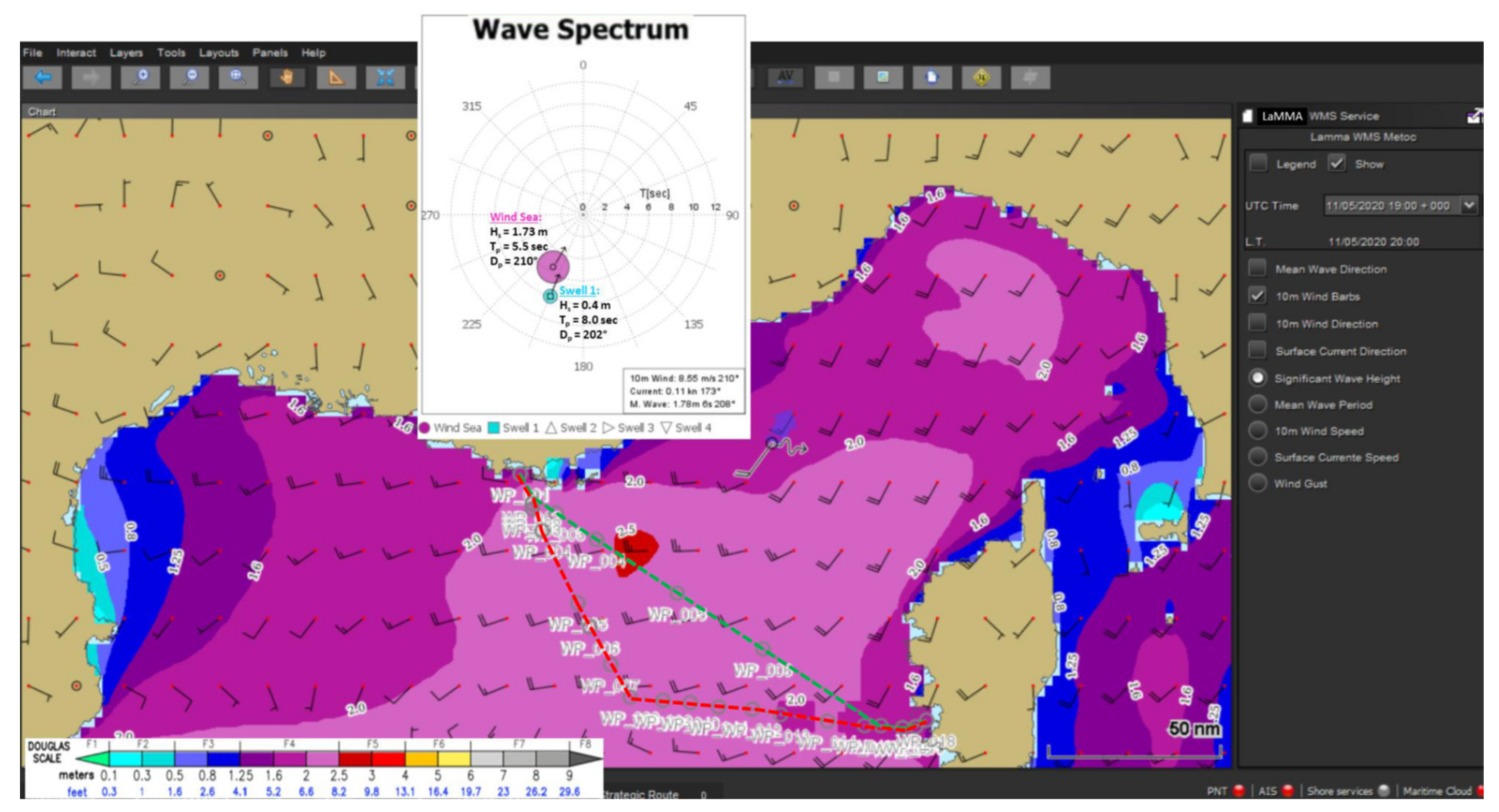
2. The Prototype Navigation Interface: An Overview
3. Data and Models
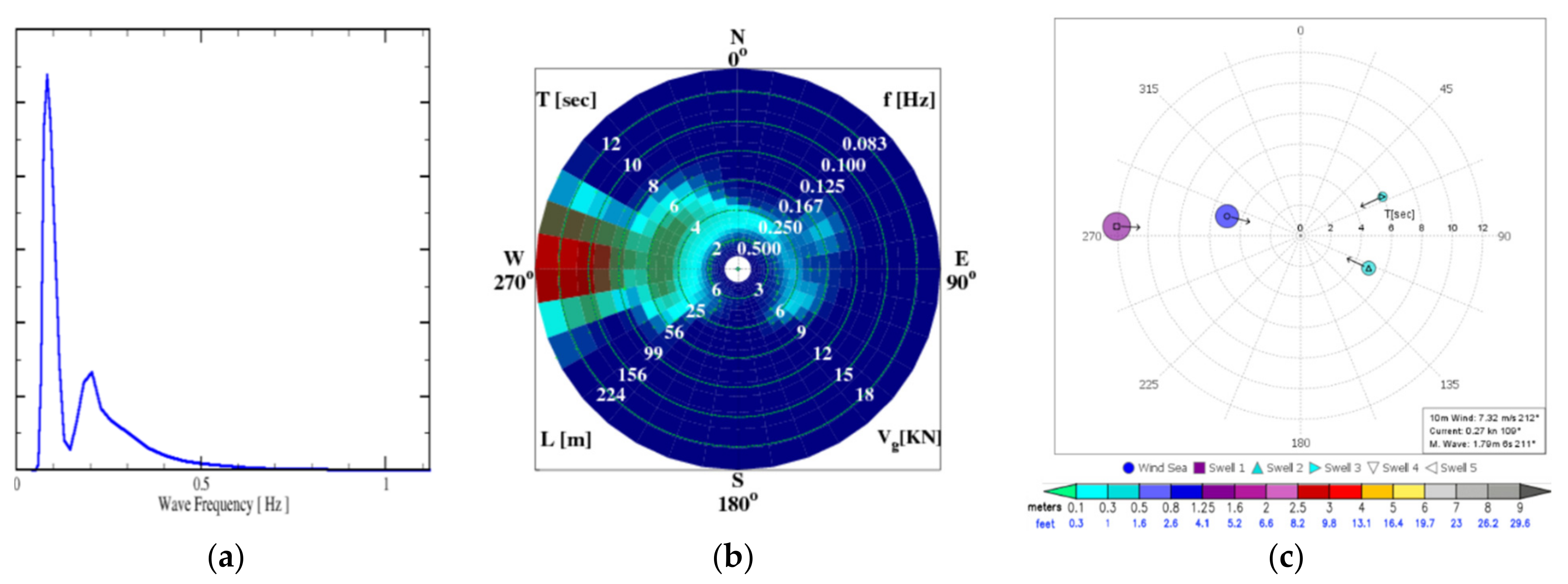
3.1. Metocean Data
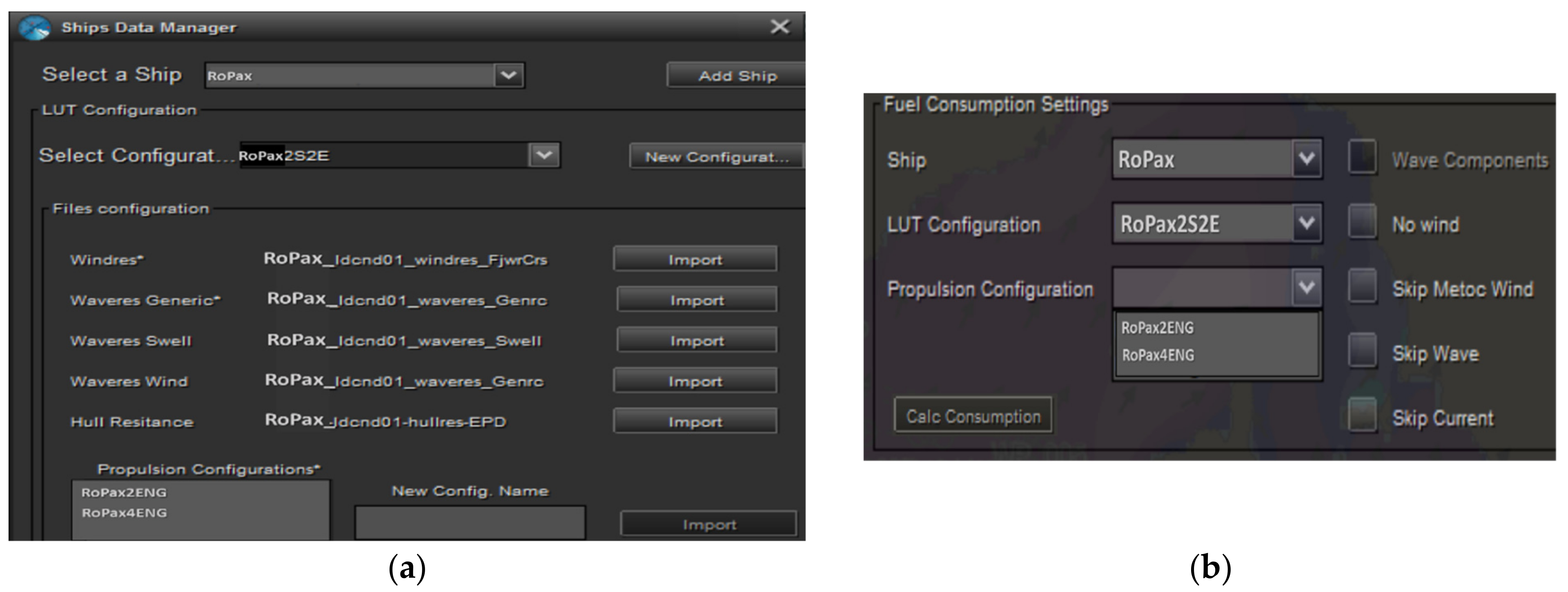
3.2. Ship Modeling
4. Discussion of Illustrative Case Studies
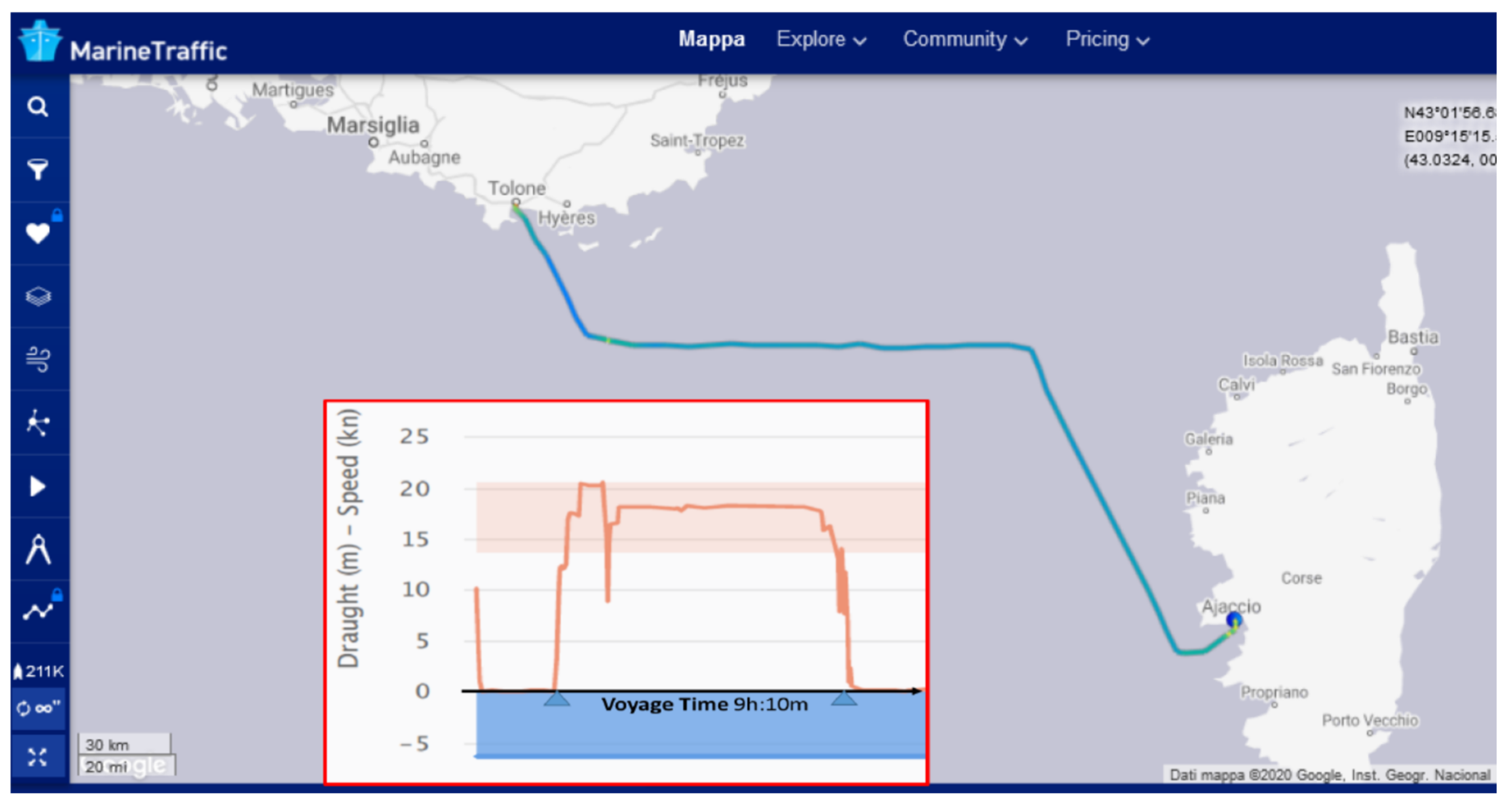
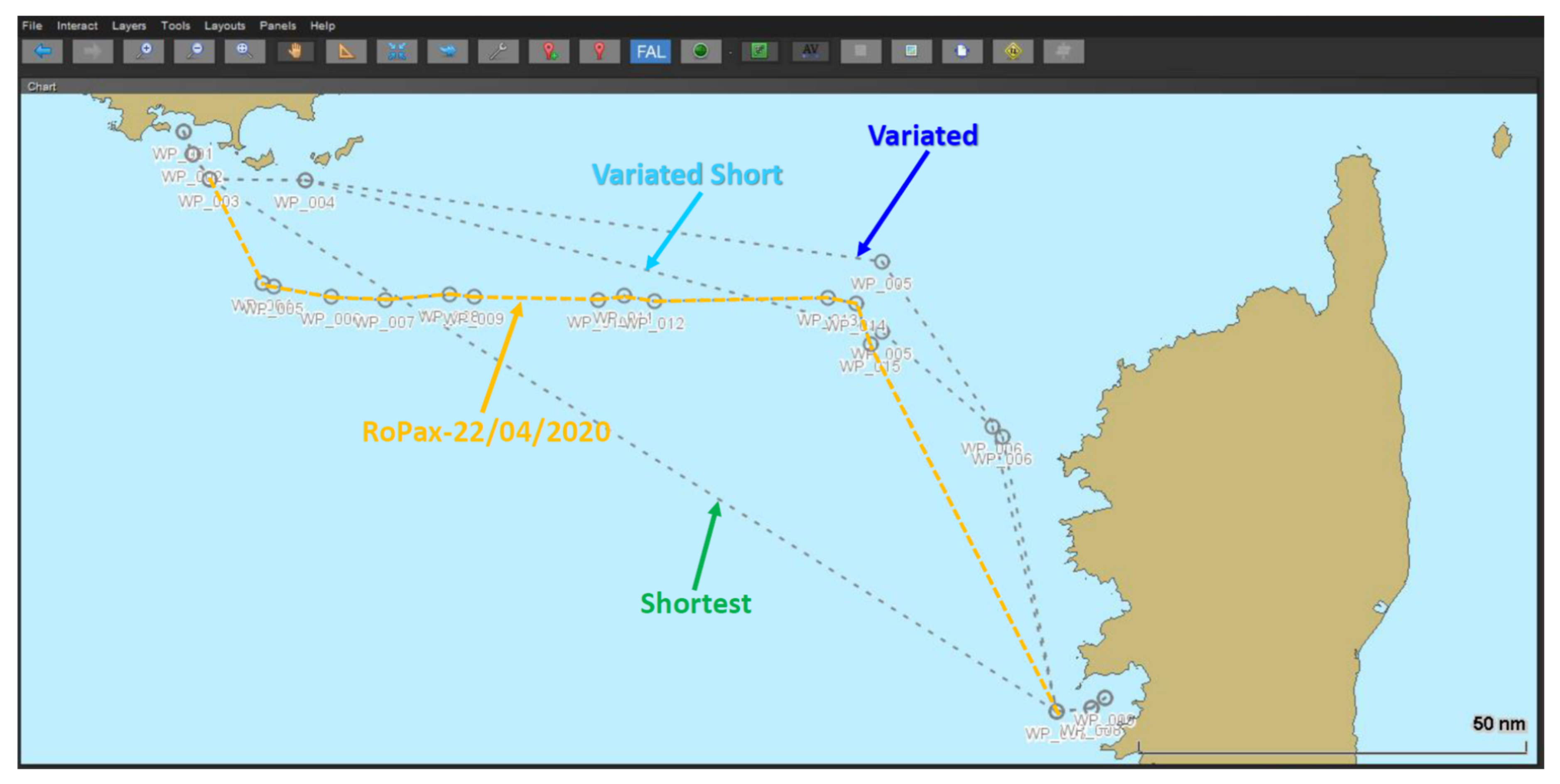
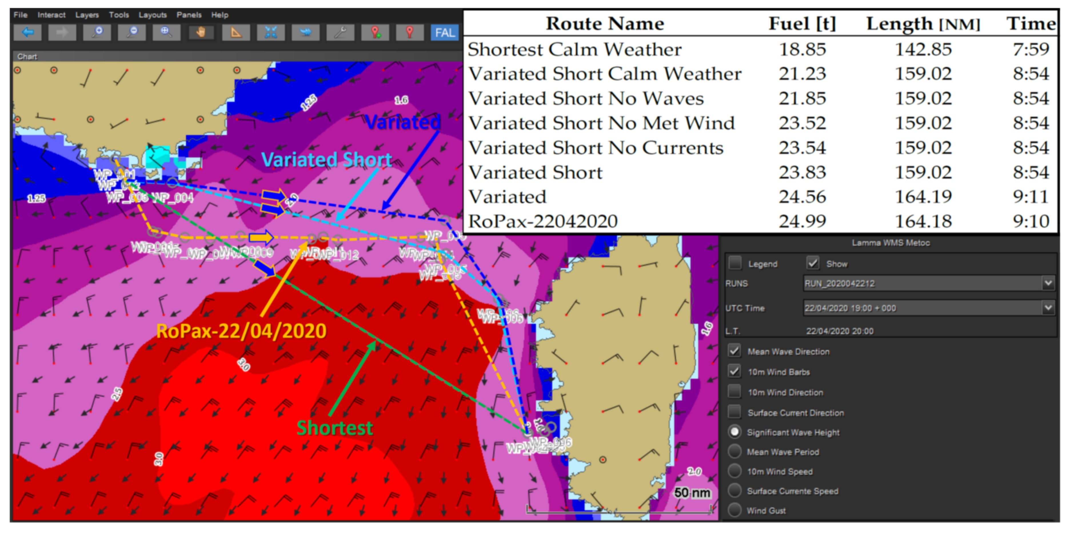
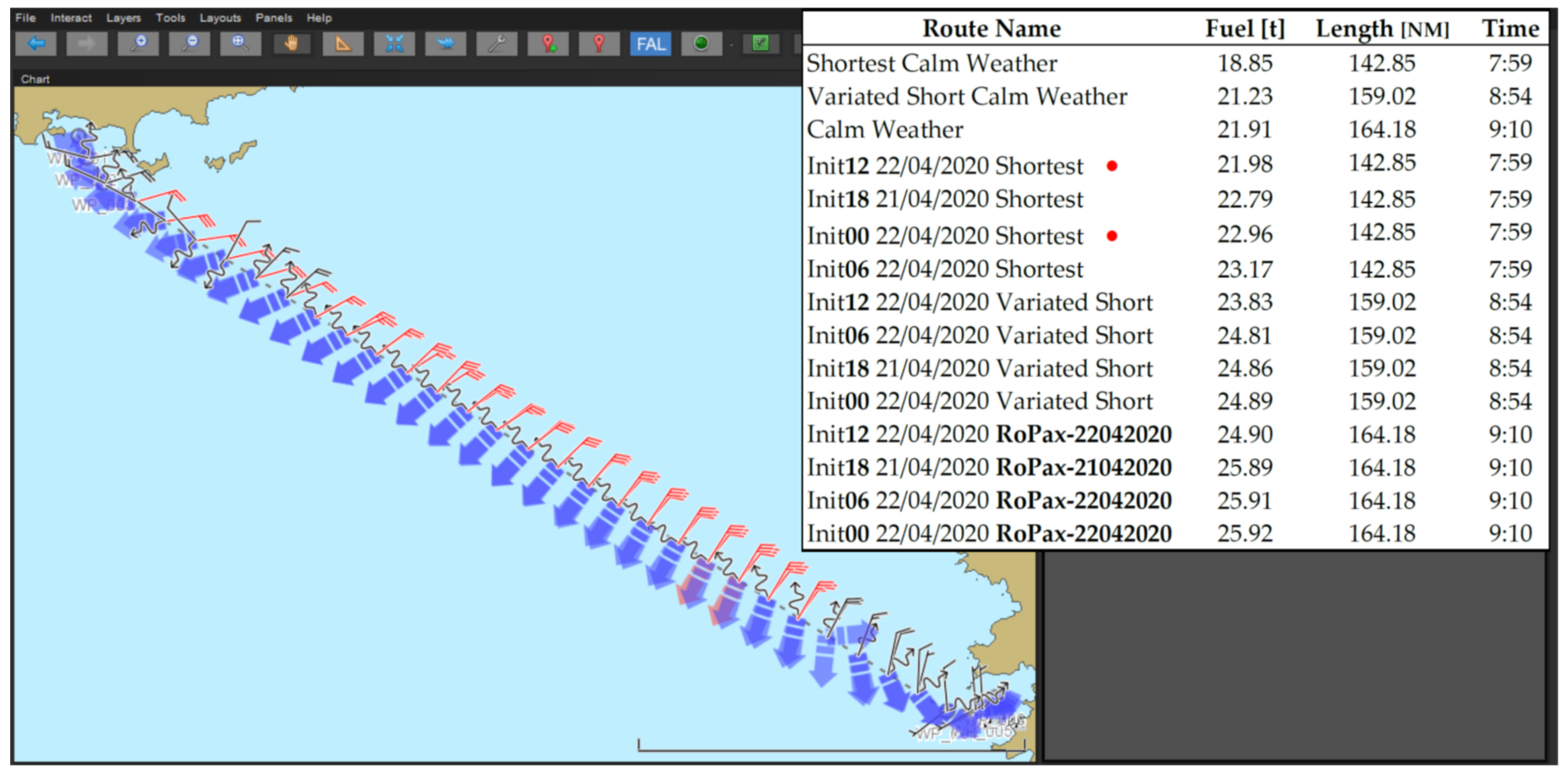
4.1. RoPax on a Short Route in Perturbed Metocean Conditions. Center-North Mediterranean Sea (Sea of Corse)
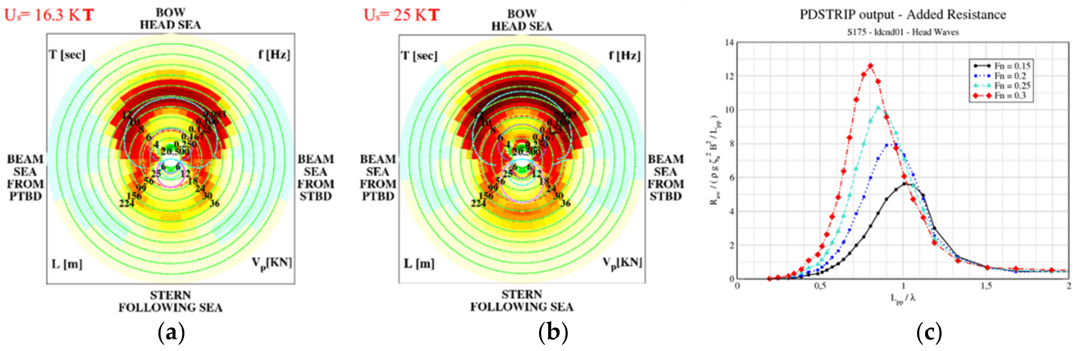
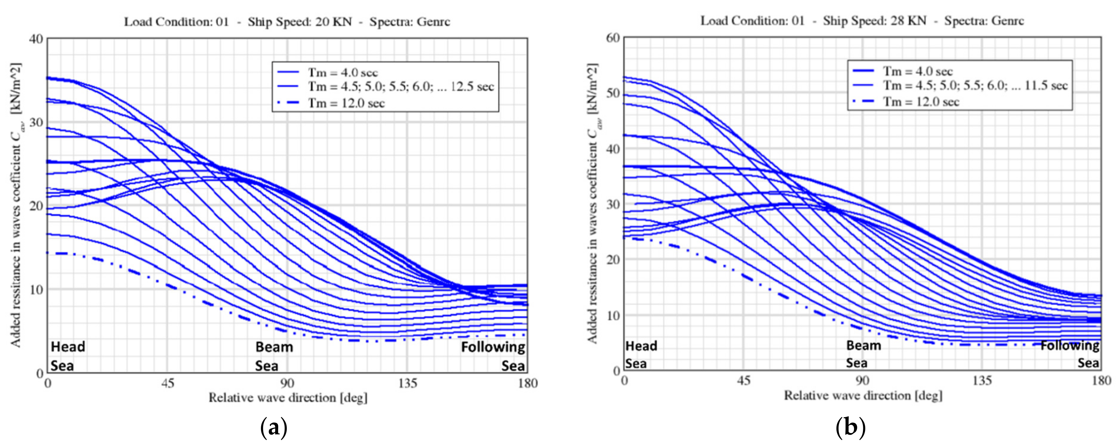
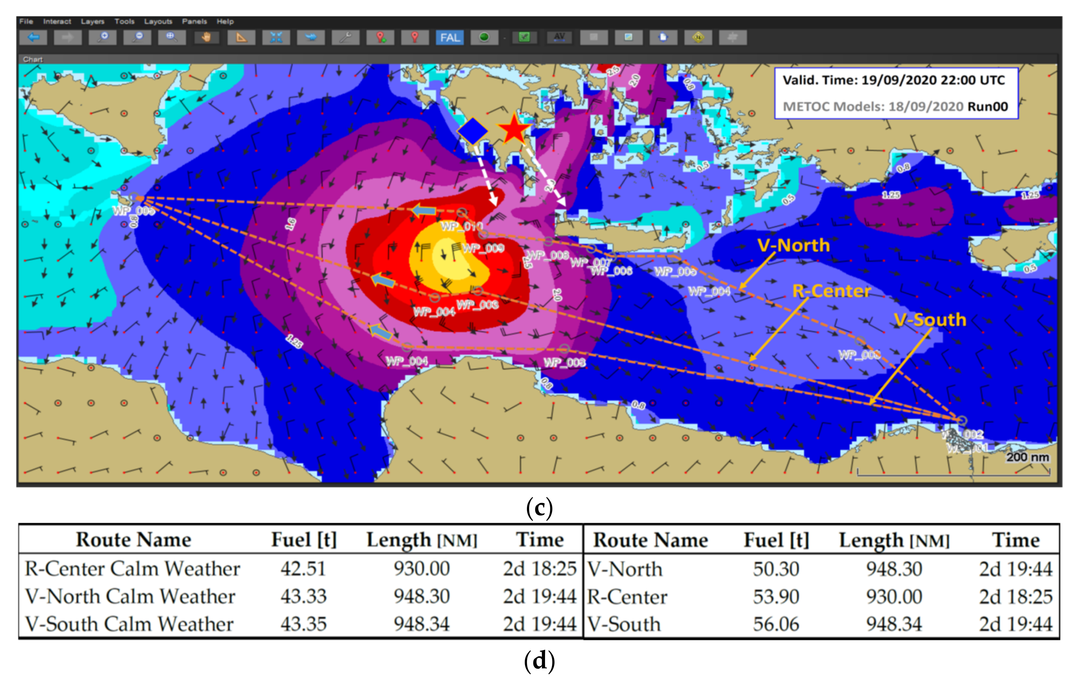
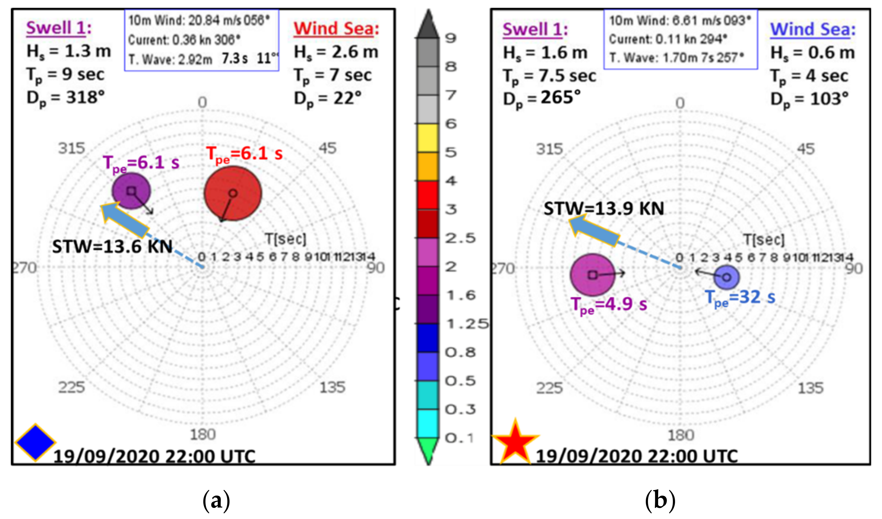
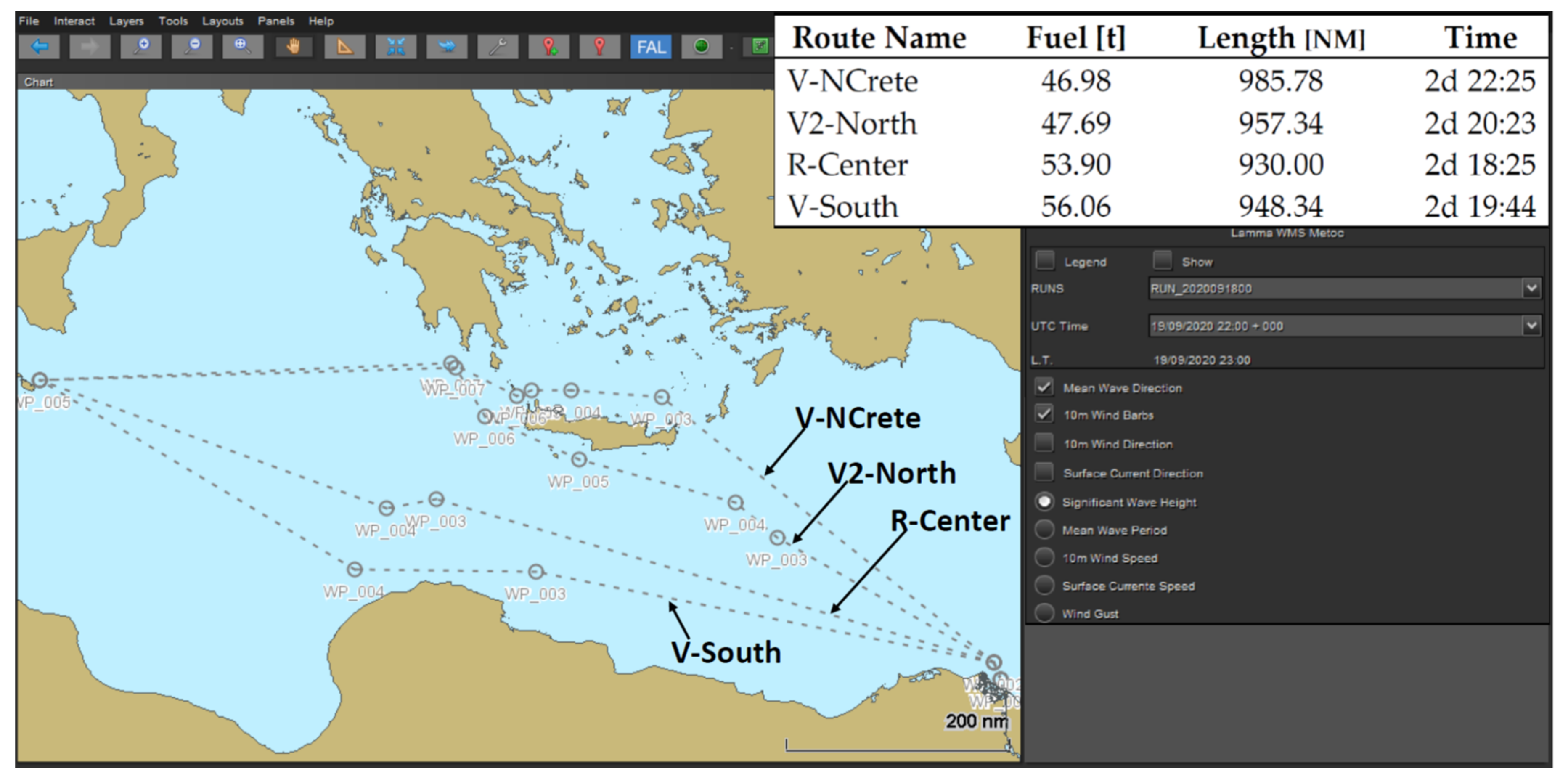
4.2. S175 Containership on a Medium Length Route in Heavy Weather. Eastern Mediterranean Sea
5. Conclusions
Author Contributions
Funding
Institutional Review Board Statement
Informed Consent Statement
Data Availability Statement
Conflicts of Interest
References
- Stopford, M. Maritime Economics, 3rd ed.; Routledge: London, UK, 2008. [Google Scholar]
- Christiansen, M.; Fagerholt, K.; Nygreen, B.; Ronen, D. Maritime Transportation. In Handbooks in Operations Research and Management Science; Barnhart, C., Laporte, G., Eds.; Elsevier: Amsterdam, The Netherlands, 2007; Volume 14, pp. 189–284. [Google Scholar]
- Windek, V. A Liner Shipping Network Design. Routing and Scheduling Considering Environmental Influences. Ph.D. Thesis, Hamburgh University, Hamburgh, Germany, 2013. [Google Scholar]
- Weintrit, A. Marine Navigation and Safety of Sea Transportation; Taylor & Francis Group: London, UK, 2009. [Google Scholar]
- Bouman, E.A.; Lindstad, E.; Rialland, A.I.; Strømman, A.H. State-of-the-art technologies, measures, and potential for reducing GHG emissions from shipping. A review. Transp. Res. Part D 2017, 52, 408–442. [Google Scholar] [CrossRef]
- Smith, T.W.P.; O’Keeffe, E.; Aldous, L.; Agnolucci, P. Assessment of Shipping’s Efficiency Using Satellite AIS Data; UCL Energy Institute: London, UK, 2013. [Google Scholar]
- DNV-GL. Maritime Forecast to 2050; Energy Transition Outlook: Hovik, Norway, 2020. [Google Scholar]
- Trancossi, M. What price of speed? A critical revision through constructal optimization of transport modes. Int. J. Energy Environ. Eng. 2016, 7, 425–448. [Google Scholar] [CrossRef]
- Psaraftis, H.N. Speed Optimization vs. Speed Reduction: The Choice between Speed Limits and a Bunker Levy. Sustainability 2019, 11, 2249. [Google Scholar] [CrossRef]
- Meyer, J.; Stahlbock, R.; Voß, S.; Voss, S. Slow Steaming in Container Shipping. In Proceedings of the 2012 45th Hawaii International Conference on System Sciences, Maui, HI, USA, 4–7 January 2012; pp. 1306–1314. [Google Scholar]
- IMO. Just in Time Arrival Guide: Barriers and Potential Solutions; IMO GloMEEP Project Coordination Unit: London, UK, 2020. [Google Scholar]
- Panagakos, G.; Pessôa, T.D.S.; Dessypris, N.; Barfod, M.B.; Psaraftis, H.N. Monitoring the Carbon Footprint of Dry Bulk Shipping in the EU: An Early Assessment of the MRV Regulation. Sustainability 2019, 11, 5133. [Google Scholar] [CrossRef]
- Allal, A.A.; Mansouri, K.; Youssfi, M.; Qbadou, M. Ship Operational Measures Implementation’s Impact on Energy-Saving and GHG Emission. In Proceedings of the Advanced Intelligent Systems for Sustainable Development (AI2SD’2019): Advanced Intelligent Systems Applied to Energy, Marrakech, Morocco, 8–11 July 2019; Volume 2, pp. 307–319. [Google Scholar]
- Canbulat, O.; Aymelek, M.; Turan, O.; Boulougouris, E. A Bayesian Belief Network Model for Integrated Energy Efficiency of Shipping. In Maritime Women: Global Leadership; Springer: Cham, Switzerland, 2018; pp. 257–273. [Google Scholar]
- Campana, E.F.; Ciappi, E.; Bertram, V. New IT Technologies for a Sustainable Blue Growth. In Proceedings of the 12th Symposium on High-Performance Marine Vehicles, Cortona, Italy, 12–14 October 2020. [Google Scholar]
- Matsuo, K.; Tanigawa, F. On Future Strategy and Technology Roadmap of Maritime Industry. In Proceedings of the 12th Symposium on High-Performance Marine Vehicles, Cortona, Italy, 12–14 October 2020. [Google Scholar]
- Procee, S. Considerations for a Novel Augmented Reality Display on the Ship’s Bridge. In Proceedings of the 12th Symposium on High-Performance Marine Vehicles, Cortona, Italy, 12–14 October 2020. [Google Scholar]
- IMO e-Navigation. Available online: www.imo.org/en/OurWork/Safety/Navigation/Pages/eNavigation.aspx (accessed on 22 September 2020).
- Patraiko, E.D. Introducing the e-Navigation Revolution. Seaways. Int. J. Naut. Inst. Lond. 2007. [Google Scholar]
- Weintrit, A. Development of the IMO e-Navigation Concept. Common Maritime Data Structure. In Modern Transport Telematics; Mikulski, J., Ed.; Springer: Berlin/Heidelberg, Germany, 2011; Volume 239. [Google Scholar]
- IALA e-Navigation Portal. Available online: www.iala-aism.org/technical/e-navigation/ (accessed on 22 September 2020).
- Lind, M.; Bergmann, M.; Hägg, M.; Karlsson, F.; Siwe, U.; Watson, R. Sea Traffic Management—The Route to the Future. In Proceedings of the 17th Conference on Computer and IT Applications in the Maritime Industries (COMPIT), Pavone, Italy, 14–16 May 2018. [Google Scholar]
- STM Project. Available online: www.seatrafficmanagement.info (accessed on 22 September 2020).
- Koga, S. Major Challenges and Solutions for Utilizing Big Data in the Maritime Industry. Master’s Thesis, World Maritime University, Malmö, Sweden, 2015. [Google Scholar]
- Simonsen, M.H.; Larsson, E.; Mao, W.; Ringsberg, W. State-of-the-art within ship weather routing. In Proceedings of the ASME 2015, 34th International Conference on Ocean, Offshore and Arctic Engineering, St. John’s, NL, Canada, 31 May–5 June 2015. [Google Scholar]
- Walther, L.; Rizvanolli, A.; Wendebourg, M.; Jahn, C. Modeling and Optimization Algorithms in Ship Weather Routing. Int. J. e-Navig. Marit. Econ. 2016, 4, 31–45. [Google Scholar] [CrossRef]
- Wiśniewski, B.; Szymański, M. Comparison of ship performance optimization systems and the bon voyage onboard routing system. Sci. J. Zesz. Nauk. Marit. Univ. Szczec. 2016, 47, 106–115. [Google Scholar]
- Perera, L.P.; Guedes Soares, C. Weather routing and safe ship handling in the future of shipping. Ocean Eng. 2017, 130, 684–695. [Google Scholar] [CrossRef]
- Lópeza, J.M.L.; Calabriaa, L.; Tannera, M.; Martíneza, J.; Giméneza, J.A. Vessl as a tool for macro-analyses at European level. STM Validation Project results calculated by the use of Short Sea Shipping data mining. In Proceedings of the 8th Transport Research Arena TRA 2020, Helsinki, Finland, 27–30 April 2020. [Google Scholar]
- Takashima, K.; Mezaoui, B.; Shoji, R. On the fuel saving operation for coastal merchant ships using weather routing. Int. J. Mar. Nav. Saf. Sea Transp. 2009. [Google Scholar]
- Michaelides, M.P.; Herodotou, H.; Lind, M.; Watson, R.T. Port-2-Port communication enhancing Short Sea Shipping performance: The case study of Cyprus and the Eastern Mediterranean. Sustainability 2019, 11, 1912. [Google Scholar] [CrossRef]
- Martìnez de Osès, F.X.; Castells, M. Wave height incidence on Mediterranean Short Sea Shipping routes. Tethys 2006, 3, 3–8. [Google Scholar]
- Wärtsilä Smart Voyage Optimisation. Available online: www.wartsila.com/smart-voyage (accessed on 10 October 2020).
- NAVTOR Weather Routeing. Available online: www.navtor.com/weatherservices.html (accessed on 10 October 2020).
- JRC Japan. J-Marine Cloud. Weather Routing and Smart Ship Service. Available online: www.jmarinecloud.com/eng/corporation/routing_pro (accessed on 16 November 2020).
- Papanikolaou, A. Holistic ship design optimization: Merchant and naval ships. Ship Sci. Technol. 2011, 5, 9. [Google Scholar] [CrossRef][Green Version]
- Papanikolaou, A.; Flikkema, M.; Harries, S.; Marzi, J.; Le Néna, R.; Torben, S.; Yrjänäinen, A. Tools and Applications for the Holistic Ship Design. In Proceedings of the 8th Transport Research Arena, Helsinki, Finland, 27–30 April 2020. [Google Scholar]
- Guangrong, Z. Intelligent Design and Operation of Ship Energy Systems Combining Big Data and AI. In Proceedings of the 17th Conference on Computer and IT Applications in the Maritime Industries (COMPIT), Pavone, Italy, 14–16 May 2018. [Google Scholar]
- Mizythras, P.; Pollalis, C.; Boulougouris, E.; Theotokatos, G. A novel decision support methodology for oceangoing vessel collision avoidance. Ocean Eng. 2021, 230, 109004. [Google Scholar] [CrossRef]
- Tillig, F.; Mao, W.; Ringsberg, J.W. Systems Modelling for Energy-Efficient Shipping; Chalmers University of Technology, Department of Shipping and Marine Technology, Division of Marine Technology: Göteborg, Sweden, 2015; ISSN 1652-9189. [Google Scholar]
- Grieves, M.; Vickers, J. Digital Twin: Mitigating Unpredictable, Undesirable Emergent Behavior in Complex Systems. In Transdisciplinary Perspectives on Complex Systems; Kahlen, F.-J., Flumerfelt, S., Alves, A., Eds.; Springer: Berlin/Heidelberg, Germany, 2017. [Google Scholar]
- Smogeli, Ø. The Internet of Big Things. Digital Twins at Work in Maritime and Energy; DNV-GL Feature: Olso, Norway, 2017. [Google Scholar]
- Nikolopoulos, L.; Boulougouris, E. A novel method for the holistic, simulation driven ship design optimization under uncertainty in the big data era. Ocean Eng. 2020, 218, 107634. [Google Scholar] [CrossRef]
- Brinkmann, M.; Hahnn, A.; Hjøllo, B.A. Physical Testbed for Highly Automated and Autonomous Vessels. In Proceedings of the 16th Conference on Computer and IT Applications in the Maritime Industries (COMPIT), Hamburg, Germany, 15–17 May 2017. [Google Scholar]
- Chen, M.-L.; Chesneau, L.S. Heavy Weather Avoidance and Route Design; Paradise Cay Publications, Inc.: Arcata, CA, USA, 2008. [Google Scholar]
- Orlandi, A.; Benedetti, R.; Mari, R.; Costalli, L. Sensitivity Analysis of Route Optimization Solutions on Different Computational Approaches for Powering Performance in the Seaway. In Proceedings of the 17th Conference on Computer and IT Applications in the Maritime Industries (COMPIT), Pavone, Italy, 14–16 May 2018. [Google Scholar]
- Kalnay, E. Atmospheric Modeling, Data Assimilation and Predictability; Cambridge University Press: Cambridge, UK, 2003. [Google Scholar]
- Hoffschildt, M.; Bidlot, J.-R.; Hansen, B.; Janssen, P.A.E.M. Potential Benefit of Ensemble Forecasts for Ship Routing; ECMWF Research Department Technical Memorandum: Reading, UK, 1999. [Google Scholar]
- Chu, P.C.; Miller, S.E.; Hansen, J.A. Fuel-saving ship route using the Navy’s ensemble meteorological and oceanic forecasts. J. Def. Model. Simul. Appl. Methodol. Technol. 2015, 12, 41–56. [Google Scholar]
- Skoglund, L.; Kuttenberger, J.; Rosen, A.; Ovegard, E. A comparative study of deterministic and ensemble weather forecasts for weather routing. J. Mar. Sci. Technol. 2015, 20, 429–441. [Google Scholar] [CrossRef]
- Orlandi, A.; Pasi, F.; Capecchi, V.; Coraddu, A.; Villa, D. Powering and seakeeping forecasting for energy efficiency: Assessment of the fuel savings potential for weather routing by in-service data and ensemble prediction. In Proceedings of the IMAM 2015 Conference Proceedings, Towards Green Marine Technology and Transport, Pula, Croatia, 21–24 September 2015. [Google Scholar]
- Coiffier, J. Fundamentals of Numerical Weather Prediction; Cambridge University Press: Cambridge, UK, 2011. [Google Scholar]
- Roger, A.; Pielke, S. Mesoscale Meteorological Modeling; Academic Press: Cambridge, MA, USA, 2002; Volume 78. [Google Scholar]
- Komen, G.J.; Cavaleri, L.; Donelan, M.; Hasselman, K.; Hasselman, S.; Janssen, P.A.E. Dynamics and Modelling of Ocean Waves; Cambridge University Press: Cambridge, UK, 1994. [Google Scholar]
- WISE Group; Cavaleri, L.; Alves, J.-H.G.M.; Ardhuin, F.; Babanin, A.; Banner, M.; Belibassakis, K.; Benoit, M.; Donelan, M.; Groeneweg, J.; et al. Wave modelling. The state of the art. Prog. Oceanogr. 2007, 75, 603–674. [Google Scholar]
- Ardhuin, F. Ocean. Waves in Geosciences; Laboratoire d’Oceanographie Physique et Spatiale: Brest, France, 2018. [Google Scholar]
- Miller, N.M. Numerical Modeling of Ocean Circulation; Cambridge University Press: Cambridge, UK, 2007. [Google Scholar]
- Kampf, J. Advanced Ocean. Modelling Using Open-Source Software; Springer: Dordrecht, The Netherlands, 2010. [Google Scholar]
- Valcke, S.; Balaji, V.; Craig, A.; DeLuca, C.; Dunlap, R.; Ford, R.W.; Jacob, R.; Larson, J.; O’Kuinghttons, R.; Riley, G. Coupling technologies for Earth System Modelling. Geosci. Model. Dev. 2012, 5, 1589–1596. [Google Scholar] [CrossRef]
- Ličer, M.; Smerkol, P.; Fettich, A.; Ravdas, M.; Papapostolou, A.; Mantziafou, A.; Strajnar, B.; Cedilnik, J.; Jeromel, M.; Jerman, J.; et al. Modeling the ocean and atmosphere during an extreme bora event in northern Adriatic using one-way and two-way atmosphere–ocean coupling. Ocean Sci. 2016, 12, 71–86. [Google Scholar] [CrossRef]
- COAMPS Overview. Available online: www.nrlmry.navy.mil/coamps-web/web/view (accessed on 23 October 2020).
- Network Common Data Form (NetCDF). Available online: www.unidata.ucar.edu/software/netcdf (accessed on 23 October 2020).
- WMO Manual on Codes. Available online: www.wmo.int/pages/prog/www/WMOCodes.html (accessed on 23 October 2020).
- Consorzio LaMMA. Available online: www.lamma.rete.toscana.it (accessed on 23 October 2020).
- Skamarock, W.C.; Klemp, J.B. A Time-split non-hydrostatic atmospheric model for weather research and forecasting applications. J. Comput. Phys. 2008, 227, 3465–3485. [Google Scholar] [CrossRef]
- Weather Research and Forecasting Model. Available online: www.mmm.ucar.edu/weather-research-and-forecasting-model (accessed on 24 October 2020).
- Global Forecast System (GFS). Available online: www.ncdc.noaa.gov/data-access/model-data/model-datasets/global-forcast-system-gfs (accessed on 24 October 2020).
- WAVEWATCH III R Development Group (WW3DG). User Manual and System Documentation of WAVEWATCH III R Version 6.07; Tech. Note 333; NOAA/NWS/NCEP/MMAB: College Park, MD, USA, 2019; Available online: https://raw.githubusercontent.com/wiki/NOAA-EMC/WW3/files/manual.pdf (accessed on 5 May 2021).
- Copernicus Marine. Available online: marine.copernicus.eu (accessed on 24 October 2020).
- NEMO Community Ocean Model. Available online: https://www.nemo-ocean.eu (accessed on 5 January 2021).
- OPeNDAP, Advanced Software for Remote Data Retrieval. Available online: https://www.opendap.org/ (accessed on 12 January 2021).
- The Open Geospatial Consortium (OGC). Available online: www.ogc.org/about (accessed on 3 December 2020).
- Wang, D.W.; Hwang, P.A. An Operational Method for Separating Wind Sea and Swell from Ocean Wave Spectra. J. Aerosp. Technol. 2001, 18. [Google Scholar]
- Portilla, J.; Ocampo-Torres, F.J.; Monbaliu, J. Spectral Partitioning and Identification of Wind Sea and Swell. J. Aerosp. Technol. 2008, 26. [Google Scholar] [CrossRef]
- Tracy, B.E.-M.; Devaliere, J.L.; Hanson, T.; Nicolini, T.; Tolman, H.L. Wind sea and swell delineation for numerical wave modeling. In Proceedings of the 10th International Workshop on Wave Hindcasting and Forecasting, Oahu, HI, USA, 11–16 November 2007. [Google Scholar]
- Boukhanovsky, A.V.; Guedes Soares, C. Modelling of multipeaked directional wave spectra. Appl. Ocean Res. 2009, 31, 132–141. [Google Scholar] [CrossRef]
- IMO. Guidance to the Master for Avoiding Dangerous Situations in Following and Quartering Seas; Circular MSC/707; International Maritime Organization: London, UK, 1995. [Google Scholar]
- IMO. Revised Guidance to the Master for Avoiding Dangerous Situations in Adverse Weather and Sea Conditions; Circular MSC.1/1228; International Maritime Organization: London, UK, 2007. [Google Scholar]
- Schiller, P. Analysis of the Possibility to Avoid Maritime Accidents by the Application of MSC.1/Circ. 1228 and MSC/Circ. 707. Master’s Thesis, Hamburg University of Technology, Institute of Ship Design and Ship Safety, Hamburg, Germany, 2010. [Google Scholar]
- Bačkalov, I.; Bulian, G.; Cichowicz, J.; Eliopoulou, E.; Konovessis, D.; Leguen, J.-F.; Roséng, A.; Themelis, N. Ship Stability, Dynamics and Safety: Status and Perspectives. Ocean Eng. 2016, 116, 312–349. [Google Scholar] [CrossRef]
- Ludeno, G.; Orlandi, A.; Lugni, C.; Brandini, C.; Soldovieri, F.; Serafino, F. X-Band marine radar system for high-speed navigation purposes: A test case on a cruise ship. IEEE Geosci. Remote Sens. Lett. 2014, 11, 244–248. [Google Scholar] [CrossRef]
- Fucile, F. Deterministic Sea Wave and Ship Motion Forecasting: From Remote Wave Sensing to Prediction Error Assessment. Ph.D. Thesis, Engineering and Architecture Department, Trieste, Italy, 2016. [Google Scholar]
- Nielsen, U.D.; Jensen, J.J. A novel approach for navigational guidance of ships using onboard monitoring systems. Ocean Eng. 2011, 38, 444–455. [Google Scholar] [CrossRef]
- Montazeri, N. Estimation of Waves and Ship Responses Using On-Board Measurements. DCAMM Special Report, No. S202. Ph.D. Thesis, Technical University of Denmark, Lyngby, Denmark, 2016. [Google Scholar]
- Ariffin, A.; Laurens, J.M.; Mansor, S. Real-Time Evaluation of Second Generation Intact Stability Criteria; Smart Ship Technology: London, UK, 2016. [Google Scholar]
- Peters, W.; Belenky, V.; Bassler, C.; Spyrou, K.; Umeda, N.; Bulian, G.; Altmayer, B. The second generation intact stability criteria: An overview of development. Trans. Soc. Nav. Archit. Mar. Eng. 2011, 119. [Google Scholar]
- Petacco, N.; Gualeni, P. IMO Second Generation Intact Stability Criteria: General Overview and Focus on Operational Measures. J. Mar. Sci. Eng. 2020, 8, 494. [Google Scholar] [CrossRef]
- Carlton, J.S. Marine Propellers and Propulsion; Elsevier: Amsterdam, The Netherlands, 2007. [Google Scholar]
- Vettor, R.; Tadros, M.; Ventura, M.; Guedes Soares, C. Influence of main engine control strategies on fuel consumption and emissions. In Proceedings of the 4th International Conference on Maritime Technology and Engineering (MARTECH 2018), Lisbon, Portugal, 7–9 May 2018. [Google Scholar]
- Szelangiewicz, T.; Żelazny, K. Mathematical model for calculating fuel consumption in real effect weather for a vehicle vessel. Multidiscip. Asp. Prod. Eng. 2019, 2, 367–374. [Google Scholar] [CrossRef]
- Lewis, E.V. Resistance, Propulsion and Vibration. In Principles of Naval Architecture; SNAME Editions: Jersey City, NJ, USA, 1990; Volume 2. [Google Scholar]
- Birk, L. Fundamentals of Ship Hydrodynamics. Fluid Mechanics, Ship Resistance and Propulsion; Wiley: Hoboken, NJ, USA, 2019. [Google Scholar]
- Harvald, S. Resistance and Propulsion of Ships; John Wiley & Sons: New York, NY, USA, 1983. [Google Scholar]
- Reichel, M.; Minchev, A.; Larsen, N.L. Trim Optimisation—Theory and Practice. Trans. Nav. 2014, 83. [Google Scholar] [CrossRef]
- Bertram, V. Trim Optimisation—Don’t Blind me with Science! The Naval Architect, Royal Institution of Navl Architects: London, UK, 2014. [Google Scholar]
- Perera, L.P.; Mo, B.; Kristjánsson, L.A. Identification of Optimal Trim Configurations to improve Energy Efficiency in Ships. In Proceedings of the 10th IFAC Conference on Manoeuvring and Control of Marine Craft (MCMC2015), Copenhagen, Denmark, 24–26 August 2015; pp. 267–272. [Google Scholar]
- Psaraftis, H.N. Speed optimization versus speed reduction: Are speed limits better than a bunker levy? Marit. Econ. Logist. 2019, 21, 524–542. [Google Scholar] [CrossRef]
- ITTC. ITTC Recommended Procedures and Guidelines. Testing and Extrapolation Methods Resistance, Resistance Test. In Proceedings of the 23rd International Towing Tank Conference (ITTC’02), Venice, Italy, 8–14 September 2002. [Google Scholar]
- ITTC. ITTC Recommended Procedures and Guidelines. Analysis of Speed/Power Trial Data. In Proceedings of the 23rd International Towing Tank Conference (ITTC’02), Venice, Italy, 8–14 September 2002. [Google Scholar]
- ISO. ISO 15016:2015, Ship and Marine Technology. Guidelines for the Assessment of Speed and Power Performance by Analysis of Speed Trial Data; ISO: Genava, Switzerland, 2015. [Google Scholar]
- Van den Boom, H. Sea Trial Analysis JIP. Recommended Analysis of Speed Trials; MARIN: Wageningen, The Netherlands, 2006. [Google Scholar]
- Holtrop, J. A statistical re-analysis of resistance and propulsion data. Int. Shipbuild. Prog. 1984, 31, 363. [Google Scholar]
- Holtrop, J.; Mennen, G. An approximate power prediction method. Int. Shipbuild. Prog. 1982, 29, 166–170. [Google Scholar] [CrossRef]
- Hollenbach, K. Estimating resistance and propulsion for single-screw and twinscrew ships in the preliminary design. In Proceedings of the 10th International Conference on Computer Applications in Shipbuilding (ICCAS’99), Cambridge, MA, USA, 7–11 June 1999. [Google Scholar]
- Matulja, D.; Dejhalla, R. A comparison of a ship hull resistance determined by different methods. Eng. Rev. 2007, 27. [Google Scholar]
- ITTC. ITTC Recommended Procedures and Guidelines. Practical Guidelines for Ship CFD Applications. In Proceedings of the 23rd International Towing Tank Conference, Venice, Italy, 2–9 June 2011. [Google Scholar]
- Bernitsas, M.M.; Ray, D.; Kinley, P. Kt, Kq and Efficiency Curves for the Wageningen B-Series Propellers; The University of Michigan: Ann Arbor, MI, USA, 1981. [Google Scholar]
- Dangn, J.; van den Boom, H.; Ligtelijn, J. The Wageningen C- and D-Series Propellers. In Proceedings of the FAST Conference, San Jose, CA, USA, 12–15 February 2013. [Google Scholar]
- Bulten, N.W.; Stoltenkamp, P.W.; Van Hooijdonk, J.J. Efficient Propeller Designs Based on Full Scale CFD Simulations; Wärtsilä: Drunen, The Netherlands, 2014. [Google Scholar]
- Villa, D.; Gaggero, S.; Gaggero, T.; Tani, G.; Vernengo, G.; Viviani, M. An efficient and robust approach to predict ship self-propulsion coefficients. Appl. Ocean Res. 2019, 92. [Google Scholar] [CrossRef]
- Giorgiutti, Y.; Rezende, F.; Van, S.; Monteiro, C.; Preterote, G. Impact of Fouling on Vessel’s Energy Efficiency. In Proceedings of the 25 Congresso Nacional de Transporte Aquaviário, Construção Naval e Offshore, Rio de Janeiro, Brasil, 10–12 November 2014. [Google Scholar]
- Coraddu, A.; Oneto, L.; Baldi, F.; Cipollini, F.; Atlar, M.; Savio, S. Data-driven ship digital twin for estimating the speed loss caused by the marine fouling. Ocean Eng. 2019, 186. [Google Scholar] [CrossRef]
- Lewis, E.V. Motions in Waves and Controllability. In Principles of Naval Architecture; SNAME Editions: Alexandria, VA, USA, 1990; Volume 3. [Google Scholar]
- Blendermann, W. Book review: Practical Ship and Offshore Structure Aerodynamics. Ship Technol. Res. 2014, 61, 110–111. [Google Scholar] [CrossRef]
- Haddara, M.; Soares, C.G. Wind loads on marine structures. Mar. Struct. 1999, 12, 199–209. [Google Scholar] [CrossRef]
- Watanabe, I.; Van Nguyen, T.; Miyake, S.; Shimizu, N.; Ikeda, Y. A study on reduction of air resistance acting on a large container ship. In Proceedings of the 8th Asia-Pacific Workshop on Marine Hydrodynamics in Naval Architecture, Ocean Technology and Constructions, Hanoi, Vietnam, 20–23 September 2016. [Google Scholar]
- Wang, W.; Wu, T.; Zhao, D.; Guo, C.; Luo, W.; Pang, Y. Experimental–numerical analysis of added resistance to container ships under presence of wind–wave loads. PLoS ONE 2019, 14, e0221453. [Google Scholar] [CrossRef] [PubMed]
- Saydam, A.Z.; Taylan, M. Evaluation of wind loads on ships by CFD analysis. Ocean Eng. 2018, 158, 54–63. [Google Scholar] [CrossRef]
- Szelangiewicz, T.; Zelazny, K. Calculation of mean long-term service speed of transport ships, Part I. Pol. Marit. Res. 2006, 4, 23–31. [Google Scholar]
- Bertram, V. Some heretic thoughts on ISO19030. In Proceedings of the HullPIC Conference, Ulrichshusen, Germany, 27–29 March 2017. [Google Scholar]
- Hagiwara, H. Weather Routing of (Sail-Assited) Motor Ships. Ph.D. Thesis, Delft University of Technology, Delft, The Netherlands, 1989. [Google Scholar]
- Lu, R.; Ringsberg, J.W. Ship energy performance study of three wind assisted ship propulsion technologies including a parametric study of the Flettner rotor technology. Ships Offshore Struct. 2019, 15. [Google Scholar] [CrossRef]
- SAIL. Final Report. Roadmap for Sail Transport: Engineering; SAIL: Leeuwarden, The Netherlands, 2015. [Google Scholar]
- IWSA. International Wind Ship Assiciation. Available online: http://wind-ship.org/en/grid-homepage (accessed on 2 April 2021).
- Bordogna, G.; van der Kolk, N.; Mason, J.; Bonello, J.-M.; Vrijdag, A. Wind-assisted ship propulsion performance prediction, routing and economic analysis—A corrected case study. In Proceedings of the RINA Wind Propulsion Conference, London, UK, 15–16 October 2019. [Google Scholar]
- Schinas, O. Reduction of GHG Emissions from Ships. Wind Propulsion Solutions; Report Submitted to IMO MEPC 75/INF.26; IMO: London, UK, 2020. [Google Scholar]
- DNV-GL Industry Insights. Available online: www.dnvgl.com/expert-story/maritime-impact/Wind-assisted-propulsion-can-cut-fuel-costs-and-emissions.html (accessed on 27 October 2020).
- Hoffmeister, H. Wind Propulsion-Assessment, Certification and Classification Services. In Proceedings of the 12th Symposium on High-Performance Marine Vehicles, Cortona, Italy, 15–16 October 2020. [Google Scholar]
- ABS Press Release. ABS-MARIN JIP on Wind Propulsion Technologies. Available online: ww2.eagle.org/en/news/press-room/abs-and-marin-launch-wind-propulsion-technology-jip.html (accessed on 27 October 2020).
- Hagemeister, N.; Hensel, T.; Jahn, C. Performance Prediction and Weather Routing of Wind Assisted Ships. In Proceedings of the 12th Symposium on High-Performance Marine Vehicles, Cortona, Italy, 15–16 October 2020. [Google Scholar]
- Hollenbach, U.; Hansen, H.; Hympendahl, O.; Reche, M.; Ruiz Carrio, E. Wind Assisted Propulsion Systems as Key to Ultra Energy Efficient Ships. In Proceedings of the 12th Symposium on High-Performance Marine Vehicles, Cortona, Italy, 15–16 October 2020. [Google Scholar]
- Faltinsen, O.M. Sea Loads on Ships and Offshore Structures; Cambridge University Press: Cambridge, UK, 1998. [Google Scholar]
- Coraddu, A.; Figari, M.; Savio, S.; Villa, D.; Orlandi, A. Integration of Seakeeping and Powering Computational Techniques with Meteo-Marine Forecasting Data for In-Service Ship Energy Assessment, Sustainable Maritime Transportation and Ex-Ploitation of Sea Resources; Soares, G., Peña, L., Eds.; Taylor & Francis Group: London, UK, 2013. [Google Scholar]
- Orlandi, A. Integration of Meteo-Marine Forecast Data with Ship Seakeeping and Powering Computational Techniques. Ph.D. Thesis, University of Genoa, Genoa, Italy, 2012. [Google Scholar]
- Spentza, E.; Besio, G.; Mazzino, A.; Gaggero, T.; Villa, D. A Ship Weather Routing Tool for Route Evaluation and Selection: Influence of The Wave Spectrum; Taylor & Francis: Milton, UK, 2017. [Google Scholar]
- Orlandi, A.; Bruzzone, D. Numerical Weather and Wave Prediction Models for Weather Routing, Operation Planning and Ship Design: The Relevance of Multimodal Wave Spectra; Taylor& Francis Group: London, UK, 2011. [Google Scholar]
- Reed, M. The Second Order Steady Force and Moment on a Ship Moving in an Oblique Seaway—Revisited, Internal Report; David Taylor Research Center: Bethesda, MD, USA, 2004. [Google Scholar]
- Alexandersson, M. A Study of Methods to Predict Added Resistance in Waves. Master’s Thesis, KTH Centre for Naval Architecture, Stockholm, Sweden, 2009. [Google Scholar]
- Vitali, N.; Prpić-Oršić, J.; Guedes Soares, C. Uncertainties related to the estimation of added resistance of a ship in waves. In Proceedings of the 3rd International Conference on Maritime Technology and Engineering, Lisbon, Portugal, 4–6 July 2016. [Google Scholar]
- Bertram, V.; Couser, P. Computational methods for seakeeping and added resistance in waves. In Proceedings of the 13th International Conference on Computer and IT Applications in the Maritime Industries (COMPIT’14), Redworth, UK, 12–14 May 2014. [Google Scholar]
- Bertram, V. Practical Ship Hydrodynamics; Butterworth-Heinemann: Oxford, UK, 2011. [Google Scholar]
- Price, W.G.; Bishop, R.E.D. Probabilistic theory of Ship Dynamics; Chapman and Hall: London, UK, 1974. [Google Scholar]
- Dern, J.-C.; Quenez, J.-M.; Wilson, P. Compendium of Ship Hydrodynamics. Practical Tools and Applications; Les Presses de l’ENSTA: Paris, France, 2015. [Google Scholar]
- Liu, S.; Papanikolaou, A.; Zaraphonitis, G. Prediction of added resistance of ships in waves. Ocean Eng. 2011, 38, 641–650. [Google Scholar] [CrossRef]
- Liu, S.; Shang, B.; Papanikolaou, A.; Bolbot, V. Improved formula for estimating added resistance of ships in engineering applications. J. Mar. Sci. Appl. 2016, 15, 442–451. [Google Scholar] [CrossRef]
- Hizir, O.; Kim, M.; Turan, O.; Day, A.; Incecik, A.; Lee, Y. Numerical studies on non-linearity of added resistance and ship motions of KVLCC2 in short and long waves. Int. J. Nav. Archit. Ocean Eng. 2019, 11, 143–153. [Google Scholar] [CrossRef]
- Hulsbergen, S.A. Prediction of the Added Resistance in Waves Using CFD. Master’s Thesis, Delft University of Technology, Delft, The Netherlands, 2019. [Google Scholar]
- Van den Boom, H.; Huisman, H.; Mennen, F. New Guidelines for Speed/Power Trials: Level Playing Field Established for IMO EEDI. In SWZ/Maritime; MARIN: Wageningen, The Netherlands, 2013; pp. 1–11. Available online: https://repository.tudelft.nl/islandora/object/uuid:aaae5227-4333-4dfe-8e6d-9b766397954b (accessed on 5 May 2021).
- Grin, R. On the prediction of wave-added resistance with empirical methods. J. Ship Prod. Des. 2015, 31, 181–191. [Google Scholar] [CrossRef]
- Kim, K.-S.; Roh, M.-I. ISO 15016:2015-based method for estimating the fuel oil consumption of a ship. J. Mar. Sci. Eng. 2020, 8, 791. [Google Scholar] [CrossRef]
- Lewandowski, M. The Dynamics of Marine Craft: Maneuvering and Seakeeping; World Scientific: Singapore, 2004. [Google Scholar]
- Bertram, V.; Veelo, B.; Söding, H. Program PDSTRIP: Public Domain Strip Method, Software Documentation. 2006. Available online: https://www.researchgate.net/publication/262413711_Development_of_a_Freely_Available_Strip_Method_for_Seakeeping (accessed on 5 May 2021).
- Graf, K.; Pelz, M.; Bertram, W.; Soding, H. Added resistance in seaways and its impact on yacht performance. In Proceedings of the the 18th Chesapeake Sailing Yacht Symposium, Annapolis, MD, USA, 2–3 March 2007. [Google Scholar]
- Böese, P. Eine einfache methode zur berechnung der widerstands derhohung eines schies im seegang. J. Schistechnik Ship Technol. Res. 1970, 258, 1–18. [Google Scholar]
- ITTC. S-175 comparative model experiments—Report of the Seakeeping Committee. In Proceedings of the 18th ITTC International Towing Tank Conference, Kobe, Japan, 18–24 October 1987. [Google Scholar]
- Matulja, D.; Sportelli, M.; Prpic-Orsic, J.; Guedes Soares, C. Methods for Estimation of Ships Added Resistance in Regular Waves. Brodograndja 2011, 3, 259–264. [Google Scholar]
- DNV-GL. Recommended Practice. Modelling and Analysis of Marine Operations; DNV-RP-H103, Edition July 2017; DNV: Bærum, Norvey, 2017. [Google Scholar]
- Lawford, R.; Bradon, J.; Barberon, T.; Camps, C.; Jameson, R. Directional wave partitioning and its application to the structural analysis of an FPSO. In Proceedings of the International Conference on Offshore Mechanics and Arctic Engineering, Estoril, Portugal, 15–20 June 2008; pp. 333–341. [Google Scholar]
- Melger, F. Dangerous Seas from an Installation Contractor’s Perspective; Melger Heerema Marine Contractors: Leiden, The Netherlands, 2011. [Google Scholar]
- Ruggeri, F.; Watai, R.; Rosetti, G.; Tannuri, E.; Nishimoto, K. The development of ReDRAFT® system in Brazilian Ports for safe underkeel clearance computation. In Proceedings of the PIANC-World Congress, Panama City, Panama, 7–12 May 2018. [Google Scholar]
- Vogel, M.; Hanson, J.; Fan, S.; Forristall, G.Z.; Li, Y.; Fratantonio, R.; Jonathan, P. Efficient environmental and structural response analysis by clustering of directional wave spectra. In Proceedings of the Offshore Technology Conference, Houston, TX, USA, 2–5 May 2016. [Google Scholar]
- Boukhanovsky, A.; Lopatoukhin, L.; Guedes Soares, C. Spectral wave climate of the North Sea. Appl. Ocean Res. 2007, 29, 146–154. [Google Scholar] [CrossRef]
- Sánchez-Arcilla, A.; Gonzalez-Marco, D.; Bolanos, R. A review of wave climate and prediction along the Spanish Mediterranean coast. Nat. Hazards Earth Syst. Sci. 2008, 8, 1217–1228. [Google Scholar] [CrossRef]
- Boukhanovsky, A.V.; Chernyshyova, E.S.; Ivanov, S.V.; Lopatoukhin, L.I. New generation of wind and wave climate handbooks—Guide to naval architect and for offshore activity. In Marine Technology and Engineering; Guedes Soares, C., Garbatov, Y., Foneseca, N., Texeira, A.P., Eds.; Taylor & Francis Group: London, UK, 2011. [Google Scholar]
- Orlandi, A.; Guarnieri, F.; Busillo, C.; Calastrini, F.; Coraddu, A. Air quality simulations and forecasting of along-route ship emissions in realistic meteo-marine scenarios. In Proceedings of the NAV 2018: 19th International Conference on Ship and Maritime Research, Trieste, Italy, 20–22 June 2018. [Google Scholar]
- Perera, L.P.; Mo, B. Handling big-data in ship performance and navigation monitoring. In Maritime Industry IoT Developments, Supplement to the Naval Architect; The Royal Institution of Naval Architects: London, UK, 2017. [Google Scholar]
- Perera, L.P.; Mo, B.; Nowak, M.P. Digitalization of seagoing vessels under high dimensional data driven models. In Proceedings of the ASME OMAE 2017, 36th International Conference on Ocean, Offshore and Arctic Engineering, Trondheim, Norway, 25–30 June 2017. [Google Scholar]
- Perera, L.P.; Mo, B.; Nowak, M.P. Visualization of relative wind profiles in relation to actual weather conditions of ship routes. In Proceedings of the ASME OMAE 2017, 36th International Conference on Ocean, Offshore and Arctic Engineering, Trondheim, Norway, 25–30 June 2017. [Google Scholar]
- Liu, S.; Loh, M.; Leow, W.; Chen, H.; Shang, B.; Papanikolaou, A. Rational processing of monitored ship voyage data for improved operation. Appl. Ocean Eng. 2020, 104, 102363. [Google Scholar] [CrossRef]
- HOLISHIP. Integration for Better Design. Available online: http://www.holiship.eu/holiship-integration-better-design (accessed on 22 January 2021).
- Nielsen, B.J.; Sandvik, E.; Pedersen, E.; Asbjørnslett, E.B. KImpact of simulation model fidelity and simulation method on ship operational performance evaluation in sea passage scenarios. Ocean Eng. 2019, 188, 106268. [Google Scholar] [CrossRef]
- Cunningham, J.D.; Simpson, T.W.; Tucker, C.S. An investigation of surrogate models for efficient performance-based decoding of 3D point clouds. J. Mech. Des. 2019, 141, 121401. [Google Scholar] [CrossRef]
- DNV-GL. Digital Twin Report for Danish Maritime Authority. Digital Twins for Blue Denmark. Report No. 2018-0006. 2018. Available online: https://www.dma.dk/Documents/Publikationer/Digital%20Twin%20report%20for%20DMA.PDF (accessed on 4 May 2021).
- MONALISA 2.0 E-Navigation Testbed. Available online: www.iala-aism.org/technical/e-nav-testbeds/monalisa-2-0 (accessed on 7 December 2020).
- Fujiwara, T.; Ueno, T.; Ikeda, Y. Cruising performance of a large passenger ship in heavy sea. In Proceedings of the 6th International Offshore and Polar Engineering Conference, San Francisco, CA, USA, 28 May–2 June 2006. [Google Scholar]
- Marine Traffic. Available online: www.marinetraffic.com (accessed on 23 November 2020).
- SHOPERA. Energy Efficient Safe SHip OPERAtion Project. Available online: https://cordis.europa.eu/project/id/605221/it (accessed on 18 January 2021).
- Miglietta, M.M. Mediterranean tropical-like cyclones (Medicanes). Atmosphere 2019, 10, 206. [Google Scholar] [CrossRef]
- Cavicchia, L.; von Storch, H.; Gualdi, S. Mediterranean Tropical-Like Cyclones in present and future climate. J. Clim. 2014, 27, 7493–7501. [Google Scholar] [CrossRef]


| Ship Main Particulars | RoPax | S175 |
|---|---|---|
| Full load displacement Δ [t] 1 | 15,470 | 24,609 |
| Length between the perp.s Lpp [m] | 160 | 175 |
| Beam B [m] | 25 | 25 |
| Mean draft T [m] | 6.7 | 9.5 |
Publisher’s Note: MDPI stays neutral with regard to jurisdictional claims in published maps and institutional affiliations. |
© 2021 by the authors. Licensee MDPI, Basel, Switzerland. This article is an open access article distributed under the terms and conditions of the Creative Commons Attribution (CC BY) license (https://creativecommons.org/licenses/by/4.0/).
Share and Cite
Orlandi, A.; Cappugi, A.; Mari, R.; Pasi, F.; Ortolani, A. Meteorological Navigation by Integrating Metocean Forecast Data and Ship Performance Models into an ECDIS-like e-Navigation Prototype Interface. J. Mar. Sci. Eng. 2021, 9, 502. https://doi.org/10.3390/jmse9050502
Orlandi A, Cappugi A, Mari R, Pasi F, Ortolani A. Meteorological Navigation by Integrating Metocean Forecast Data and Ship Performance Models into an ECDIS-like e-Navigation Prototype Interface. Journal of Marine Science and Engineering. 2021; 9(5):502. https://doi.org/10.3390/jmse9050502
Chicago/Turabian StyleOrlandi, Andrea, Andrea Cappugi, Riccardo Mari, Francesco Pasi, and Alberto Ortolani. 2021. "Meteorological Navigation by Integrating Metocean Forecast Data and Ship Performance Models into an ECDIS-like e-Navigation Prototype Interface" Journal of Marine Science and Engineering 9, no. 5: 502. https://doi.org/10.3390/jmse9050502
APA StyleOrlandi, A., Cappugi, A., Mari, R., Pasi, F., & Ortolani, A. (2021). Meteorological Navigation by Integrating Metocean Forecast Data and Ship Performance Models into an ECDIS-like e-Navigation Prototype Interface. Journal of Marine Science and Engineering, 9(5), 502. https://doi.org/10.3390/jmse9050502