
Numerical Validation of the Two-Way Fluid-Structure Interaction Method for Non-Linear Structural Analysis under Fire Conditions

Abstract
1. Introduction
2. Numerical Approach
2.1. Heat Transfer from Fires
2.2. Adiabatic Surface Temperature
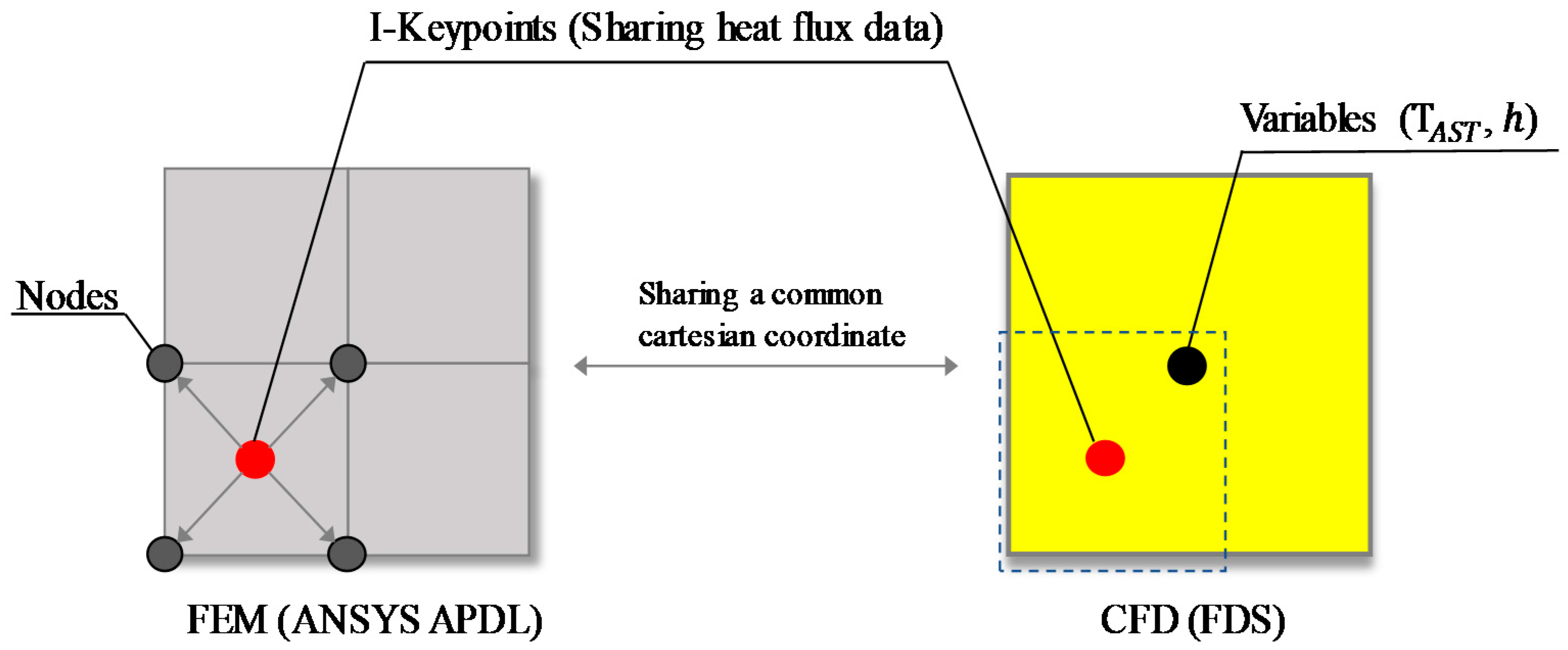
2.3. FTMI Method
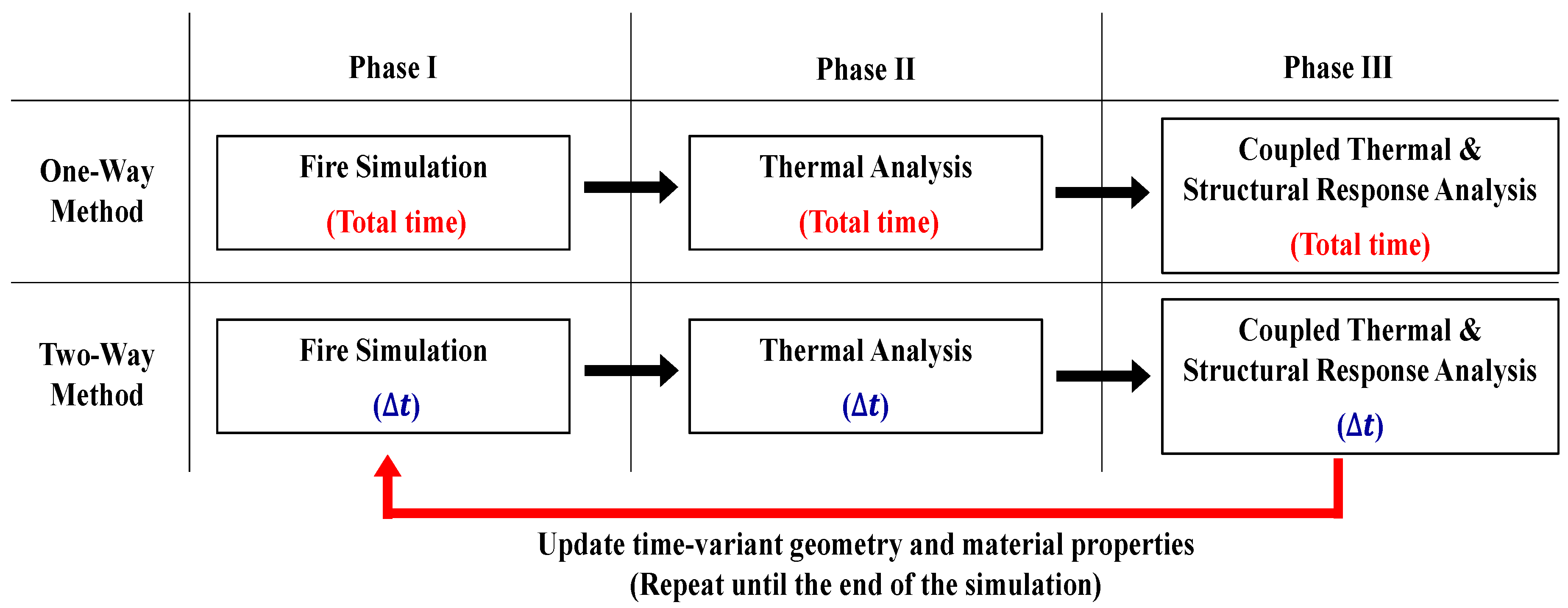
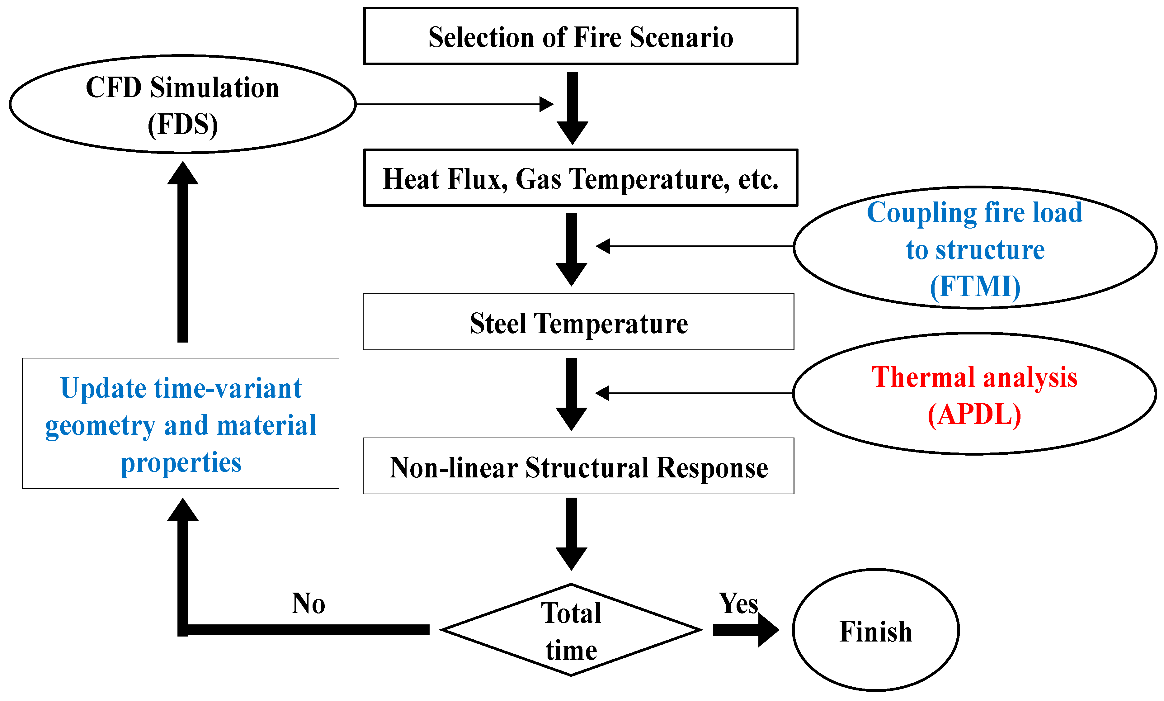
2.4. Numerical Approach for Two-Way FSI
- CFD simulation by using the FDS
- Heat transfer analysis and non-linear FEM according to the CFD simulation results
- CFD simulation until the second , and updating the geometry with the previous non-linear FEM
- Repetition of the CFD simulation with the updated geometry and FEM until completion of the fire scenario
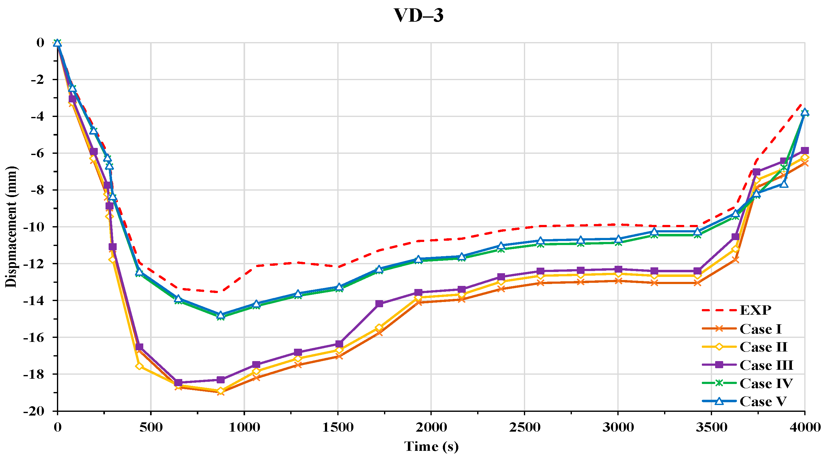
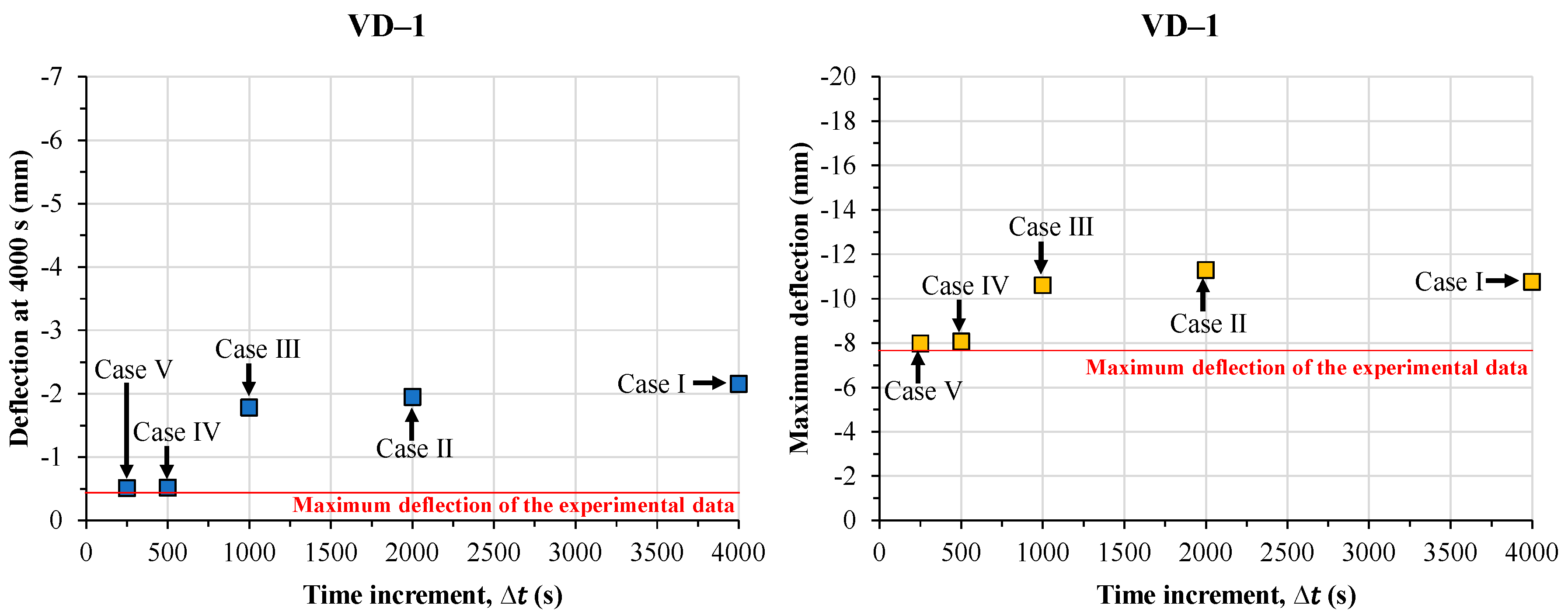
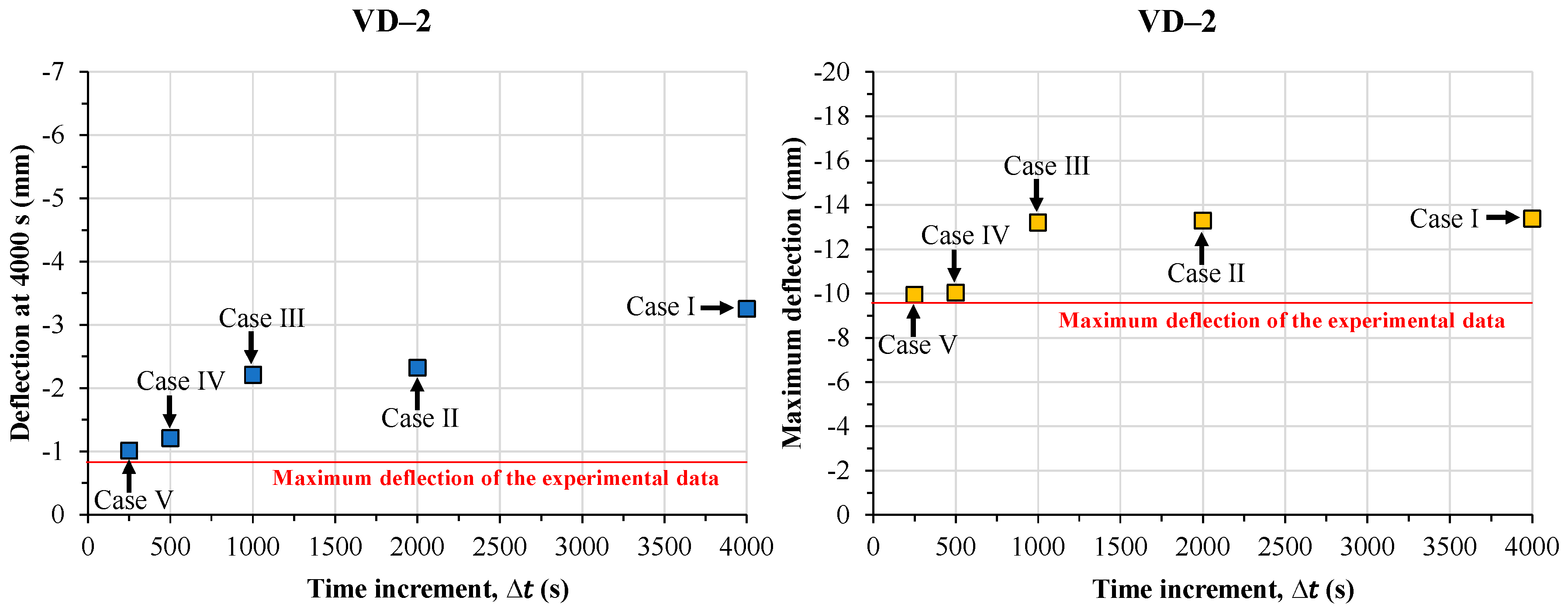
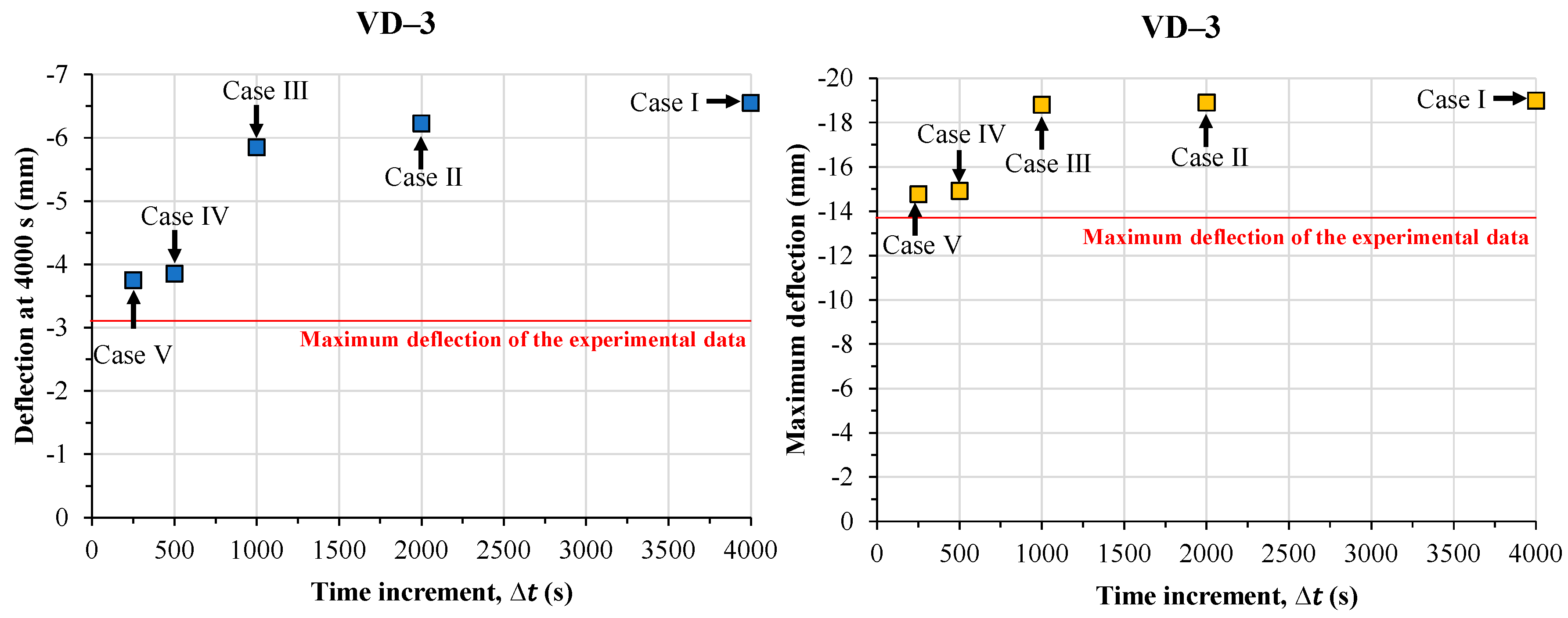
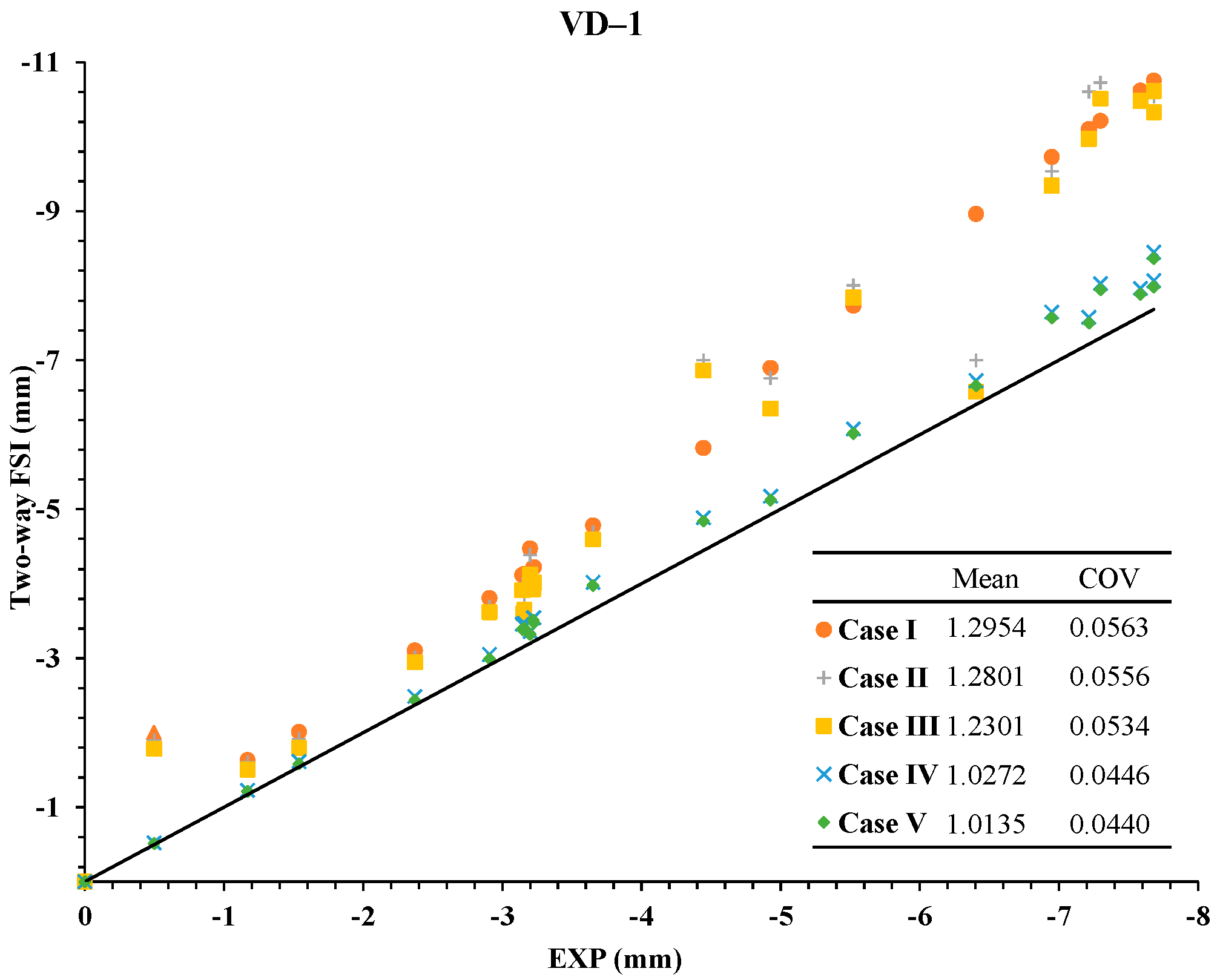
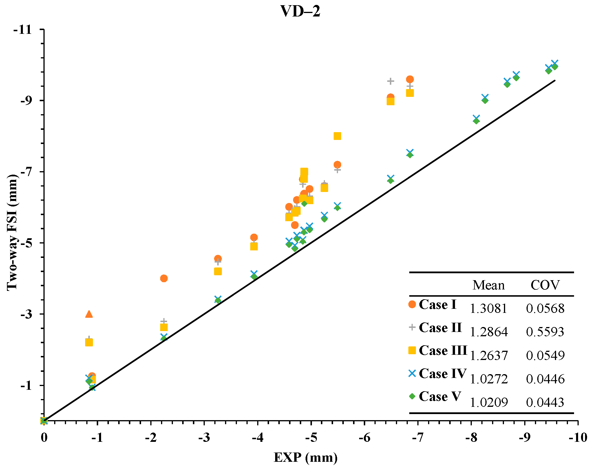
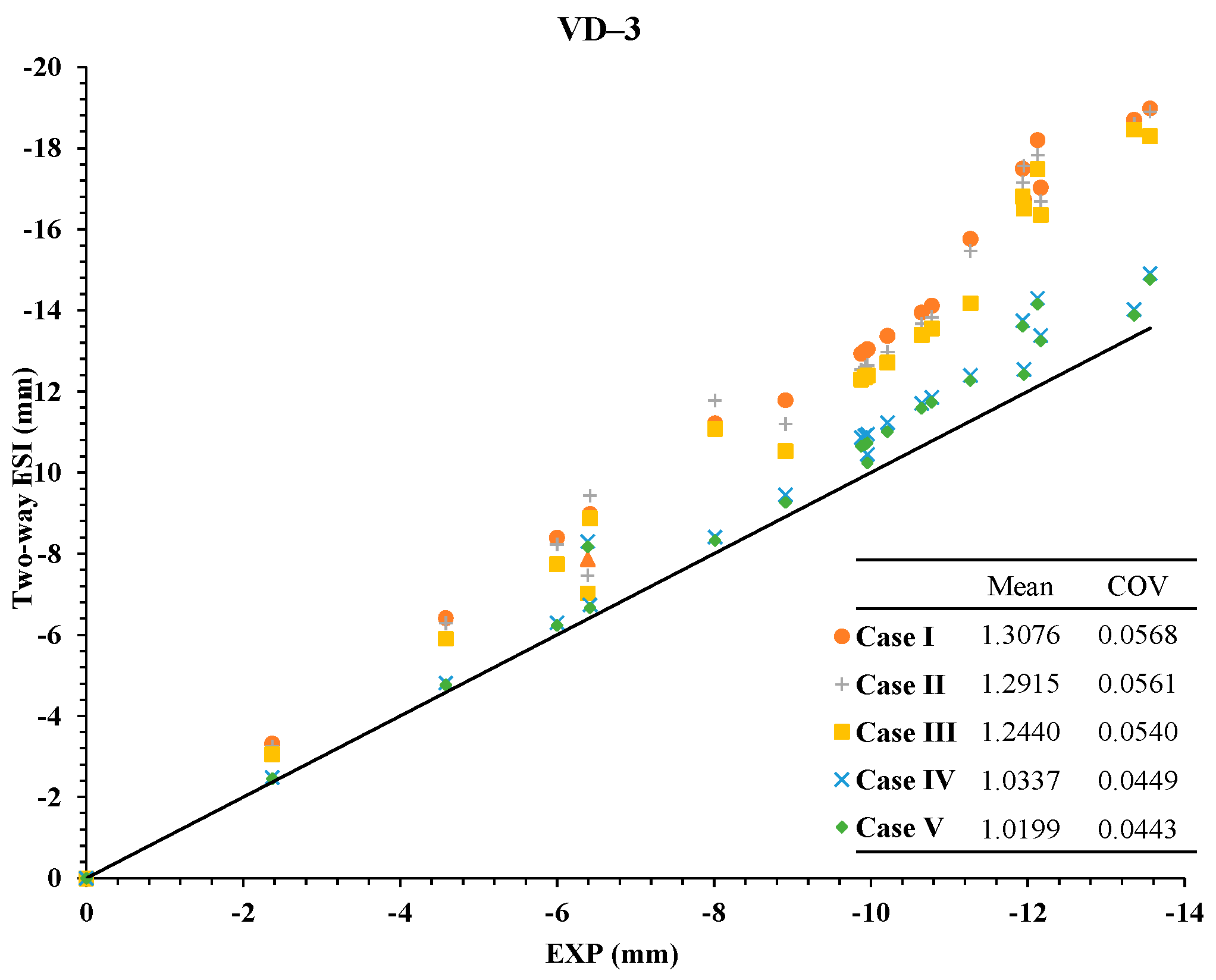
- Case I: 4000 s
- Case II: 2000 s
- Case III: 1000 s
- Case IV: 500 s
- Case V: 250 s
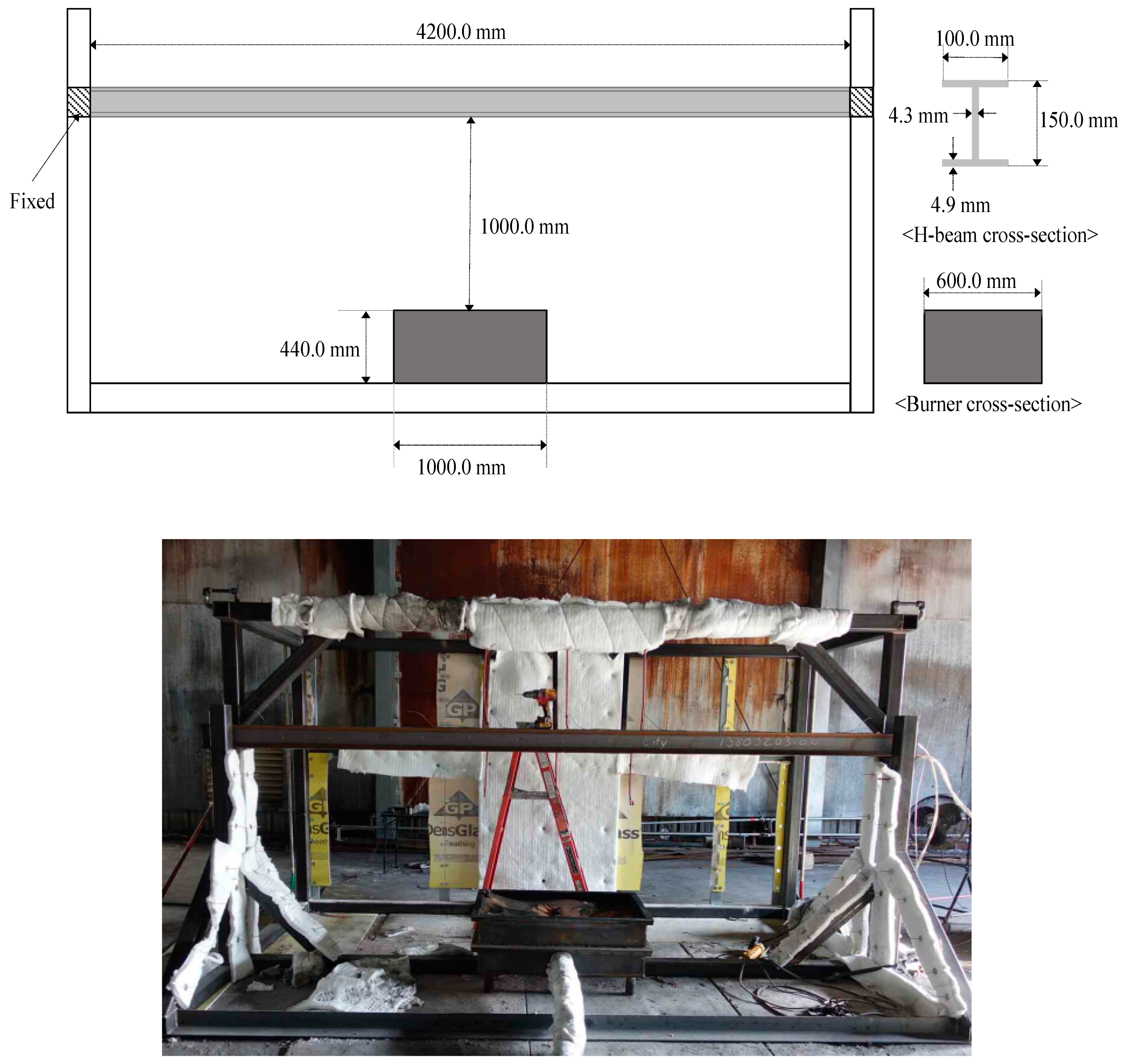
3. Validation Study
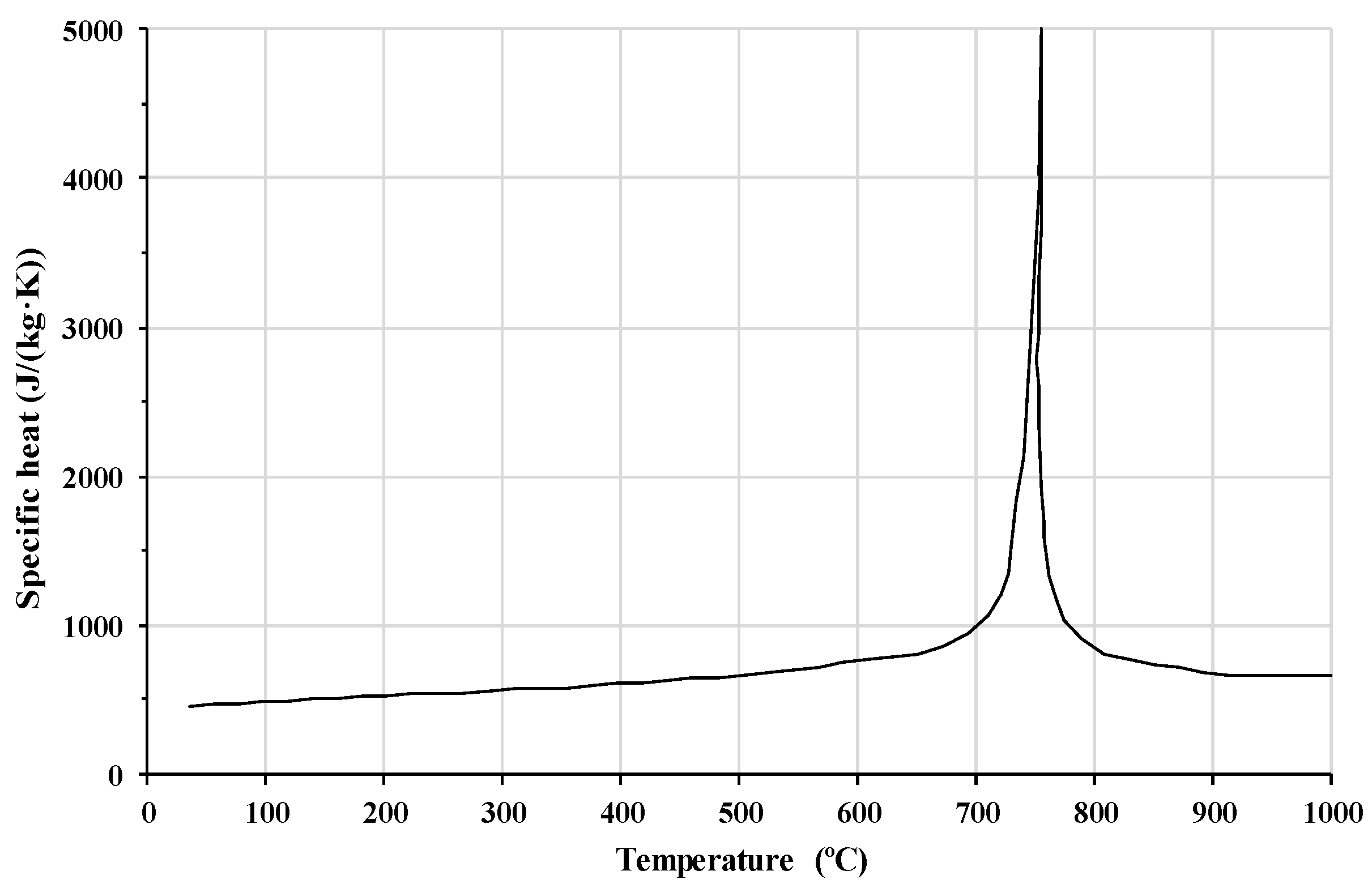
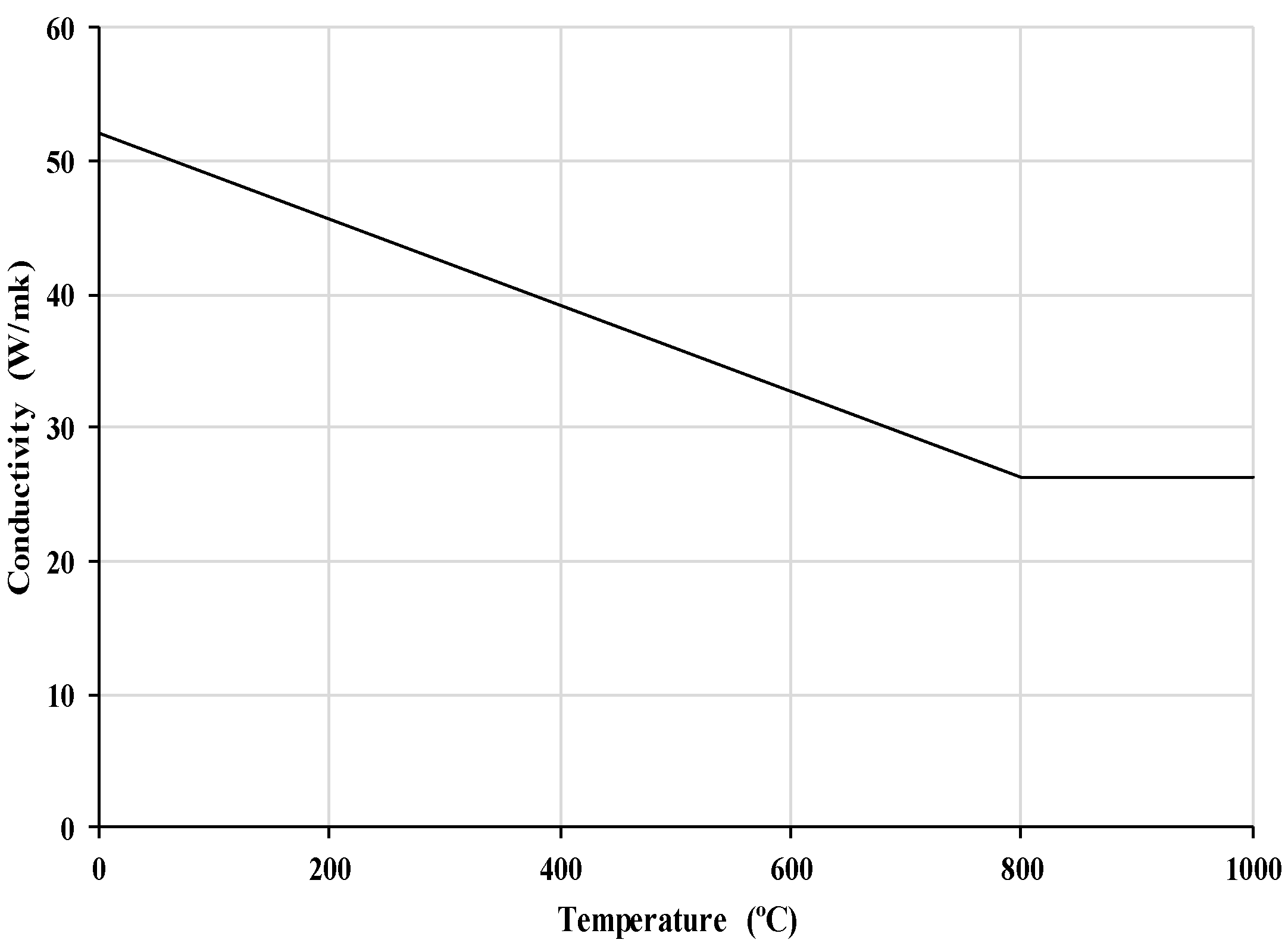
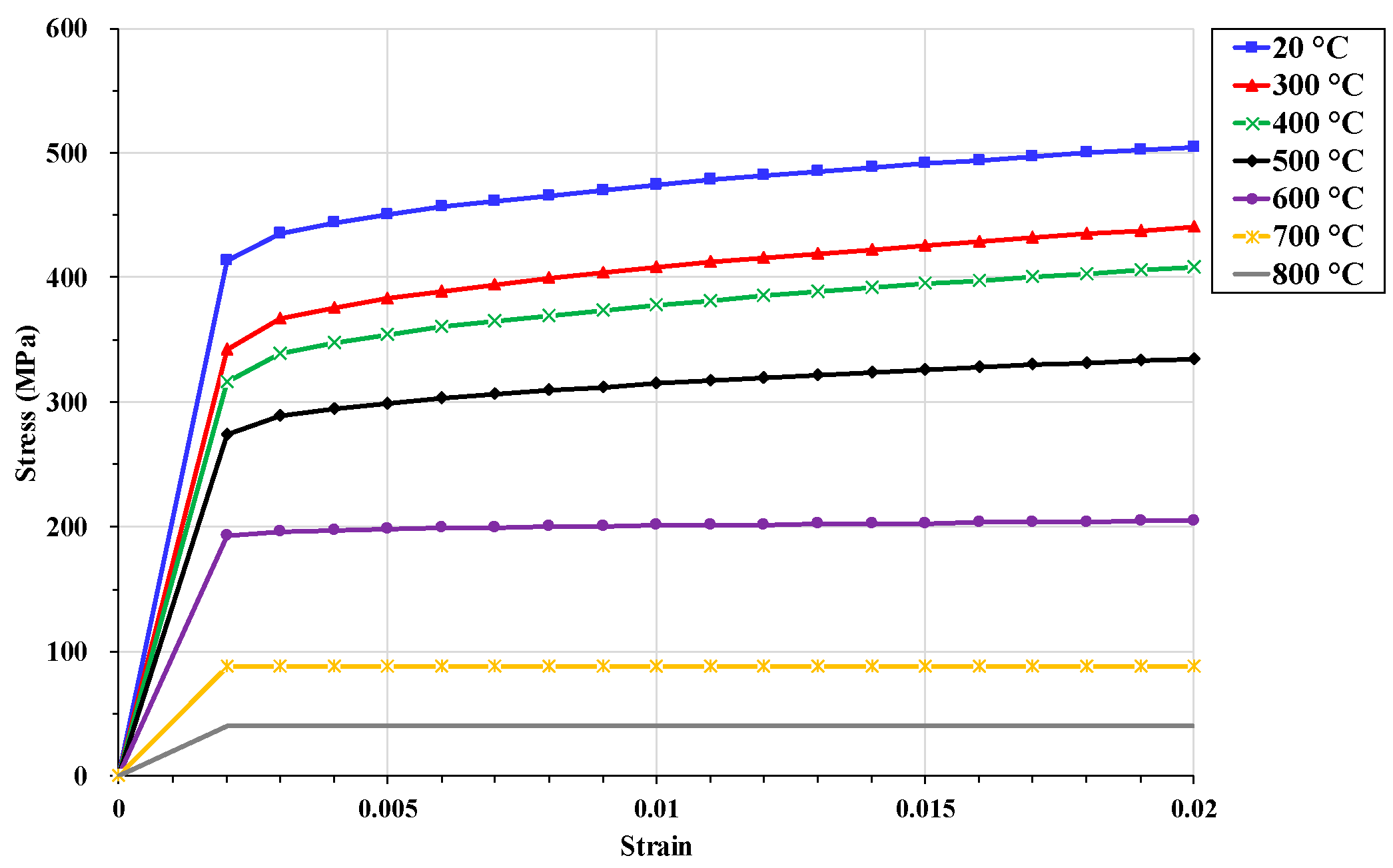
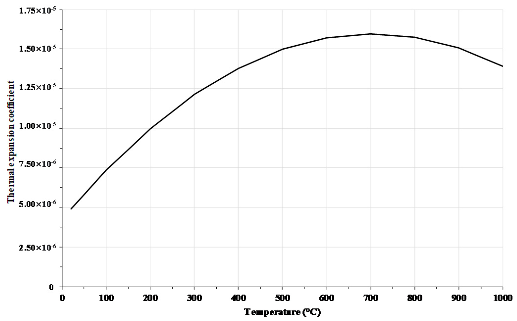
3.1. Material Properties
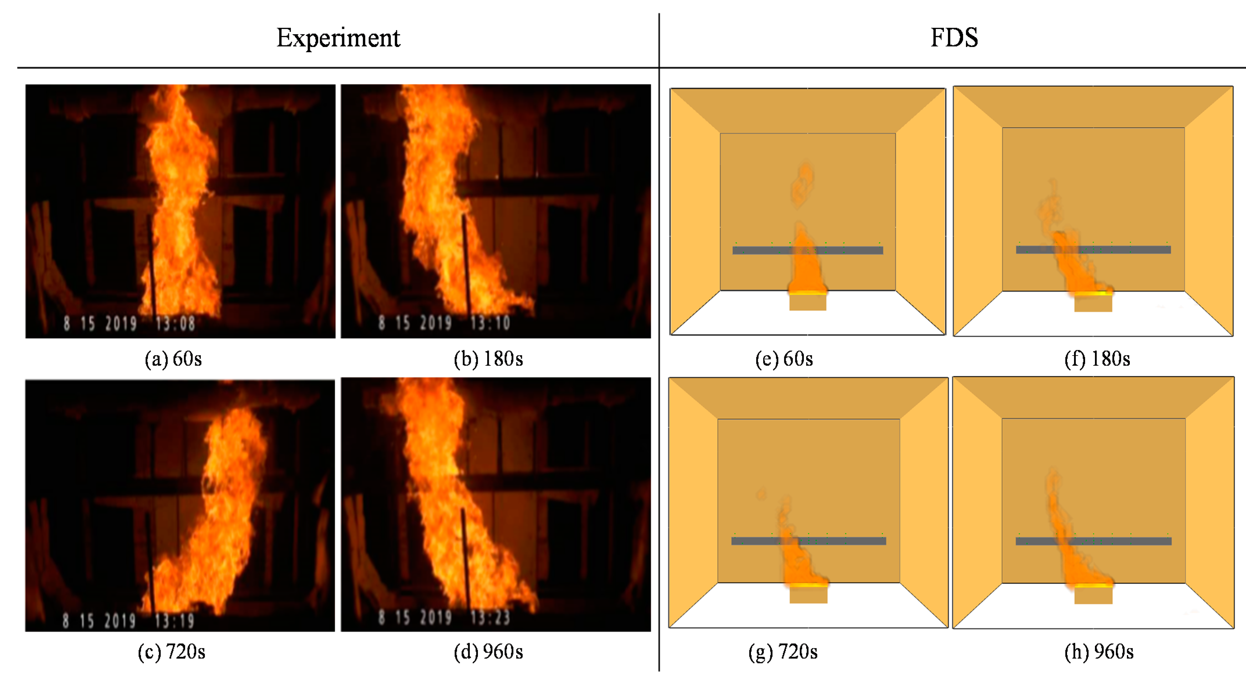
3.2. FDS Simulation of Propane Burner Fire
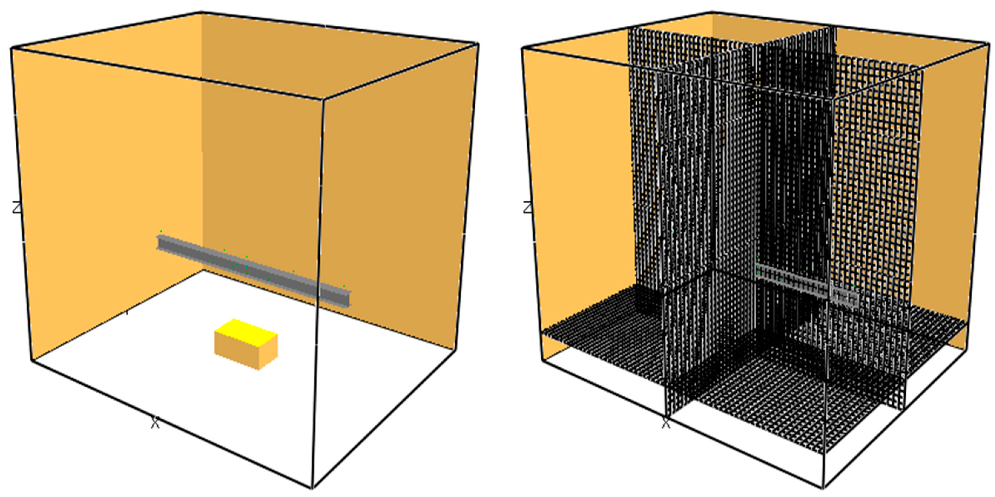
3.2.1. FDS Model Geometry and Computational Mesh
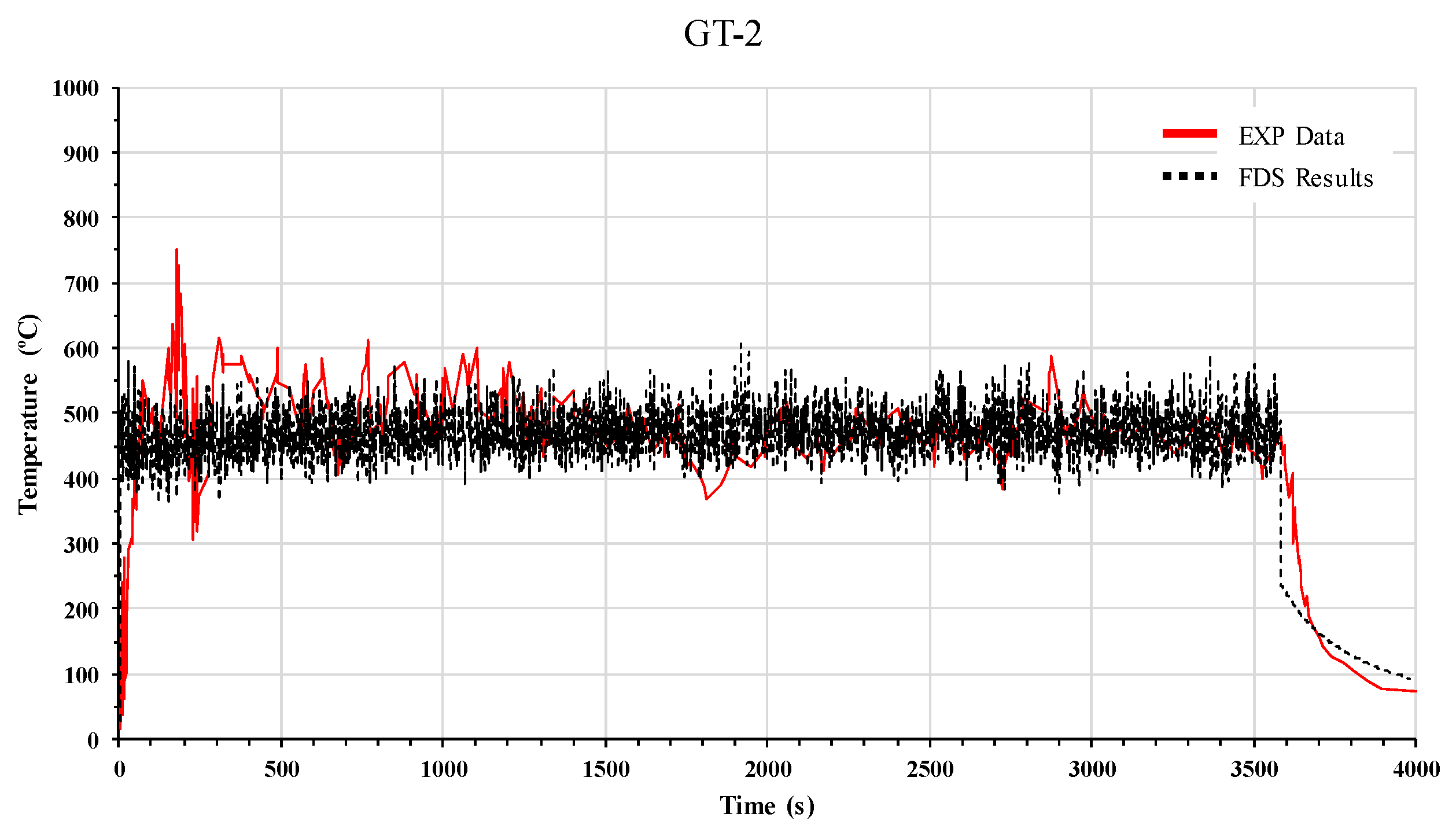
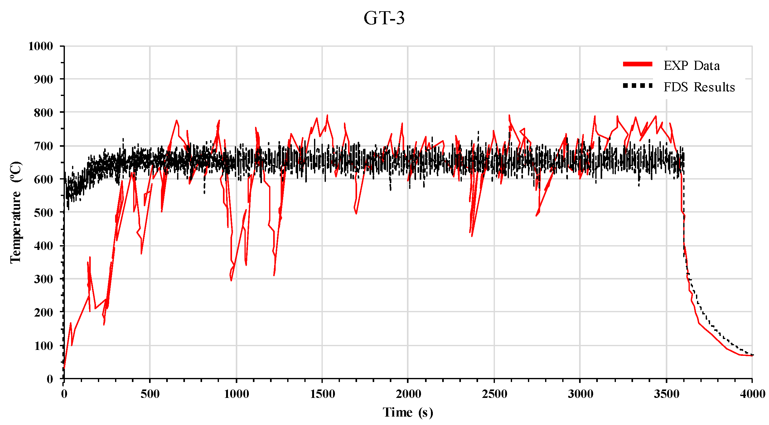
3.2.2. FDS Results and Discussion
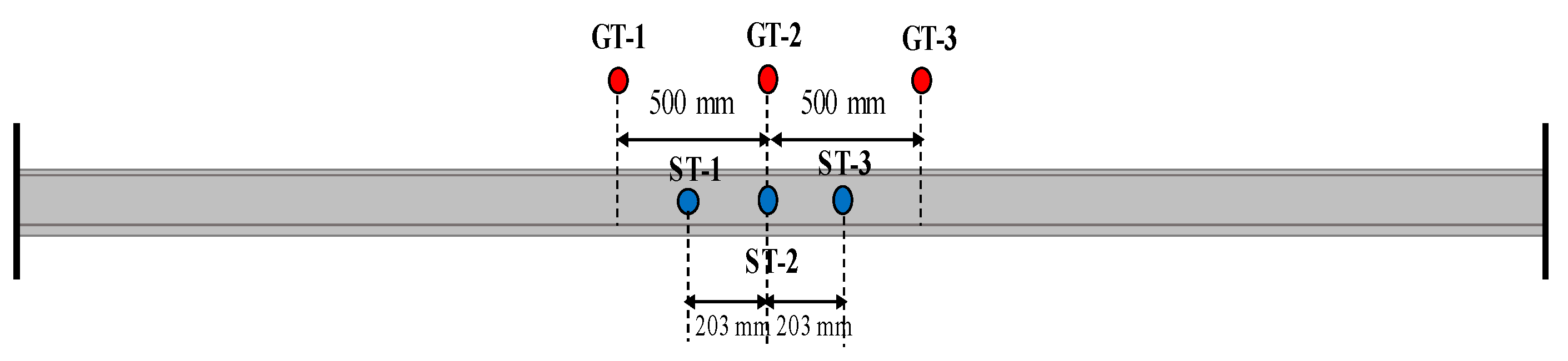
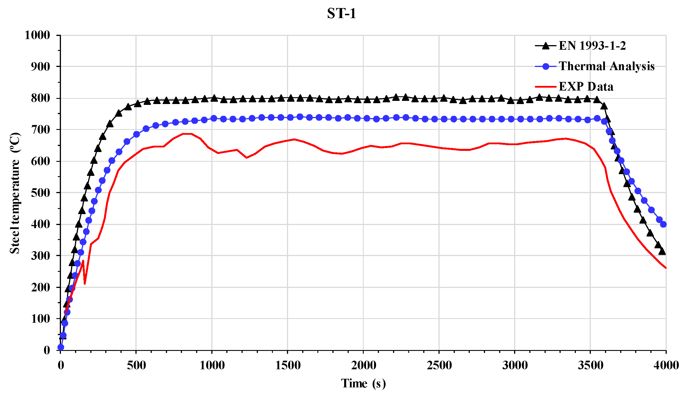
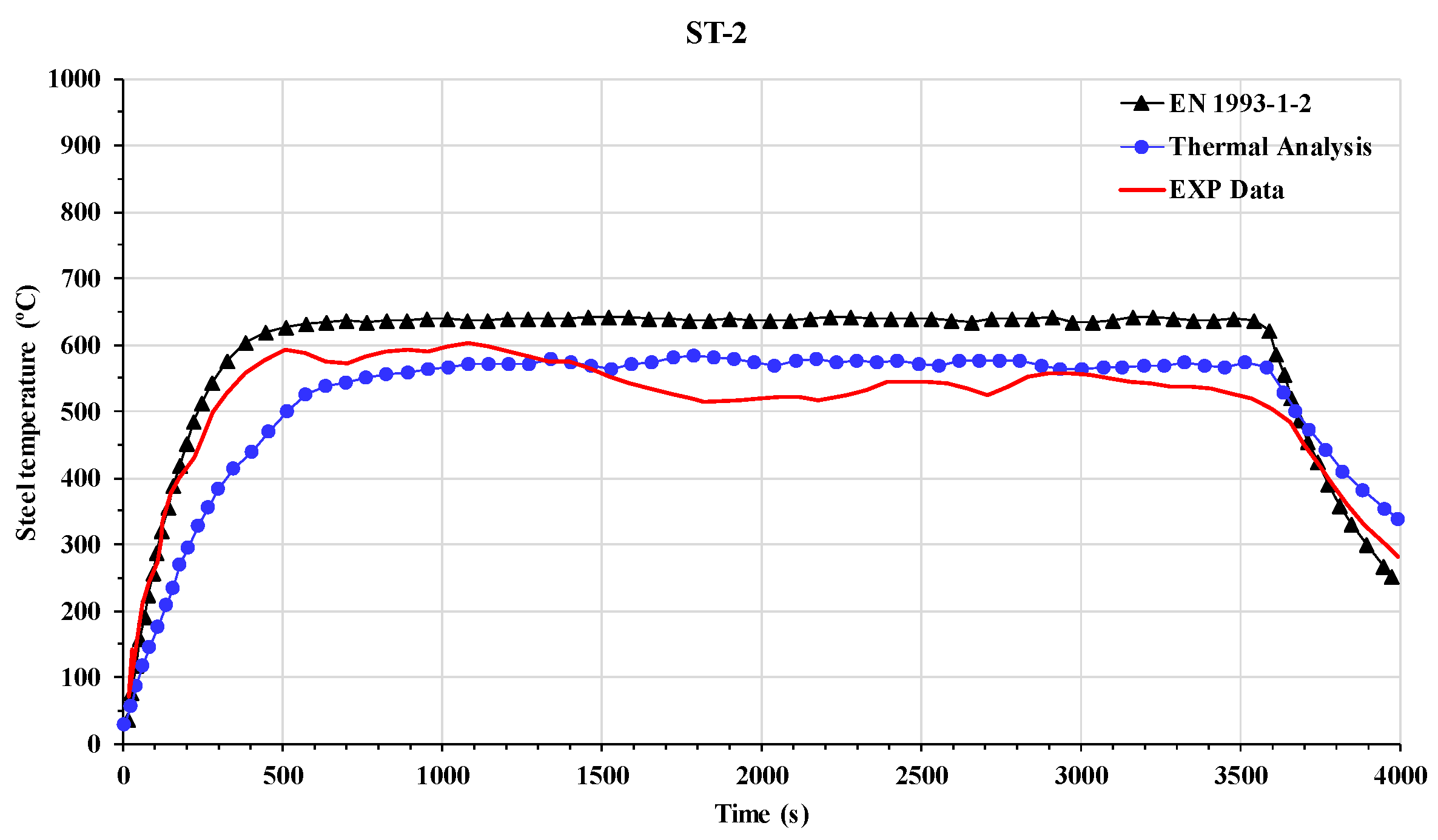
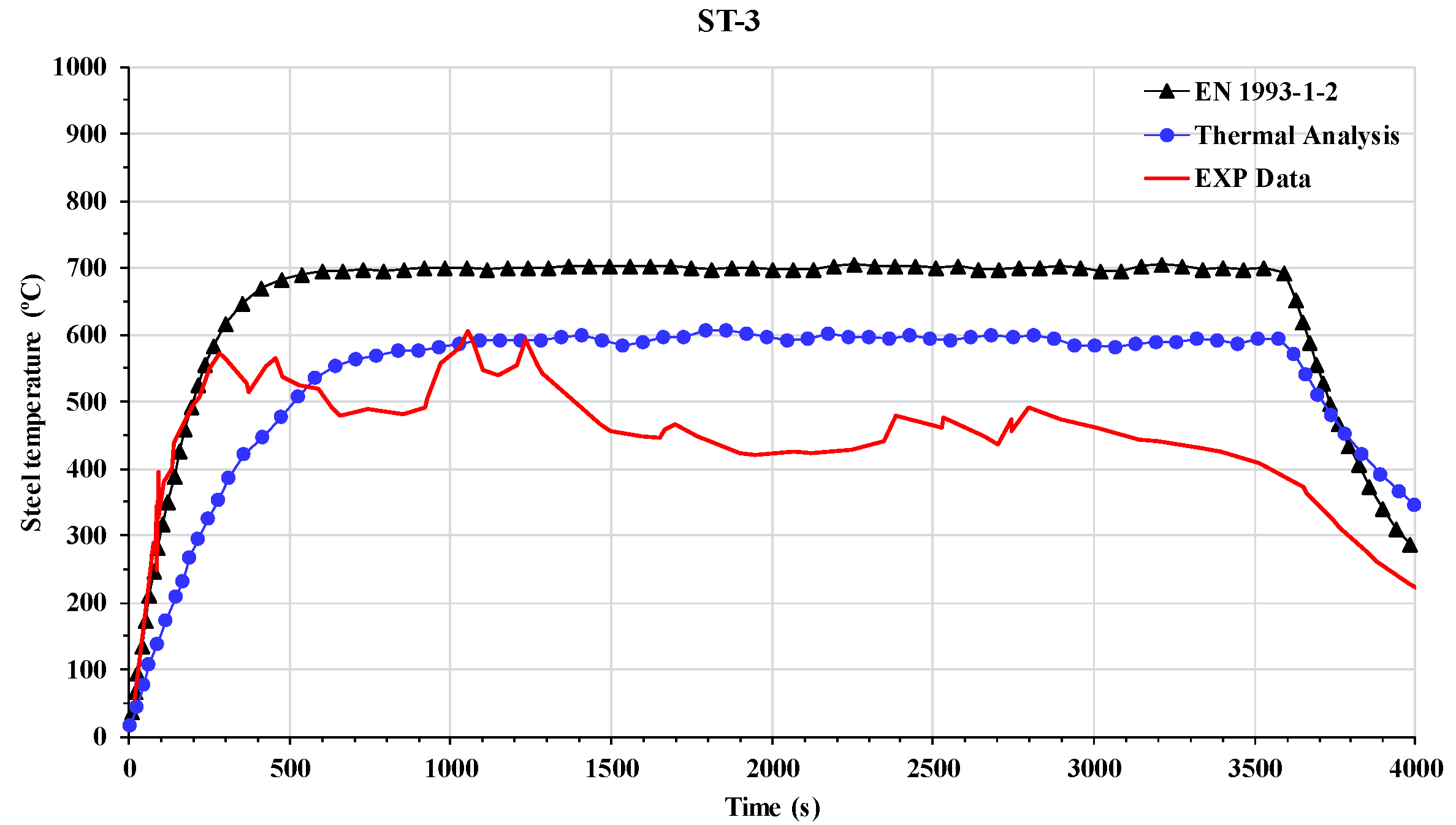
3.3. Thermal Analysis
4. Results and Discussion
5. Conclusions
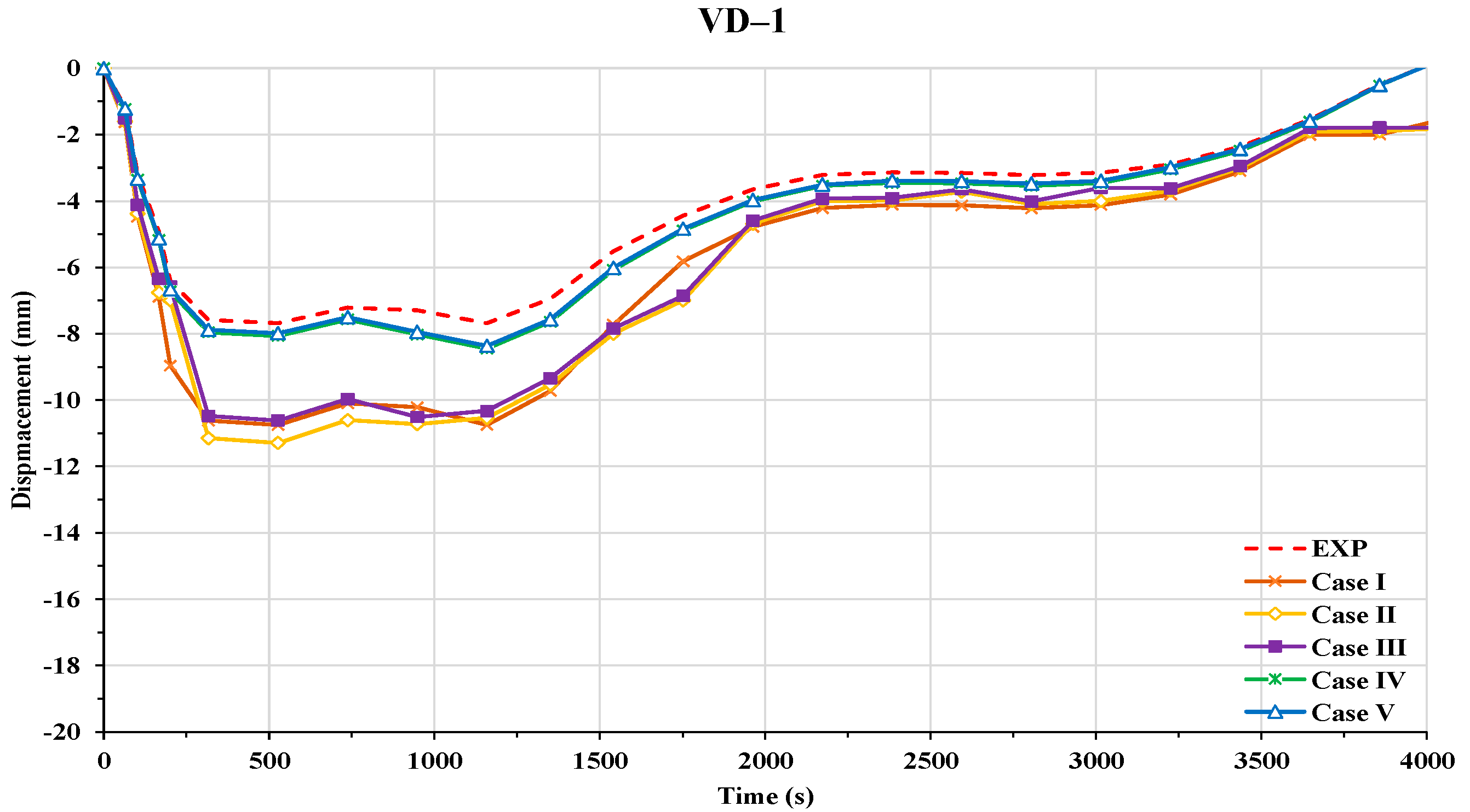
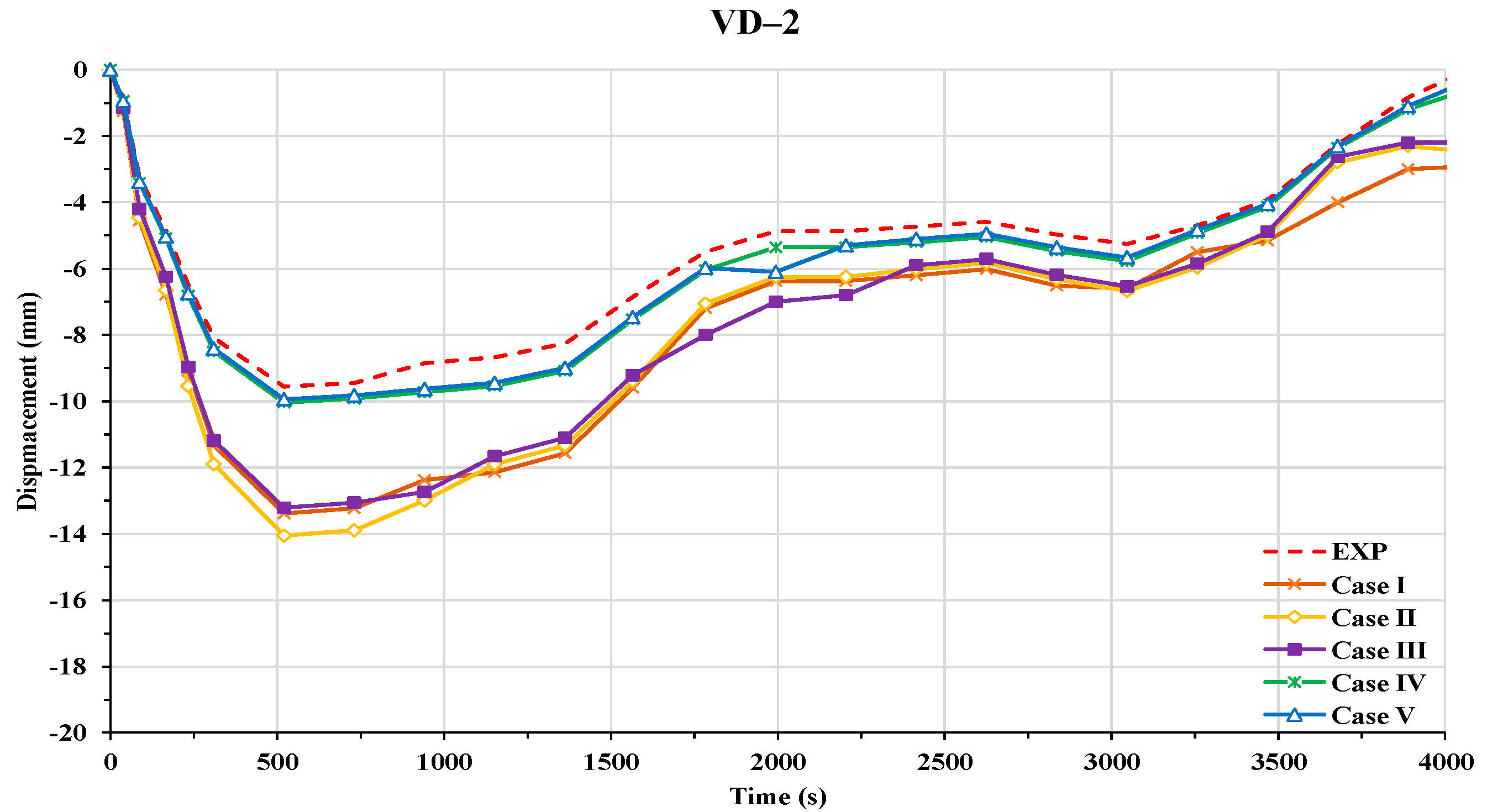
- One-way FSI tended to overestimate the structural consequences of exposing an H-beam to propane burner fire compared with the experimental results.
- One-way FSI may result in the overestimation of the fire safety design requirements for ships and offshore structures.
- For an H-beam under a propane burner fire, a of 500 s was appropriate for two-way FSI. This use of this also led to a similar structural behavior prediction as that obtained by using a smaller (250 s), both of which were similar to the experimental results.
- As the structural consequences increased over time, the differences between the one-way and two-way FSI methods became more significant. This was a result of the one-way FSI being unable to readjust the fire load characteristics, due to changes in the time-variant geometry.
Author Contributions
Funding
Conflicts of Interest
Nomenclature
| Abbreviation | |
| FSI | Fluid-Structure Interaction |
| FDS | Fire Dynamic Simulator |
| FEM | Finite Element Method |
| CFD | Computational Fluid Dynamics |
| CoV | Coefficient of Variation |
| Symbols | |
| Total heat flux [W/m2] | |
| Radiative heat flux [W/m2] | |
| Convective heat flux [W/m2] | |
| Emissivity | |
| Radiative energy absorbed by the surfaces [J] | |
| Stefan–Boltzmann constant | |
| Gas temperature [°C] | |
| Multiplied by the convective heat transfer coefficient [°C] | |
| Convective heat transfer coefficient [W/(m2 K)] | |
| Adiabatic surface temperature [°C] | |
| Increment time [s] | |
| Elastic modulus of steel at room temperature [GPa] | |
| Elastic modulus of steel at elevated temperature [GPa] | |
| Yield strengths of steel at room temperature [MPa] | |
| Yield strengths of steel at elevated temperature [MPa] | |
| Expansion coefficient [1/K] | |
| Diameter of a plume [m] | |
| Heat release rate [W] | |
| Ambient density [ kg/m3] | |
| Specific heat of air at constant pressure [kJ/kg·K] | |
| Length of a grid cell [m] | |
| Spatial resolution | |
| Surface temperature of the steel member [°C] | |
| Correction factor for the shadow effect | |
| Section factor for the unprotected steel member [m−1] | |
| Specific heat of steel [kJ/kg·K] | |
| Mass density of steel [kg/m3] | |
| Net heat flux [W/m2] | |
References
- Paik, J.K.; Czujko, J.; Kim, B.J.; Seo, J.K.; Ryu, H.S.; Ha, Y.C.; Janiszewski, P.; Musial, B. Quantitative assessment of hydrocarbon explosion and fire risks in offshore installations. Mar. Struct. 2011, 24, 73–96. [Google Scholar] [CrossRef]
- Vinnem, J.E. Offshore Risk Assessment; Springer: Dordrecht, The Netherlands, 1999. [Google Scholar]
- Liping, Y.; Zhang, M.; Zhang, Y.; Fangli, Q. Sanchi collision in the East China Sea. Acta Oceanol. Sin. 2018, 37, 69–72. [Google Scholar]
- Zhang, C.; Silva, J.G.; Weinschenk, C.G.; Kamikawa, D.; Hasemi, Y. Simulation Methodology for Coupled Fire-Structure Analysis: Modeling Localized Fire Tests on a Steel Column. Fire Technol. 2016, 52, 239–262. [Google Scholar] [CrossRef]
- Lamont, S.; Lane, B.; Usmani, A. The Behaviour of Multi-storey Composite Steel Framed Structures in Response to Compartment Fires. Fire Saf. Sci. 2005, 8, 177–188. [Google Scholar] [CrossRef]
- Bisby, L.; Gales, J.; Maluk, C. A contemporary review of large-scale non-standard structural fire testing. Fire Sci. Rev. 2013, 2, 1. [Google Scholar] [CrossRef]
- Paik, J.K.; Kim, B.J.; Jeong, J.S.; Kim, S.H.; Jang, Y.S.; Kim, G.S.; Woo, J.H.; Kim, Y.S.; Chun, M.J.; Shin, Y.S.; et al. CFD simulations of gas explosion and fire actions. Ships Offshore Struct. 2010, 5, 3–12. [Google Scholar] [CrossRef]
- Salem, A. Fire engineering tools used in consequence analysis. Ships Offshore Struct. 2010, 5, 155–187. [Google Scholar] [CrossRef]
- Shetty, N.; Soares, C.G.; Thoft-Christensen, P.; Jensen, F. Fire safety assessment and optimal design of passive fire protection for offshore structures. Reliab. Eng. Syst. Saf. 1998, 61, 139–149. [Google Scholar] [CrossRef]
- Soares, C.G.; Teixeira, A. Strength of plates subjected to localized heat loads. J. Constr. Steel Res. 2000, 53, 335–358. [Google Scholar] [CrossRef]
- Bernardi, P.; Michelini, E.; Sirico, A.; Rainieri, S.; Corradi, C. Simulation methodology for the assessment of the structural safety of concrete tunnel linings based on CFD fire—FE thermo-mechanical analysis: A case study. Eng. Struct. 2020, 225, 111193. [Google Scholar] [CrossRef]
- Sun, L.; Yan, H.; Liu, S.; Bai, Y. Load characteristics in process modules of offshore platforms under jet fire: The numerical study. J. Loss Prev. Process. Ind. 2017, 47, 29–40. [Google Scholar] [CrossRef]
- Novozhilov, V. Computational fluid dynamics modeling of compartment fires. Prog. Energy Combust. Sci. 2001, 27, 611–666. [Google Scholar] [CrossRef]
- McGrattan, K.; Hostikka, S.; McDermott, R.; Floyd, J.; Weinschenk, C.; Overholt, K. Fire Dynamics Simulator User’s Guide; VTT Technical Research Centre of Finland: Esbo, Finland, 2013. [Google Scholar]
- Brohez, S.; Caravita, I. Fire induced pressure in airthigh houses: Experiments and FDS validation. Fire Saf. J. 2020, 114, 103008. [Google Scholar] [CrossRef]
- Cicione, A.; Beshir, M.; Walls, R.S.; Rush, D. Full-Scale Informal Settlement Dwelling Fire Experiments and Development of Numerical Models. Fire Technol. 2019, 56, 639–672. [Google Scholar] [CrossRef]
- Rahmani, A.; Salem, M. Simulation of Fire in Super High-Rise Hospitals Using Fire Dynamics Simulator (FDS). Electron. J. Gen. Med. 2020, 17, em200. [Google Scholar] [CrossRef]
- Suh, H.W.; Im, S.M.; Park, T.H.; Kim, H.J.; Kim, H.S.; Choi, H.K.; Chung, J.H.; Bae, S.C. Fire spread of thermal insulation materials in the ceiling of piloti-type structure: Comparison of numerical simulation and experimental fire tests using small- and real-scale models. Sustainability 2019, 11, 3389. [Google Scholar] [CrossRef]
- Zong, L.; Wang, Y.; Wu, B. Risk assessment framework for fire accidents in the ship engine room. In Proceedings of the 2017 4th International Conference on Transportation Information and Safety, Banff, AB, Canada, 8–10 August 2017; pp. 1093–1098. [Google Scholar]
- Jahn, W.; Rein, G.; Torero, J.L. A posteriori modelling of the growth phase of Dalmarnock Fire Test One. Build. Environ. 2011, 46, 1065–1073. [Google Scholar] [CrossRef]
- Zhang, C.; Li, G.Q. Fire dynamic simulation on thermal actions in localized fires in large enclosure. Adv. Steel Constr. 2012, 8, 124–136. [Google Scholar] [CrossRef]
- Wen, J.; Kang, K.; Donchev, T.; Karwatzki, J. Validation of FDS for the prediction of medium-scale pool fires. Fire Saf. J. 2007, 42, 127–138. [Google Scholar] [CrossRef]
- Prasad, K.; Baum, H.R. Coupled fire dynamics and thermal response of complex building structures. Proc. Combust. Inst. 2005, 30, 2255–2262. [Google Scholar] [CrossRef]
- Zhang, C.; Li, G.Q. Thermal Response of Steel Columns Exposed to Localized Fires-Numerical Simulation and Comparison with Experimental Results. J. Struct. Fire Eng. 2011, 2, 311–318. [Google Scholar] [CrossRef]
- Chen, L.; Luo, C.; Lua, J. FDS and abaqus coupling toolkit for fire simulation and thermal and mass flow prediction. Fire Saf. Sci. 2011, 10, 1465–1477. [Google Scholar] [CrossRef]
- Alos-Moya, J.; Paya-Zaforteza, I.; Garlock, M.; Loma-Ossorio, E.; Schiffner, D.; Hospitaler, A. Analysis of a bridge failure due to fire using computational fluid dynamics and finite element models. Eng. Struct. 2014, 68, 96–110. [Google Scholar] [CrossRef]
- Silva, J.C.G.; Landesmann, A.; Ribeiro, F.L.B. Fire-thermomechanical interface model for performance-based analysis of structures exposed to fire. Fire Saf. J. 2016, 83, 66–78. [Google Scholar] [CrossRef]
- Kim, S.J.; Lee, J.; Kim, S.H.; Seo, J.K.; Kim, B.J.; Ha, Y.C.; Paik, J.K.; Lee, K.S.; Park, B.; Ki, M.S.; et al. Nonlinear structural response in jet fire in association with the interaction between fire loads and time-variant geometry and material properties. Ocean Eng. 2017, 144, 118–134. [Google Scholar] [CrossRef][Green Version]
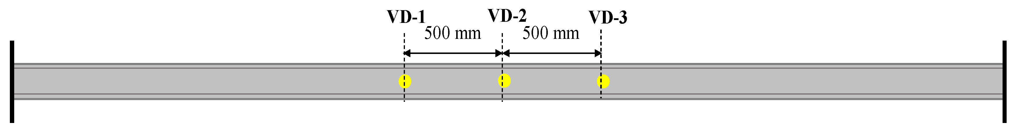
- Ki, M.S.; Park, B.J.; Lee, K.; Park, B.; Fernandez, K.; Nho, I.S. An Experimental Study on the H-Beam Under Fire Load in Open Space. J. Ocean Eng. Technol. 2021, 35, 59–74. [Google Scholar] [CrossRef]
- European Committee for Standardization. EN 1993-1-2: Eurocode 3: Design of Steel Structures: Part 1–2: General Rules-Structural Fire Design; European Committee for Standardization: Brussels, Belgium, 2005. [Google Scholar]
- Wickström, U. Heat transfer by radiation and convection in fire testing. Fire Mater. 2004, 28, 411–415. [Google Scholar] [CrossRef]
- Wickström, U.; Duthinh, D.; McGrattan, K. Adiabatic surface temperature for calculating heat transfer to fire exposed structures. In Proceedings of the 11th International Interflam Conference, London, UK, 3–5 September 2005. [Google Scholar]
- Shen, T.S.; Huang, Y.H.; Chien, S.W. Using fire dynamic simulation (FDS) to reconstruct an arson fire scene. Build. Environ. 2008, 43, 1036–1045. [Google Scholar] [CrossRef]
- Duthinh, D.; McGrattan, K.; Khaskia, A. Recent advances in fire: Structure analysis. Fire Saf. J. 2008, 43, 161–167. [Google Scholar] [CrossRef][Green Version]
- Sandström, J.; Wickström, U.; Veljkovic, M. Adiabatic surface temperature: A sufficient input data for a thermal model. In Application of Structural Fire Engineering; 19/02/2009–20/02/2009; Czech Technical University in Prague: Prague, Czech Republic, 2009. [Google Scholar]
- Luecke, W.; Banovic, S.W.; McColskey, J.D. High-Temperature Tensile Constitutive Data and Models for Structural Steels in Fire; NIST Technical Note 1714; National Institute of Standards and Technology: Gaithersburg, MD, USA, 2015. [Google Scholar]


Publisher’s Note: MDPI stays neutral with regard to jurisdictional claims in published maps and institutional affiliations. |
© 2021 by the authors. Licensee MDPI, Basel, Switzerland. This article is an open access article distributed under the terms and conditions of the Creative Commons Attribution (CC BY) license (https://creativecommons.org/licenses/by/4.0/).
Share and Cite
Woo, D.; Seo, J.K. Numerical Validation of the Two-Way Fluid-Structure Interaction Method for Non-Linear Structural Analysis under Fire Conditions. J. Mar. Sci. Eng. 2021, 9, 400. https://doi.org/10.3390/jmse9040400
Woo D, Seo JK. Numerical Validation of the Two-Way Fluid-Structure Interaction Method for Non-Linear Structural Analysis under Fire Conditions. Journal of Marine Science and Engineering. 2021; 9(4):400. https://doi.org/10.3390/jmse9040400
Chicago/Turabian StyleWoo, Donghan, and Jung Kwan Seo. 2021. "Numerical Validation of the Two-Way Fluid-Structure Interaction Method for Non-Linear Structural Analysis under Fire Conditions" Journal of Marine Science and Engineering 9, no. 4: 400. https://doi.org/10.3390/jmse9040400
APA StyleWoo, D., & Seo, J. K. (2021). Numerical Validation of the Two-Way Fluid-Structure Interaction Method for Non-Linear Structural Analysis under Fire Conditions. Journal of Marine Science and Engineering, 9(4), 400. https://doi.org/10.3390/jmse9040400