Article

Optimal Actuator Placement for Real-Time Hybrid Model Testing Using Cable-Driven Parallel Robots

1
Centre for Autonomous Marine Operations and Systems (NTNU AMOS), Department of Marine Technology, Norwegian University of Science and Technology, NO-7491 Trondheim, Norway
2
SINTEF Ocean, NO-7465 Trondheim, Norway
*
Author to whom correspondence should be addressed.
J. Mar. Sci. Eng. 2021, 9(2), 191; https://doi.org/10.3390/jmse9020191
Submission received: 11 January 2021 / Revised: 2 February 2021 / Accepted: 8 February 2021 / Published: 12 February 2021
(This article belongs to the Special Issue Waves and Ocean Structures II)

Abstract

:
In real-time hybrid model testing, complex ocean structures are emulated by fusing numerical modelling with traditional hydrodynamic model testing. This is done by partitioning the ocean structure under consideration into a numerical and a physical substructure, coupled in real time via a measurement and control interface. The numerically computed load vector is applied to the physical substructure by means of multiple actuated winches so that the resulting experimental platform becomes a type of cable-driven parallel robot. In this context, the placement of the actuated winches is important to ensure that the loads can be accurately and robustly transferred to the physical substructure. This paper addresses this problem by proposing a performance measure and an associated actuator placement procedure that enables accurate force tracking and ensures that the numerically calculated loads can be actuated throughout the testing campaign. To clarify the application of the proposed procedure, it is applied to the design of a test setup for a moored barge. Overall, the paper represents a guideline for robust and beneficial actuator placement for real-time hybrid model testing using cable-driven parallel robots for load-actuation.

1. Introduction

Real-time hybrid model testing (ReaTHM testing) is a cyber-physical empirical method for emulating complex ocean structures that combines numerical models with traditional hydrodynamic model testing [1,2]. This is done by partitioning the ocean structure under consideration into a numerical substructure and a physical substructure that are coupled in real time through a measurement and control interface. See Figure 1. The method enables emulation of ocean systems where neither a purely numerical simulation nor a purely physical model test is feasible within satisfactory performance levels.
Applications of the method include testing of offshore wind turbines [3]—to overcome the Froude-Reynolds scaling conflict [4], seakeeping tests of floating structures [5]—to overcome limitations of soft horizontal mooring systems, and testing of moored structures [6]—to overcome spacial limitations of ocean basin laboratories (see Figure 2). In the above-cited applications, and in line with the present publication, the numerically calculated load vector is transferred to the physical substructure using multiple actuated winches. Thus, the resulting experimental substructure becomes a type of cable-driven parallel robot (CDPR), which is a setup characterised by a mobile platform being actuated by cabled winches configured in a parallel topology [7]. See Figure 3. From each cabled actuator, the actuated load is a function of the cable-tension and its two cable endpoints. Due to actuator limitations and to avoid slack cables, lower and upper constraints are enforced on the cable-tensions. the cable endpoints of all connected actuators, together with the platform pose, constitute the platform configuration of a CDPR.
Beyond their use for ReaTHM testing, CDPRs have received considerable attention in recent decades [9,10] for diverse applications, including aerial cameras [11], manufacturing [12], agriculture [13], and ocean engineering [14]. They are recognised for their large workspace coverage, lightweight structure, fast dynamics, and reconfigurability [15,16,17].
In our experience, placement of actuators in previous ReaTHM testing CDPR setups, such as [3,6,8], has mostly been determined using a practical and heuristic approach, i.e., for a given ReaTHM testing scenario, the actuators have been placed based on simplified analysis, experiential experience and intuitive understanding – with limited systematic analysis. At the time of this publication, no guidelines exist for actuator placement for ReaTHM testing using CDPR.
Conversely, for other CDPR applications, the minimization of performance measures evaluating the quality of platform configurations are commonly used to determine the optimal placement of actuators ([10] [Ch 8]). Reference [18] suggests using a controllability measure based on eigenvectors, which is a popular measure when considering the control of linear systems [19]. Also related to controllability, [20,21,22] uses a conditioning number referred to as the platform dexterity measure. Several references [22,23,24] use performance measures related to the CDPR’s stiffness, with the goal of either maximising the stiffness or ensuring that the stiffness distribution is uniform. Reference ([10] [Ch 8]) lists several additional performance measures including quality of tension distribution, accuracy, energy considerations, closeness to singularities, and proximity to cable collision. Other popular performance measures relate to optimising workspace coverage. These performance measures can for example be to maximise the range of poses in which certain prescribed loads can be actuated [25,26] (wrench-feasible workspace), or the range of poses for which any load can be actuated given no upper cable-tension constraints [27] (wrench-closure workspace).
In some cases, the performance measure is minimised subject to specific requirements being satisfied. See for example [28] in which actuator placement is determined by minimising cable tensions subject to the condition that wrench-closure workspace requirements are satisfied. In [29] the search for optimal actuator placement is divided into an exploration phase, in which promising CDPR geometries are identified, and a subsequent optimisation phase, in which the optimal actuator placement is determined by minimising the proposed performance measure for the selected geometries.
In ReaTHM testing, precisely applying the calculated loads onto the marine platform is particularly important to achieve high fidelity in replicating the non-substructured ocean structure’s behaviour [8,30,31]. Although there are many performance measures for CDPR setups, these are in our opinion, not appropriate for ReaTHM testing—as this application requires a different set of priorities, as elaborated next.
Table 1 lists characteristic differences between CDPR used in ReaTHM testing [2,6,8] and typical1 CDPR setups used for other applications ([10] [Ch 2.4]). the practical implications of these differences are as follows:
  • Whereas there is some margin for load (forces and moments) tracking errors in typical CDPR applications, accurate load tracking is paramount to ensure high-fidelity ReaTHM testing [31]. Therefore, the relative focus on accurate load control is considerably higher for the latter.
  • For typical CDPR applications, a higher stiffness throughout the workspace may be preferable to minimise undesired perturbations from external disturbances [24]. Conversely, for ReaTHM testing, a lower stiffness is preferable, to make the setup less sensitive to platform motions (this relates to delay-induced errors, as discussed in [32]).
  • Given similar platform dimensions, the actuation system in typical CDPR applications carries larger loads than in ReaTHM testing and must be designed accordingly.
  • In ReaTHM testing, the platform design is fixed to the emulation target, whereas in typical CDPR applications multiple platform designs may serve the same purpose.
These items imply a different focus when determining the actuator placement for the two cases. For ReaTHM testing, we propose using a procedure that aims at accurate load actuation—while ensuring that the target load vector is always achievable. Conversely, actuator placement for typical CDPR applications is not based on load actuation accuracy, but on other measures [10,20,21,22,25,26], as discussed earlier.
In this paper, we seek to develop a procedure for placement of actuators for CDPR setups that is suitable for use in ReaTHM testing. Specifically, we seek a procedure for placement of actuators that: (1) facilitates accurate load tracking—which is important to ensure high fidelity ReaTHM testing that accurately predicts the behaviour of the target ocean structure, and (2) ensures that the actuators can always actuate the numerically calculated loads according to specified workspace requirements—which is a prerequisite to carry out a successful ReaTHM testing campaign. the resulting procedure shall be optimal in the sense that it minimises the proposed performance measure.
The remainder of the paper is structured as follows. Section 2 outlines the preliminary background. Section 3 presents the proposed procedure for actuator placement. Section 4 demonstrates the procedure for ReaTHM testing of a moored barge.

2. Problem Formulation

2.1. Force Allocation

Force allocation for CDPR is the problem of finding the optimal cable tensions f * = ( f 1 * , f 2 * , , f n * ) on an overconstrained CDPR setup such that they sum up to the reference load vector w ref R m , where n is the number of connected cabled actuators and m is the number of controlled degrees of freedom (DOF) in which the load w ref shall be actuated. We typically consider the physical platform to be described in 6 DOF, in which case m 6 . In the case of ReaTHM testing w ref corresponds to the numerically calculated load vector that is to be actuated onto the physical substructure. See Figure 1.
We next express the force allocation problem as an optimisation problem, similar to [36]. When considering the experimental setup, we refer to two reference frames, { a } and { b } ; O a is the local Earth-fixed coordinate frame’s stationary origin { a } , and O b is the platform’s body-fixed frame’s moving origin { b } . See Figure 5. Accordingly, vectors decomposed in { a } or { b } are given superscripts a or b, respectively. If the superscript is omitted, and the vector has not been previously defined, then it is decomposed in { a } .
The position and orientation (pose) of the body frame { b } relative to { a } are denoted p : = p a = ( x , y , z ) R 3 and Θ : = ( ϕ , θ , ψ ) S 1 3 , where S 1 [ π , π ) (this paper represents orientation by the z y x Euler angle convention ([37] [Ch 2.2.1])). These are combined in the body’s pose vector η : = ( p , Θ ) R 3 × S 1 3 . For each actuator i { 1 , , n } , let p a i : = p a i a be the fixed position of the i th cable exit point A i . Similarly, let the constant body-fixed lever arm from O b to the i th cable attachment anchor E i (on the platform) be denoted r i b .
The Euler angle rotation matrix R ( Θ ) maps vectors from { b } to { a } :
R ( Θ ) = R z ( ψ ) R y ( θ ) R x ( ϕ ) ,
with,
R x = 1 0 0 0 cos ( ϕ ) sin ( ϕ ) 0 sin ( ϕ ) cos ( ϕ ) , R y = cos ( θ ) 0 sin ( θ ) 0 1 0 sin ( θ ) 0 cos ( θ ) , R z = cos ( ψ ) sin ( ψ ) 0 sin ( ψ ) cos ( ψ ) 0 0 0 1 .
Accordingly, r i a = R ( Θ ) r i b .
It follows that the absolute position of E i is p e i : = p e i a = p + R ( Θ ) r i b . From each actuator i, a force f i directed along the straight line p a i p e i , with direction denoted by the unit vector u i : = p a i p e i | p a i p e i | is actuated on the platform at E i . The relationship between the cable tensions f = ( f 1 , f 2 , , f n ) and the resulting load vector w generated by the cables is described by w = W f , where
W = q 1 q 2 q n ,   with   q i = u i r i a × u i ,
The set of cable attachment points { p a } : = ( p a 1 , p a 2 , , p a n ) combined with the body-fixed lever arms { r b } : = ( r 1 b ,   r 2 b , ,   r n b ) are referred to as the actuator configuration of the CDPR. The platform configuration of the CDPR refers to the actuator configuration combined with the platform pose η , and thus describes the cable endpoints for all actuator cables.
In solving the force allocation problem as an optimisation problem, we find f * as the cable tensions f that minimise a cost function g ( f ) subject to cable constraints f min f f max and kinematic mapping,
f * = arg min f { g ( f ) : f R n , W f = w ref , f min f f max }
where f is any cable tension vector f satisfying the constraints.
In this paper, we will use the following cost function:
g ( f ) = i = 1 n | f i f 0 , i | 2 α 2 c 1 log ( f i f i , min ) c 2 log ( f i , max f i ) ,
where α ,   c 1 and c 2 are scaling parameters and f 0 = ( f 0 , 1 , f 0 , 2 , , f 0 , n ) is the preferred load vector dependent on application specific factors such as actuator technology, cable properties, safety concerns, and operating conditions. The cost function has beneficial properties, as shown in [36].

2.2. The ReaTHM Testing Loop

Figure 6 shows the resulting ReaTHM testing loop coupling the two substructures. Some additional notes on its components are:
  • Hydrodynamic loads act on both the numerical and physical substructure throughout the test.
  • The numerical substructure is driven by the pose estimate η ^ . This generally deviates from the true pose η due to delays and estimation errors.
  • For the actuator control system, the goal is for the applied cables tensions f to track the optimal cable tensions f * closely. in our research group work, we consider the control of each actuator independently. See for example [6].
  • The resulting load vector w generally deviates from the reference load vector w ref due to delays, mischaracterisation of W , force estimation errors, and target force tracking errors [8]. In this paper, accurate load tracking refers to w tracking w ref closely.

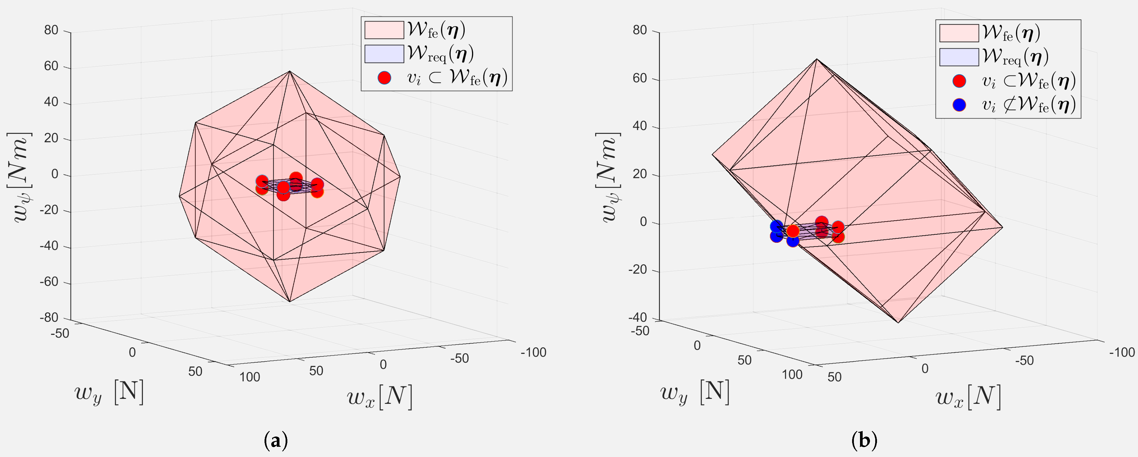
2.3. Wrench Feasible Workspace

In ReaTHM testing, it is crucial to ensure that the cabled actuators can apply the reference load vector onto the physical substructure throughout the testing campaign. to this end, we adopt the notion of wrench feasibility [38,39,40] to specify the workspace where this can be guaranteed (in the CDPR litterature, the term wrench is commonly used to denote the load vector w ):
Definition 1 (Definitions of Wrench Feasibility and Workspaces).
Let the set of feasible wrenches W fe ( η ) = { w R m : w = W ( η ) f ,   f m i n f f m a x } be the set of loads that is feasible at a given pose η. Furthermore, let the wrench feasibility requirement W req ( η ) be the set of all loads that, per requirements, should be feasible at a given pose η. A pose η is said to be wrench feasible if W req ( η ) W fe ( η ) . Let the wrench feasible workspace be the set of poses that are wrench feasible, i.e., N = { η R m : W req ( η ) W fe ( η ) } . Finally, let the wrench feasible workspace requirement N req be the set of poses in which wrench feasibility is required. We say that the CDPR fulfils wrench feasibility requirements if N req N .
Several authors addressed wrench feasibility analytically by constructing geometric bounds of N . See, for example [39]. Although continuous expressions for N can be found for simple geometries, and promising approaches using interval-analysis exist [40], discretisation and subsequent exhaustive numerical evaluation remain popular in the relevant literature due to the complexity of alternative approaches. See the discussion in ([10] [Ch 5]).
In this paper, wrench feasibility is checked using the following proposition:
Proposition 1.
(Adapted from [41].) If W req ( η ) is enclosed by the polyhedron formed by I vertices v i R m with v i W fe ( η ) for i = { 1 , 2 , , I } , then W req ( η ) W fe ( η ) .
This follows simply from the total feasible workspace W fe ( η ) being a convex hull [41] (specifically, it is a zonotope [42]). Due to its simplicity, we suggest using pose dependent box constraints,
W req ( η ) = { w R m : w m i n ( η ) w w m a x ( η ) } ,
where w m i n ( η ) and w m a x ( η ) are the required minimum and maximum load vector constraints for each controlled DOF. Using Proposition 1, with box constraints, there are 2 m vertices to check for each platform (the use of Proposition 1 is later exemplified in Section 4).
An alternative framework for checking of wrench feasibility of a platform configuration, in which the set of feasible loads are described as a linear inequality system is presented in [42,43].

2.4. Cable Collision

To ensure that the platform can move freely within N req , the cables should not collide with each other or with the platform during operation [44]. This is especially relevant if cables cross each other as in [8]. Some sources determine collision-free workspaces using analytical approaches [45]. Since this quickly becomes complex, we suggest assessing cable collisions numerically for each pose using Algorithm 1.
In brief, this algorithm considers the distance between line segments in the workspace. in this process, if needed, the platform shapes can be transformed into a simpler convex shape enclosing the platform hull [46]. Let there be n k straight platform line segments enclosing the platform hull and n straight cable line segments. Then, there are a total of (n−1)! cable to cable line segments and n × n k cable to platform line segments that the algorithm needs to check for collision. Finding the shortest distance between two line segments is a simple well-known mathematical problem with relatively low computational cost. See for example [47].
Algorithm 1Cable Collision.
   δ l i m Critical collision distance.
  for each pose in the grid do
    for each cable, find minimum distances {d} to all other line segments.
    if ( a n y ( { d } ) < δ l i m ) then define as collision (or refine search).
    end if
  end for

2.5. Configuration Performance Measure

As described generally for CDPR setups in ([10] [Ch 8]) and discussed in the paper introduction, each platform configuration can be associated with a performance measure c p ( η ) . A global performance measure k ¯ is obtained by integrating the cost over the entire volume of interest V ( N req ) using
k ¯ = 1 V ( N req ) N req c p ( η ) d N req 1 K i = 1 K c p ( η i ) ,
where the latter is the corresponding approximation summing over N req , which is discretised into K cells.

3. Procedure for Optimal Actuator Placement in ReaTHM Testing

3.1. Performance Measure

In this paper and for use in ReaTHM testing applications we propose using the following platform configuration performance measure given n actuators and a fixed cost function g ( f ) :
c p ( η ) = κ g ( g ( f * ) g ( f 0 ) ) c p g + i = 1 i = m κ 1 [ i ] w ref [ i ] ( f * ) 1 c p 1 + i = 1 i = m κ 2 [ i ] η [ i ] ( f * ) 1 c p 2 + i = 1 i = m κ 3 [ i ] η [ i ] ( W ) f * 1 c p 3
where κ g R 0 1 ,   κ 1 R 0 m ,   κ 2 R 0 m ,   and   κ 3 R 0 m are constant scaling parameters that determine the relative weighting of each term. Further κ ( · ) [ i ] ,   w ref [ i ] and η [ i ] are the i th components of κ ( · ) , w ref , and η , respectively (for example η [ 1 ] denotes x). The notation ∇ denotes partial derivatives. For example, η [ i ] ( f * ) denotes the partial derivative of ( f * ) with respect to the variable η [ i ] . The terms of (8) are expressed mathematically in Appendix A. Finally, f * is the solution f * to (4) given w r e f = 0 . The latter means that the performance for each pose is only evaluated around the static equilibrium point ( w = 0 ) and is a choice made to limit computation times (we expect the performance near w = 0 to be the most important).
Although not done in this work, if computation times are of no concern, it is straightforward to extend (8) such that it for a given pose sums over a weighted version of the wrench feasibility requirement. Another straightforward extension would be multiplying c p ( η ) with a pose-dependent weight. The latter would allow increasing the prioritisation of performance in poses that are particularly important.
The reasoning for each component of (8) is as follows:
  • c p g 
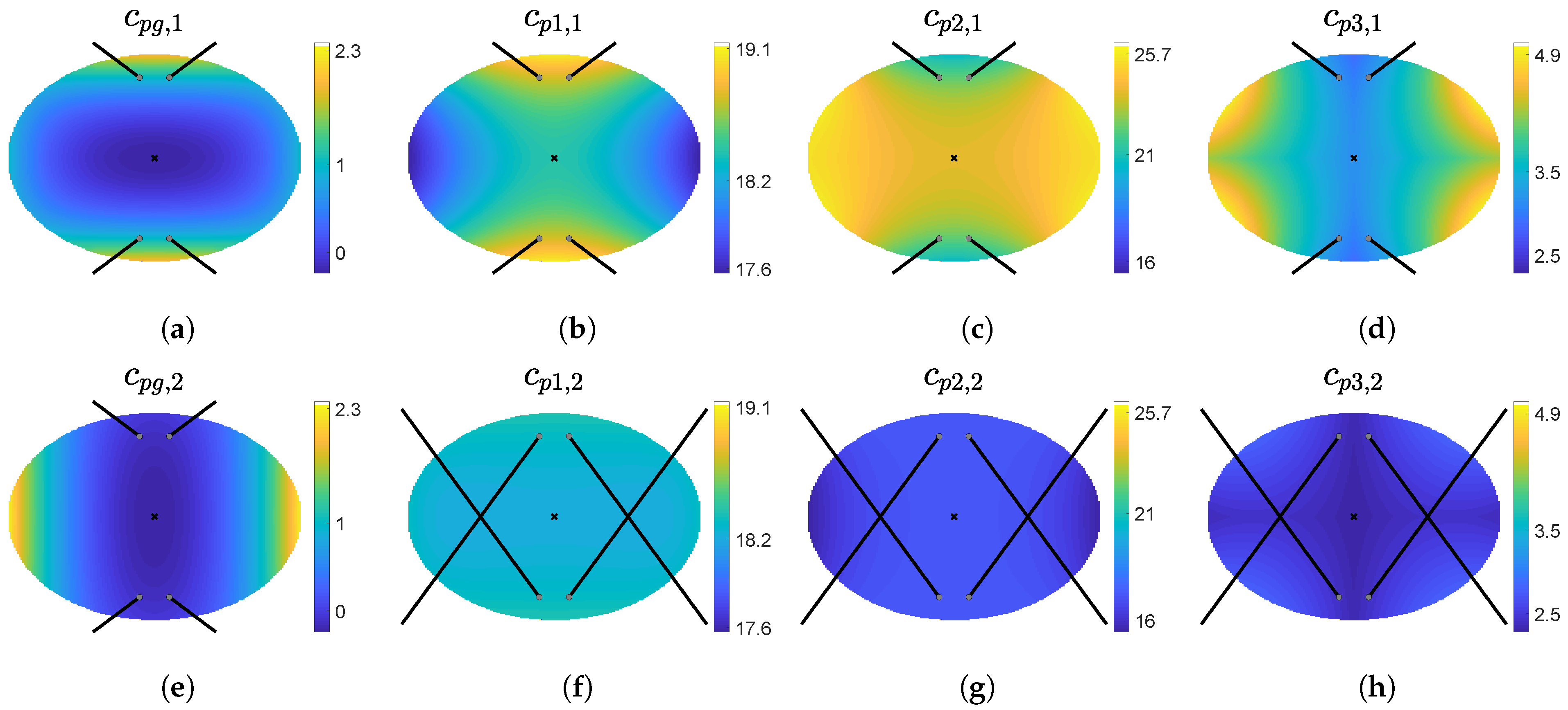
—(quality of tension distribution) associates the cable tensions with the cost captured by the cost function. The cost function is assumed to be designed such that the actuated cables operate at higher performance when g ( f * ) is low.
  • c p 1 —(load vector sensitivity) is a measure of the sensitivity of the optimal cable tensions to a change in the reference load vector. Since f * is the minimiser of the optimisation problem, the term can also be interpreted as a controllability measure that takes the cost function and constraints into account—as opposed to simpler controllability measures based on eigenvectors [22].
  • c p 2 —(motion sensitivity) is a measure of the optimal cable tensions sensitivity to platform motions. The intent is to limit the sensitivity of the optimal cable tensions to motions – to generate smoother trajectories that are easier to track.
  • c p 3 —(kinematic mapping sensitivity) quantifies the actual load vector’s sensitivity to changes in η , given fixed cable tensions f * . Keeping c p 3 low reduces force allocation errors by making the load vector less sensitive to small errors in the pose estimates η ^ . See discussion on force allocation errors in [8]. The term also reduces the stiffness in the weighted degrees of freedom (specifically it reduces stiffness induced from internal forces, which is one of two components of the overall stiffness of a CDPR mechanism [48]).

3.2. Procedure Description

Using the performance measure (8), we formulate the following procedure:
Procedure 1.
Optimal actuator placement for ReaTHM testing using CDPR.
  • (Problem specification) Specify the number of actuators n, the cable cost function g ( f ) , the cable tension constraints f min and f max , the workspace requirements N req   and   W req , the performance measure weights κ g ,   κ 1 ,   κ 2 ,   and   κ 3 , and the constraints in the placement of actuators.
  • (Determination of optimal actuator placement) Given the above specifications, with k ¯ and c ( η ) given by and (7) and (8), respectively, then determine the optimal actuator placement that minimises k ¯ subject to: 1) N req N , 2) no cable collisions, and 3) constraints in the placement of actuators.
By using a performance measure that is a linear combination of terms that all target accurate actuation of forces (that is, quality of force distribution, load vector sensitivity, motion sensitivity, and kinematic mapping sensitivity), Procedure 1 is designed to: (1) increase load tracking accuracy and (2) ensure that the expected numerical loads are always feasible. As such, it is suitable for ReaTHM testing, where load inaccuracies may jeopardize fidelity. Conversely, traditional optimality measures for CDPR applications such as maximising workspaces or minimising the effect of external forces on the platform (by increasing stiffness) are not part of the cost function. This reflects the different prioritisation when considering ReaTHM testing compared to other typical CDPR applications, as discussed in the paper introduction.

3.3. General Guidelines for Problem Specification in Procedure 1

3.3.1. Controlled Degrees of Freedom and the Number of Actuators

Although a higher number of actuators can increase actuation capabilities and the extent of N , each actuator increases the setup’s complexity and is associated with acquisition, installation, and maintenance costs. In the literature on CDPR, it appears to be most common to have either one (for planar CDPR) or two (for 6-DOF CDPR) more actuators than controlled DOFs [49].
For ReaTHM testing, there may be several reasons to have fewer than six controlled DOFs (e.g., m < 6 ). Uncontrolled DOFs are characterized by being self-stabilizing, with the corresponding numerical load component having a negligible impact on the quantities of interest compared to hydrostatic and hydrodynamic loads. See the following examples:
  • In ReaTHM testing of a floating offshore wind turbine reported in [3,7,50], leaving out the vertical component of w r e f is shown to have negligible effect on the motions of the wind turbine, mooring force and internal loads. The physical platform is actuated in five DOFs ( m = 5 ), using six cabled actuators ( n = 6 ).
  • In ReaTHM testing of a moored buoy reported in [51] it is argued that out-of-plane numerical load components can be neglected. Due to the circular, symmetrical shape of the buoy, the yaw moment is also neglected. The physical platform is actuated in two DOFs ( m = 2 ), using three cabled actuators ( n = 3 ).
  • Similarly, for the ReaTHM testing of the ship-shaped vessel reported in [8], out-of-plane numerical load components are neglected (see also [5]). Unlike [51], however, the yaw moment is considered important. The physical platform is actuated in three DOFs ( m = 3 ), using four cabled actuators ( n = 4 ).

3.3.2. Actuator Tension Constraints and Cost function

The actuator cable tension constraints are highly dependent on the characteristics of the actuators in use. A minimum admissible tension f min = ( f min , 1 , f min , 2 , , f min , n ) is set to prevent the cable from going slack, whereas a maximum admissible tension f max = ( f max , 1 , f max , 2 , , f max , n ) is set due to actuator and cable limitations.
Although Procedure 1 is not restricted to a specific cost function, as stated earlier, we propose to reuse the cost function presented in (5). See [36], for guidelines on determining its parameters.

3.3.3. Workspace Requirements

For ReaTHM testing, we recommend adjusting W req and N req based on the expected outputs of the numerical substructure and based on the expected excursions/motions of the model in the basin. These can either be derived from simulation studies or determined heuristically based on simplified analysis, experience, intuitive understanding, and case assessment. If the plan is to reuse the setup in several different testing campaigns, this should be reflected in N req and W req .

3.3.4. Constraints in Placement of Actuators

The actuators will typically be mounted onto existing basin infrastructure (such as along the basin walls), which imposes natural constraints on the placement of the actuators. Other important factors include ease of access for installation and maintenance, including cabling for communication, power, and control.
Enforcing symmetry constraints on the placement of actuators simplifies the design process and increases robustness by alleviating some biases. A symmetric design also conforms to standards for typical CDPR applications. See for example ([10,12,17,21] (Ch 2.3)).

3.3.5. Performance Weights

We suggest the following approach to determine the weights κ g ,   κ 1 ,   κ 2 ,   and   κ 3 :
  • Since κ 1 and κ 2 both relate to target force tracking, they are scaled relative to each other and in proportion to the expected variation in η and w ref –under the assumption that it is easier to track target forces that vary less.
  • Next κ 3 is determined by considering the importance of force allocation errors relative to force tracking errors. If the expected accuracy of η ^ is high, κ 3 can be reduced relative to κ 1 and κ 2 , and increased in the opposite case.
  • Next, the entries of κ 1 ,   κ 2 ,   and   κ 3 are determined in proportion to the expected dynamic range and the variations of η and w r e f . For example, an expectation of large variations in η [ 1 ] , corresponds to an increase in κ 2 [ 1 ] and κ 3 [ 1 ] , as these scaling parameters capture sensitivity to changes in η [ 1 ] . Conversely, an expectation of large variations of w ref [ 1 ] corresponds to an increase in κ 1 [ 1 ] , since this scaling parameter captures sensitivity to w ref [ 1 ] .
  • Finally, the cost vector gain κ g is chosen according to the importance of having a low cost function value relative to keeping the other terms low. This gain will be highly dependent on the selected cost function.

4. Optimal Placement of Actuators for ReaTHM Testing of a Barge

This section demonstrates Procedure 1 by applying it to an example test case closely resembling that of Figure 3, studied by the authors in [8]. Specifically, it considers a case where a moored barge is to be tested in a small basin facility with dimensions 16.2 m × 6.7 m with its side against the incident waves as illustrated in Figure 7. The body-fixed cable lever arms { r i b } are specified in Table 2 (a). Procedure 1 is used to determine the actuator placement { p a } along the basin wall.

4.1. Problem Specification

4.1.1. Controlled Degrees of Freedom and the Number Of Actuators

The numerical substructure is composed of a horizontal model of the barge’s mooring system, with only planar load components transmitted across the partitioning interface, i.e., out-of-plane loads of the mooring system are neglected. This implies that the numerically calculated load vector is to be actuated in the three degrees of freedom surge, sway, and yaw ( x , y , ψ ) . Accordingly, we specify the case with η 3 : = ( x , y , ψ ) in place of η , w : = ( w x , w y , w ψ ) , and m = 3 .
To not use more actuators than necessary, the case is specified with four actuators ( n = 4 ) which is sufficient to ensure that the system is overconstrained.

4.1.2. Constraints in Placement of Actuators

The case is specified with the following constraints on the actuator placement along the basin walls:
  • Each actuator protrudes 10 cm out from the basin wall.
  • The actuators shall be symmetrically placed along the basin walls.
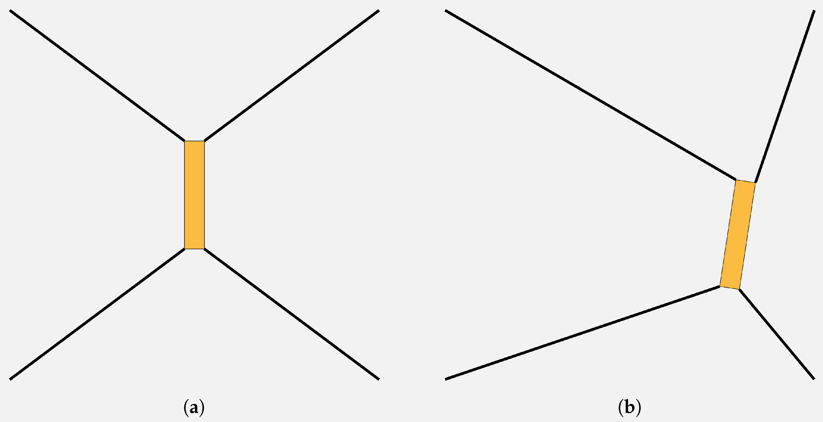
  • Cable 1 may cross Cable 2, and Cable 3 may cross Cable 4 (as in [8]). In case of cable crossing, the cables are raised or lowered by 2.5 centimetres to avoid cable collision. It is assumed that the effect that the introduced z-component of the force has on the emulated system is negligible compared to hydrostatic and hydrodynamic loads.
Mathematically, the four cable exit points ( p a 1 ,   p a 2 ,   p a 3 ,   and   p a 4 ) are constrained by:
p a 1 = x a c t y a c t z c ,   p a 2 = x a c t y a c t z c ,
p a 3 = x a c t y a c t z c ,   p a 4 = x a c t y a c t z c ,
with,
( x a c t , y a c t ) i = 1 3 Λ i ,
where
Λ 1 = { ( x , 3.25 ) | 0 x 8 } ,   Λ 2 = { ( 8 , y ) | 3.25 y 3.25 } ,   Λ 3 = { ( x , 3.25 ) | 0 x 8 }
and
z c = 0.025 ,   if   y a c t 0 0 ,   if   y a c t > 0 .
With the given constraints and symmetry considerations, there is effectively only one optimisation variable, which denotes distance along the three walls ( Λ 1 , Λ 2 , Λ 3 ), parameterised by the variable l p a :
l p a = x a c t ,   if   y a c t = 3.25 ( Λ 1 ) 11.25 y a c t ,   if   x a c t = 8   ( Λ 2 ) 22.5 x a c t ,   if   y a c t = 3.25   ( Λ 3 )
See also Figure 8, which outlines l p a along the basin wall for Actuator 1.

4.1.3. Wrench Feasibility and Workspace Requirements

The intended use of the setup is system identification and estimation of responses to nonlinear wave loads, similar to [5]. Among the important tests for this purpose are decay tests [8], where the vessel is released from an initial offset from the mooring line equilibrium point, as shown in Figure 7. Most of the excitations are expected to be directed along the incident waves coming from the negative x-direction. Also expecting some variations in heading, the workspace requirement is specified as:
N req : = x 2 + 2 y 2 < 3 ( N req , xy ) 20 + 10 x 2 + 2 y 2 3 π 180 ψ 20 10 x 2 + 2 y 2 3 π 180         ,
where N req , xy specify the workspace requirement in the x-y plane with (x,y, ψ ) having units [ m , m , rad ]
The numerically calculated load vector emulates mooring forces that are expected to restore toward the mooring equilibrium ( x ,   y ,   ψ ) = 0 . Taking this into account, incorporating some load vector flexibility and expecting larger loads in x-direction, the wrench feasibility requirement is specified by the following box constraints:
W req ( η 3 )   : = 12 2 x 8 y 2 ψ w + 12 2 x + 8 y 2 ψ ,
where w has units [N,N,Nm].
To verify N req N , Proposition 1 is applied to each cell in the discretised workspace. See Figure 9 and Figure 10 that demonstrate the proposition for the two platform configurations of Table 2. Figure 11 outlines N for the two actuator configurations of Table 2. While both cases satisfy N req N , the cross configuration has a significantly larger wrench feasible workspace.

4.1.4. Cost Function

The designated actuators are similar to those we described in [32], and are specified with the minimum and maximum admission tensions 1 [ N ] and 50 [ N ] , respectively.
For the cost function, we reuse (5) configured with the following parameters:
c 1 = 0.1 , c 2 = 0.1 , α i = 20   f m i n , i = 1 , f m a x , i = 50 , f 0 , i = 10 for   i = 1 , 2 , n .
Example 1.
Wrench feasibility for two sample poses.
In this example Proposition 1 is applied to the two platform configurations of Table 2, given (15). In Platform configuration 1, W fe ( η 3 ) encloses all vertices (red dots), such that W req ( η 3 ) W fe ( η 3 ) , and the pose is wrench feasible. In Platform configuration 2, three vertices (blue dots) are not enclosed by W fe ( η 3 ) such that the platform configuration is not wrench feasible. See Figure 10.
Figure 9. The platform configurations of Table 2. (a) Platform configuration 1 (b) Platform configuration 2.
Jmse 09 00191 g009
Figure 10. Box load vector requirement W req (blue cuboid), relative to feasible loads W fe (red polyhedron), given (15) for the platform configuration of Table 2. W fe is found by the method described in [42] and computed for illustrative purpose only. (a) Platform configuration 1. (b) Platform configuration 2.
Jmse 09 00191 g010

4.1.5. Performance Measure Weights

The following performance measure weights are chosen:
κ g = 10 , κ 1 = 5 κ x κ y 0.5 κ 2 = 1 κ x κ y 0.1 κ 3 = 0.2 κ x κ y 0.1 .
These are determined as follows: (1) over the testing campaign, we expect the numerical variations in w ref , to be about five times larger than η 3 (this is also reflected in (14) and (15)), and put a five times larger gain for κ 1 than that of κ 2 . (2) Based on experimental experience, we expect that the accuracy of the estimates η ^ 3 is high and that force tracking errors are more critical to performance than errors in η ^ 3 . We therefore scale κ 3 with a lower gain of 0.2. (3) Since ψ ˙ [rad/s] is expected to be significantly smaller in magnitude than ( x ˙ , y ˙ ) [m/s], the gains associated with changes in ψ are scaled with a gain of 0.1 (applies to κ 2   and   κ 3 ). For similar reasons, we scale moments with gain of 0.5 relative to translational forces (applies to κ 1 ). We leave κ ( · ) [ 1 ] and κ ( · ) [ 2 ] as priority parameters κ x and κ y . (4) Considering that the cost function value is typically low (due to division by α 2 ), we set κ g = 10 , which ensures that the term has a moderately smaller impact on the global performance measure function than the other terms.
Figure 11. Visual representation of the wrench feasible workspace N for the two actuator configurations of Table 2. The black lines represent cables configuration at η 3 = 0 . The colour is a measure of wrench feasibility as a function of ψ (in degrees). For example, if the colour of a cell indicates a value of 20, it is wrench feasible with 20 < ψ < 20   [ deg ] . (a) Actuator configuration 1 (uncrossed). (b) Actuator configuration 2 (crossed).
Jmse 09 00191 g011
For more insight, and to further support the choice of κ values, Table 3 presents the terms of (8) for the two platform configurations of Table 2 and Figure 12 shows the resulting cost terms of (8) over N req , xy for the two actuator configurations of Table 2. Table 3 demonstrates how the terms of (8) are significantly more sensitive to rotational than translational motions—as also reflected in the chosen weights. Also, since Platform configuration 2 is farther from the centre of the workspace, it is associated with more variation in cable tensions and less controllability—resulting in significantly higher costs than in Platform configuration 1. Figure 12 shows how the cost increases toward the edges of the workspace and how the crossed configuration is associated with significantly lower costs than the uncrossed configuration. When considering Figure 12, it should be noted that constant common offsets have no effect on the optimisation procedure. Instead, the variations of each term between different platform configurations should be considered.

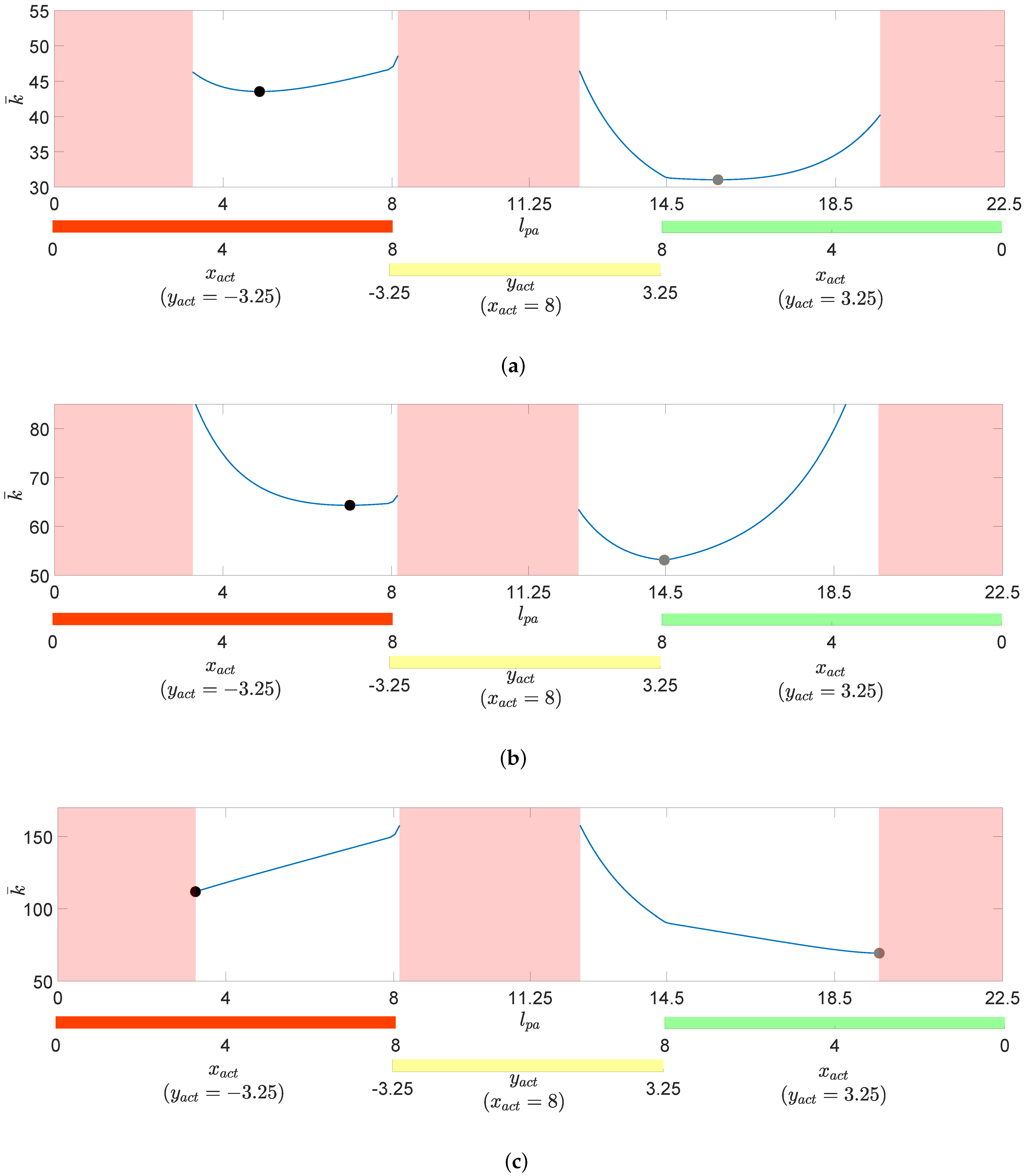
4.2. Determination of Optimal Actuator Placement

In this section, the actuator placement is determined for the given case, i.e., Procedure 1 is used with the actuator constraints given by (9)–(13), the cable cost function given by (5), the wrench feasible workspace requirements given by (14) and (15), and the performance measure weights given by (17).
The procedure is considered for three different sets of κ x   and   κ y : Prioritisation 1) κ x = 1   and   κ y = 1 , Prioritisation 2) κ x = 4   and   κ y = 1 , and Prioritisation 3) κ x = 1   and   κ y = 4 . Whereas Prioritisation 1 represents a base case with equal weighting in x and y direction, Prioritisation 2 is in line with the considered test case that expects most movement and loads to be directed in x-direction. Finally, Prioritisation 3, where the weight in y-direction is the highest, is included for comparison reasons.
Figure 13 shows the resulting global performance measure k ¯ as a function of l p a for each of the three cases. The optimal placement is indicated in the figure both with uncrossed cable configuration (black mark) and with crossing cables (grey mark). The corresponding actuator placements are detailed in Table 4 and shown geometrically in Figure 14.
We note that for all three cases, the crossed configuration yields significantly lower cost κ ¯ – and thus represent a higher performing actuator configuration. Given the smaller basin dimensions of the test case, this can be explained by the cross-configuration enabling longer cable lengths and higher controllability. Crossed cable configuration yielding better performance is in line with previous work. See for example ([10] [Ch 8]). It also conforms with the author’s experiences with earlier testing campaigns on the experimental setup shown in Figure 3.
While there are multiple trade-offs, captured by the global performance measure, we observe that the procedure tends to account for the change of prioritisation by aligning the cable attack angles in the direction of the higher weighted DOF. For Prioritisation 2, which corresponds to the considered test case, the actuators are placed quite far in x-direction from the origin (see Figure 14b), which should allow high performance for the specified case, where most of the expected movements and loads are in the x-direction.

4.3. A Delimiting Note

As discussed at a general level for CDPR setups in ([10] [Ch 8]), platform configuration performance measures are typically not complete in the sense that there is usually some ambiguity and uncertainty in the choice of performance measure design parameters. Moreover, it can be challenging to prove that the actuator placement that minimises the cost function corresponds to a practically optimal CDPR design. These considerations also apply for Procedure 1. As such, the proposed procedure should be considered to be a tool that aids the laboratory-engineer in determining actuator placement.

5. Conclusions

In this paper, we presented a procedure for placement of actuators on CDPR setups, particularly suitable for ReaTHM testing. The procedure incorporates performance measures that maximise load tracking accuracy, while ensuring that the numerically calculated loads are always applicable according to specified workspace requirements. In this sense, the present work contributes to robust and well-performing actuator placement in ReaTHM testing, for which no other such guidelines exist.
Future work on the method includes application to more complex cases, in-depth analysis of the impact that each term of (8) has on load tracking accuracy, and refinement of the guidelines for selecting the performance measure weights.

Author Contributions

Conceptualization, E.U.; methodology, E.U.; software, E.U.; validation, E.U., T.S. and R.S.; formal analysis, E.U.; investigation, E.U., T.S. and R.S.; writing—original draft preparation, E.U.; writing–review and editing, E.U., T.S., and R.S.; visualization, E.U.; supervision, T.S. and R.S.; project administration, R.S.; funding acquisition, R.S and T.S. All authors have read and agreed to the published version of the manuscript.

Funding

This work was supported by grant No. 254845 ReaTHM testing for Extreme Marine Environments and the Research Council of Norway through the Centre of Excellence NTNU AMOS, project no. 223254.

Institutional Review Board Statement

Not applicable.

Informed Consent Statement

Not applicable.

Data Availability Statement

Not applicable.

Conflicts of Interest

The authors declare no conflict of interest.

Abbreviations

The following abbreviations are used in this manuscript:
CDPRCable-driven parallel robot
ReaTHM testing * Real-time hybrid model testing
DOFDegrees of freedom
* ReaTHM® testing is a registered trademark of SINTEF Ocean.

Appendix A. Expression for the Terms of (8)

This section writes out the terms of (8). For conciseness, the ∇ notation denotes partial derivatives. For example η [ i ] W ( η ) denotes d W ( η ) d η [ i ] .
As elaborated in [36], given some necessary assumptions, at the solution to (8), the following conditions are satisfied.
C ( z ) = f g ( f * ) + W λ W f * w ref = 0 ,   where   z = f * , λ .
The underlying solver described in [36] finds z using Newtons iterations. Once z is found, it is numerically cheap to find the terms of (8) as outlined next.
The partial derivative of z with respect a parameter p is
z p = C z 1 C p = H 1 C p , where   H = f 2 g ( f ) W W 0 .
Furthermore, the partial derivatives of R with respect to w ref [ i ] and η [ i ] is
C w ref [ i ] = 0 R n × 1 d i R m × 1 , C η [ i ] = η [ i ] W ( η ) λ η [ i ] W ( η ) f * ,
where d i R m is a vector that has all zero-entries except the ith entry which equals -1 and
η [ i ] W ( η ) = η [ i ] j 1 η [ i ] j 2 η [ i ] j n ,   with   η [ i ] j i = η [ i ] u i r i a × η [ i ] u i + η [ i ] r i a × u i .
The components of (A4), written out for each i in η [ i ] are
x r i a = 0 , y r i a = 0 , z r i a = 0 , θ r i a = R z ( ψ ) R y ( ϕ ) R x ( θ ) S x r i b
ϕ r i a = R z ( ψ ) R y ( ϕ ) S y R x ( θ ) r i b , ψ r i a = R z ( ψ ) S z R y ( ϕ ) R x ( θ ) r i b
x u i = 1 / l c , i 3 ( Δ y 2 Δ z 2 ) ( Δ x Δ y ) ( Δ x Δ z )
y u i = 1 / l c , i 3 ( Δ x Δ y ) ( Δ x 2 Δ z 2 ) ( Δ y Δ z )
z u i = 1 / l c , i 3 ( Δ x Δ z ) ( Δ y Δ z ) ( Δ x 2 Δ y 2 )
θ u i = x u i y u i z u i θ ( r )
ϕ u i = x u i y u i z u i ϕ ( r )
ψ u i = x u i y u i z u i ψ ( r ) ,
where S x = 0 0 0 0 0 1 0 1 0 , S y = 0 0 1 0 0 0 1 0 0 , S z = 0 1 0 1 0 0 0 0 0 ,
Δ x Δ y Δ z T = ( p a i p e i ) , and l c , i = | p a i p e i | 2 .
The first term of (8) is given directly by the cost function, whereas inserting (A3) into (A2) and substituting p with w r e f [ i ] and η [ i ] gives the second and third term of (8), respectively. Finally, the last term of (8) is found using (A4) directly.
As (A5)(a–h) indicates, larger basins and cable distances, tend to reduce the cost c p . This is especially the case for c p 2 and c p 3 , as evident by the factor 1 / l c , i 3 in (A5)(a–h). In cases where longer cable length is expected to have detrimental effects, this can be accounted by in the cost function.

References

  1. Sauder, T. Fidelity of Cyber-Physical Empirical Methods: A Control System Perspective. In Experimental Techniques; Springer: Berlin/Heidelberg, Germany, 2020; pp. 1–17. [Google Scholar]
  2. Chabaud, V. Real-Time Hybrid Model Testing of Floating Wind Turbines. Ph.D. Thesis, Norwegian University of Science and Technology, Trondheim, Norway, 2016. [Google Scholar]
  3. Sauder, T.; Chabaud, V.; Thys, M.; Bachynski, E.E.; Sæther, L.O. Real-time hybrid model testing of a braceless semi-submersible wind turbine: Part I—The hybrid approach. In Proceedings of the ASME 2016 35th International Conference on Ocean, Offshore and Arctic Engineering. American Society of Mechanical Engineers Digital Collection, Busan, Korea, 19–24 June 2016. [Google Scholar]
  4. Chakrabarti, S. Physical model testing of floating offshore structures. In Proceedings of the Dynamic Positioning Conference, Citeseer, HO, USA, 13–14 October 1998. [Google Scholar]
  5. Sauder, T.; Tahchiev, G. From soft mooring to active positioning in laboratory experiments. In Proceedings of the 39th International Conference on Ocean, Offshore and Arctic Engineering. American Society of Mechanical Engineers Digital Collection, Virtual, Online, 3–7 August 2020. [Google Scholar]
  6. Vilsen, S.A.; Sauder, T.; Sørensen, A.J.; Føre, M. Method for Real-Time Hybrid Model Testing of ocean structures: Case study on horizontal mooring systems. Ocean. Eng. 2019, 172, 46–58. [Google Scholar] [CrossRef]
  7. Chabaud, V.B.; Eliassen, L.; Thys, M.; Sauder, T.M. Multiple-degree-of-freedom actuation of rotor loads in model testing of floating wind turbines using cable-driven parallel robots. J. Phys. Conf. Ser. 2018, 1104, 012021. [Google Scholar] [CrossRef]
  8. Ueland, E.S.; Skjetne, R.; Vilsen, S.A. Force Actuated Real-Time Hybrid Model Testing of a Moored Vessel: A Case Study Investigating Force Errors. FAC-PapersOnLine 2018, 51, 74–79. [Google Scholar] [CrossRef]
  9. Gosselin, C.; Grenier, M. On the determination of the force distribution in overconstrained cable-driven parallel mechanisms. Meccanica 2011, 46, 3–15. [Google Scholar] [CrossRef]
  10. Pott, A. Cable-Driven Parallel Robots: Theory and Application; Springer: Berlin/Heidelberg, Germany, 2018. [Google Scholar]
  11. Rodnunsky, J.; Bayliss, T. Aerial Cableway and Method for Filming Subjects in Motion. U.S. Patent 5,224,426, 6 July 1993. [Google Scholar]
  12. Pott, A.; Mütherich, H.; Kraus, W.; Schmidt, V.; Miermeister, P.; Verl, A. IPAnema: A family of cable-driven parallel robots for industrial applications. In Cable-Driven Parallel Robots; Springer: Berlin/Heidelberg, Germany, 2013. [Google Scholar]
  13. Newman, M.; Zygielbaum, A.; Terry, B. Static analysis and dimensional optimization of a cable-driven parallel robot. In Cable-Driven Parallel Robots; Springer: Berlin/Heidelberg, Germany, 2018. [Google Scholar]
  14. Horoub, M.; Hawwa, M. Influence of cables layout on the dynamic workspace of a six-DOF parallel marine manipulator. Mech. Mach. Theory 2018, 129, 191–201. [Google Scholar] [CrossRef]
  15. Kraus, W.; Schmidt, V.; Rajendra, P.; Pott, A. System identification and cable force control for a cable-driven parallel robot with industrial servo drives. In Proceedings of the 2014 IEEE International Conference on Robotics and Automation (ICRA), Hong Kong, China, 31 May–7 June 2014. [Google Scholar]
  16. Oh, S.R.; Agrawal, S.K. Cable suspended planar robots with redundant cables: Controllers with positive tensions. IEEE Trans. Robot. 2005, 21, 457–465. [Google Scholar]
  17. Lamaury, J.; Gouttefarde, M. A tension distribution method with improved computational efficiency. In CDPRs; Springer: Berlin/Heidelberg, Germany, 2013. [Google Scholar]
  18. Rushton, M.; Khajepour, A. Optimal actuator placement for vibration control of a planar cable-driven robotic manipulator. In Proceedings of the 2016 American Control Conference (ACC), Boston, MA, USA, 6–8 July 2016. [Google Scholar]
  19. Kim, Y.; Junkins, J.L. Measure of controllability for actuator placement. J. Guid. Control. Dyn. 1991, 14, 895–902. [Google Scholar] [CrossRef]
  20. Pusey, J.; Fattah, A.; Agrawal, S.; Messina, E. Design and workspace analysis of a 6–6 cable-suspended parallel robot. Mech. Mach. Theory 2004, 39, 761–778. [Google Scholar] [CrossRef]
  21. Aref, M.M.; Taghirad, H.D.; Barissi, S. Optimal design of dexterous cable driven parallel manipulators. Int. J. Robot. 2009, 1, 29–47. [Google Scholar]
  22. Abdolshah, S.; Zanotto, D.; Rosati, G.; Agrawal, S.K. Optimizing stiffness and dexterity of planar adaptive cable-driven parallel robots. J. Mech. Robot. 2017, 9, 031004. [Google Scholar] [CrossRef]
  23. Anson, M.; Alamdari, A.; Krovi, V. Orientation workspace and stiffness optimization of cable-driven parallel manipulators with base mobility. J. Mech. Robot. 2017, 9, 031011. [Google Scholar] [CrossRef]
  24. Jamshidifar, H.; Khajepour, A.; Fidan, B.; Rushton, M. Kinematically-constrained redundant cable-driven parallel robots: Modeling, redundancy analysis, and stiffness optimization. IEEE/ASME Trans. Mechatron. 2016, 22, 921–930. [Google Scholar] [CrossRef]
  25. Ouyang, B.; Shang, W. Wrench-feasible workspace based optimization of the fixed and moving platforms for cable-driven parallel manipulators. Robot. Comput. Integr. Manuf. 2014, 30, 629–635. [Google Scholar] [CrossRef]
  26. Song, D.; Zhang, L.; Xue, F. Configuration optimization and a tension distribution algorithm for cable-driven parallel robots. IEEE Access 2018, 6, 33928–33940. [Google Scholar] [CrossRef]
  27. Azizian, K.; Cardou, P. The dimensional synthesis of planar parallel cable-driven mechanisms through convex relaxations. J. Mech. Robot. 2012, 4, 031011. [Google Scholar] [CrossRef]
  28. Bryson, J.T.; Jin, X.; Agrawal, S.K. Optimal design of cable-driven manipulators using particle swarm optimization. J. Mech. Robot. 2016, 8, 041003. [Google Scholar] [CrossRef] [PubMed]
  29. Gouttefarde, M.; Collard, J.F.; Riehl, N.; Baradat, C. Geometry selection of a redundantly actuated cable-suspended parallel robot. IEEE Trans. Robot. 2015, 31, 501–510. [Google Scholar] [CrossRef] [Green Version]
  30. Sauder, T.; Marelli, S.; Sørensen, A.J. Probabilistic robust design of control systems for high-fidelity cyber-physical testing. Automatica 2019, 101, 111–119. [Google Scholar] [CrossRef] [Green Version]
  31. Sauder, T.; Marelli, S.; Larsen, K.; Sørensen, A.J. Active truncation of slender marine structures: Influence of the control system on fidelity. Appl. Ocean. Res. 2018, 74, 154–169. [Google Scholar] [CrossRef] [Green Version]
  32. Ueland, E.; Sauder, T.; Skjetne, R. Force Tracking Using Actuated Winches with Position Controlled Motors for Use in Hydrodynamic Model Testing. IEEE Access 2021. submitted for publication. [Google Scholar]
  33. Hussein, H.; Santos, J.C.; Gouttefarde, M. Geometric optimization of a large scale CDPR operating on a building facade. In Proceedings of the 2018 IEEE/RSJ International Conference on Intelligent Robots and Systems (IROS), Madrid, Spain, 1–5 October 2018. [Google Scholar]
  34. Robohub/Max Planck Institute for Biological Cybernetics. Cable-Driven Parallel Robots: Motion Simulation in a New Dimension. Available online: https://robohub.org/cable-driven-parallel-robots-motion-simulation-in-a-new-dimension (accessed on 15 May 2020).
  35. Fraunhofer IPA. Cable-Driven Parallel Robots. Available online: https://www.ipa.fraunhofer.de/en/expertise/robot-and-assistive-systems/intralogistics-and-material-flow/cable-driven-parallel-robot.html (accessed on 4 January 2021).
  36. Ueland, E.; Sauder, T.; Skjetne, R. Optimal Force Allocation for Overconstrained Cable-Driven Parallel Robots: Continuously Differentiable Solutions With Assessment of Computational Efficiency. IEEE Trans. Robot. 2020. [Google Scholar] [CrossRef]
  37. Fossen, T.I. Handbook of Marine Craft Hydrodynamics and Motion Control; John Wiley & Sons: Hoboken, NJ, USA, 2011. [Google Scholar]
  38. Ebert-Uphoff, I.; Voglewede, P.A. On the connections between cable-driven robots, parallel manipulators and grasping. In Proceedings of the IEEE International Conference on Robotics and Automation (ICRA ’04), New Orleans, LA, USA, 26 April–1 May 2004. [Google Scholar]
  39. Bosscher, P.M. Disturbance Robustness Measures and Wrench-Feasible Workspace Generation Techniques for Cable-driven Robots. Ph.D. Thesis, Georgia Institute of Technology, Atlanta, GA, USA, 2004. [Google Scholar]
  40. Gouttefarde, M.; Daney, D.; Merlet, J.P. Interval-analysis-based determination of the wrench-feasible workspace of parallel cable-driven robots. IEEE Trans. Robot. 2011, 27, 1–13. [Google Scholar] [CrossRef] [Green Version]
  41. Bosscher, P.; Riechel, A.T.; Ebert-Uphoff, I. Wrench-feasible workspace generation for cable-driven robots. IEEE Trans. Robot. 2006, 22, 890–902. [Google Scholar] [CrossRef]
  42. Bouchard, S.; Gosselin, C.; Moore, B. On the ability of a cable-driven robot to generate a prescribed set of wrenches. J. Mech. Robot. 2010, 2, 011010. [Google Scholar] [CrossRef] [Green Version]
  43. Gouttefarde, M.; Krut, S. Characterization of parallel manipulator available wrench set facets. In Advances in Robot Kinematics: Motion in Man and Machine; Springer: Berlin/Heidelberg, Germany, 2010; pp. 475–482. [Google Scholar]
  44. Lahouar, S.; Ottaviano, E.; Zeghoul, S.; Romdhane, L.; Ceccarelli, M. Collision free path-planning for cable-driven parallel robots. Robot. Auton. Syst. 2009, 57, 1083–1093. [Google Scholar] [CrossRef]
  45. Perreault, S.; Cardou, P.; Gosselin, C.M.; Otis, M.J.D. Geometric determination of the interference-free constant-orientation workspace of parallel cable-driven mechanisms. J. Mech. Robot. 2010, 2, 031016. [Google Scholar] [CrossRef]
  46. Nguyen, D.Q.; Gouttefarde, M. On the improvement of cable collision detection algorithms. In Cable-Driven Parallel Robots; Springer: Berlin/Heidelberg, Germany, 2015. [Google Scholar]
  47. Sunday, D. Distance between 3D Lines and Segments. Available online: https://geomalgorithms.com/a07-_distance.html (accessed on 15 May 2020).
  48. Bolboli, J.; Khosravi, M.A.; Abdollahi, F. Stiffness feasible workspace of cable-driven parallel robots with application to optimal design of a planar cable robot. Robot. Auton. Syst. 2019, 114, 19–28. [Google Scholar] [CrossRef]
  49. Gouttefarde, M.; Lamaury, J.; Reichert, C.; Bruckmann, T. A Versatile Tension Distribution Algorithm for n-DOF Parallel Robots Driven by n+2 Cables. IEEE Trans. Robot. 2015, 31, 1444–1457. [Google Scholar] [CrossRef] [Green Version]
  50. Bachynski, E.E.; Chabaud, V.; Sauder, T. Real-time hybrid model testing of floating wind turbines: Sensitivity to limited actuation. Energy Procedia 2015, 80, 2–12. [Google Scholar] [CrossRef] [Green Version]
  51. Vilsen, S.A.; Sauder, T.; Sørensen, A.J. Real-Time Hybrid Model Testing of Moored Floating Structures Using Nonlinear Finite Element Simulations. In Dynamics of Coupled Structures; Springer: Berlin/Heidelberg, Germany, 2017; Volume 4. [Google Scholar]
1.
What constitutes a typical CDPR application has been inferred based on the trends observed by examining a large number of references. Being trends only, there exist counterexamples for each statement in Table 1.
Figure 1. ReaTHM testing of an ocean structure. ω ( · ) represents environmental loads acting on the structure.
Jmse 09 00191 g001
Figure 2. ReaTHM testing of a moored ship. Notice the four nylon strings used to apply the numerically calculated mooring loads onto the ship. See [6,8].
Jmse 09 00191 g002
Figure 3. ReaTHM testing of a moored barge using a planar CDPR. Red arrows mark the direction of the actuated force, passed axially through each cable. (a,b) Image from laboratory setup of the authors [8]. (a) Crossed configuration. (b) Uncrossed configuration. (c) Schematic overview.
Jmse 09 00191 g003
Figure 4. Two CDPR setups. (a) The CableRobot Simulator [34]. Reproduced with permission from Max Planck Institute for Biological Cybernetics ©2015. (b) The IPAnema 3 CDPR [35]. Reproduced with permission from Fraunhofer IPA © 2019.
Jmse 09 00191 g004
Figure 5. Reference frames and the experimental test setup with the platform (down-scaled physical substructure) connected to n actuated cables. One of the actuators is sketched and annotated.
Jmse 09 00191 g005
Figure 6. The ReaTHM testing loop.
Jmse 09 00191 g006
Figure 7. The moored barge in various poses and with the horizontal required workspace η req ,   xy indicated. Green and yellow colours indicate trajectories in two different test runs.
Jmse 09 00191 g007
Figure 8. Moored barge in the basin, highlighting allowed placement of cable exit point for Cable 1.
Jmse 09 00191 g008
Figure 12. Cost maps for the terms of (8) for the two actuator configurations of Table 2 using (17) with κ x = 1 and κ y = 1 . The black lines represent cables configuration at η 3 = 0 . Coloured area is N req , xy . (ad) Actuator configuration 1. (eh) Actuator configuration 2.
Jmse 09 00191 g012
Figure 13. Performance measure cost function as a function of actuator placement, highlighting minimum for both crossed and uncrossed cable configuration. Cables are in crossed configuration when l p a > 11.25 (a) κ x = 1 , κ y = 1 . (b) κ x = 4 , κ y = 1 . (c) κ x = 1 , κ y = 4 .
Jmse 09 00191 g013
Figure 14. Resulting optimal actuator placement. Black lines are optimal placement with uncrossed cable configuration, and grey lines are optimal placement if crossed configuration is used. (a) κ x = 1 , κ y = 1 . (b) κ x = 4 , κ y = 1 . (c) κ x = 1 , κ y = 4 .
Jmse 09 00191 g014
Table 1. Differences between CDPR in typical applications and CDPR in ReaTHM testing.
Typical CDPR Applications.CDPR for ReaTHM Testing (Using Load Control)
(1) Control objectiveA target pose is the control objective. Force/tension control may be used in an inner control loop to achieve the desired pose. See discussion in [32].A target load vector is the control objective, with pose trajectories following consequently [6].
(2) External forcesThe cabled actuators help ensure that the platform remains close to the desired pose in the presence of external excitations [33].The loads applied by the cabled actuators are in addition to other external loads (typically hydrodynamic) acting on the platform. the applied loads should not be disturbed by the external loads, nor the platform’s movements [8].
(3) Platform weightThe platform is suspended in air, and the platform weight is carried by the cabled actuators. See Figure 4.The platform is located in a water basin, and the cabled actuators do not carry its weight. See Figure 3.
(4) Design considerationsThe CDPR setup is designed for the specific objectives of the application. Typical objectives include to carry a payload or to sense or interact with the environment in a specific way ([10] [Ch 2.4]).The platform is designed to achieve similarity to the target ocean substructure it models (typically using Froude scaling). the objective is for the actuated load vector to track the reference load vector with high accuracy [7].
Table 2. Sample actuator and platform configurations used in Section 4.
(a) { r b } used throughout Section 4.
1234
x0.1750.175−0.175−0.175
y0.95−0.95−0.950.95
z0000
(b) Sample actuator configurations.
{ p a }{ r b }
Actuator configuration 1Table 2 (a)Table 2 (d)
Actuator configuration 2Table 2 (a)Table 2 (e)
(c) Sample platform configurations
Platform configuration 1Actuator configuration 1 with η 3 = ( 0 , 0 , 0 )
Platform configuration 2Actuator configuration 1 with η 3 = ( 1.9 , 0.7 , 0.15 )
(d) { p a } uncrossed configuration(e) { p a } crossed configuration
1234 1234
x3.253.25−3.25−3.25x3.253.25−3.25−3.25
y3.25−3.25−3.253.25y−3.253.253.25−3.25
z0000z−0.0250.025−0.0250.025
Table 3. Terms of (8), for the two platform configurations of Figure 9/Table 2.
w ref [ i ] ( f * ) w ref [ i ] ( f * ) η [ i ] ( W ) f * g ( f * ) g ( f 0 )
Platform configuration 1 0.31 0.42 0.38 0.31 0.42 0.38 0.31 0.42 0.38 0.31 0.42 0.38 1.33 3.18 14.61 1.33 3.18 14.61 1.33 3.18 14.61 1.33 3.18 14.61 4.26 0 0 0 7.62 0 0 0 38.32 −2.3784
Platform configuration 2 1.02 0.39 1.08 0.89 0.6 0.51 0.26 0.36 1.17 0.4 0.1 0.5 5.42 1.44 22.7 3.4 2.38 4.26 1.08 3.91 31.05 3.31 1.68 22.24 7.81 1.2 0.15 1.2 5.29 2.95 0.15 2.95 39.31 −1.9314
Table 4. Test case resulting optimal actuator placement as defined in (9).
Uncrossed ConfigurationCrossed Configuration
( x act , y act )( x act , y act )
Prioritisation 1(4.86, 3.25)(6.78, −3.25)
Prioritisation 2(7.01, 3.25)(8, −3.22)
Prioritisation 3(3.28, 3.25)(2.94, −3.25)
Publisher’s Note: MDPI stays neutral with regard to jurisdictional claims in published maps and institutional affiliations.

