Abstract
In order to improve the accuracy of the freefall of lifeboat motion simulation in a ship life-saving simulation training system, a mathematical model using the strip theory and Kane’s method is established for the freefall of the lifeboat into the water from a ship. With the boat moving on a skid, the model of the ship’s maneuvering mathematical group (MMG) is used to model the motion of the ship in the waves. Based on the formula of elasticity and friction theory, the forces of the skid acting on the boat are calculated. When the boat enters the water, according to the analytical solution theory of slamming, the slamming force of water entry is solved. The simulation experiments are carried out by the established model. The results of the numerical simulation are compared with the calculation results of the hydrodynamics software Star CCM+ at water entry under initial condition A in the paper. The position and velocity of the center of gravity of the boat, the angle, and velocity and acceleration of pitch calculated by the two methods are in good agreement. There is a little difference between the values of translation acceleration calculated by the two methods, which is acceptable. This shows that our numerical algorithm has good accuracy. A qualitative analysis is performed to find the safe point of water entry under the condition of different wave heights and two situations of a ship encountering waves. Finally, the model is applied to the ship life-saving training system. The model can meet the system requirements and improve the accuracy of the simulation.
1. Introduction
1.1. Motivation
The lifeboat is the main life-saving equipment onboard ships. When a shipwreck accident occurs, the crew onboard can quickly escape from the ship by the lifeboat. During the freefall of the lifeboat, the hull of the boat usually slams into the water at high speed, with huge instantaneous impact pressure. If the crews make a mistake when launching the lifeboat, it can cause serious damage to the hull structure and threaten the personal safety of the crew [1]. According to the International Convention on Standards of Training, Certification and Watchkeeping for Seafarers, 1978, as amended in 1995 (STCW 78/95), the crew must be trained and pass a lifeboat assessment before boarding [2]. Training is limited by factors such as time and costs. In recent years, virtual reality technology has developed rapidly, and has been used in training for marine life-saving [3,4]. In order to improve the immersion experience and the reality of the ship’s life-saving training system, a mathematical model is established for the motion of the lifeboat’s freefall during its launch from the ship.
1.2. Related Work
Re et al. [5,6,7] conducted a series of model experiments of a boat launched from a fixed platform. The main focus of the experimental evaluation was the performance of the boat in a range of different weather conditions. Hollyhead et al. [8] and Hwang et al. [9] performed experiments on launching boats from moving ships. They analyzed the motion parameters and the load of the boat. Due to the limitation of experimental conditions, they could only analyze parameters that affected the water entry motion of the boat and did their experiments under good environmental conditions.
In addition to the model experiment, some scholars used a computational method to analyze the freefall of the boat, which was mainly divided into two aspects. First, computational fluid dynamics (CFD) technology was used to numerically simulate the water entry of the lifeboat, and the slamming load of the hull was analyzed by the simulated results [10,11,12]. The second method was to establish a mathematical model for the freefall of the lifeboat for predicting the lifeboat motion attitude, and analyzing the risk of injury to the crew [13,14,15]. The mathematical model of the water entry of the lifeboat’s freefall started from Karman’s momentum theorem, solving the problem of water impact [16]. Boef [17,18] applied Karman’s theory to the modeling of the lifeboat’s motion, and divided the force of the lifeboat entering the water into gravity, buoyancy, drag, and slamming force. Arai et al. [19,20] simplified Boef’s model. They divided the lifeboat’s motion into four stages, sliding phase, rotation phase, freefall phase, and water entry phase, and analyzed the local acceleration of the bow, midship, and stern. The calculation results of local acceleration were close to the model experiment data. Khondoker et al. [21,22,23] applied Arai’s model to analyze the parameters that affect the boat’s water entry. Karim et al. [24,25] applied Arai’s model and took the effect of regular waves into account when calculating speed of the boat entering the water. Raman-Nair and White [26] used multibody dynamics to analyze the entry of the boat from an offshore platform with simple movement. The rotation phase at skid exit is automatically modeled in this way. They regarded the skid as a slope, and the lifeboat as a cube on the slope and as a cylinder at water entry. When calculating the slamming force, they added the item of incident wave force in addition to the item of momentum theory, considering the effect of waves [27,28]. Dymarski and Dymarski [29] studied the model of a lifeboat released into the water from the stern of a ship. They also regarded the skid as a slope and the lifeboat as a cube on the slope, considering the reaction of the boat to the skid, but the motion of the ship was not considered. The detail of the algorithm was not given.
In summary, the current mathematical models for the freefall of the lifeboat do not take motion of ships in waves into account, and the contact force between the boat and skid is not modeled according to their actual structure. The slamming force is calculated according to momentum theory. All algorithms are not compared with real boat experiments or fluid dynamics software.
1.3. Our Contributions
This paper presents a computational model for the simulation of lifeboat freefall during its launching from a ship in rough seas. In order to consider the effect of the ship’s motion on lifeboat motion, the maneuvering mathematical group (MMG) model is used to simulate the motion of the ship in the waves. In order to improve the calculation accuracy, the contact force between boat and skid is calculated based on strip theory, according to the actual structure of the boat and skid. When the boat enters the water, the slamming force is solved based on the theory of energy. The added mass of the boat is calculated according to its size and depth of water entry. Finally, the equations of motion of a freefall lifeboat are formulated using Kane’s method.
A series of simulation experiments are carried out by using the computational model established in this paper. The results of simulation experiments are compared with results of the fluid dynamics software Star CCM+. They show that our numerical algorithm has good accuracy. A qualitative analysis is performed to find a safe point of water entry under the condition of different wave heights and two situations of a ship encountering waves.
Section 2 describes the mathematical model of the motion of boat on the skid. Section 3 describes the mathematical model of boat’s water entry. The setup, results, and analysis of the simulation experiments are presented in Section 4. Section 5 describes an application of the mathematical model and Section 6 gives conclusions.
2. Motion of the Boat on the Skid
After the lifeboat is unhooked and released, the lifeboat slides down the skid away from the mother ship by its own gravity. When the center of gravity of the boat slides out of the lowest point of the skid, the boat begins to rotate owing to the vector of the gravity and the force of the skid not acting on the boat in a straight line.
2.1. Coordinate System
Figure 1 shows the central longitudinal section of the ship. There are three Cartesian coordinate systems: is the inertial coordinate system, with unit vectors of the three axes ; the coordinate system of is fixed on the ship; is located at the center of gravity of the ship, the direction of points to the bow, the direction of points to the keel, and are the unit vectors of the axes. The coordinate system of is fixed on the skid and is located at the center of the upper end of the skid, with pointing down along the skid and pointing up the perpendicular to the slope of the skid; are the unit vectors of the three axes; is the angle between the plane of the skid and the horizontal plane. As shown in Figure 2, is the center of gravity of the lifeboat, is the coordinate system attached to the boat, is located at , and are the unit vectors for the three axes.
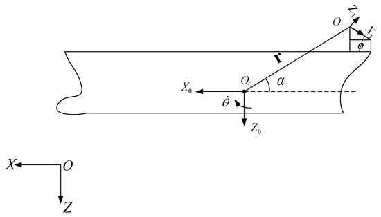
Figure 1.
The three coordinate systems are the inertial coordinate system , the coordinate system fixed on the ship, and the coordinate system fixed on the skid.
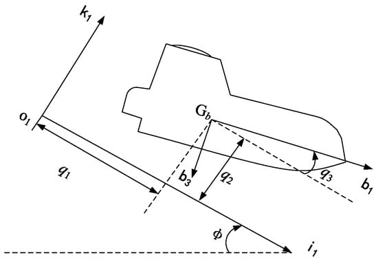
Figure 2.
Generalized coordinates of the boat in the coordinate system fixed on the skid and the coordinate system attached to the boat with the unit vectors .
2.2. Mathematical Model of Boat
The relative position of and remains unchanged in . The vector is represented by and is the angle of with the horizontal line. Based on the theorem for composited velocity and acceleration, the velocity and acceleration of are
where are the velocity and acceleration of the ship.
When considering only the ship’s longitudinal motion, the ship’s pitch angle is ; are components of the ship’s velocity in the direction of axis . The velocity and acceleration of are
The velocity and acceleration of are
The angular velocity of the rigid body is irrelevant to the choice of the base point, so . The angular velocity and acceleration of the boat are
The lifeboat is divided into cross sections with equal thickness along the length of the boat. The coordinates of the center of each section are expressed as in the coordinate system of the boat, and is the length of boat. The thickness of each section is ; the velocity at the center of each cross section is
Generalized coordinates are , generalized velocities are , partial velocities associated with points , and the angular velocity are written as follows [30]:
The force analysis of the boat at the skid is shown in Figure 3. Forces acting on the boat are gravity , supporting force , and friction .
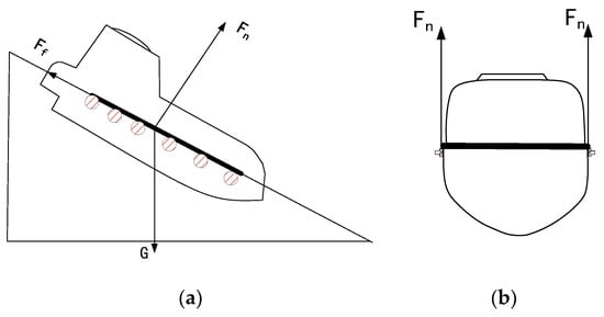
Figure 3.
The side view (a) of forces and front view (b) of supporting force acting on the boat at the skid. The lifeboat is located on the contact rollers on both sides of the skid. The top point of the rollers is in contact with the boat and provides supporting force and friction.
The generalized force of gravity and inertia are, respectively,
where is the mass of the boat, is the acceleration of gravity, and is the moment of inertia around .
For the supporting force , this paper regards the contact roller as a spring with stiffness coefficient and damping coefficient . The frictional contact force is modeled using a coefficient of . The coordinates of the center of each section are in the boat coordinate system. We define them as follows:
The velocity of each section relative to its contacting point is . The positions of each contact roller are known; there are contact rollers on each side of the skid. The coordinates of the top of the contact roller on each side of the axes of and at the skid coordinate system are as . The contacting force between and contact rollers [31,32] is
where
The associated generalized force acting on the by the skid is
The combined generalized force of the skid that acted on the boat is . The equation of the boat motion is
where . Finally, the fourth-order Runge‒Kutta method is used to solve the differential equation.
2.3. Mathematical Model of Ship Motion
Based on the model of MMG [33], the coordinate system is as shown in Figure 1. The ship dynamic equation is
where the variables with subscript are the forces and moments on the hull; the variables with subscript are wave forces. is the mass of the ship; are, respectively, added masses in the direction of the axes ; are the rotational moment of inertia around axes ; are the added moment of inertia around axes ; are velocities in the direction of axes ; and are the angular velocities around axes. ; other added masses are calculated as follows:
where is the block coefficient, is the draft, is the ship width, and is the length between perpendiculars. are calculated as follows:
where is the prismatic coefficient.
The kinematics equation is
where and are displacements and Euler angles relative to the inertial coordinate system, respectively.
The forces and moments on the hull are
where ,, are hydrodynamic derivatives, which are easily calculated according to the ship parameters [34] is the ship displacement, is the metacentric height, is the coordinate of action point of in the direction of , and is the distance between the center of gravity and the center.
For the wave force, it is estimated, based on the Frude‒Krenov assumption, that the hull is simplified to a box, and the six-degrees-of-freedom wave force and moment are as follows [34]:
where is the amplitude of the wave, is the number of waves, is the encounter frequency, is the encounter angle, is the water density, and is the ship waterline length.
The motion parameters of the ship can be obtained by solving the differential Equations (16) and (19) using the fourth-order Runge‒Kutta method.
3. Water Entry
The geometric orientation relationship of the inertial and boat coordinate system is represented by . The transformation relationship between the two coordinate systems is as follows, where is transformation matrix:
where .
The generalized coordinates are
The generalized velocities are
where are the velocity and angular velocity of the lifeboat, respectively.
The relationships between generalized coordinates and generalized velocities are
The acceleration and angular acceleration of the boat are
The partial angular velocities and velocities of the boat are
The generalized inertial force is
where is the moment of inertia around .
The generalized force caused by the gravity of the boat is
The generalized force caused by air drag is
where is the vector difference between the lifeboat velocity and the wind velocity , is the air density, is the projected area of the lifeboat in the plane perpendicular to , and is the coefficient of air drag.
The generalized force caused by fluid drag is
where is the fluid drag acting on and is the partial velocity of . The velocity of is as follows:
where .
The partial velocities of are
The components of the fluid drag acting on are as follows [22]:
where is the density of seawater and is the area of perpendicular to below the water surface. The section has maximum area , is the fluid drag coefficient, and is the component of the velocity of the section relative to the wave surface on the axis of .
The generalized force caused by buoyancy is
where is the volume of in water and is the buoyancy acting on .
The generalized force caused by the slamming force is
where is the slamming force that acted on section . Previous scholars adopted the momentum theory to calculate the slamming force. When an object enters the water, part of its initial momentum will be transferred to the surrounding water. Assuming that the momentum conversion process is irreversible, the slamming force acting on the boat can be calculated by the rate of its momentum change:
where is the velocity of the object before entering the water and is the velocity of the object after entering the water; is the mass of the object and is the added mass of the object.
Another method is based on energy theory, which was derived by Wu [35]. It has more physical significance and is widely used [36,37,38]. The relationship between slamming force and added mass is
In order to consider the effect of the wave on the boat, the incident wave force is added into the slamming force:
where is the submerged volume and is the fluid acceleration.
In this paper, the slamming force is calculated as the sum of energy theory and incident wave force for the first time. are the components of on the axis of :
where is the wave surface acceleration at section at the coordinate system of the boat, are the components of at the coordinate system of the boat, are the added mass of the cross section in the direction of , is the added mass of the boat in the direction of , and is the velocity component of the midsection between the bow and the center of gravity of the boat in the direction of .
have coordinates in an inertial coordinate system:
The depth of is
where are elements of the matrix of , the subscript is its location in the matrix, is the vertical distance from the center of gravity to the keel, is 1.15 m in Figure 4, and is a known function describing the wave surface.
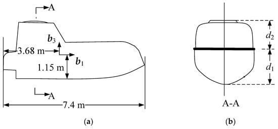
Figure 4.
Lifeboat cross section: (a) longitudinal section in center plane, (b) A‒A cross section.
The added mass is in this paper. depends on the depth and the instantaneous half width of at the wave surface:
where is half the width of at depth . When the depth of is greater than , the added mass is calculated according to the half-width at depth , as shown in Figure 4. We take the derivative of to time with
To calculate , define
where . The length of water entry in the direction of is :
where is the added mass of the boat in the direction of when the boat is completely in the water.
where is a coefficient depending on . We take the derivative of to time with
The acceleration of the section is
where
So
where is the distance from the center of gravity of the boat to the bow.
In summary, the equation of motion is
The motion parameters of the lifeboat can be solved by Equation (64) by the fourth-order Runge‒Kutta method.
4. Results and Analysis
4.1. Experimental Setup and Implementation
The basic information of the boat, ship, and skid is shown in Table 1, Table 2 and Table 3. Air drag coefficient . Fluid drag coefficient . Figure 5 gives the structural dimension diagram of the ship and boat in the simulation experiment.

Table 1.
Basic information of the boat.
Table 2.
Basic information of the ship.
Table 3.
Basic information of the skid.
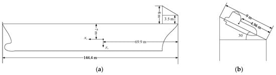
Figure 5.
Structural dimension diagram of the ship and boat: (a) the size of the longitudinal section in the center plane of the ship and skid; (b) the inclination of the skid and the position of the boat at the skid.
The simulation experiment of the whole algorithm was realized by MATLAB. The flow of the algorithm consists of two stages that are separated by the time point of the boat out of the skid. In the first stage, the motion of the skid is calculated according to parameters of ship motion solved by Equations (16) and (19). The generalized contact force can be solved by Equation (14), the generalized force caused by gravity and inertia can be solved by Equations (9) and (10), and the generalized velocities and generalized coordinates of the boat can be solved by Equation (15). In the second stage, the generalized force caused by inertial, gravity, air drag, fluid drag, buoyancy, and slamming force can be solved by Equations (32), (34), (36), (38), (44) and (47); the generalized velocities of the boat can be solved by Equation (64); and the generalized coordinates of the boat can be solved by Equations (26) and (27). For the two stages, 20 lifeboat segments were used. For convenience of analysis and understanding, the data of the boat’s translation and pitch are shown in the coordinates obtained by the inertial coordinate system, rotating 180° around the axis of .
The results of a simulation experiment by the numerical algorithm in this paper were compared with the results of Star CCM+ at the initial condition A, as shown in Table 4. The version of Star CCM+ used was 13.02. These computations were performed using an overlapping grid, as shown in Figure 6a, in order to provide accurate wave representation at any location irrespective of the lifeboat position. The behavior of two fluids (air and water) in the same continuum is modeled by using the model of volume of fluid (Figure 6b). Due to the existence of two fluids in different phases, the Euler multiphase model is activated and the gravity model is used to take into account the gravity effect of the two fluids. The initial condition of water entry is obtained by our numerical algorithm: the boat enters the water at the crest of the wave, the pitch angle of the boat when entering the water is 50.7° with horizontal, vertical, and rotational velocity of 5.9 m/s, −11 m/s, and 0.46 rad/s.
Table 4.
Details of initial condition A.
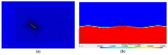
Figure 6.
Simulation experiment diagram of Star CCM+: (a) overlapping grid; (b) volume fraction of water.
4.2. Comparison and Analysis of Experimental Results
The red line is the result of the whole motion process calculated by the model in this paper. The red blue is the result of the water entry process calculated by Star CCM+.
Figure 7 shows the trajectory and pitch angle of the boat. The results show that the trajectory and pitch angle calculated by two methods are in good agreement. When the boat moves on the skid, the pitch angle begins to change with no obvious logic. The pitch angle begins to increase at the bottom of the skid. After the boat leaves the skid, the pitch angle of the boat gradually increases to about 53°. The pitch angle begin to decrease after increases in short time because the bow of the boat hits the water. The center of gravity of the boat is sinking, the bow of the boat is raised, resulting in the stern hitting the water. The buoyancy increases with the increase of the depth of the stern. Subsequently, the pitch angle of the boat begins to increase again, and the lifeboat begins to float. After it comes out of the water, the bow hits the water again.
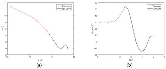
Figure 7.
Trajectory (a) and pitch (b) of the lifeboat freefall during its launch from the ship.
Figure 8 shows the ratio of the acceleration of the center of gravity to . When the boat is on the skid, the acceleration value of the center of gravity of the boat begins to vibrate. When the boat is at the low end of the skid, the vibration frequency of the acceleration value increases and the amplitude decreases. When the boat leaves the skid, the horizontal acceleration of the boat is zero and the vertical acceleration is before entering the water. The horizontal acceleration of the boat is negative in the initial stage of water entry because of the slamming force and the fluid drag force, and the acceleration becomes positive when the boat floats up because of its large buoyancy. The vertical acceleration of the boat is almost positive because of the upward force, and its negative value caused by gravity and fluid drag when the boat floats up. There is a little difference between the acceleration values calculated by the two methods, especially at the initial stage of water entry. The difference is acceptable. This phenomenon may be due to the fact that the deformation of the water caused by boat is not considered in this algorithm.
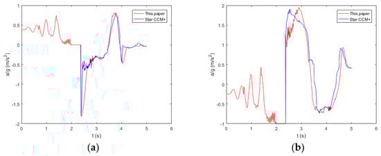
Figure 8.
Acceleration of center of gravity of the lifeboat in the horizontal (a) and vertical (b) direction.
Figure 9 shows the velocity of the center of gravity of the boat. The horizontal velocity of the boat gradually begins to increase at the skid, and remains the same in the air before entering the water; it begins to decrease due to the negative acceleration at the beginning of the water entry phase, and begins to increase when the boat floats up. The value of vertical acceleration is decreasing because the boat moves down the skid. The value of vertical acceleration decreases at the same rate because of g in the air before entering the water. Its value gradually increases until the sign is positive because of the slamming force and the buoyancy at the water entry phase; its sign becomes negative when the boat falls into the water again. The velocity values calculated by the two methods are in good agreement.
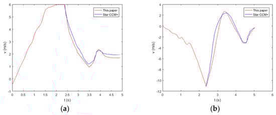
Figure 9.
Velocity of center of gravity of the lifeboat in the horizontal (a) and vertical (b) direction.
Figure 10 shows the velocity and acceleration of pitch. When the boat is on the skid, the value of the velocity of the pitch begins to vibrate. When the boat leaves the skid, the velocity of the pitch remains the same before entering the water. The velocity of the pitch decreases to a negative value when the boat enters the water. Its sign is positive when the boat’s bow begins to fall into the water again. The acceleration of the pitch has the same rule of change as the horizontal acceleration. The velocity and acceleration of pitch calculated by the two methods are in good agreement.
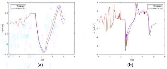
Figure 10.
Velocity (a) and acceleration (b) of pitch of the lifeboat.
In summary, the position and velocity of the center of gravity of the boat, the angle, and velocity and acceleration of pitch calculated by the two methods are in good agreement. There is a little difference between the values of translation acceleration calculated by the two methods. The difference is acceptable. This shows that the numerical algorithm in this paper has good accuracy.
The boat experiences three water impacts (bow impact, stern impact, bow impact) in the previous analysis. In order to analyze the local acceleration of different positions in the boat, the local acceleration of the bow, midship, and stern is calculated by Equation (1). Figure 11 shows the acceleration of the bow (a,b), midship (c,d), and stern (e,f) in the boat coordinate system. The acceleration values in all figures are the ratio of actual values to the acceleration of gravity .
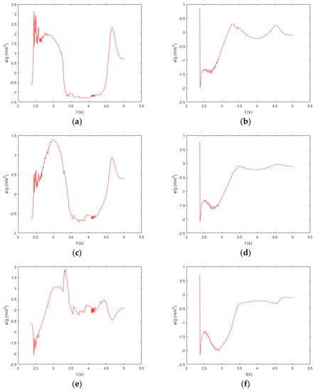
Figure 11.
The acceleration of the bow, midship, and stern in the coordinate system of the lifeboat in the direction of (a,c,e) and in the direction of (b,d,f).
During the whole water entry process, the acceleration curves have three peaks because of three water impacts (Figure 11a,c) The first two peaks are close; there is a positive maximum acceleration in the direction of at the bow at the first impact as the first peak of the curve (Figure 11a). There is a positive maximum acceleration in the direction of at the midship at the second impact as the second peak of the curve (Figure 11c). There are two contrary extreme values of the acceleration at the stern in the direction of (Figure 11e): a negative extremum due to the first impact, and a positive extreme value due to the second impact. The negative maximum acceleration in the direction of at the bow, midship, and stern is because of the first impact (Figure 11b,d,f). The maximum acceleration is about 3 in the direction of , derived from the bow’s first impact.
4.3. Qualitative Analysis
According to the numerical calculation method used in this paper, the local acceleration extremum is calculated under different initial conditions. The wave heights are 1, 2, 3, 4, and 5 m. By adjusting the initial phase of the wave, the points of water entry of the boat are shown in Figure 12. Figure 12a shows the ship heading the wave and Figure 12b shows the ship following the wave. When the ship is heading or following the wave, only the surge, heave, and pitch of the ship are considered. Other initial conditions (period of wave, wind velocity, ship’s initial position, ship’s initial velocity) are the same as in condition A.
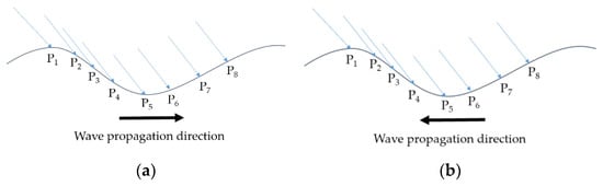
Figure 12.
Eight different points of water entry of the boat when the ship is heading the wave (a) and following the wave (b).
Figure 13, Figure 14, Figure 15, Figure 16 and Figure 17 show the trajectory and pitch angle of the lifeboat when the ship is heading the wave. Figure 18 shows the maximum value of the acceleration in the directions of and at the bow (Figure 18a,b), midship (Figure 18c,d), and stern (Figure 18e,f) of the boat at eight different points of water entry when the ship is heading waves. Figure 19, Figure 20, Figure 21, Figure 22 and Figure 23 show the trajectory and pitch angle of the lifeboat when the ship is following waves. Figure 24 shows the maximum value of the acceleration in the directions of and at the bow (Figure 24a,b), midship (Figure 24c,d), and stern (Figure 24e,f) of the boat at eight different points of water entry when the ship is following waves. As there are no experimental data for comparison, the numerical calculation results may not be very accurate, but can be used in a qualitative analysis.
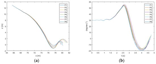
Figure 13.
Trajectory (a) and pitch (b) of the lifeboat freefall when the wave height is 1 m.
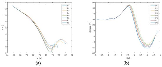
Figure 14.
Trajectory (a) and pitch (b) of the lifeboat freefall when the wave height is 2 m.
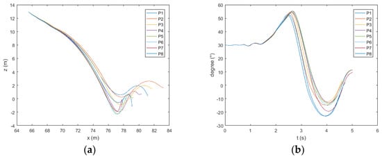
Figure 15.
Trajectory (a) and pitch (b) of the lifeboat freefall when the wave height is 3 m.
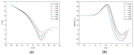
Figure 16.
Trajectory (a) and pitch (b) of the lifeboat freefall when the wave height is 4 m.
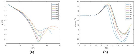
Figure 17.
Trajectory (a) and pitch (b) of the lifeboat freefall when the wave height is 5 m.
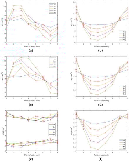
Figure 18.
The maximum acceleration of the bow, midship, and stern in the coordinate system of the lifeboat in the direction of (a,c,e), and in the direction of (b,d,f), at different wave heights.
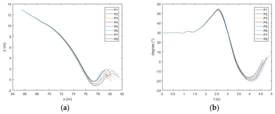
Figure 19.
Trajectory (a) and pitch (b) of the lifeboat freefall when the wave height is 1 m.
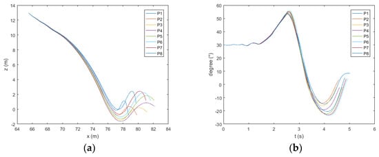
Figure 20.
Trajectory (a) and pitch (b) of the lifeboat freefall when the wave height is 2 m.
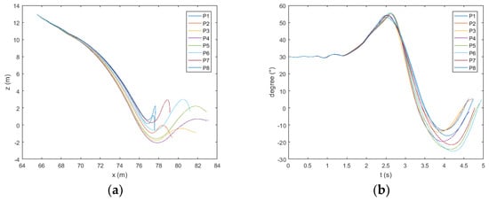
Figure 21.
Trajectory (a) and pitch (b) of the lifeboat freefall when the wave height is 3 m.
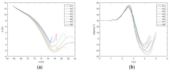
Figure 22.
Trajectory (a) and pitch (b) of the lifeboat freefall when the wave height is 4 m.
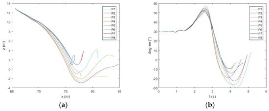
Figure 23.
Trajectory (a) and pitch (b) of the lifeboat freefall when the wave height is 5 m.
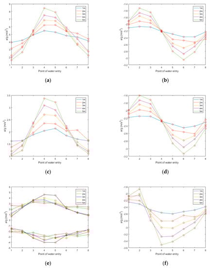
Figure 24.
The maximum acceleration of the bow, midship, and stern in the coordinate system of the lifeboat in the direction of (a,c,e), and in the direction of (b,d,f), at different wave heights.
The ship heads the wave. As shown in Figure 15, Figure 16 and Figure 17a, when the wave height exceeds 3 m, the boat will move to the side of the ship after water entry at P7 and P8. As shown in Figure 16a and Figure 17a, when the wave height exceeds 4 m, the same phenomenon appears at point P6. As shown in Figure 13, Figure 14, Figure 15, Figure 16 and Figure 17b, at points P1 and P8, the pitch angle of the boat has a large range of change. As shown in Figure 18, in the direction of , the maximum values of acceleration at the bow, midship, and stern of the boat appear at point P4; the minimum value generally appears at P1 and P8. The maximum values at the bow and midship are almost the same, slightly lower than the stern. In the direction of , the maximum absolute values of acceleration at the bow and midship of the boat appear at points P3 and P2; the minimum value generally appears at points P7 and P8. There is no obvious rule about the values of acceleration at the stern; the acceleration is the largest at the bow and the smallest at the midship.
The ship follows the wave. As shown in Figure 21, Figure 22 and Figure 23a, when the height of the wave exceeds 3 m, the boat will move to the side of the ship after water entry at points P1 and P8. As shown in Figure 22 and Figure 23a, when the height of the wave exceeds 4 m, the same phenomenon appears at point P7. As shown in Figure 19, Figure 20, Figure 21, Figure 22 and Figure 23b, the pitch angle of the boat has a large range of change at points P5 and P6. As shown in Figure 24, in the direction of , the maximum values of acceleration at the bow and midship appear at points P6 and P7, and the minimum values generally appear at points P2 and P3. The maximum values of acceleration at the stern appear at points P4 and P5, and the minimum values generally appear at points P1 and P2. The maximum values at the bow and midship of the boat are almost the same, and slightly lower than for the stern. In the direction of , the maximum values of acceleration at the bow and midship of the boat appear at points P4 and P5; the minimum value generally appears at points P1 and P8. The maximum absolute values of the two extremal values at the stern appear at P4 and P5. The minimum values generally appear at P1 and P8; the acceleration is the largest at the bow and the smallest at the midship.
Therefore, when the ship is heading the wave, P7 and P8 can be selected to enter the water at a low wave. In order to prevent the boat from moving to the side, one can choose point P1 at a high wave, which will withstand a large change in pitch. When the ship is following the wave, P1 and P8 can be selected at a low wave. In order to prevent the boat moving to the side, one can choose P2 and P3 at a high wave. In summary, it is safer to select points at the crest and behind the crest when entering the water.
5. Application
This paper applies an established mathematical model to a ship’s lifesaving training system, improving the immersion and reality of the system. The system takes the Panama bulk carrier as a physical prototype, and uses 3D Studio Max (3ds Max) to build 3D models of the ship, lifeboat, and skid. The system constructs a virtual scene of a ship life-saving drill, and releases the lifeboat through a three-dimensional virtual operation, as shown in Figure 25.
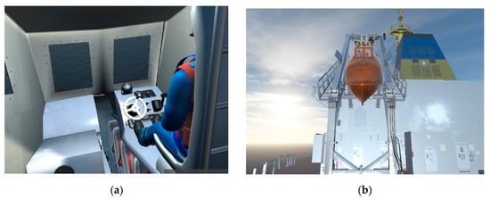
Figure 25.
Scene of virtual human operating lifeboat (a) and lifeboat moving on the skid (b) in a ship’s lifesaving training system.
6. Conclusions
This paper presents a computational model for the simulation of lifeboat freefall during its launching from a ship in rough seas. The model is applied to the ship’s lifesaving training system. We can draw the following conclusions:
- (1)
- The mathematical model in this paper can simulate the entire process of the water entry of the ship’s lifeboat and can acquire the parameters of the boat’s trajectory, pitch angle, velocity, local acceleration, etc.
- (2)
- The results of a numerical simulation experiment are compared with the calculation results of the hydrodynamics software Star CCM+ at water entry under initial condition A. It shows that our numerical algorithm has good accuracy. The model can be applied to other ships by adjusting the parameters.
- (3)
- Under different wave heights and two situations of the ship encountering waves, a qualitative analysis is performed to determine the safe point of water entry. It is safer to select points at the crest and behind the crest when entering the water.
- (4)
- Since the motion of the boat on the skid is only three-degrees-of-freedom, the effects of the ship’s roll, sway, and yaw are not considered; only the simulation experiments of the ship heading and following the wave are analyzed. Future research will consider the effect of the ship’s roll, sway, and yaw.
Author Contributions
S.Q. led the writing of the manuscript, contributed to data analysis and research design, and serves as the corresponding author. H.R. supervised this study, contributed to the funding acquisition, and serves as the corresponding author. H.L. contributed to the investigation and corrected the format of the paper. All authors have read and agreed to the published version of the manuscript.
Funding
The authors are thankful for the financial support provided by National Natural Science Foundation of China (Grant No. 51679024), the Fundamental Research Funds for the Central Universities (Grant No. 3132020372), and Natural Science Foundation Guidance Project of Liaoning Province (Grant No. 2019-ZD-0152).
Conflicts of Interest
The authors declare no conflict of interest.
References
- Nelson, J.K., Jr.; Waugh, P.J.; Schweickhardt, A.J. Injury criteria of the IMO and the Hybrid III dummy as indicators of injury potential in free-fall lifeboats. Ocean Eng. 1996, 23, 385–401. [Google Scholar] [CrossRef]
- Billard, R.; Musharraf, M.; Veitch, B.; Smith, J. Using Bayesian methods and simulator data to model lifeboat coxswain performance. WMU J. Mar. Aff. 2020, 1–18. [Google Scholar] [CrossRef]
- Qiu, S.; Ren, H. Ship Life-Saving Training System Based on Virtual Reality Technology. In Proceedings of the 2018 IEEE 4th International Conference on Control Science and Systems Engineering, Wuhan, China, 21–23 August 2018; pp. 559–563. [Google Scholar]
- Billard, R.; Smith, J.; Veitch, B. Assessing Lifeboat Coxswain Training Alternatives Using a Simulator. J. Navig. 2019, 1–16. [Google Scholar] [CrossRef]
- Re, A.S.; MacKinnon, S.; Veitch, B. Free-Fall Lifeboats: Experimental Investigation of the Impact of Environmental Conditions on Technical and Human Performance. In Proceedings of the 27th ASME International Conference on Offshore Mechanics and Arctic Engineering, Estoril, Portugal, 15–20 June 2008; pp. 81–88. [Google Scholar] [CrossRef]
- Re, A.S.; Veitch, B. A comparison of three types of evacuation system. Trans. Soc. Nav. Archit. Mar. Eng. 2007, 115, 119–139. [Google Scholar]
- Re, A.S.; Veitch, B. Experimental investigation of free-fall lifeboat performance. In Proceedings of the 17th 2007 International Offshore and Polar Engineering Conference, Lisbon, Portugal, 1–6 July 2007; pp. 3608–3615. [Google Scholar]
- Hollyhead, C.J.; Townsend, N.C.; Blake, J.I.R. Experimental investigations into the current-induced motion of a lifeboat at a single point mooring. Ocean Eng. 2017, 146, 192–201. [Google Scholar] [CrossRef]
- Hwang, J.K.; Chung, D.U.; Ha, S.; Lee, K.Y. Study on the safety investigation of the free-fall lifeboat during the skid-launching test. In Proceedings of the IEEE OCEANS 2012—Yeosu, Yeosu, Korea, 21–24 May 2012. [Google Scholar] [CrossRef]
- Mørch, S.E.H.; Peric, M.; Schreck, E. Simulation of Lifeboat Launching under Storm Conditions. In Proceedings of the 6th International Conference on CFD in Oil and Gas, Trondheim, Norway, 10–12 June 2008. [Google Scholar]
- Tregde, V.; Nestegrd, A. Prediction of Irregular Motions of Free-Fall Lifeboats during Drops from Damaged FPSO. In Proceedings of the ASME 2014 33rd International Conference on Ocean, Offshore and Arctic Engineering, San Francisco, CA, USA, 8–13 June 2014. [Google Scholar]
- Ringsberg, J.; Heggelund, S.; Lara, P.; Jang, B.S.; Hirdaris, S.E. Structural response analysis of slamming impact on free fall lifeboats. Mar. Struct. 2017, 54, 112–126. [Google Scholar] [CrossRef]
- Abrate, S. Hull Slamming. Appl. Mech. Rev. 2011, 64, 060803. [Google Scholar] [CrossRef]
- Zakki, A.; Fauzan, A.; Bae, D.M.; Myung, D. The development of new type free-fall lifeboat using fluid structure interaction analysis. J. Mar. Sci. Technol. 2016, 24, 575–580. [Google Scholar] [CrossRef]
- Nelson, J.K.; Hirsch, T.J.; Phillips, N.S. Evaluation of Occupant Accelerations in Lifeboats. ASME J. Offshore Mech. Arct. Eng. 1989, 111, 344–349. [Google Scholar] [CrossRef]
- Karman, V. The Impact on Seaplane Floats during Landing; National Advisory Committee for Aeronatics, NO.321; NACA: Seattle, WA, USA, 1929; pp. 1–8. [Google Scholar]
- Boef, W.J.C. Launch and impact of free-fall lifeboats. Part I. Impact theory. Ocean Eng. 1992, 19, 119–138. [Google Scholar] [CrossRef]
- Boef, W.J.C. Launch and impact of free-fall lifeboats. Part II. Implementation and applications. Ocean Eng. 1992, 19, 139–159. [Google Scholar] [CrossRef]
- Arai, M.; Khondoker, M.R.H.; Inoue, Y. Water Entry Simulation of Free-fall Lifeboat (First Report: Analysis of Motion and Acceleration). Nihon Zosen Gakkai Ronbunshu 1995, 178, 193–201. [Google Scholar] [CrossRef]
- Arai, M.; Khondoker, M.R.H.; Inoue, Y. Water Entry Simulation of Free-fall Lifeboat (2nd Report: Effects of Acceleration on the Occupants). Nihon Zosen Gakkai Ronbunshu 1995, 179, 205–211. [Google Scholar]
- Khondoker, M.R.H.; Khalil, G. Effect of guide rail on the motion and acceleration of a free-fall lifeboat. Indian J. Eng. Mater. S 1998, 5, 49–54. [Google Scholar]
- Khondoker, M.R.H. Effects of Launching Parameters on the Performance of a Free-Fall Lifeboat. Nav. Eng. J. 2009, 110, 67–73. [Google Scholar] [CrossRef]
- Khondoker, M.R.H.; Arai, M. A comparative study on the behaviour of free-fall lifeboat launching from a skid and from a hook. Proc. Inst. Mech. Eng. Part C J. Mech. Eng. 2000, 214, 359–370. [Google Scholar] [CrossRef]
- Karim, M.M.; Iqbal, K.S.; Khondoker, M.R.H. Numerical investigation into the effect of launch skid angle on the behaviour of free-fall lifeboat in regular waves. Trans. RINA Part B1 Intl. J. Small Craft Tech. 2009, 151, 37–48. [Google Scholar]
- Karim, M.M.; Iqbal, K.S.; Khondoker, M.R.H.; Rahman, S.M.H. Influence of falling height on the behavior of skid- launching free-fall lifeboat in regular waves. J. Appl. Fluid Mech. 2012, 4, 77–88. [Google Scholar]
- Raman-Nair, W.; White, M. A model for deployment of a freefall lifeboat from a moving ramp into waves. Multibody Syst. Dyn. 2013, 29, 327–342. [Google Scholar] [CrossRef]
- Faltinsen, O.M. Sea Loads on Ships and Offshore Structures; Cambridge University Press: Cambridge, UK, 1990; pp. 300–306. [Google Scholar]
- Sumer, B.M.; Fredsoe, J. Hydrodynamics around Cylindrical Structures; World Scientific: Singapore, 1997; pp. 123–201. [Google Scholar]
- Dymarski, C.; Dymarski, P. Computational simulation of motion of a rescue module during its launching from ship at rough sea. Pol. Marit. Res. 2014, 21, 54–60. [Google Scholar] [CrossRef]
- Kane, T.R.; Likins, P.W.; Levinson, D.A. Spacecraft Dynamics; McGraw Hill Inc.: New York, NY, USA, 1983; p. 30. [Google Scholar]
- Uğur, G.; Bülent, Ö.; Yilmaz, T. A spring force formulation for elastically deformable models. Comput. Graph. 1997, 21, 335–346. [Google Scholar] [CrossRef]
- McMillan, A.J. A non-linear friction model for self-excited vibrations. J. Sound Vib. 1997, 205, 323–335. [Google Scholar] [CrossRef]
- Jia, X.; Yan, G.Y. Ship Motion Mathematical Model: The Mechanism Modeling and Identification Modeling; Dalian Maritime University Press: Dalian, China, 1999; pp. 49–138. [Google Scholar]
- Mo, J. Numerical Simulation of Ship Maneuvering Motion with Six Degree of Freedom in Waves. Master’s Thesis, Harbin Engineering University, Harbin, China, 2009. [Google Scholar]
- Wu, G. Hydrodynamic force on a rigid body during impact with liquid. J. Fluid Struct. 1998, 12, 549–559. [Google Scholar] [CrossRef]
- Cointe, R.; Fontaine, E.; Molin, B.; Scolan, Y.M. On energy arguments applied to the hydrodynamic impact force. J. Eng. Math. 2004, 48, 305–319. [Google Scholar] [CrossRef]
- Casetta, L.; Pesce, C.P.; Flávia, M.D.S. On the hydrodynamic vertical impact problem: An analytical mechanics approach. Mar. Syst. Ocean Technol. 2011, 6, 47–57. [Google Scholar] [CrossRef]
- Scolan, Y.; Korobkin, A.A. Energy distribution from vertical impact of a three dimensional solid body onto the flat free surface of an ideal fluid. J. Fluids Struct. 2003, 17, 275–286. [Google Scholar] [CrossRef]
© 2020 by the authors. Licensee MDPI, Basel, Switzerland. This article is an open access article distributed under the terms and conditions of the Creative Commons Attribution (CC BY) license (http://creativecommons.org/licenses/by/4.0/).