Abstract
Liquefied natural gas began to attract attention as a ship fuel to reduce environmental pollution and increase energy efficiency. During this period, highly efficient internal combustion engines emerged as the new propulsion system instead of steam turbines. However, Otto-cycle engines must use fuel that meets the methane number that was given by the engine makers. The purpose of this study was to develop a system configuration and a control method of methane number adjustment using combined cascade/feed-forward controllers for marine Otto-cycle engines to improve reference tracking and the disturbance rejection. The main principle involves controlling the downstream gas temperature of the fuel gas supply system to meet the required methane number. Three controllers are used in the combined cascade/feed-forward control for adjusting the downstream of the gas temperature: the cascade loop has two controllers and the feed-forward has one controller. The two controllers in the cascade loop are designed with proportional–integral (PI) controllers. The remaining controller is based on feed-forward control theory. A simulation was conducted to verify the efficacy of the proposed method, focusing on the disturbance rejection and set-point tracking, in comparison with a single PI controller, a single PI controller with feed-forward, and cascade control.
1. Introduction
The International Maritime Organization (IMO) has adopted regulations to address the emission of air pollutants from ships and has implemented mandatory energy efficiency measures to reduce the emissions of greenhouse gases from shipping, under the International Convention for the Prevention of Pollution from Ships (MARPOL). First, sulphur oxides (SOx) and nitrogen oxides (NOx) were reduced as a solution to air pollution. Second, the energy efficiency design index (EEDI) was made mandatory for new ship’ construction as adopted by MARPOL [1,2,3]. In other words, it will increase energy efficiency to reduce environmental pollution. The final goal of these two items is to reduce pollutants and minimize fuel use.
For that reason, liquefied natural gas (LNG) began to attract attention as a ship fuel [4,5]. During this period, various gas engines using natural gas (NG) for marine purpose emerged as new propulsion systems with high efficiency and low operational costs instead of steam turbines [6]. In other words, the Otto-cycle engine, which is one of the gas engine types, has begun to replace the existing ship propulsion system, the steam turbines. Figure 1 shows the concept of the Otto-cycle engines. During compression stroke in the Otto-cycle engines, low-pressure fuel gas is injected from the middle of the cylinder liner to perform the compression stroke in the premixed state with the scavenging air. Then, at the end of the compression stroke, combustion proceeds by injecting the fuel for the ignition through fuel valves installed on the upper part of the cylinder head.
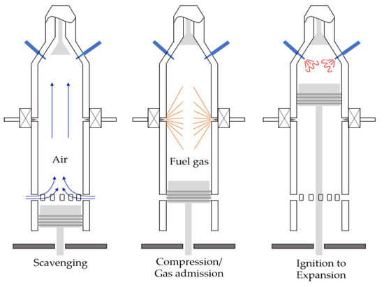
Figure 1.
The concept of the Otto-cycle engines [7].
However, the Otto-cycle engine has the disadvantage of having to meet the proper methane number (MN) that was given by the engine makers. On average, values of 60–80 are provided. The MN describes the ability of NG to withstand compression before ignition. Pure methane has a MN of 100, and pure hydrogen has a MN of 0. Fuels with lower methane numbers pose performance problems for fuel gas supply systems (FGSSs) due to combustion knocking caused by higher amounts of ethane, propane, and heavier hydrocarbons [8]. Major causes of low MN are LNG ageing, temperature rise of the cargo tank inside, and low MN LNG forced vaporization [9]. A list of the LNG composition and MN available from some LNG terminals is provided in Table 1. With the low MN of LNG supplied from the LNG terminal, it is highly likely that the MN will be lower due to the increase in the temperature of the cargo tank and LNG ageing while sailing, which means that a system capable of controlling the MN is needed.

Table 1.
Liquefied natural gas (LNG) compositions and methane number (MN) at some LNG terminals.
The primary contribution of this study is the development of a system configuration and a methane number adjustment control method for marine Otto-cycle engines to improve reference tracking as well as the disturbance rejection with combined cascade/feed-forward controllers. First of all, we suggest how to adjust the MN using existing equipment in current LNG carriers (LNGCs) and LNG-fueled ships (LFSs). Some research has focused on calculation methods and test methods of the methane number. Partho et al. [8] developed a prediction model of the natural gas methane number. Martin et al. [10] studied methane number test of the alternative gaseous fuels. However, a method for controlling the MN in ships’ Otto-cycle engines was needed. The method focusing on the fact that each gas has a different boiling point was applied in this paper in order to control the MN of the natural gas.
Then, appropriate control methods could be applied in MN control systems. Feed-forward control and cascade control are considered two of the proper control methods. Feed-forward control is used to ensure constant control performance when a disturbance affects a process under feedback control. The weak point of feedback control is that a process variable (PV) is necessary before a manipulated variable (MV) change is taken when a disturbance affects a process. The application of feed-forward control is sufficient to compensate for this weakness. However, the performance of feed-forward control is limited by model uncertainty [11]. In practice, the disturbance rejection and accuracy of the system response are important. Cascade control was adapted to show how to use multiple process variables to improve the response to a disturbance and reference tracking.
Several studies focused on control methods using cascade control and feed-forward control. Lee et al. [12] suggested the use of internal model controller (IMC) principles as a controller tuning method for both inner and outer loop controllers in cascade control. Kaya [13,14] proposed the application of the Smith predictor scheme in a long time delay system. Some researchers [15,16,17,18] studied feed-forward control with a feedback control system using advanced tuning methods such as robust control. Although many papers focused on controller tuning, others studied performance improvement by combining two types of controllers. Nguyen et al. [19] constructed a method combining an adaptively feed-forward neural controller and a proportional–integral–derivative (PID) controller to control the joint-angle position of robots.
To be applied to a ship’s control system, stability must be ensured, and controllers should be easy to tune via modification by the crew of the ship. Considering these points, combined cascade/feed-forward control is suggested with a control strategy and configuration for a MN control system in this paper. Simple tuning methods using Ziegler–Nichols, Tyreus–Luyben, and rule of thumb were applied. Using MATLAB simulation results, the performances of a single PI control, PI control with feed-forward, cascade control, and combined cascade/feed-forward control were determined and compared.
2. System Configuration and Model
The proposed MN control system shown in Figure 2 consists of an orifice, an in-line mixer, a flow control valve, an LNG supply pump, and a separator. The main idea to remove C2+, such as ethane and butane, which lowers MN from NG, is to spray cold LNG to NG to lower the temperature of the fluid stream. If the cargo tank temperature is near −80 °C, taking into account the boiling point of each gas, an in-line mixer should be operated to remove C2+ from the NG. For use of the in-line mixer, valves 2 and 3 are opened and valve 1 is closed. When the temperature of NG is lowered to about −100 °C, C2+ may condense. As opposed to the use of an in-line mixer, valve 1 is opened, and valves 2 and 3 are closed. The condensed gas is divided inside of a separator and returned to the cargo tank, and only NG with a high MN value is sent to the fuel gas supply system. The high MN gas is supplied to Otto-cycle engines through the fuel gas supply system, which is effective in preventing phenomena such as knocking. It is advantageous from an OPEX perspective. In addition, this Otto-cycle engine has an inherent to reduce the formation of NOx by up to 90% compared to the diffusion combustion of the diesel [7].
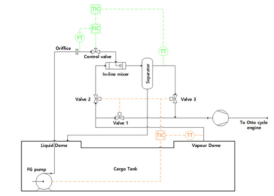
Figure 2.
Schematic diagram of the methane number (MN) control system.
2.1. Block Diagram of Combined Cascade/Feed-Forward Control
In the combined cascade/feed-forward control strategy shown in Figure 3, the temperature control is the primary control loop and the flow control is the secondary control loop. Table 2 shows the description of the block diagram. When a disturbance occurs in this system, a feed-forward controller rapidly acts to compensate for it in the system. On-off control for motor and hydraulic valves (valves 1–3) was excluded in the simulation in this study. The primary disturbance (NG inlet temperature change from cargo tanks) directly affects the primary output (the process outlet temperature of the NG controlled by an in-line mixer) without a direct impact on the secondary output (LNG flowrate from the pump). The secondary disturbance (LNG fluctuation from FG pumps of the cargo tanks in Figure 2) creates the effect on the secondary output (flowrate is adjusted by a control valve). Therefore, we adopted series cascade control instead of parallel cascade control because it is useful when the secondary process, such as the LNG flowrate, is naturally separated from the primary process [13,20].
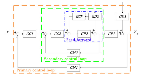
Figure 3.
Block diagram of the MN control system.
Table 2.
Description of block diagram abbreviations.
2.2. System Modelling
2.2.1. Flowmeter and Temperature Sensor
The flow control system consists of a flowmeter, a differential pressure cell, a P/I (pressure to current) transducer, a flow controller, an I/P (current to pressure) transducer, and a control valve actuator, as shown in Figure 4.
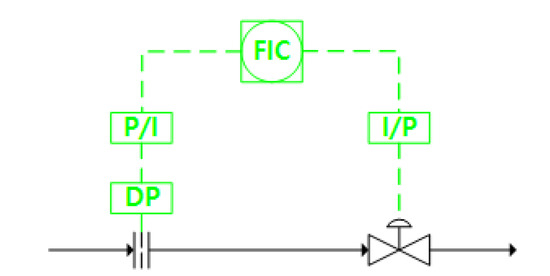
Figure 4.
Instrumentation diagram for flow control.
The input to the flowmeter can be thought of as the actual flowrate of the process fluid. The volumetric flowrate is related to the pressure drop across the orifice. Based on the Bernoulli equation and the continuity equation, the differential pressure equation is represented in Equation (1) [21]. This is modified as Equation (2) using information on the process data.
where ρ is density; is the differential pressure; Cd is the discharge coefficient (0.995); B is the ratio of orifice to pipe diameter D1/D2 (0.3895); D1 is the inner pipe diameter (0.0547878 mm); D2 is the orifice inner diameter (0.0213425 mm); and m is the mass flowrate (kg/h).
This equation for the differential pressure across the orifice is described in Figure 5. When comparing the pressure loss of a pipe to the orifice pressure loss in this paper, the two values are almost the same, which can be considered a pipe.

Figure 5.
Differential pressure across the orifice.
Focusing on the temperature sensor of the separator downstream, this can also be considered a piping line for the same reason as the orifice. Therefore, this cannot have any impacts on the system during the performance check in this study.
2.2.2. In-line Mixer
An in-line mixer is used for lowering the NG temperature against the low MN. The temperature is lowered by the spray of LNG using the nozzle into the NG. An in-line mixer consists of a nozzle for LNG spraying and a cylindrical mixing vessel, as shown in Figure 6.
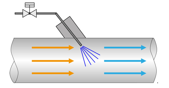
Figure 6.
Configuration of the in-line mixer [22].
The in-line mixer property is indicated by the temperature curve for adjusting the LNG mass flowrate, which can ensure the downstream temperature of the in-line mixer for the NG is −100 °C, ensuring the MN is 80 or above. For simulating how much LNG is required for cooling the NG, HYSYS (Aspen Technology, Massachusetts, USA) dynamic simulation is used. The NG mass flowrate is calculated based on cargo tanks’ maximum boiled-off rate (BOR) in the stable tank condition, referring to Gaztransport & Technigaz (GTT) information [23]. When the flowrate of the NG generated from the cargo tanks flows to the in-line mixer, the LNG flowrate that must meet the MN is sprayed through the nozzle. The temperature trend curve of the in-line mixer downstream was implemented in an HYSYS dynamic simulation, as shown in Figure 7. This curve was transformed into Equation (11) using system identification in MATLAB Simulink (MathWorks, Massachusetts, USA). For creating a transfer function of the in-line mixer, time domain data were used with the same time interval. The measured input (LNG mass flowrate) and the measured output (downstream temperature of the in-line mixer) were the independent variables, and the dependent variables were the predicted outputs. Equation (3) can be used to predict the parameters of the model [24,25,26].
where y is the measured output variable, is the parameters of the model to be determined, and is the known function called the regressor. The vectors are introduced in Equations (4) and (5).
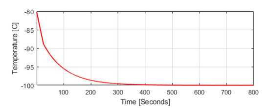
Figure 7.
Temperature curve of the downstream of an in-line mixer.
The model is indexed by the time interval. In this study, the time interval was 1 s.
During the calculation, should be chosen to minimize the least-square loss in Equation (7).
Equation (7) can be changed to Equation (8) using the notation of residuals;
where residual is defined by
and is the predicted output of the system from Equation (9). The solution to the least-squares considering the matrix is nonsingular, given by:
This model, using Equations (3)–(10), is given by:
2.2.3. Control Valve
The control valve is an important element in process industries. If the actual LNG flow is not properly controlled, even if the measurement is good, problems will arise in temperature control. The flow coefficient (Cv) is the key element for controlling the valve with the proper opening ratio. If the flow coefficient is higher than the system requirement, the control valve cannot be operated properly. This means that the temperature control fails because a large control valve can allow large amounts of LNG to cool the boil-off gas (BOG) with small movements of the actuators. Therefore, the characteristic curve of the control valve is used for making a transfer function. The characteristic curve of the control valve indicates the relationship between the flow rate through the valve and the position of the stem that changes the valve from 0% to 100% [27].
Figure 8 shows the flow characteristic curve of the control valve. The system identification and HYSYS dynamic simulation used for the in-line mixer modeling were applied to obtain the transfer function of the control valve. Equation (12) was obtained as a result of this simulation.
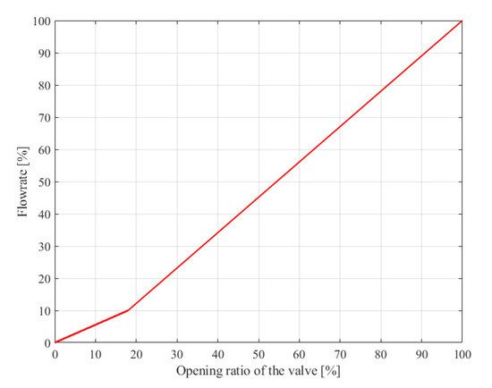
Figure 8.
Characteristic curve of the control valve.
2.2.4. Disturbance
Disturbances can occur for both the primary control loop and the secondary control loop. A primary disturbance is caused from abrupt temperature changes in the NG of cargo tanks. The abrupt temperature change can be ignored considering the size of the cargo tanks of LNG carriers. The cargo tank size of an LNGC currently varies from 140,000 to 260,000 m3. Figure 9 shows the temperature changes in a cargo tank of an actual LNGC equipped with 140,000 m3 cargo tanks. The average temperature for six days changed from −158.88 to −158.56 °C. Considering this trend of temperature change, we assumed that primary disturbance could be ignored.
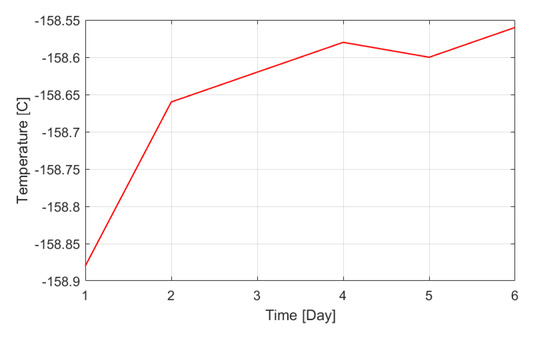
Figure 9.
Temperature curve at a cargo tank for six days in an LNG carrier.
The other disturbance type is secondary disturbance. The LNG flow from the FG pump in the cargo tanks may fluctuate. A small amount of LNG is required in the in-line mixer, but a large amount of flow may be sent to the in-line mixer when the flow control of the discharge of the FG pump fails. In addition, if the constant flow control fails downstream of the FG pump, the LNG flowrate may fluctuate significantly. This phenomenon impacts the temperature control of the separator downstream. In other words, if a large amount of LNG is suddenly injected into the NG through the in-line mixer nozzle, controlling the temperature becomes difficult. The LNG flowrate is related to the characteristic curve of the FG pump, which is shown in Figure 10.
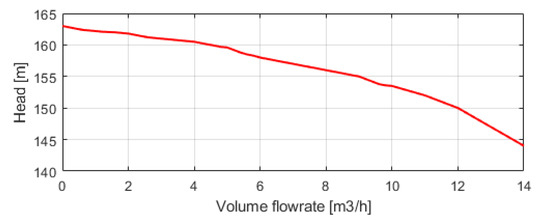
Figure 10.
Characteristic curve of the FG pump.
Mass flowrate over time was determined using HYSYS dynamic simulation for the initial start of the FG pump using the characteristic curve of this pump. Figure 11 shows how much LNG is sprayed at the in-line mixer for adjusting the NG temperature. The actual mass flowrate requested for MN control ranges from 0 to about 160 kg/h. During this cooling, the sampling time applied is 0.2 s. The transfer function of the secondary disturbance can be inferred from Equation (13) using the system identification in Figure 11.
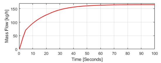
Figure 11.
LNG mass flowrate injected at an in-line mixer.
3. Controller Design
Cascade control is the most popular and commonly available method used for the rejection of disturbances arising in the secondary loop and improving the accuracy of the system response [28]. In this study, a cascade control structure with PI controllers was used to adjust the MN to the Otto-cycle engine requirements. Feed-forward control was then applied considering the flowrate fluctuation of the pump. The advantage of using feed-forward control is its quicker compensation of error compared with feedback control. Based on these advantages, we applied combined cascade/feed-forward controllers.
3.1. Cascade Controller
Tuning the cascade controllers involves two steps. First, the secondary controller must be tuned with the secondary control loop. Once the secondary control loop is finished, the transfer function of the primary control loop can be used for tuning the primary loop controller. Following this procedure, these PI controllers were adjusted using the Ziegler–Nichols method (ZN), Tyreus–Luyben method (TL), and rule of thumb (ROT) used in industry.
Using Equation (14), a secondary controller in PI form is applied.
where is the proportional gain and is integral time.
The ZN tuning method and the TL tuning method of closed loops in Table 3 were used to obtain the controller parameters for critical gain kcu and critical period Pu.
Table 3.
Summary of controller tuning parameters.
The parameter values for the PI controllers in the secondary loop are summarized in Table 4.
Table 4.
Summary of parameter values for secondary loop controller.
Equation (14) applies equally to the main controller. The tuning method used in this paper was the same procedure as applied to the secondary controller. A summary of parameter values of primary controllers is provided in Table 5.
Table 5.
Summary of parameter values for primary loop controller.
3.2. Feed-forward Controller
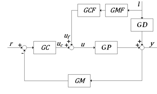
Figure 12.
Block diagram of feed-forward control.
Considering the process variable does not change, (s) is equivalent to 0. r(s) can be considered zero because there is no set point change. Based on r(s) and (s) being equivalent to zero, Equations (17) and (18) can be derived from Equation (16).
If the disturbance measurement has no dynamics, Equation (17) can be obtained as:
4. Simulation Results
A total of four types of controllers, a single PI controller, a PI controller with feed-forward (FF), cascade controllers, and combined cascade/feed-forward controllers, were reviewed with a step response. We then checked the efficiency of disturbance rejection with these controllers. The performance measurement was based on the integral of the absolute value of the error (IAE), integral of the time weight absolute value of the error (ITAE), overshoot (OS), and settling time (ST). In this study, simulation time was 10 s for the case without disturbance and 100 s for the case with a disturbance. IAE and ITAE are defined in Equations (21) and (22), respectively.
4.1. Comparison between a Single PI Controller, a Single PI Controller with Feed-Forward, and Cascade Controllers
We first examined reference tracking using a step signal. The tracking results without the disturbance should be almost same between a single PI controller and cascade controllers tuned by ROT. However, to clearly differentiate the performance of the controller against disturbance, the performance of the single controller without disturbance should be better than cascade controllers as shown in Figure 13. We did not directly compare the single PI controller with feed-forward and cascade controllers, but the findings show how effective these two controllers are in eliminating a disturbance.
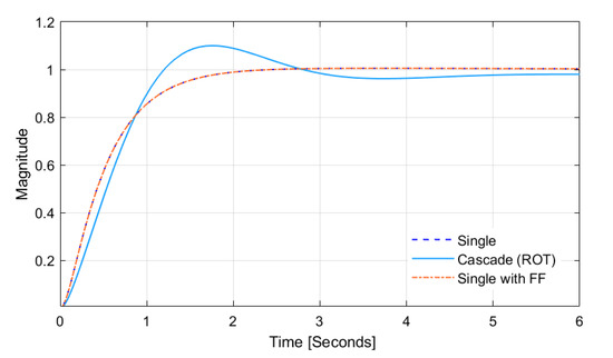
Figure 13.
Reference tracking results without a disturbance for a single controller and cascade controllers.
Figure 14 shows how the disturbance rejection was eliminated efficiently by a single controller, a single controller with feed-forward, and cascade controllers. The single PI controller showed good performance in the absence of a disturbance, but the settling time, overshoot, and reference tracking in the presence of a disturbance were poor.
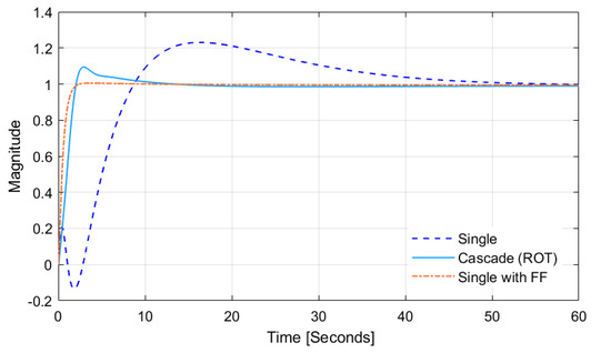
Figure 14.
Reference tracking results with a disturbance for a single controller and cascade controllers.
Table 6 provides specific figures on how effectively these controllers respond to disturbances. The cascade control system and PI control system with feed-forward perform better in rejecting a disturbance than the singe control system.
Table 6.
Performance results of a single PI controller, a single PI controller with feed-forward, and cascade controllers.
4.2. Comparison between a Single PI Controller with Feed-Forward, Cascade Controllers, and Combined Cascade/Feed-Forward Controllers
We directly compared the performance of a PI controller with feed-forward, cascade controllers, and combined cascade/feed forward controllers. The PI controller with feed-forward performed the same as in Section 4.1. Cascade controllers and combined cascade/feed-forward controllers were tuned by ROT, ZN, and TL. A feed-forward controller for combined cascade/feed-forward controllers was used with the same controller as a PI controller with feed-forward. In the case without a disturbance, cascade controllers and combined cascade/feed-forward controllers performed the same because the feed-forward controller does not work without a disturbance in the system. Table 7 shows the performance of each controller without a disturbance.
Table 7.
Performance results of a single proportional–integral (PI) controller with feed-forward, cascade controllers, and a combined cascade/feed forward controller without a disturbance.
Figure 15 depicts the performance when a disturbance was input to each controller. Combined cascade/feed-forward controllers showed relatively better performance when cascade controllers were not finely tuned. In the case of the combined cascade/feed-forward controllers tuned by ROT, IAE and ITAE increased compared to the without disturbance case, but the settling time was faster than the case without a disturbance. Unlike the combined cascade/feed-forward controllers, the cascade controllers have a longer settling time.
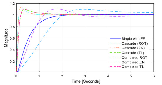
Figure 15.
Reference tracking results with a disturbance for a single controller with feed-forward (FF), cascade controllers, and combined cascade/FF controllers.
Well-tuned controllers, such as the ZN method and TL method, do not perform much differently between the cascade controller and the proposed method, but the combined cascade/FF controllers perform slightly better in IAE and ITAE with a rapid settling time when a disturbance was applied.
A PI controller with feed-forward showed good overall performance but performed poorly compared with the combined cascade/feed-forward controllers in settling time. For the combined cascade/feed-forward controller, settling time decreased from 6 to 5.6 s with a disturbance, but a PI controller with feed-forward remained at 1.9 s regardless of the disturbance. Combined cascade/feed-forward controllers using the TL method showed a fairly fast settling time of 0.65 s regardless of disturbance. Table 8 shows the performance of each controller with a disturbance.
Table 8.
Performance results of a single PI controller with feed-forward, cascade controllers, and a combined cascade/feed forward controller in case of with disturbance.
5. Discussion
As the objective of this study, we proposed a methane number adjustment system and combined cascade/feed-forward controllers to meet the methane number required by engine manufacturers and to ensure stable operation and robust performance of the methane number system. Regarding the control method of the methane number system, we obtained better performance than the existing methods by applying the tuning parameters used in the industry by combining two different controllers rather than focusing on tuning the controllers.
- (1)
- In terms of performance, if the methane number is lower than the engine requirements, LNG is supplied to the in-line mixer to condense C2+ which lowers the MN. This is effective at eliminating hydrocarbon, which lowers the methane number of the NG. When applying the MN system, the Otto-cycle engine is advantageous from the OPEX of view as it prevents the part being damaged by the knocking phenomenon [29]. The necessary information about the amount of LNG required in the MN system is obtained from the HYSYS dynamic simulation. Approximately 160 kg/h of the LNG is required on a simulation basis at the speed of 19 knots if the boil-off rate is 0.15% for LNG carriers (174,000 m3); however, it is a small amount considering the FG pump capacity of actual LNGC. This issue could be solved by controlling an appropriate amount of LNG to be supplied through a MN control system. In the normal case, stable control is possible even with a general controller, but when a large amount of LNG is suddenly supplied to the MN system due to a failure to control the discharge amount of the FG pump, a robust control system is needed.
- (2)
- For ensuring an MN adjustment system’s stable operation and robust control, combined cascade/feed-forward controllers were applied considering a disturbance occurrence. This proposed method can ensure that the IAE and ITAE values are smaller than the values of the other controllers examined in this study when a disturbance occurs, so the error could reduce, and the settling time is faster or the same. This proposed method is more effective for controller parameters used in industry in general than those tuned using the Ziegler–Nichols method and the Tyreus–Luyben method.
In future work, we will examine not only the contents in this study but also many fields of industry and compare performance through simulation and actual testing.
6. Patents
The patent for the mechanism of MN adjustment was registered at the Korean Intellectual Property Office on 20 November, 2018. Patent applicant is Daewoo Shipbuilding and Marine Engineering and patent developer is SoonKyu Hwang.
(Patent register number: 1019220300000, DOI: 10.8080/1020170144011)
Author Contributions
Conceptualization, S.H.; methodology, S.H.; software, S.K. Hwang; writing—original draft preparation, S.H.; writing—review and editing, S.H. and B.J.; supervision, S.H. and B.J. All authors have read and agreed to the published version of the manuscript.
Funding
This research received no external funding.
Conflicts of Interest
The authors declare no conflict of interest.
References
- YuanHang, H.; YunJia, L.; Xiao, L. Mixed aleatory/epistemic uncertainty analysis and optimization for minimum EEDI hull foam design. Ocean. Eng. 2019, 172, 308–315. [Google Scholar]
- Elizabeth, L.; Torstein, B. Potential power setups, fuels and hull designs capable of satisfying future EEDI requirements. Transp. Res. Part D 2018, 63, 276–290. [Google Scholar]
- Kim, A.R.; Seo, Y.J. The reduction of SOx emissions in the shipping industry: The case of Korea companies. Mar. Policy 2019, 100, 98–106. [Google Scholar] [CrossRef]
- Paul, G. From reductionism to systems thinking: How the shipping sector can address Sulphur regulation and tackle climate change. Mar. Policy 2014, 43, 376–378. [Google Scholar]
- Heather, T.; James, J.C.; James, J.W. Natural gas as a marine fuel. Energy Policy 2015, 87, 153–167. [Google Scholar]
- DongKyu, C.; HyunJun, S. A New Reliquefaction System of MRS-F (Methane Refrigeration System—Full Reliquefaction) for LNG Carriers; Gastech: Tokyo, Japan, 2017. [Google Scholar]
- WinGD. Available online: https://www.wingd.com/en/technology-innovation/engine-technology/x-df-dual-fuel-design/ (accessed on 19 April 2020).
- Partho, S.R.; Christopher, R.; SangKeun, D.; ChanSeung, P. Development of a natural gas Methane Number prediction model. Fuel 2019, 246, 204–211. [Google Scholar]
- Mario, M.; Rafael, D.H.; Vega, R. Comparison of evaporation rate and heat flow models for prediction of Liquefied Natural Gas (LNG) ageing during ship transportation. Fuel 2016, 177, 87–106. [Google Scholar]
- Martin, M.; Daniel, B.O. Methane number testing of alternative gaseous fuels. Fuel 2009, 88, 650–656. [Google Scholar]
- Wayne, B. Process. Control.: Modeling, Design, and Simulation, 1st ed.; Prentice Hall: Upper Saddle River, NJ, USA, 2003; pp. 313–332. [Google Scholar]
- YongHo, L.; MoonYong., L.; SunWon, P. PID controller tuning to obtain desired closed-loop responses for cascade control systems. Am. Chem. Soc. 1998, 37, 1859–1865. [Google Scholar]
- Ibrahim, K. Improving performance using cascade control and a Smith predictor. ISA Trans. 2001, 40, 223–234. [Google Scholar]
- Ibrahim, K.; Nusret, T.; Derek, P.A. Improved cascade control structure for enhanced performance. J. Process. Control. 2007, 17, 3–16. [Google Scholar]
- Wei, Z.; Hongbin, W.; Zhiming, Z.; Ning, L.; Pengheng, Y. Multilayer Feed-forward Neural Network Deep Learning Control with Hybrid Position and Virtual-force Algorithm for Mobile Robot Obstacle Avoidance. Int. J. Control. Syst. 2019, 17, 1007–1018. [Google Scholar]
- Manar, L.; Mohamed, F.; Abdelfatah, M.M.; Tomoyuki, M. Dynamic Modeling and Inverse Optimal PID with Feed-forward Control in H∞ Framework for a Novel 3D Pantograph Manipulator. Int. J. Control. Syst. 2018, 16, 39–54. [Google Scholar]
- IllWoo, P.; JinOh, K.; MyungHwan, O.; WooSung, Y. Realization of stabilization using feed-forward and feedback controller composition method for a mobile robot. Int. J. Control. Syst. 2015, 13, 1201–1211. [Google Scholar]
- Ehsan, A.; Ghazanfar, S. A new practical feed-forward cascade analyze for close loop identification of combustion control loop system through RANFIS and NARX. Appl. Therm. Eng. 2018, 133, 381–395. [Google Scholar]
- Nguyen, N.S.; Cao, V.K.; Ho, P.H.A. A novel adaptive feed-forward-PID controller of a SCARA parallel. Robot. Auton. Syst. 2017, 96, 65–80. [Google Scholar]
- YongHo, L.; Mikhail, S.; MoonYong, L. Analytical method of PID controller design for parallel cascade control. J. Process. Control. 2006, 16, 809–818. [Google Scholar]
- Philip, J.P. Introduction to Fluid Mechanics, 8th ed.; John Willey & Sons: Hoboken, NJ, USA, 2011; p. 391. [Google Scholar]
- The Spray Nozzle People. Available online: https://www.spray-nozzle.co.uk/spray-nozzles-by-industry/chemical-processing-old/gas-conditioning (accessed on 22 March 2020).
- GTT NO.96. Available online: https://www.gtt.fr/en/technologies/no96-systems (accessed on 22 March 2020).
- Lennart, L. System Identification-Theory for the User, 1st ed.; Prentice Hall: London, UK, 1987; pp. 13–66. [Google Scholar]
- Lennart, L. System Identification Toolbox-Getting Started Guide, 23rd ed.; The Mathworks: Natick, MA, USA, 2018; pp. 32–148. [Google Scholar]
- Karl, J.Å.; Björn, W. Adaptive Control., 2nd ed.; Prentice Hall: Upper Saddle River, NJ, USA, 1994; pp. 41–82. [Google Scholar]
- Emerson Fisher. Control. Valve Handbook, 5th ed.; Emerson Automation Solutions: Marshalltown, IA, USA, 2019; pp. 23–45. [Google Scholar]
- Jianhua, Z.; Fenfang, Z.; Mifeng, R.; Guolian, H.; Fang, F. Cascade control of superheated steam temperature with neuro-PID controller. Isa Trans. 2012, 51, 778–785. [Google Scholar]
- Zhi, W.; Hui, L.; Rolf, D.R. Knocking combustion in spark-ignition engines. Prog. Energy Combust. Sci. 2017, 61, 78–112. [Google Scholar]
© 2020 by the authors. Licensee MDPI, Basel, Switzerland. This article is an open access article distributed under the terms and conditions of the Creative Commons Attribution (CC BY) license (http://creativecommons.org/licenses/by/4.0/).