Abstract
The increase in global warming has secured the arctic region as a research hotspot, and the existence of ice floes and massive icebergs poses a great challenge to the navigational safety of polar ships. For the finite simulation of ship–ice collisions, a reasonable description of the ice constitutive model is the most important factor for the accuracy of ice load prediction and structural deformation assessment. Due to the complex physical properties of natural sea ice materials, there are still many difficulties in achieving a widely accepted ice material model. In this paper, a constitutive model of ice material considering the influence of temperature is established and embedded into finite element software LS-DYNA, and the material property parameters are validated and analyzed. Then, the drop test in a published paper is recapitulated by the numerical simulation with the proposed method, and the results are compared. Good agreement is attained between the numerical simulation and published results. The influences of temperature and drop height are discussed, and the results show that both of them have an important effect on structural deformation. The research results can be used for ice load prediction and polar ship structure design.
1. Introduction
The vast arctic waters are currently the largest area with undiscovered oil and gas reserves on earth, and the actual proven reserves are equivalent to 10% of the currently known petroleum resources [1]. Meanwhile, the sharp decline in sea ice caused by global warming presents the possibility of the full opening of the Arctic waterway, which will significantly shorten the trading distance between Asia and Europe by more than 3000 km, or one third of the current distance [2]. The risk of collision between ships and sea ice is greatly increased, which will cause not only irreparable life, property and economic losses but also catastrophic damage to the fragile polar ecosystem. Therefore, it is of great significance to study the collision performance between sea ice and ship structures. The constitutive model of sea ice is the most important aspect of such study, as it will significantly affect the accuracy and rationality of the calculation results.
Sea ice is a complex mixture composed of crystalline ice, brine, air and impurities, and its proportions vary with external conditions, time and space [3]. However, as a temperature-sensitive material, temperature, the basic thermal parameter, greatly influences the physical properties of sea ice both in its growing stage and existing stage. In early studies, researchers mostly studied the material properties of sea ice, including the physical and mechanical properties [4,5,6]. Then, empirical formulas were obtained from mechanical tests and used in the estimation of ice load levels under different collision scenarios [7,8,9,10], which is simple and effective, but the precision is low and the application scope is limited. In fact, the ice material is in a significant three-dimensional stress state during the ship-ice crushing process, similar to that of soil. With the development of testing technology, triaxial compression tests have been carried out, and the three-dimensional mechanical characteristics of sea ice are intuitively and comprehensively reflected, which provides effective data support for numerical simulations [11,12,13]. The test data show that the deformation of sea ice in nature presents a value of plasticity with a certain degree of random variability, but in practice, the average value is used as the plasticity parameter, especially in large-scale ice field calculations [14]. The thermodynamic-dynamic sea ice model based on the viscoplastic rheological theory proposed by Hibler [15] has been widely accepted as a classical sea ice dynamic model and was modified by Ji [16] to establish a model that can reasonably simulate the viscoelastic behavior of sea ice under small strain and strain rates of sea ice in the Bohai Sea area. In addition, hardened foam materials and other similar brittle materials have also been used in the simulation of sea ice materials [17,18], which is convenient and fast but cannot fully reflect the actual physical properties of ice. In recent years, based on reliable test data, user-defined constitutive subroutines have been developed and applied to ship-ice collision scenarios [19,20,21], which have been improved as a feasible and effective method. For ship-ice sheet collision scenarios, the cohesive segments method and smoothed particle hydrodynamics (SPH) method are also widely used [22,23,24], in which the DynaRICE model was the first software using SPH for river ice. However, due to the complexity of the ice properties, which is affected by regional and environmental factors, it is difficult to build a unified mathematical model to express it. Moreover, the ice properties are also sensitive to strain rate, temperature and the coexistence of multiple failure modes. So, there are still many difficulties to establish an accurate and comprehensive sea ice model considering all of the affected factors.
In this paper, the constitutive relationship of sea ice material is established. An elastic-plastic constitutive model with multisurface yield criterion and multiple empirical failure criterion is proposed. Moreover, the corresponding user-defined subroutine is developed and embedded in finite element software LS-DYNA. The influence of temperature is considered while the shear strength and the diversity of material properties that has little effect on the results for collision scenarios. Based on this, simulations and comparisons of drop test experiments of ice blocks conducted by a published paper are carried out, and the effects of temperature and drop height are discussed. The research results in this paper can be used for ice load prediction and polar ship structure design.
2. Ice Material Model
2.1. Ice Material Model Considering the Temperature Effects
For numerical simulations, uniaxial and triaxial experiments are the most important tests for the measurement of material parameters and are essential for the establishment of a sea ice constitutive model. Through uniaxial compression tests, some basic mechanical parameters of the ice can be obtained, which can be used in empirical formulas to describe ice loading; however, in the actual ship-ice interaction process, sea ice at the contact surface undergoes a more complex three-dimensional stress-strain relationship state before failure. A triaxial test can reveal the three-dimensional stress relationship of sea ice damage. Derradji-Aouat [25,26] gives a uniform multisurface yield criterion for isotropic fresh water ice, iceberg ice and columnar ice, as shown in formula (1), which is widely accepted and used.
The yield surface is an ellipse, is the ellipse center coordinate, is the octahedral stress, where , is the hydrostatic pressure, and and are the maximum octahedral stress and ultimate hydrostatic stress, respectively. Since , the above formula can be converted to
where is the second deviator invariant, which can be expressed in various ways, and in terms of the principal stress component, it is written as
Obviously, it is a modification of the von Mises’ yield criterion, and the form of the yield formula can be written in terms of parameters and J2 as
Writing the coefficient value in a more simplified form gives
where is the yield function, and the yield criterion is a form of the so-called Tsai-Wu yield criterion, which is suitable for describing materials with different tensile and compressive strengths, such as ice and soil, as shown in formula (6) in tensor notation [27].
where is stress tensor, , and means tensile and compression loading conditions, , , , , , , , , , , .
The yield criterion objectively reflects the fact that the hydrostatic pressure under complex stress conditions will affect the yielding state of the ice material. The material properties of sea ice vary with strain rate and temperature. According to the experiment [12,28], as shown in the yield curve at different temperatures in Figure 1, as the ship-iceberg collision involves high strain rates (larger than 10−3 s−1), the ice should be in a brittle failure mode, and the deformation of the sea ice before the plastic stage can be simply regarded as linear elastic behavior [19]. Therefore, the strain rate effect is not taken into consideration in this paper.
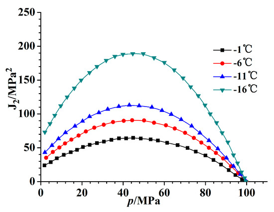
Figure 1.
Yield curve at different temperatures.
Considering the rationality of the constitutive model, an elastic-plastic constitutive model with brittle failure characteristics is established. The yield function parameters are fitted by MATLAB, and the yield formulas of ice materials at different temperatures are obtained. In a specific scenario, a0, a1, and a2 are constants, which are
For an elastic-plastic constitutive model, three issues must be considered: the plastic potential function for determining the direction of plastic strain, the yield function for judging the conditions for entering the yield state, and the coordination formula for calculating the magnitude of the plastic strain. The constitutive model satisfies the isotropic generalized Hooke’s law at the elastic stage, and its incremental form is
where is the hydrostatic strain increment, , and is the hydrostatic stress increment, . In the plastic phase, due to the convexity of the yield surface, the plastic strain increment can be written as
Using the associated flow rule in the plastic stage, is the yield function, and the above formula can be transformed to
where is the stress increment and is the Kronecker symbol, and its value is 0 () or 1 ().
In addition to the yield criterion, a reasonable failure criterion also needs to be established to simulate the damage characteristics of sea ice materials. There are many kinds of failure modes, and under normal circumstances, the damage forms of ice materials mainly include compression failure, tensile failure and shear failure. In dealing with ship-ice collision problems, the use of shear failure criteria actually underestimates the tensile strength or compressive strength of the ice material, causing the unit to failure prematurely. In actual situations, ice will also undergo a plastic stage during the extrusion process of ice, the hydrostatic stress of the ice material increases, and the strength increases significantly. Obviously, this compressive failure criterion is more difficult to satisfy. Considering that the upper limit should be used in practical applications, a dynamic failure strain criterion related to the rate-independent and cumulative plastic strain is used in this paper to define the failure of the element. The criterion originates from Jordaan’s empirical formula [29] and is used by Liu [19] and Gao [20], as shown in formula (10, 11)
where , , , and are constant parameters, and is a parameter related to the curve form. Similarly, this paper gives an improved empirical failure criterion, considering the temperature effect and adding the temperature term, that is:
When or , the element fails. Here, is the equivalent plastic strain, , is the failure strain, , and is the truncated stress. In addition, taking the tensile strength into consideration, the tensile strength limit is 2 MPa. is the initial failure strain and is set as the lowest point of the failure curve to 0.01. This failure criterion is characterized by focusing on the difference in the bearing capacity between the high stress zone and the low stress zone caused by the hydrostatic stress, the restraining friction slip, and the weakening effect of the shear failure in ship-ice collision problems.
2.2. Stress Update Algorithm
When updating the constitutive formula, the numerical algorithm is actually a stress update algorithm or constitutive integral algorithm. For rate-independent plasticity, the commonly used constitutive integral algorithm includes explicit algorithms, implicit algorithms and semi-implicit algorithms. A generalized rate-independent elastic-plastic constitutive model can be written as [30]
where , , and denote the total strain, elastic strain and plastic strain, is the Cauchy stress, represents the plastic variables, is the plastic flow direction, is the plastic parameter and is the plastic moduli.
Before the constitutive formula enters the plastic stage, the ice material is in an ideal elastic state, and the stress is calculated directly by Hooke’s law. While entering the plastic stage, in the next short time period t, the trial stress is obtained by Hooke’s law and is updated in the same way as in the elastic stage; if the stress exceeds the yield limit, it enters the iteration step. The nearest point projection method is used, which is a semi-implicit returning mapping algorithm, and the integral expression can be expressed as follows
where n is the iteration number, and are the strain and plastic strain in step n, is the strain increment, is the plastic increment parameter, and is the elastic matrix. It can be seen that an implicit algorithm is applied to the plasticity parameter , while an explicit algorithm is applied to the plastic flow direction and the plastic modulus . At the end of each step, the increment of the plasticity parameter is calculated, and the yield condition is strengthened. The plastic stage formula of the above equations is expressed as
Thereafter, the convergence condition is checked in each iteration step, and if it converges, the iteration is exited; otherwise:
The plastic strain increment is , and it can be put into formula (13) to obtain
In the formula, is the prediction stress and is the value of plastic correction. The specific steps are as shown in Figure 2, and the corresponding subroutine is generated after the program execution ends.
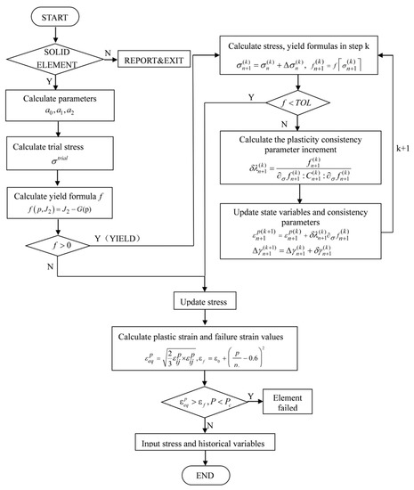
Figure 2.
Stress update algorithm flow.
2.3. Verification and Comparative Analysis of Sea Ice Materials
First, the single element test model is established, and the compression and tensile loads are applied separately. In the subroutine calculations, to verify the logical correctness of the related parameters, the values of the second deviating stress invariant (), the hydrostatic stress () and the failure strain () are outputted, and the curves obtained are shown in Figure 3, Figure 4 and Figure 5, respectively.
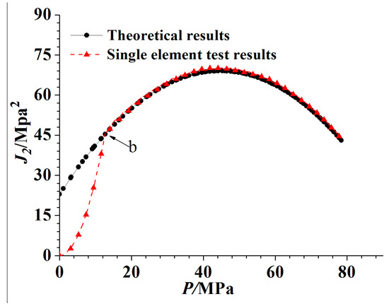
Figure 3.
Comparison of relationship between theoretical results and single element test results.
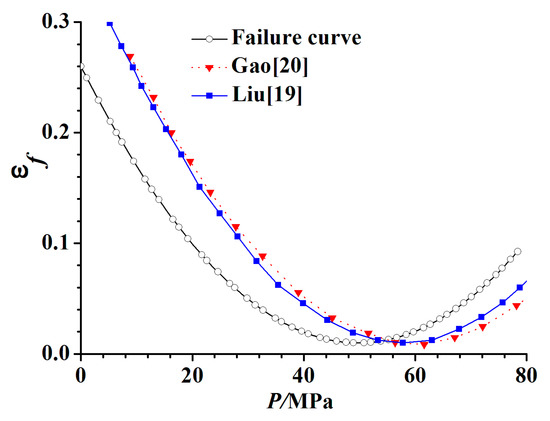
Figure 4.
Comparison of curves obtained from single element test and other researchers.
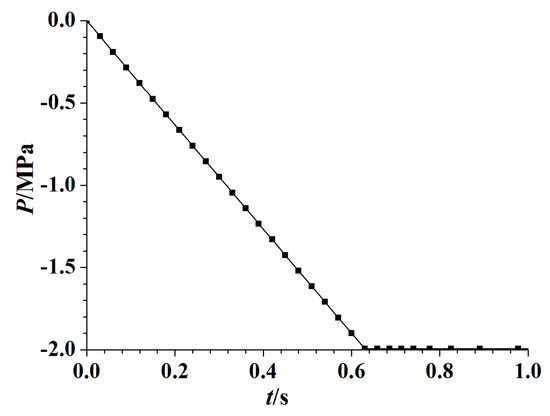
Figure 5.
Relationship obtained from single element test.
From Figure 3, it can be seen that the second invariant of the deviatoric stress has a quadratic relationship with the hydrostatic stress. The theoretical curve is a standard curve (black), and before point b, the output value is lower than the theoretical value, indicating that the element is in the elastic stage. When point b is reached and exceeded, the two lines coincide, and the element reaches the yield state. The initial yield point is approximately 10 MPa, which is in line with the theoretical solution. At the same time, the failure strain curve is also quadratic with hydrostatic stress, and its minimum value is 0.01, which is consistent with the set theoretical value and tend to be more likely to fail than Liu’s and Gao’s model [19,20]. Under tensile loading, the minimum hydrostatic stress is −2 MPa and is the same as the theoretical tensile ultimate strength, namely, the truncation stress, which shows that the subroutine algorithm is convergent and correct.
Then, a rigid plate-spherical ice crushing model is established, and the rationality of the material is verified by the pressure-area curve. The diameter of the ice sphere is 1 m, and the side length of the rigid plate is 3 m. The side of the rigid plate is fixed and impacted by the ice sphere at a constant speed of 1 m/s. The deformation of the ice sphere at 0.5 s is shown in Figure 6. It can be seen that the surface of the ice sphere has been damaged, the failure surface is jagged, there are visible but small amounts of ice blocks falling off, and the stress distribution on the contact surface is uneven. The high stress areas and low stress areas are obvious. The maximum stress is approximately 23.5 MPa, and the minimum stress is approximately 2 MPa, which indicates that the strength of the material is enhanced under three-dimensional compressive stress.
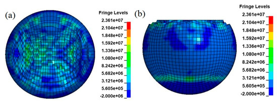
Figure 6.
Damage of the ice ball at 0.5 s. (a) Main view (b) Side view.
The collision force and pressure-area curve are shown in Figure 7 and Figure 8, respectively. The collision force shows typical nonlinear characteristics due to instantaneous element failure. The force value increases significantly at the beginning of the crushing process due to the rapid increase in the contact area, and then the increase is gradual. Figure 8 shows the comparison of the pressure-area curves calculated during the process with ISO standards and those measured by other researchers. It is shown that the general trend of the pressure-area curve is in good agreement with the ISO standard and the results of other researchers. While the contact area is small in the beginning, the value is close to the standard value, and is significantly larger than the results of Timco’s and Molikpad Design’s [31], as the area increases, the average pressure value gradually decreases and approaches the standard value, the pressure value tends to be flat at the end, and the consistency with the standard curve is good. It should be noted that the pressure-area curve of the ISO standard is based on the limit state design (ULS) and the accidental limit state (ALS) method, which means that the pressure measurement takes the limit value, makes the value slightly smaller than the standard value. By contrast, the pressure-area curve obtained in this paper is more consistent with the curve obtained by other researchers when the contact area is large, and reduces the deviation of their values from the ISO curve when the area is small, makes it more reasonable.
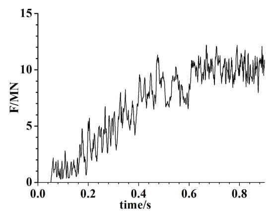
Figure 7.
Force-time curve of the collision model between ice sphere and rigid plate.
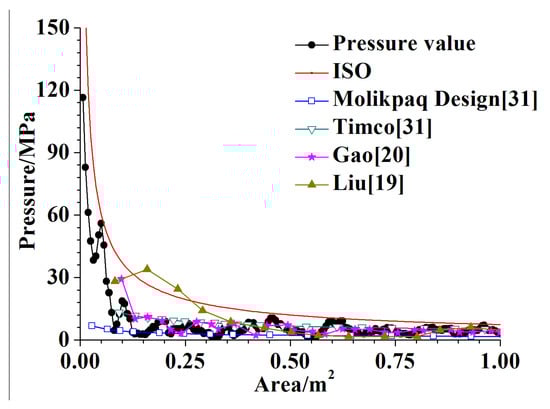
Figure 8.
Comparison of pressure-area relationship between this study and other researchers.
To study the characteristics of the high stress zone and low stress zone during the reaction process, Figure 9 and Figure 10 show the positions of the nodes that are located diagonally in a partial area (1.0 m × 1.0 m) of the rigid plate and the nodal force of each node at four time points, 0.2 s, 0.4 s, 0.6 s and 0.8 s. It can be seen that as the crushing failure progresses, there exists a mutual transformation between the high-pressure zone and low-pressure zone. The closer the node is to the center, the greater the variation range of the node force is, and it gradually decreases from the center to the periphery.
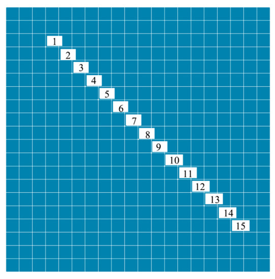
Figure 9.
Node location on rigid plate.
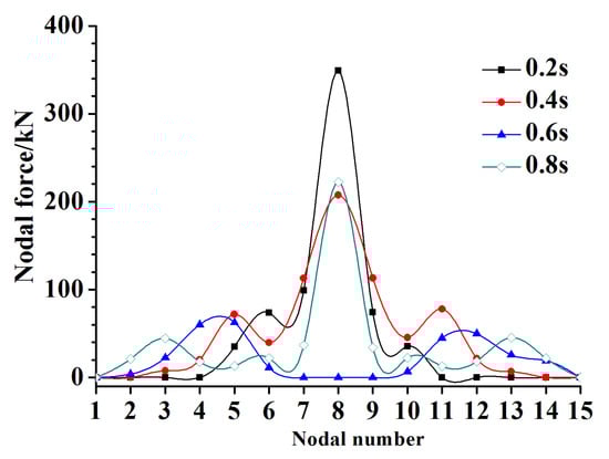
Figure 10.
Nodal force at different times.
Figure 11 and Figure 12 are curves of the failure stress and strain of the single element under continuous compression loading at different temperatures. It can be seen that with the decrease in temperature, the failure stress increases, indicating that the material becomes stronger, while the failure strain decreases, indicating that the material becomes brittle, which is in good agreement with the experimental conclusions. The pressure-area curves at different temperatures are shown in Figure 13. It can be seen that the pressure-area curves at different temperatures have the same trend, which is smaller than the ISO standard curve at the beginning and is consistent with the standard curves when the pressure tends to stabilize. The pressure value at lower temperatures is slightly higher, and the differences are not obvious, which shows that the yield criterion plays a more important role in the influence of temperature on the material properties.
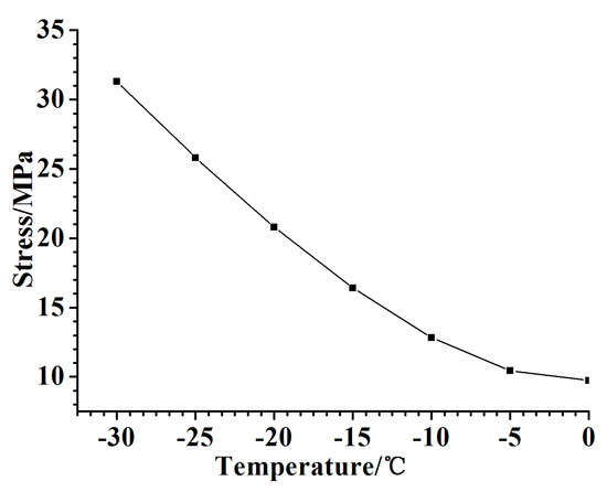
Figure 11.
Failure stress-temperature curve.
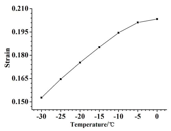
Figure 12.
Failure strain-temperature curve.
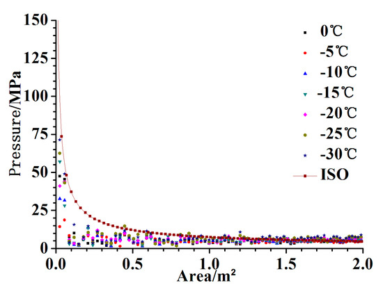
Figure 13.
Pressure-area curves at different temperatures.
From the figures above, it can be seen that, compared to natural sea ice materials, the user-defined ice material proposed in this paper produces a fairly accurate simulation of the ice load and the deformation characteristics under compressive loads, reasonably reflecting its temperature sensitivity characteristics.
3. Numerical Simulation Analysis of the Ice Drop Test
3.1. Experimental Introduction
In 2013, Kim [32] conducted a series of drop impact tests on ice blocks and stiffened plate frames at Norwegian University of Science and Technology and Aalto University, as shown in Figure 14. In this section, a typical condition with a drop height of 3.0 m will be selected and compared.

Figure 14.
Photographs of the drop test experiment.
The typical stiffened plate frame structure in the test is shown in Figure 15. The size of the stiffened plate frame is 1.1 m by 1.1 m, the spacing between the stiffeners is 150 mm, and the spacing between the ribs is 500 mm. There are L-shaped support plates on both sides to provide a rigid boundary. According to the plate thickness difference of each structure, the plate frame is divided into three types. In this paper, the P3 plate is used, as shown in Table 1.
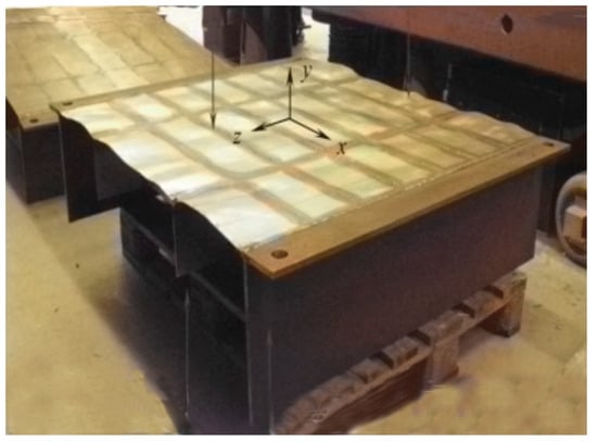
Figure 15.
Photographs of the stiffened panel.

Table 1.
Thickness of the stiffened plate.
The test was carried out at a temperature of 3°C. The ice samples consisted of laboratory ice, and the density was 900 kg/m3. The stiffened plate was made of S235 steel, and the engineering stress-strain curve is shown in Figure 16. The ice block was used as the object of the free-fall drop impact, the maximum length and depth of the dent were measured, and the crushing process was recorded by a high-speed camera.
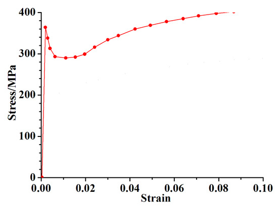
Figure 16.
Engineering stress-strain curve of mild steel.
3.2. Finite Element Model
The computations are implemented by LS-DYNA. The finite element model is shown in Figure 17. The dimensions of the plate frame and the ice block are exactly the same as the test, the plate frame is modeled by four-nodes and five-integration-point shell elements (thin shell 163), and the ice block is modeled by solid elements (solid 164). Both ends parallel to the rib of the plate are rigidly fixed, while the ice block has no constraints during the simulation. In addition, a 5.0 mm overall finite element length was developed for the stiffened plate, and the size of the ice block was the same.
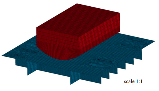
Figure 17.
Finite element model of the drop test.
In the simulation, the initial fall height of the ice block is converted to the initial velocity to reduce the calculation time, which is 3 m and 7.67 m/s2, and the temperature of the ice block is set to −5 °C as a result of comprehensive consideration of the ice block reserving temperature and the room temperature. A “combined material” [33,34,35] is used for the direct simulation input of the steel material, and the temperature of the stiffened plate is not considered. Furthermore, the drop test experiment is a strong, nonlinear high strain rate problem, so the hardening phenomenon and strain rate effect of the material cannot be ignored. In this paper, using the Cowper-Symonds constitutive formula [36], the materials D and P of the low-carbon steel are 40.4 and 5, respectively.
3.3. Numerical Results
Figure 18 and Figure 19 show the deformations of the stiffened plate from the simulation. It can be seen that due to the relatively weak material strength of the sea ice and the failure during collision, the deformation is concentrated in the central contact position and presents a continuous concave deformation because of the existence of the stiffener. The maximum stress reaches 385 MPa and the maximum strain is nearly 0.03, which shows that the effect of the strain rate is obvious, and the deformation length is approximately 750 mm between the 5 stiffened plates, which is consistent with the test results.
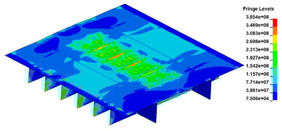
Figure 18.
Stress contours of the stiffened plate.
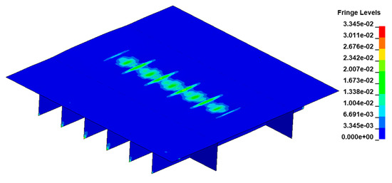
Figure 19.
Plastic strain contours of the stiffened plate.
The impact depth of the stiffened plate in the simulation is shown in Figure 20 and is compared with the experimental results [32]. Take the original plane as the datum plane, negative number represents depression, positive number represents unwarping, the collision depth results are basically the same. In the test, due to the low accuracy of the value measured, the maximum depth in the test is approximately 8 mm, and the contour is composed of broken lines, which is inclined to the right side of the plate frame, showing that the ice block is skewed to some extent during the falling process. In the simulation, the contours are curves because the height is converted into velocity, and the initial interval is very close, so the symmetry of the structure deformation is obvious, and the maximum depth is 8.6 mm. Considering that there is no loss of kinetic energy caused by the ice falling and due to the difficulty in accurately modeling the occurrence of cracks and ice splits in the simulation, it can be said that the plate deformation results in the simulation are conservative but reasonable.
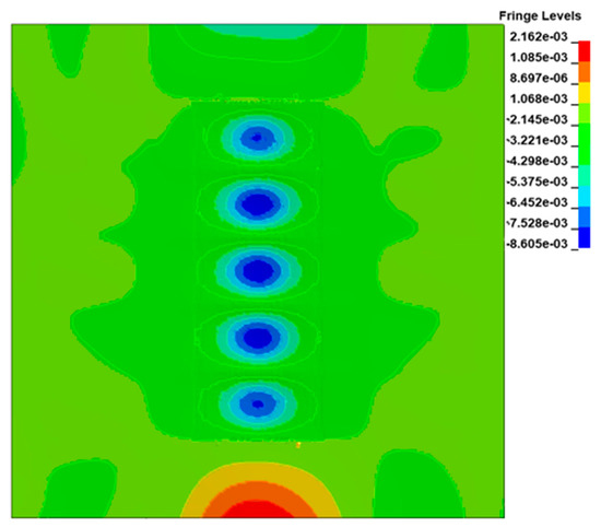
Figure 20.
Dent distribution in the simulation (m).
During the collision process, both the structure and the ice can undergo significant deformations. Figure 21 shows the damage and deformation of the ice block in the simulation. It can be seen that the ice block is mainly damaged in the form of element failure, the debris is minimal, the stress distribution is obviously localized, and the maximum stress is 8.9 MPa. In the experiment, the ice block is deformed and crushed irregularly during the test, with the generation of new splitting cracks and the extruded ice falling off. Therefore, for the deformation of ice material, because the finite element software is based on the continuum medium theory, user-defined ice material has limitations compared with actual ice material. Generally, the simulation results tend to be conservative.
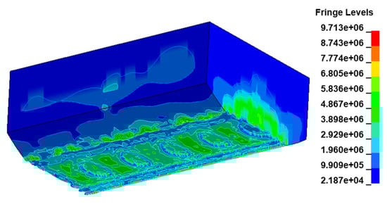
Figure 21.
Stress contours of ice block in the simulation.
Numerical analyses can offer much detailed information, and it is possible to record the data that are difficult to obtain in the test through simulation to understand the characteristics of the interaction between the plate frame and the ice block, such as the collision force and energy, which are shown in Figure 22, Figure 23 and Figure 24. Figure 22 shows the curve of the collision force during the drop test process. The entire dropping process time is approximately 0.14 s, and the impact force is typically nonlinear with multiple peaks, which are at 753.48 kN, 668.29 kN, and 540.31 kN, and gradually decrease with time.
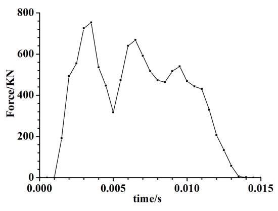
Figure 22.
Collision force-time relationship of the stiffened plate obtained from simulation.
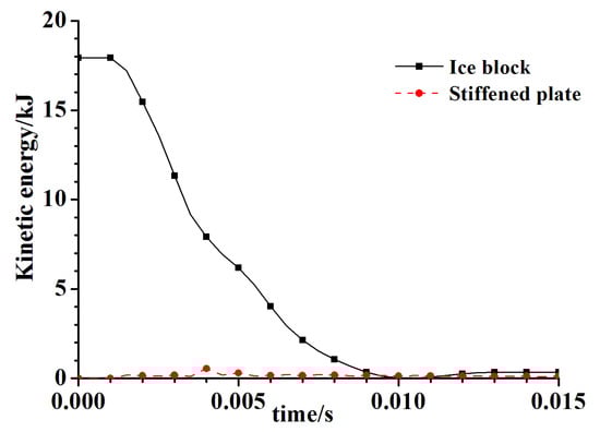
Figure 23.
Kinetic energy of the stiffened plate and ice block obtained from simulation.
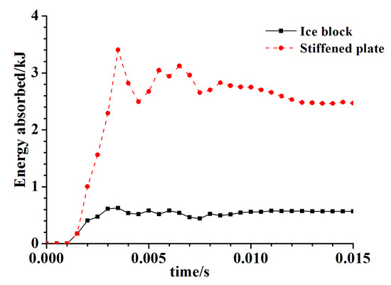
Figure 24.
Internal energy of the stiffened plate and ice block obtained from simulation.
Figure 23 and Figure 24 show the curves of the kinetic energy and internal energy of the ice block and stiffened plate. It can be seen that the kinetic energy of the ice block decreases rapidly during the collision process, the energy of the plate and the ice block is kept at a very small value, the energy absorbed by the ice block is approximately 0.5 kJ, and the internal energy of the structure is approximately 2.31 kJ, which is mostly due to the slightly larger deformation and the hard fragmentation of the ice block. The stiffened plate frame absorbs most of the energy.
The comparison between the simulation and test is summarized and shown in Table 2. It can be noted that in the test, the energy absorbed by the plate frame is smaller than that in the simulation, which is partly due to the calculation method of applying a uniform pressure until the deformation of the plate frame is equal to the measured value, and because the dynamic effect is not considered and there is a relatively large deformation. Additionally, considerable kinetic energy has also been lost due to ice fragmentation, which is the main reason for the energy error.
Table 2.
Comparison between the simulation and test.
Generally, under the comparison with the drop experiment, the user-defined ice material proposed in this paper can reasonably simulate the ice load and the basic deformation characteristics, and the error is within an acceptable range. While for the description of the ice damage and failure, especially its splitting and falling off, has limitations, which are mainly caused by the inherent characteristics of finite element theory, the simulation results are conservative, but still reasonable, and do not overestimate the strength of sea ice.
4. Discussions
4.1. Effect on the Temperature of the Ice Block
As a temperature-sensitive material, the properties of sea ice materials are dependent on temperature. In Section 2.3, we determined that the effect of temperature on a single element is significant but is not obvious in the pressure-area curve. However, for the deformable plate frame structure, it is necessary to study the change in the deformation of the plate frame under different temperature drop conditions.
Four different temperature scenarios, namely, −5°C, −10°C, −15°C, and −20°C, are modeled and calculated; the temperature effect of the plate frame is not considered, and other parameters remain unchanged in each scenario.
The deformation of the central section of the plate frame and the maximum depth are shown in Figure 25, in which five pits were marked as no. 1 to no. 5 from left to right. It can be seen that under different temperatures, the deformation shape of the middle sections of the stiffened plate is basically the same, the nodal displacement at the center of the plate frame is slightly larger than that at other locations along the plate frame. As the temperature of the ice decreases, the depth of each pit increases slightly, and the decreasing trend is approximately linear for the three pits in the central position, while linear characteristics are not obvious for the pits at the edge.
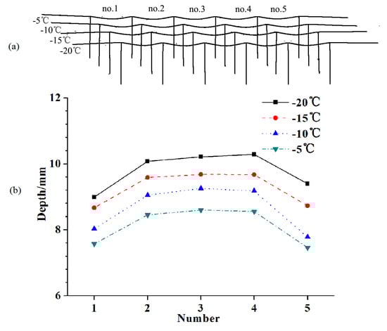
Figure 25.
Deformation and maximum depth at different temperatures. (a) Deformation of the middle sections of the plate frame. (b) Maximum depth measured in simulation.
The initial kinetic energy is the same as that of the typical scenario, which is 17.7 kJ. Table 3 shows the dent length, peak force and energy absorbed in the final state under different temperatures. It can be seen that, in general, as the temperature decreases, the peak force and the internal energy of the stiffened plate increase, which is in line with the previous conclusion that as the temperature decreases, the ice material gradually becomes harder and more brittle. The dent length remains unchanged, and the internal energy of the ice block also remains stable, generally, which indicates that the energy absorbed by the ice block is mainly related to its own deformation, while the temperature mainly affects the initial internal energy of sea ice. Of course, for extremely low temperatures, due to the lack of experimental data support, the applicability of the user-defined material cannot be guaranteed.
Table 3.
Variation in drop parameters at different temperatures.
4.2. Effect of the Drop Height of the Ice Block
Another factor that requires attention and has a greater influence on structural safety during polar voyages is the relative speed. Although Kim also performed drop tests at 1.1 m and 1.6 m, the results do not contribute to the analysis of the influence of the relative speed of a collision. In this section, five drop height simulation scenarios are established and analyzed, namely, 1 m, 1.5 m, 2 m, 2.5 m, and 3 m, which will be transformed into the velocity in the simulation.
Similarly, Figure 26 shows the deformation of the central section of the plate frame and the maximum depth of five pits marked as no. 1 to no. 5. It can be seen that the influence of the drop height on the deformation of the plate frame is significant, the deformation amplitude of the stiffened plate frame becomes increasingly obvious with the increase in the drop height, the relationship between the drop height and deformation amplitude is nonlinear, and as the height steadily increases, the increasing value of the deformation depth decreases gradually. At the same time, the situation in which the deformation of the middle part is larger than that of the two ends is not changed.
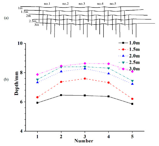
Figure 26.
Deformation and maximum depth at different drop heights. (a) Deformation of the middle section of the plate frame. (b) Maximum depth measured in simulation.
The kinetic energy has a linear relationship with the height at different drop heights, while the velocity does not, as shown in Table 4, which also shows the other parameters of the drop test. It can be seen that the dent length and energy absorbed by the ice block have no obvious change, and the energy absorbed by the ice block is maintained at approximately 0.5–0.6 kJ. This is because with the increase in the initial height, the energy absorption of the ice block increases, while the failure number of the ice elements also increases rapidly, which produces a trend of the energy absorption of sea ice that is not obvious. While the energy absorbed by the stiffened plate structure and the peak force increase rapidly with increasing height and have a nonlinear relationship with height, the general trend is similar to that of the deformation depth.
Table 4.
Variation in drop parameters at different drop heights.
5. Conclusions
In this paper, an ice material constitutive model considering the influence of temperature is proposed, and the corresponding LS-DYNA material subroutine is established. The ice material constitutive model proposed in this paper can effectively simulate the ice load under collision and correctly reflect the three-dimensional compressive strength characteristics of ice materials. The pressure-area curve is consistent with the ISO standard and other experimental results. The temperature has a direct effect on the material properties; as the temperature decreases, the material becomes harder and more brittle.
Through the simulation of the drop test, collision parameters such as the deformation and collision depth are compared. The results show that the simulation results are in good agreement with the test results, the error of the maximum depth is within the acceptable range, and the ice load can be relatively accurately obtained. However, for simulating ice damage and failure, especially the phenomena of ice splitting and falling off, the finite element method still has its limitations, which are mainly due to its inherent characteristics of the continuum theory.
Through the parameter sensitivity analysis of the drop test, the results show that temperature and drop height have an important influence on the deformation and damage of the stiffened plate. Relatively speaking, the influence of the temperature is less than that of the drop height change; at the same time, the influence of the temperature shows the characteristics of an approximately linearity relationship, while the effect of the drop height on the deformation of the plate is gradually reduced, which needs to be further verified by experiments.
In summary, compared with the experimental results and the research results of the sensitivity to the influence of the parameters, it is shown that the simulation results are consistent with the experimental deformation; generally speaking, the simulation results are more conservative without being too conservative. The ice material model proposed in this paper can be used for the analysis of actual ship–ice interaction scenarios.
Author Contributions
Conceptualization, T.Y., K.L. and Z.W.; methodology, T.Y.; software, T.Y.; validation, K.L., J.W. and Z.W.; formal analysis, T.Y.; investigation, T.Y.; data curation, K.L.; writing—original draft preparation, T.Y.; writing—review and editing, K.L. and Z.W.; supervision, K.L. and Z.W.; project administration, K.L. and Z.W.; funding acquisition, Z.W. All authors have read and agreed to the published version of the manuscript.
Funding
This research was funded by National Natural Science Foundation of China, grant number 51609110; 51779110; 51809122 and Six talent peaks project in Jiangsu Province, grant number KTHY-064.
Acknowledgments
We gratefully acknowledge the financial support of the National Natural Science Foundation of China (Grant No. 51609110; Grant 51779110; Grant 51809122) and Six talent peaks project in Jiangsu Province (Grant No.KTHY-064).
Conflicts of Interest
The authors declare no conflict of interest. The funders had a role in the decision to publish the results.
References
- Bird, K.J.; Charpentier, R.R.; Gautier, D.L.; Houseknecht, D.W.; Klett, T.R.; Pitman, J.K.; Moore, T.E.; Schenk, C.J.; Tennyson, M.E.; Wandrey, C.J. Circum-Arctic resource appraisal: Estimates of undiscovered oil and gas north of the Arctic Circle. In US Geological Survey Fact Sheet FS-2008-3049; USGS: Washington DC, USA, 2008; Available online: http://pubs.usgs.gov/fs/2008/3049/ (accessed on 5 May 2016).
- Suppiah, C.R. The Northeast Arctic Passage: Possibilities and economic considerations. Marit. Stud. 2006, 2006, 12–15. [Google Scholar] [CrossRef]
- Schwarz, J.; Weeks, W.F. Engineering properties of sea ice. J. Glaciol. 1977, 19, 499–531. [Google Scholar] [CrossRef][Green Version]
- Timco, G.W.; Frederking, R.M.W. A review of sea ice density. Cold Reg. Sci. Technol. 1996, 24, 1–6. [Google Scholar] [CrossRef]
- Hutchings, J.K.; Heil, P.; Lecomte, O.; Stevens, R.; Steer, A.; Lieser, J.L. Comparing methods of measuring sea-ice density in the East Antarctic. Ann. Glaciol. 2015, 56, 77–82. [Google Scholar] [CrossRef]
- Forsström, S.; Gerland, S.; Pedersen, C.A. Thickness and density of snow-covered sea ice and hydrostatic equilibrium assumption from in situ measurements in Fram Strait, the Barents Sea and the Svalbard coast. Ann. Glaciol. 2011, 52, 261–270. [Google Scholar] [CrossRef]
- Sodhi, D.S.; Haehnel, R.B. Crushing ice forces on structures. J. Cold Reg. Eng. 2003, 17, 153–170. [Google Scholar] [CrossRef]
- Dempsey, J.P.; Adamson, R.M.; Mulmule, S.V. Large-scale in-situ fracture of ice. In Proceedings of the FRAMCOS, Zurich, Switzerland, 25–28 July 1995; pp. 675–684. [Google Scholar]
- Dempsey, J.P., Shen, H.H., Eds.; IUTAM Symposium on Scaling Laws in Ice Mechanics and Ice Dynamics. In Proceedings of the IUTAM Symposium, Fairbanks, Alaska, USA, 13–16 June 2000; Volume 94, pp. 43–54. [Google Scholar]
- Daley, C.G. Energy based ice collision forces. In Proceedings of the 15th International Conference on Port and Ocean Engineering under Arctic Conditions (POAC), Espoo, Finland, 23–27 August 1999; Volume 2, pp. 674–686. [Google Scholar]
- Richter-Menge, J.A. Triaxial Testing of First-Year Sea Ice; US Army Corps of Engineers, Cold Regions Research & Engineering Laboratory: Hanover, NH, USA, 1986. [Google Scholar]
- Gagnon, R.E.; Gammon, P.H. Triaxial experiments on iceberg and glacier ice. J. Glaciol. 1995, 41, 528–540. [Google Scholar] [CrossRef]
- Cox, G.F.N.; Richter-Menge, J.A. Triaxial compression testing of ice. In Proceedings of the Civil Engineering in the Arctic Offshore. ASCE, San Francisco, CA, USA, 25–27 March 1985; pp. 476–488. [Google Scholar]
- Hibler, W.D. A viscous sea ice law as a stochastic average of plasticity. J. Geophys. Res. Atmos. 1977, 82, 3932–3938. [Google Scholar] [CrossRef]
- Hibler, W.D. A Dynamic Thermodynamic Sea Ice Model. J. Phys. Oceanogr. 1979, 9, 815–846. [Google Scholar] [CrossRef]
- Ji, S.; Shen, H.T.; Wang, Z.; Shen, H.H.; Yue, Q. A viscoelastic-plastic constitutive model with Mohr-Coulomb yielding criterion for sea ice dynamics. Acta Oceanol. Sin. 2005, 24, 54–65. [Google Scholar]
- Gagnon, R.E. A numerical model of ice crushing using a foam analogue. Cold Reg. Sci. Technol. 2011, 65, 335–350. [Google Scholar] [CrossRef]
- Kim, H. Simulation of Compressive ‘Cone-Shaped’ Ice Specimen Experiments using LS-DYNA. In Proceedings of the International Ls-Dyna Users Conference, Detroit, MI, USA, 8–10 June 2014. [Google Scholar]
- Liu, Z.; Amdahl, J.; Løset, S. Plasticity based material modelling of ice and its application to ship–iceberg impacts. Cold Reg. Sci. Technol. 2011, 65, 326–334. [Google Scholar] [CrossRef]
- Gao, Y.; Hu, Z.; Ringsberg, J.W.; Wang, J. An elastic–plastic ice material model for ship-iceberg collision simulations. Ocean Eng. 2015, 102, 27–39. [Google Scholar] [CrossRef]
- Shi, C.; Hu, Z.; Ringsberg, J.; Luo, Y. A nonlinear viscoelastic iceberg material model and its numerical validation. Proc. Inst. Mech. Eng. Part M J. Eng. Marit. Environ. 2017, 231, 675–689. [Google Scholar] [CrossRef]
- Wang, F.; Zou, Z.J.; Zhou, L.; Ren, Y.Z.; Wang, S.Q. A simulation study on the interaction between sloping marine structure and level ice based on cohesive element model. Cold Reg. Sci. Technol. 2018, 149, 1–15. [Google Scholar] [CrossRef]
- Lu, W.; Lubbad, R.; Løset, S. Simulating ice-sloping structure interactions with the cohesive element method. J. Offshore Mech. Arct. Eng. 2014, 136, 031501. [Google Scholar] [CrossRef]
- Kolerski, T.; Zima, P.; Szydłowski, M. Mathematical Modeling of Ice Thrusting on the Shore of the Vistula Lagoon (Baltic Sea) and the Proposed Artificial Island. Water 2019, 11, 2297. [Google Scholar] [CrossRef]
- Derradji, A. A unified failure envelope for isotropic fresh water ice and iceberg ice. In Proceedings of the ETCE/OMAE-2000 Joint Conference Energy for the New Millenium, New Orleans, LA, USA, 14–17 February 2000; Available online: https://core.ac.uk/display/38594362 (accessed on 30 December 2000).
- Derradji-Aouat, A. Multi-surface failure criterion for saline ice in the brittle regime. Cold Reg. Sci. Technol. 2003, 36, 47–70. [Google Scholar] [CrossRef]
- Clouston, P.; Lam, F.; Barrett, J.D. Incorporating size effects in the Tsai-Wu strength theory for Douglas-fir laminated veneer. Wood Sci. Technol. 1998, 32, 215–226. [Google Scholar] [CrossRef]
- Shi, C.; Hu, Z.; Ringsberg, J.; Luo, Y. Validation of a temperature-gradient-dependent elastic-plastic material model of ice with finite element simulations. Cold Reg. Sci. Technol. 2017, 133, 15–25. [Google Scholar] [CrossRef]
- Jordaan, I.J.; Matskevitch, D.G.; Meglis, I.L. Disintegration of ice under fast compressive loading. Int. J. Fract. 1999, 97, 279–300. [Google Scholar] [CrossRef]
- Ortiz, M.; Simo, J.C. An analysis of a new class of integration algorithms for elastoplastic constitutive relations. Int. J. Numer. Methods Eng. 1986, 23, 353–366. [Google Scholar] [CrossRef]
- Timco, G.; Sudom, D. Revisiting the Sanderson pressure–area curve: Defining parameters that influence ice pressure. Cold Reg. Sci. Technol. 2013, 95, 53–66. [Google Scholar] [CrossRef]
- Kim, E.; Storheim, M.; Amdahl, J.; Løset, S.; Von Bock und Polach, R.U.F. Drop tests of ice blocks on stiffened panels with different structural flexibility. In Collision and Grounding of Ships and Offshore Structures; Taylor & Francis Group: Milton Park, UK, 2013; pp. 241–250. [Google Scholar]
- Villavicencio, R.; Soares, C.G. Numerical plastic response and failure of a pre-notched transversely impacted beam. Ships Offshore Struct. 2012, 7, 417–429. [Google Scholar] [CrossRef]
- Dieter, G.E. Mechanical behavior under tensile and compressive loads. ASM Handb. 2000, 8, 99–108. [Google Scholar]
- Zhang, L.; Egge, E.D.; Bruhns, H. Approval procedure concept for alternative arrangements. In Proceedings of the 3rd International Conference on Collision and Grounding of Ships (ICCGS), Izu, Japan, 25–27 October 2004; pp. 87–96. [Google Scholar]
- Samuelides, E.; Frieze, P.A. Fluid-structure interaction in ship collisions. Mar. Struct. 1989, 2, 65–88. [Google Scholar] [CrossRef]
© 2020 by the authors. Licensee MDPI, Basel, Switzerland. This article is an open access article distributed under the terms and conditions of the Creative Commons Attribution (CC BY) license (http://creativecommons.org/licenses/by/4.0/).