Abstract
The present study describes a model-based approach for the assessment of central cooling retrofit solutions using variable speed drive (VSD) seawater (SW) pumps in marine applications. There are two main innovative features of the proposed methodology. The effect of boundary conditions (fluid stream temperatures and mass flow rates) on the performance of central SW/fresh water (FW) cooler is considered via a detailed heat exchanger simulation model. Additionally, the repercussion of the higher FW temperature on the main engine fuel consumption due to the incorporation of a VSD SW pump is examined. The proposed methodology is applied on a handy-size bulk carrier equipped with a shell and tube SW/FW central cooler and a two-stroke main diesel engine. Both the reduced power demand for the VSD pump and the increased brake specific fuel consumption (bsfc) of the main engine due to the increased low temperature (LT)/FW temperature have been considered at each operating point examined. Predictions have shown that in all part-load operating cases examined the use of a VSD SW pump has a positive effect on the reduction of total fuel consumption, whereas at full engine load, there is a SW threshold temperature under which the operation with a VSD pump leads to slightly higher total fuel consumption. This study highlights the importance of using an integrated approach for the reliable assessment of central cooling retrofit solutions, which can lead to optimized control solutions of the VSD pump operation for maximizing a ship’s fuel savings.
1. Introduction
Awareness of energy efficiency in the maritime sector has become of vital importance over the last decade [1], supported by strict international environmental legislation adopted by the International Marine Organization (IMO) and the continuous effort of the shipping industry to reduce its exposure to fuel price fluctuations and maximize the economic profits [2]. Specifically, IMO has correlated the reduction of greenhouse gas (GHG) emissions with the significant improvement of new and existing ships, and for this reason has issued the Energy Efficiency Design Index (EEDI), which is mandatory for new ships, and the Ship Energy Efficiency Management Plan (SEEMP) for all ships since the MEPC 62 on July 2011 [2]. The measures proposed in the literature up to now [3] have been split into three categories: technological, operational and market-based measures. Most of the technological energy efficiency improvement measures are based on the reduction of fuel consumption of the marine engines used for propulsion and electric power generation considering various solutions such as the use of alternative gaseous fuels [4] and optimized engine–propeller operational matching [5]. However, until recently, less energy demanding auxiliary systems such as cooling pumps have not been examined thoroughly. The situation is even worse in vessels with older designs, where the energy efficiency of auxiliary systems has not been considered during the design and construction phase [2]. Typically, the technical specifications of the auxiliary systems (such as pumps, fans, etc.) are chosen based on preliminary calculations of the required capacity, and after being installed their operation is not optimized based on the actual requirements of the system served [6]. This practice influences not only the energy efficiency of the system but seriously affects reliability, since usually these systems operate at off-design conditions for long periods [6].
Among the most energy demanding auxiliary systems installed on a vessel, which operate almost continuously under variable conditions, is the seawater cooling pump. It is mandatory (based on the international regulations [7]) that SW pumps should be able to cover the maximum heat load of the cooling system under extreme (i.e., tropical) environmental conditions. This is a situation which rarely occurs in every-day operations. Therefore, a SW pump chosen to fulfill this requirement would operate most of the time at full capacity unduly [6]. In such cases, the recent trend is to promote the installation of variable speed drive (VSD) electric motors (when applicable) to operate pumps in partial loads when the cooling system duty is less demanding (sailing in cold seawaters or low engine loads) [8]. Considering that the electric power consumption of a pump is related to the pump volumetric flow rate according to affinity laws, the reduction of the pump speed (using the VSD motor) will affect the system pressure (head) to the power of two and the electric power consumption to the power of three as shown in Equation (1) [9]. It is therefore clear that even a small reduction of the SW pump volumetric flow rate (adjusted to the actual required capacity of the cooling system and the local environmental conditions), i.e., by 20%, would lower the pumping power required by approximately 49% based on Equation (1) [9]:
where p1 and p2 are the fluid pressures and and are the volumetric flow rates at the old (Point 1) and the new (Point 2) pump operating point.
Taking into account that according to Rasanen and Schreiber [8] only approximately 2% of the vessels built from 1988 until 2008 that are still operating have adopted VSD control for their auxiliary systems, it is obvious that there is a significant potential for substantial energy cuts, followed by analogous reductions on fuel cost and pollutant emissions. Therefore, during the last few years, there is an increased interest in the marine industry to evaluate the techno-economic feasibility of implementing this technique (VSD) to control the most energy demanding auxiliary systems such as central cooling pumps, engine room fans, etc. [9].
Studies conducted in the past strived to evaluate the effectiveness of incorporating the VSD technology for the control of cooling systems in marine applications initially using measurements provided by properly installed temperature and pressure sensors for building measured data-driven models [10]. Additionally, in the literature are reported more sophisticated central cooling system modeling studies based on first principles physical models, called model-based approaches, such as that of Theotocatos et al. [11]. Under the model-based approach, Su et al. [12] developed and implement effectively a computational methodology for evaluating the energy saving of a vessel considering the installation of variable-frequency-drive pumps in ship’s central cooling system. Zymaris et al. [13] and Mrakovcic et al. [14] developed advanced numerical models for simulating the thermal performance of ship machinery system and engine cooling system. Hansen et al. [15] proposed a methodology for modeling and control of a marine cooling system using a physically-based approach, whereas Kocak and Durmusoglu [16] demonstrated the positive effects of the application of a VSD pump on the improvement of ship’s machinery efficiency. Finally, advanced numerical techniques have been proposed by Boulougouris et al. [17] and Coraddu et al. [18] for the integrated assessment of ship energy efficiency based on either Pareto-optimum solution [17] Monte Carlo simulation results [18].
However, in most of the above-mentioned model-based studies, the performance of heat exchangers is not directly determined according to their technical specifications and the temperatures and the flow rates of the fluid streams involved, but is pre-determined based on the cooling load (input parameter). Then, the required mass flow rates of the HX flow streams (SW or FW) are calculated based on the energy conservation equation and the characteristic pump and system pressure curves are determined. In this way, the role of heat exchanger is over-simplified, seen as a black-box for heat transfer, without being able to calculate the actual effect of changing the mass flow rates (FW/SW) and the inlet temperatures on the heat exchanger effectiveness and performance. Moreover, according to existing literature, the two-side effects of SW temperature variation of the central cooler when using VSD pump on the variation of the corresponding electric power demand and on the variation of the M/E intake air temperature due to the effect on the M/E charge air cooler (CAC) thermal performance have not been fully quantified and demonstrated [19].
Hence, in the present study, a FORTRAN numerical code based on a model-based approach is developed and utilized for the evaluation of the prospected techno-economic benefit of using a VSD motor for the SW pump of a central cooling system installed on a vessel. The pump speed is regulated according to the seawater temperature and the central cooler heat load. Unlike the past, the performance of the SW/FW cooler is analytically determined under variable inlet fluid streams conditions (SW and FW temperatures and mass flow rates) and also detailed thermal performance models for assessing effectively both SW and FW heat transfer parameters are used. Additionally, a FORTRAN library has been developed using literature data [20] for accurately predicting the effect of the FW temperature and SW temperature, pressure and salinity on central cooler heat transfer coefficients. The effect of the increased LT/FT temperatures on the main engine bsfc due to the reduced SW mass flow rate is captured using a software application which is publicly available from the engine manufacturer [21]. Based on this integrated approach and beyond existing aforementioned literature, taking into account not only the reduced power demand of the SW pump but also the consequent effect on main engine fuel consumption, it becomes feasible to reliably estimate the overall impact of incorporating the VSD technique, on a vessel’s total fuel consumption depending on the actual operating conditions (seawater temperature, cooling load and engine load).
2. Description of the Central Cooling System Examined
Typical ship cooling water systems consist of three parts: the seawater (SW) cooling system, the low-temperature (LT) freshwater (FW) cooling system and the high-temperature (HT) freshwater cooling system, as shown in Figure 1. In practice, according to the class requirements [7] the seawater system comprises several water pumps connected in parallel. Usually, two main pumps (one operating and one standby) are used; alternatively, three identical SW pumps are used provided that the two pumps can supply the cooling water flow rate required to cover the maximum flow rate scenario.
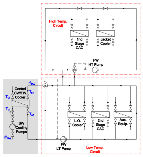
Figure 1.
Typical central cooling system used in marine applications. Explanation of abbreviations: Aux. = Auxiliary, CAC = Charge air cooler, FW = fresh water, L.O. = Lubricant oil, SW = seawater, LT = Low temperature.
The seawater pumps ensure that the required flow rate is provided to the central SW/FW cooler to absorb the heat load, overcoming the pressure losses induced by the system pipelines, fittings, and components as well as the head required for the elevation of seawater. For the conventional case where the SW pump operates at a constant speed, the seawater flow rate is almost constant and the temperature of the seawater exiting the central cooler varies with the cooler heat load and the SW inlet temperature. For the case where variable pump speed is used, the pump speed can be adjusted, so that the seawater flow matches the actual central cooler heat load, taking into account the SW inlet temperature and keeping the seawater exiting temperature as close as possible to the set-point required by the engine manufacturer (in the present study TSW_out ≤ 50 °C).
The LT freshwater cooling system usually consists of two (or three in some cases) pumps [7] to service the main engine (M/E) (scavenging air cooler, lubricating oil cooler and HT freshwater cooler) and the auxiliary machinery components (diesel-electric generator (D/G) sets, air compressor, etc.). The temperature of the freshwater entering the system coolers is controlled by a three-way valve, and in general there are two options: either the three-way valve is continuously adjusted to maintain the temperature level at 36 °C, varying the mass flow rate of FW entering the central cooler, or in case the auxiliary systems are capable of handling cooling water temperatures lower than 36 °C, the three-way valve keeps the heat exchanger by-pass line always closed, except only when the SW temperature is lower than 6 °C to ensure that the FW temperature at the heat exchanger outlet is higher than 10 °C (set-point) as shown in Figure 2 [9].
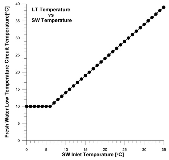
Figure 2.
Variation of fresh water LT system temperature with SW inlet temperature [9]. Explanation of abbreviations: LT = Low Temperature, SW = Sea Water.
The HT freshwater cooling system uses two pumps connected in parallel (one operates while the other remains standby) to provide water for cooling the engine (jacket cooling water circuit). The temperature of the water exiting the engine is adjusted using a three-way valve at a set-point temperature according to the manufacturer’s specifications (usually equal to 80 °C). In many cases, on the HT cooling circuit a Fresh Water Generator (FWG) is incorporated. However, in the present study, the investigation has been focused on the central cooler (left part of Figure 1), assuming that the set-point temperature for the SW outlet from the Central cooler is Tt2 ≤ 50 °C and the FW temperature at the cooler outlet is Ts2 ≤ 36 °C. The control parameter used to ensure that these set-point temperature requirements are satisfied as close as possible to their limit values, is the SW mass flow rate, using a VSD motor for the SW pump. The operation of the SW pumps under variable speed does not affect the HT FW cooling system, where the temperature level is controlled using a separate three-way valve.
The heat exchanger used in the present study for the central cooler is a shell and tube type. The design cooling capacity of the heat exchanger is equal to 4251 kW and its selection is based on a report published by Reference [6] where the central cooling water system of a bulk carrier has been examined with the aim of optimization of the SW cooling pump operation, leading to a corresponding reduction of electric/fuel consumption. Specific characteristics of the heat exchanger considered with the corresponding reference performance data are shown in Table 1.

Table 1.
Design Conditions of the Central Cooler Heat Exchanger [6].
In the present study, the central cooling system comprises two identical heat exchangers and the total cooling load is equally distributed between them, as shown in Figure 3. Three SW pumps are considered each one rated for the 50% of the total pump load (therefore the third one is standing-by). This is one of the most frequently used configurations in practical applications, ensuring adaptable and safe operation of the whole system. In the parametric study conducted one heat exchanger and one SW pump is examined, covering half of the total cooling load. At this point it should be noted that in general, various cooling pump configurations may be considered, i.e., using only one cooling pump or three pumps each rated at 33% of the total pump load required. If only one pump is used, the expected impact from incorporating a VSD is higher compared to the cases where the total pumping load is distributed to more than one pump since in that case there are more options regarding the operational scheme of the pumps as a function of the pumping load and it is easier to effectively adjust the system operation at part-load operating conditions.
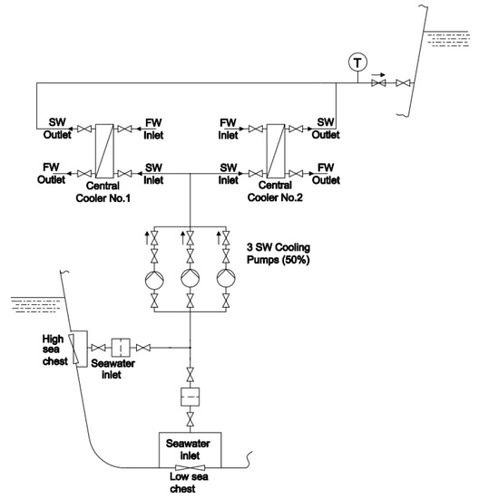
Figure 3.
Typical seawater (SW) cooling system design used in handy-size bulk carriers.
However, the main scope of the current study is to present the advantageous features of the integrated approach proposed to evaluate the operation of the SW pumps installed in variable speed mode, focusing on the optimum control and not on the optimum configuration of the cooling system, and this is why a commonly used pump arrangement has been selected (two SW pumps each one rated for the 50% of the total pump load) to demonstrate the performance of VSD.
3. System Modeling
In the present study, the steady state operation of the central cooling system shown on the left part of Figure 1 is simulated. The main scope is to investigate the potential reduction of the SW pump power demand by adjusting its speed according to the heat load and the SW inlet temperature while satisfying the restrictions set regarding the SW and FW outlet temperatures. To this scope, the central cooler heat exchanger is simulated and the effect of changing the SW mass flow rate and temperatures of SW and FW flow streams is taken into account using first principles.
3.1. Heat Exchanger Model
The heat exchanger examined is a shell and tube type with a total cooling capacity of 4251 kW. The overall heat transfer coefficient U is calculated using the following relation:
where ho is the external convection heat transfer coefficient and hio is the convection heat transfer coefficient of the tube-side fluid referred to the external surface of the tube pipes which is calculated using Equation (3).
where hi is the convection heat transfer coefficient of the tube-side and Di and Do are the internal and external diameter of the tubes. In the present study Di = 0.0147 m and Do = 0.0190 m. The fouling resistance Rf = 0.000176 Km2/W according to Reference [22].
3.1.1. Convection Heat Transfer Coefficient for the Tube-Side Fluid Flow hi
It has been found that the Dittus–Boelter and Colburn equations are not as good as more modern correlations for predicting the Nusselt number in turbulent flow heat transfer through tubes. Mills [23] recommends a correlation due to Gnielinski that dates back to 1976 for smooth tubes [24] and this is used in the present study according to Equation (4). It is noticed that the factor fc is the Fanning friction factor for smooth pipes and is calculated using Equation (5). Gnielinski’s correlation approximates 90% of the published results with 20% accuracy. For Re < 104 the Nusselt number is calculated using Equation (6).
The Prandtl number Pr is calculated using Equation (7), where the fluid properties, i.e., thermal heat capacity cp, viscocity μ and conductivity k, are calculated at the mean SW temperature according to Equation (8). All the fluid properties (seawater or fresh water) are calculated using the expressions proposed by References [20,24,25], taking into account the fluid temperature, pressure and salinity (in case of seawater). Detailed description of the relations used to calculated FW and SW thermophysical properties is given in a separate section below.
where cp is the tube-side fluid isobaric specific heat capacity, μ is the tube-side fluid dynamic viscosity and k is the tube-side fluid thermal conductivity.
The heat transfer coefficient for the tube-side fluid flow hi is calculated by Equation (9) through Nusselt number Nu:
3.1.2. Convection Heat Transfer Coefficient at the Shell-Side Fluid Flow ho
Calculation of the shell-side heat transfer coefficient and pressure drop is considerably more complex than that of the tube side. However, since the main scope of the present study is to capture the relative effect of changing the SW inlet temperature and flow rate on the performance of the central cooler, a simple expression proposed by Reference [26] for a shell with 25% cut segmental baffles, is used. Based on this, the heat transfer coefficient at the shell-side is estimated using Equation (10).
where the Reynolds number is calculated using an equivalent diameter De defined by Equation (11), for a triangular array tube pattern. The tube pitch ratio (defined as Pt/Do) for the specific heat exchanger examined is equal to 1.3368.
It is noticed that in Equation (10), for the calculation of the viscosity correction factor (μ/μw)0.14, the viscosity of the fluid at the wall mean temperature (μw) should be determined. Therefore, an iterative procedure is followed to estimate this term, since it is related to the temperatures of the SW and FW.
3.1.3. Effectiveness of the Heat Exchanger
The SW inlet temperature (Tt1) at the central cooler is an independent variable in the developed model. Based on this temperature (Tt1), the inlet temperature of the FW (Ts1) and the mass flow rates of the SW and FW fluid streams, the effectiveness of the central cooler is calculated through an iterative procedure until the set of the following equation has converged. More specifically the effectiveness of the central cooler is a function of the number of transfer units (NTU) defined as Equation (12) and the heat capacity ratio R′ defined as Equation (13). It is noticed that NTU term is dependent on the overall heat transfer coefficient U, which in turn, is a function of the mass flow rates of SW and FW, as well as the temperatures of both fluid streams. Therefore, the determination of the NTU term is conducted through an iterative procedure [27,28].
The terms and are defined as shown in Equation (14) and in Equation (15).
Having determined the terms NTU and R’, the effectiveness of the central cooler ε is calculated using Equations (16)–(18) according to Reference [28].
where (n) is the number of shell passes and the effectiveness (εα) corresponding to the 1–2 exchanger type configuration is calculated using the following expression:
The effectiveness of the central cooler ε is related to the heat load following Equation (19).
Therefore, having as input the sea-water temperature (Tt1) and the fresh water inlet temperature (Ts1) with the corresponding mass flow rates, the heat transferred (QHX) based on the heat exchanger actual configuration can be determined.
3.2. Calculation of Fresh Water and Seawater Thermophysical Properties
The accurate prediction of seawater thermophysical properties is crucial for the corresponding precise determination of heat transfer dimensionless numbers and heat transfer coefficients used in the thermal performance simulations of seawater heat exchangers. Recently, a FORTRAN program was developed by the present research group for the accurate prediction of fresh water and seawater thermophysical properties. Model development was based on the recent review study of Nayar et al. [20] and the earlier review published by Sharqawy et al. [25]. Nayar et al. [20] reformulated the equations used for the calculation of fresh water and seawater properties, as they were proposed in a previous study by Sharqawy et al. [25] for expanding the dependence of each property not only from temperature and/or salinity but also from pressure. The FORTRAN program developed by our group can predict accurately among others the following seawater thermophysical properties: Vapor pressure, isobaric specific heat capacity, dynamic viscosity and thermal conductivity. Below, the mathematical formulas used for the calculation of the aforementioned fresh water and seawater thermophysical properties are described in detail.
3.2.1. Calculation of Fresh Water and Seawater Vapor Pressure
Seawater vapor pressure calculation according to Nayar et al. [20] is based on the calculation of pure water vapor pressure as described below. Pure water vapor pressure pv,w is calculated in Pa according to the following relation [20]:
where temperature “T” is supplied to the above relation in K. Equation (20) coefficients αi, i = 1…6 are given in the following Table 2:
Table 2.
Coefficients αi, i = 1…6 of Equation (20) used for the calculation of pure water vapor pressure (Reproduced with permission from [20]. Elsevier, 2016).
The following equation is used for the calculation of seawater vapor pressure pv,sw in Pa based on pure water vapor pressure in Pa and seawater salinity “S” in g/kg [20]:
According to Nayar et al. [20], Equation (21) is valid for temperatures “t” [0, 180 °C] and salinities “S” [0, 160 g/kg] and the maximum uncertainty is ±0.26%.
As mentioned above, calculation of pressure-dependent seawater properties such as isobaric specific capacity according to the recent Reference [20] is based on the pressure correction of the pertinent seawater thermophysical properties, which were correlated in 2010 by Sharqawy et al. [25] across the same temperature and salinity range but restricted to reference pressure p0 given by Reference [20]:
where pv,sw(T,S) is the vapor pressure of seawater from Equation (21) in MPa.
3.2.2. Calculation of Seawater Isobaric Heat Capacity
Calculation of seawater isobaric specific heat capacity cp,sw(t,Skg/kg,p,p0) [20] in J/kg-K as function of temperature “t” in °C, salinity “Skg/kg” in kg/kg, pressure “p” and reference pressure p0 in MPa is based on the calculation of seawater isobaric heat capacity cp,sw(t,Skg/kg) at reference pressure p0 as it was proposed in Reference [25].
Seawater isobaric heat capacity cp,sw(t,Skg/kg) at reference pressure p0 is calculated in J/(kg-K) as function of temperature “t” in °C and salinity “Skg/kg” in kg/kg according to the following relation [20]:
where:
The calculation of sea-water isobaric heat capacity cp,sw according to Equation (23) is essential for the final calculation of seawater isobaric heat capacity cp,sw(t,Skg/kg,p,p0) according to the following Equation (28) not only as function of temperature “t” and salinity “Skg/kg” but also as function of seawater pressure “p”. Unlike Reference [20], where seawater isobaric heat capacity cp,sw at reference pressure p0 was expressed as function salinity “S” in g/kg, in this study isobaric heat capacity cp,sw at reference pressure p0 is expressed as function of salinity “Skg/kg” in kg/kg. This modification has been made because feeding of Equations (24)–(27) with salinity in g/kg generated erroneous results regarding isobaric heat capacity. This error in definition of salinity in Reference [20] for use in specific heat capacity can possibly be attributed to typographical error.
Seawater isobaric heat capacity cp,sw(t,Skg/kg,p,p0) is calculated according to the following relation [20] considering also the above-mentioned Equation (23):
where temperature “t” is given in °C, salinity “Skg/kg” in kg/kg, pressure p and reference pressure p0 in MPa. Equation (28) coefficients αi, i = 1…8 are given in Table 3 and Table 4. Variation of seawater isobaric heat capacity with SW temperature, salinity and pressure affects directly the energy balance between SW and FW circuits, as shown in Equations (38) and (39) below, and this has a direct impact on FW temperature and main engine overall cooling load and bsfc.
Table 3.
Coefficients ai, i = 1…4 of Equation (28) used for the calculation of seawater isobaric heat capacity (Reproduced with permission from [20]. Elsevier, 2016).
Table 4.
Coefficients ai, i = 5…8 of Equation (28) used for the calculation of seawater isobaric heat capacity (Reproduced with permission from [20]. Elsevier, 2016).
According to Nayar et al. [20], Equation (28) is valid for temperatures “t” [0, 180 °C], salinities “Skg/kg” [0, 0.18 kg/kg] and pressures “p” [0.1, 1 MPa]. It is also valid for temperatures “t” [0, 180 °C], salinity Skg/kg = 0 kg/kg and pressures “p” [0, 12 MPa]. Equation (28) is also valid for temperatures “t” [0, 40 °C], salinities “Skg/kg” [0, 0.042 kg/kg] and pressures “p” [0, 12 MPa]. In the aforementioned regions of temperature, salinity and pressure the maximum uncertainty of Equation (28), according to Reference [20], is ±1%.
3.2.3. Calculation of Fresh Water and Seawater Dynamic Viscosity
Seawater dynamic viscosity μsw(t,Skg/kg) is calculated in kg/ms as function of temperature “t” in °C and salinity “Skg/kg” in kg/kg according to the following relation proposed by Sharqawy et al. [25]:
where μw(t) is pure water dynamic viscosity in kg/ms, which is calculated according to following relation defined by Sharqawy et al. [25]:
Derivation of Equation (30) in Reference [25] was based on IAPWS 2008 data [27]. The parameters A and B reported in Equation (29) are calculated according to the following relations [25]:
According to Reference [25], Equation (29) is valid for t (0,180 °C) and Skg/kg (0, 0.15 kg/kg) and its accuracy is ±1.5%.
3.2.4. Calculation of Fresh Water and Seawater Thermal Conductivity
Nayar et al. [20] report the following relation, which can be used for the calculation of FW thermal conductivity kW and it is valid within a temperature range of 0–99 °C and a pressure of p0 = 0.1 MPa:
where kw is in W/(m-K) and T* is a dimensionless temperature given by (t + 273.15)/300. Nayar et al. [20] developed a modified version of Equation (33) to consider the effect of pressure variation. Equation (34) gives the ratio of FW thermal conductivity at a given pressure and temperature to that one at 0.1 MPa (calculated by Equation (33)) based on the data given by IAPWS [27].
where:
The new correlation of fresh water thermal conductivity given by Equation (34) is valid within a temperature range of 0–99 °C and a pressure range of 0.1–140 MPa. It has a maximum deviation of 1.1%, and an average deviation of 0.31% from IAPWS [27].
To obtain the thermal conductivity of seawater ksw(t,Skg/kg,p) as a function of temperature, salinity and pressure, the following correlation was used:
The maximum uncertainty of Equation (37) is 2.57% when compared with literature data [20,25].
4. Results and Discussion
In this study, the central cooling system of a handy-size bulk carrier was examined which consisted of two shell and tube heat exchangers and two SW pumps, as shown in Figure 3. The scope of the study was to investigate the overall effect on ship’s total fuel/energy consumption by using a variable speed drive (VSD) SW pump, to adequately adjust the SW mass flow rate according to the corresponding cooling demand and the SW temperature. Therefore, using a VSD cooling pump the change of pumping power demand was calculated relative to the reference case of constant speed pump, based on the pump affinity laws. For each case examined, the FW outlet temperature was maintained as high as possible (approx. 36 °C), while at the same time the corresponding effect on engine bsfc was estimated, due to the relatively increased FW inlet temperature to the charge air cooler. The cooling demand at reference conditions of the central cooling system examined in the present study was distributed to the main engine cooling circuits (Lube oil cooler, Jacket Water Cooler and Scavenge Air Cooler) as well as to the installed auxiliary engines and auxiliary systems, as shown in Table 5 [6].
Table 5.
Distribution of cooling demand at reference conditions [6].
In Table 5 the cooling capacities shown in the column HEAT DISS. (Heat Dissipation) correspond to the maximum expected required cooling capacity of Main and Auxiliary Engines and Systems at tropical conditions (i.e., 45 °C suction air and 36 °C LT-water temperature), while to determine the total cooling design capacity of the central cooler, a load factor (simultaneity factor) was assumed for each component designated in column LOAD on a percentage basis relative to the corresponding maximum load. Based on the above, the total cooling demand (maximum expected) to be covered by the central cooling system was equal to 6465 kW.
The main engine considered in this study was a two-Stroke MAN 5S50ME-C9.7 diesel engine with a Specified Maximum Continuous Rating (SMCR) of 7410 kW at 117 rpm. For the parametric study conducted it was assumed that the cooling load except for the main engine (i.e., regarding auxiliary engines and auxiliary systems) remained constant and equal to the one presented in Table 5 (reference conditions). The variation of the main engine cooling load (distributed in the lube oil, jacket and air charge cooler) as engine load changes was estimated based on engine manufacturer’s specifications and the corresponding Computerized Engine Application System (CEAS) engine data report [21]. In Figure 4 and Figure 5 is presented the variation of the total cooling demand as engine load changes, as well as its distribution to the cooling subsystems of the main engine at the whole range of engine loads examined.
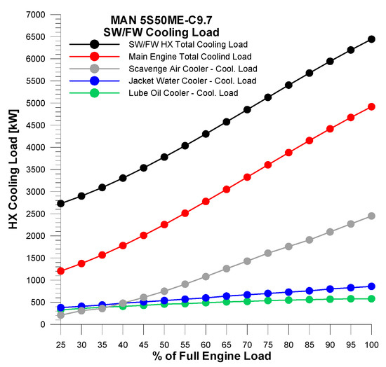
Figure 4.
Variation of the total cooling load demand for the central cooling system of a bulk-size carrier equipped with the MAN 5S50ME-C9.7 two-stroke diesel engine [21].
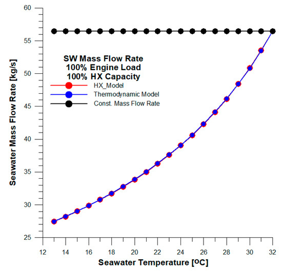
Figure 5.
Comparison of seawater mass flow rates as a function of the SW inlet temperature (Tt1), for central cooler capacity equal to 4251 kW with Variable Speed Drive (VSD) scheme and constant pump speed.
At full engine load the total cooling demand for the central cooling system equaled 6465 kW, which was equally divided to the two heat exchangers considered, i.e., 2 × 3233 kW. The cooling capacity of each HX considered was 4251 kW which is approximately a 30% over-dimensioning according to the usual practice followed in shipyards for safety reasons and to compensate for possible HX efficiency reductions due to fouling [21].
4.1. Estimation of the Required SW Mass Flow Rate
In the present study a parametric investigation was conducted to determine the SW mass flow rate required to cover the cooling load of the central cooling system examined, as the SW HX inlet temperature decreases from its highest value (equal to 32 °C, corresponding to the heat exchanger design/tropical conditions), to a lower temperature equal to 13 °C, with a step of 1 °C, for all the range of main engine loads (25% ÷ 100%). The variation of seawater temperature in the range of 13 ÷ 32 °C is within the typical values found in Mediterranean Sea [29] and covers the majority of the seawater temperatures found in the major sea shipping routes worldwide.
Therefore the SW HX inlet temperature and the main engine load are the independent variables, while the mass flow rate of the FW is maintained constant and equal to the one determined at the heat exchanger design conditions (Table 1), and the control variable is the SW mass flow rate through which the heat capacity of the central cooler is adjusted to ensure that the set-point temperature requirements for the SW outlet (Tt2 ≤ 50 °C) and FW outlet (Ts1 ≤ 36 °C) are satisfied. Since all the parameters of the heat exchanger performance are intrinsically coupled, an iterative procedure is followed and at each step the SW outlet temperature (Tt2), the FW inlet temperature (Ts1) and the FW outlet temperature (Ts2) are determined at steady state conditions, via the energy conservation equation (assuming that there are no heat losses at the central cooler), as shown in Equations (38) and (39).
At first, the effect of SW inlet temperature is examined assuming that the central cooler heat load is equal to the heat exchanger design load QHX = 4251 kW. The parametric study starts with a SW inlet temperature equal to Tt1 = 32 °C (tropical/HX-design conditions), while all the other parameters have values equal to the ones corresponding to the design conditions of the heat exchanger. As SW inlet temperature lowers, a new SW mass flow rate is determined to keep the cooling capacity of the heat exchanger constant (equal to the one corresponding to the heat load examined), while ensuring that the set-point requirements for the SW and FW outlet temperatures are satisfied (i.e., Tt2 ≤ 50 °C and Ts1 ≤ 36 °C).
In Figure 6, the SW mass flow rate () is shown as a function of the SW inlet temperature (Tt1), when the variable speed drive (VSD) scheme is selected, compared to the conventional case where the pump speed remains constant. It is noticed that in the case of the VSD pump being used, two mass flow rates have been determined, i.e., one using a thermodynamic model (namely VSD-Thermodynamic Model) and another using the HX-model (namely VSD-HX Model). The first corresponds to the SW mass flow rate that would be determined using only the energy balance Equation (20), which is the most widely used approach for the techno-economic evaluation of the VSD control on the central cooling pumps, while the second is the SW mass flow rate determined by the proposed methodology in the current study, taking into account how the effectiveness of heat exchanger is affected by the variation of its boundary conditions (temperatures and mass flow rates). It is obvious that as the SW inlet temperature decreases, the required SW mass flow rate decreases too and is almost identical when calculated with either the conventional method (thermodynamic model) or the proposed one (HX-model). This is mainly attributed to the fact that the heat load examined is equal to the design heat load of the heat exchanger, and as will be presented later, this will not be the case at part-load conditions.
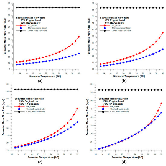
Figure 6.
Comparison of seawater mass flow rates as a function of the SW inlet temperature (Tt1), for central cooler capacities corresponding to (a) 25%, (b) 50%, (c) 75% and (d) 100% of full engine load, with VSD scheme and constant pump speed.
For SW temperature equal to 13 °C, the required SW mass flow rate is approximately 51% lower (27.46 kg/s) than the one corresponding to the constant SW pump speed (56.48 kg/s). The reduction of the SW mass flow rate is followed by a reduction of the SW pump power demand, which can be determined according to affinity laws (Equation (1)) and is equal to 88.5% compared to the constant speed case. This is a considerable reduction, although it should be stated that as the operating point of the pump changes, its efficiency is also affected, and most importantly the VSD and the motor induce additional terms of power losses (variable speed drive efficiency and electric motor efficiency at part loads) which should also be taken into account for precise determination of the actual power reduction of the SW pump [11].
In case the heat load of the central cooler is reduced, i.e., at 25%, 50%, 75% and 100% of full engine load, the variation of the SW mass flow rate as a function of the SW inlet temperature is presented in Figure 7. The heat load of the heat exchanger for each case is estimated based on Figure 5. It can be observed that as the cooling load decreases, there is a higher potential for reducing the SW mass flow rate compared to the HX-design heat load case (4251 kW), leading to approx. an 81% reduction of the SW mass flow rate (10.82 kg/s) at 13 °C compared to the constant pump speed case at 25% of engine load. It is interesting to note that in all part-load cases examined (lower than the HX-design cooling load of 4251 kW), the estimated SW mass flow rate using the proposed method (HX-model) is higher than that obtained using the conventional model (thermodynamic model), with the difference being higher at high SW temperatures. This is attributed to the fact that as the heat load reduces, while the initial FW inlet temperature is high (equal to the HX-design conditions), the estimation of the required SW mass flow rate based only on the heat balance would lead to FW outlet temperatures higher than the ones accepted (Ts2 ≤ 36 °C). An analogous situation may occur with the SW outlet temperature. When the heat load is low and depending on the SW inlet temperature, it is possible that the estimated SW mass flow rate using the conventional heat balance method would be very low, and based on the heat exchanger design configuration, this would lead to SW outlet temperatures higher than the maximum accepted ones (in the present study Tt2 ≤ 50 °C). Therefore, the advantageous feature of the proposed method is that the energy balance equations (used in conventional techno-economic studies for the evaluation of VSD pump drives) are dynamically linked with the actual heat exchanger performance (depending on the boundary conditions, i.e., mass flow rates and temperatures), leading to a more accurate estimation of the required SW mass flow rate as a function of the SW inlet temperature, taking into account all the restrictions of the problem (set-point temperatures).
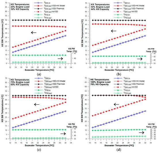
Figure 7.
Comparison of heat exchanger FW and SW inlet and outlet temperatures, with VSD scheme and constant pump speed, for various SW inlet temperatures, at (a) 25%, (b) 50%, (c) 75% and (d) 100% of full engine load.
4.2. Estimation of Heat Exchanger SW and FW Temperatures
Using the method proposed in the present study (HX-model), the tube-side SW and shell-side FW inlet and outlet temperatures from the Heat Exchanger (SW/FW central cooler) are estimated for each SW inlet temperature and at all engine loads examined, i.e., 25%, 50%, 75% and 100% of full engine load. The control parameter is the mass flow rate of SW pump (adjusted using a VSD motor), and the set-point temperatures for the FW outlet is Ts2 ≤ 36 °C and for the SW outlet is Tt2 ≤ 50 °C. As shown in Figure 8, the FW inlet and outlet temperatures are presented on the right vertical axis, while the SW inlet and outlet temperatures on the left vertical axis. Regarding SW outlet temperatures is concerned, there are three different values corresponding to constant SW mass flow rate (conventional case without the usage of VSD pump), the SW mass flow rate estimated using the energy balance Equation (38) with VSD pump (VSD-Thermodynamic) and the SW mass flow rate estimated taking into account the effect on HX effectiveness (HX-model), accordingly.
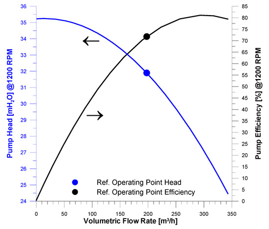
Figure 8.
Head and Efficiency pump characteristic curves at reference pump speed (1200 RPM) and the reference operating point (Flow rate = 197.62 m3/h, Pump Efficiency = 71.8%, Pump Head = 31.90 mH2O).
As observed, the SW outlet temperature using the thermodynamic model is constant and equal to 50 °C at all cases examined (since this is the imposed boundary condition used for the estimation of the required mass flow rate). In contrast, the estimated SW HX outlet temperature using the proposed HX-model is in almost all cases examined lower than the maximum accepted SW outlet temperature (50 °C) with the difference being limited as the engine load increases (approaching the HX-design cooling load). Due to this difference, the estimated required SW mass flow rates using the two methods (i.e., thermodynamic and HX-model) differ as shown in Figure 7. Using the HX-model the reduction of the SW mass flow rate due to the reduced SW inlet temperature at each engine load case examined is limited to fulfill the user-imposed set-point temperature for FW outlet (not to exceed 36 °C). As far as the constant SW mass flow rate case is concerned, it is observed that at each engine load examined, the temperature difference between SW outlet and SW inlet temperature remains constant for all the range of SW inlet temperatures examined, and the SW outlet temperature is always lower than the one estimated using VSD SW pump (as expected).
4.3. Estimation of Fuel Saving Using VSD Cooling Pump
In the standard configuration of the cooling system examined, a constant speed cooling pump is used for the SW cooling circuit, with the characteristic curves presented in Figure 8 and with a pump power demand corresponding to reference operational conditions (Flow rate = 197.62 m3/h, Pump Efficiency = 71.8%, Pump Head = 31.90 mH2O), equal to 24.62 kW. Hence the rated power of the electric motor used to drive the pump is assumed equal to 30 kW. This cooling pump power demand will be used as a reference for the estimation of the relative reduction of the required pumping power when a VSD is used.
According to the power conversion path considered in this study (Figure 9), electric energy is generated by a Diesel Generator unit with a typical brake specific fuel consumption equal to 200 g/kWh, and then this electric power goes through a Variable Frequency Drive (VFD) or variable speed controller which can control electric motor speed by varying the frequency of the electric power supply, and this motor drives the SW pump, covering its power demand. Through this process, three efficiency coefficients are introduced, each one for each component, i.e., for the Variable Speed Drive controller, for the electric motor and for the SW pump accordingly.
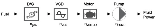
Figure 9.
Schematic presentation of the power conversion path considered for the SW pump.
At part-load conditions and depending on the actual operating point (required SW mass flow rate) the values of these efficiencies vary. Specifically, the motor efficiency at part load is estimated based on the average values suggested by Reference [30] for TEFC (Totally Enclosed Fan Cooled) motors, as shown in Table 6. As far as the effect of part-load operation on VSD efficiency is concerned, this is estimated based on Reference [31], assuming a typical PWM (Pulse Width Modulated) type VFD, as show in Table 7.
Table 6.
Average Efficiencies for Standard Efficiency Motors at Various Load Points for 1200 RPM [30].
Table 7.
Adjustable Speed Drive Part-Load Efficiency (), typical for Pulse-Width-Modulated (PWM) type Variable Frequency Drive (VFD) [31].
As the speed of the SW pump varies (according to the required mass flow rate), its hydraulic efficiency is also affected and is estimated based on the expression proposed by Reference [32] shown in Equation (40), where, is the reference pump efficiency at reference pump speed () and , is the pump speed at each operating condition examined. In the present study, , and RPM.
Based on the above, the wire-to-water efficiency is calculated according to Equation (41):
Assuming a continuous operational profile of the SW cooling pump (just as a reference for the comparative study conducted), i.e., the annual operating hours equal to 8720 h, a total fuel consumption equal to 49.24 tn is estimated for the one SW cooling pump considered.
In the previous section, the required SW mass flow rate has been estimated at each engine load and for all the range of SW inlet temperatures examined, using the proposed HX-model. Based on these mass flow rates, the pump affinity law (Equation (1)), and the wire-to-water efficiency according to Equation (41), the VSD pump power is estimated and the corresponding annual fuel savings are calculated compared to the reference case, and presented in Figure 10, for each engine load and the whole SW inlet temperatures range examined. As expected, the estimated fuel savings are higher at lower engine loads and at lower SW inlet temperatures since in these cases the cooling demand is lower and the required SW mass flow rate is also lower, leading to lower pumping power demand.
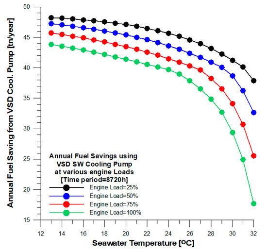
Figure 10.
Estimation of the annual (8720 h) fuel savings obtained substituting constant speed cooling pump with a VSD one (based on SW mass flow rates calculated using the proposed HX-model), for various cooling loads and SW temperatures
It must be stated that the fuel savings estimated in Figure 10, only take into account the operation of the SW cooling pump and disregard the actual effect of reduced SW mass flow rate on the FW outlet temperature and on the engine’s inlet air temperature via the corresponding effect on the performance of the charge air cooler (CAC). However, the scope of this study is to capture the overall effect of substituting the constant speed SW cooling pump with a VSD cooling pump. As shown in Figure 7, when using the VSD cooling pump, the FW outlet temperature is approximately constant and equal to the set-point temperature of 36 °C at all operating conditions examined (irrespective of the SW temperature). In the conventional case of constant speed SW cooling pump, the FW outlet temperature (which is also the scavenge air cooler water inlet temperature) is assumed to be 4 °C higher than the corresponding SW inlet temperature, as suggested by Reference [19] and shown in Figure 2. Moreover, to estimate the effect of ambient conditions on engine’s bsfc, it is assumed that the inlet air temperature () is three degrees higher than the corresponding SW inlet temperature, thus, °C (according to Reference [19] the inlet air temperature is expected to be 1 to 3 °C higher than the corresponding SW temperature).
Based on the aforementioned assumptions and using the MAN publicly available software platform “CEAS Engine Calculations” [21], the effect of seawater temperature on engine’s bsfc is estimated with and without the usage of a VSD SW cooling pump, and presented in Figure 11. It is observed that using a VSD cooling pump, the bsfc is higher at all engine loads examined compared to the conventional case with constant speed SW cooling pump, with the difference being higher as the SW temperature decreases, reaching values up to 1.88 g/kWh.
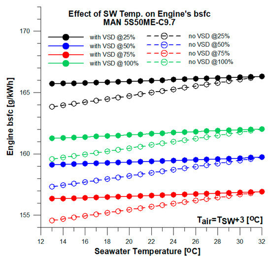
Figure 11.
Comparison of the effect of seawater temperature on engine brake specific fuel consumption (bsfc) [g/kWh] with and without the usage of VSD SW cooling pump at various engine loads.
As shown in Figure 11, the effect of seawater temperature on bsfc is higher in the conventional case (constant speed SW cooling pump) compared to the case with VSD. This is better shown in Figure 12, where the variation of engine’s bsfc is presented as a function of engine load for various SW inlet temperatures with and without VSD SW cooling pump, as estimated using the MAN CEAS software [21]. When using a VSD SW cooling pump, one of the targets set in the iterative procedure followed for the estimation of the required SW mass flow rate is the FW outlet temperature to be as close as possible to the set-point temperature Ts2 = 36 °C. Therefore, the variation of FW outlet temperature when using a VSD SW pump is very limited (as already presented in Figure 7), contrary to what applies in the case of constant speed cooling pump, where the FW outlet temperature is assumed to be 4 °C greater than the corresponding SW temperature. This explains the more intense effect of SW temperature on the engine’s bsfc at constant speed SW pump.
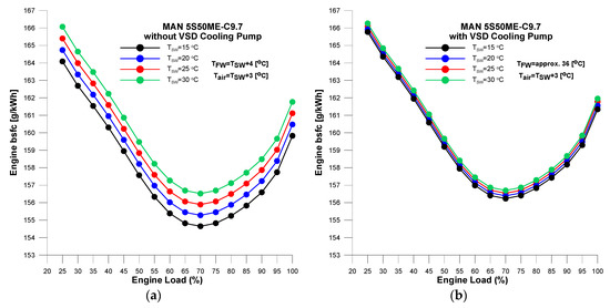
Figure 12.
Comparison of the effect of seawater temperature on engine bsfc [g/kWh] at various engine loads with and without the use of VSD SW cooling pump.
From the analysis above it is obvious that using a VSD SW cooling pump has two contradictory effects on fuel consumption: On the one hand, it has a very strong positive effect on SW cooling pump power demand, which leads to a drastic reduction of the required fuel consumption for the operation of the SW cooling pump, but on the other hand, it leads to increased FW inlet temperature in the charge air cooler which in turn has a small (on a percentage basis) negative effect on the engine’s bsfc. Although as already presented, the relative positive effect on fuel consumption using a VSD pump is significantly higher regarding the power of SW pump compared to the negative effect on engine’s bsfc, one must consider the rated power of these two energy systems. In the case examined in this study, i.e., a handy-size bulk carrier, there are two SW cooling pumps rated at 30 kW each, serving an engine rated at 7410 kW. Combining the effect of VSD cooling pump on engine bsfc and pump power, assuming a continuous annual operation (8720 h) at each engine load and at each seawater temperature examined (only as a basis for our comparative study and not as a realistic operational scenarios), the estimated annual fuel saving (in tn/year) obtained by the substitution of the constant speed cooling pump with a VSD one is presented in Figure 13.
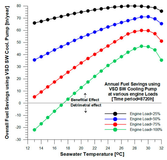
Figure 13.
Comparison of the overall fuel savings (tn/year) obtained using a VSD instead of a conventional constant speed SW cooling pump at various engine loads as a function of the seawater temperature.
As observed, the higher benefit is achieved in lower engine loads, while at full engine load, there is a SW temperature threshold below which the usage of VSD SW cooling pump has a detrimental effect on the total fuel consumption of the main engine and the two cooling pumps. Specifically, at full engine load, when the seawater temperature is lower than 18 °C, it seems that the benefit of using a VSD diminishes, and below that value, using a VSD pump leads to increased fuel consumption compared to the conventional case (constant speed SW cooling pump). Moreover, from the parametric study conducted, it is obvious that at each engine load, the highest prospected benefit from using a VSD cooling pump is observed when the seawater temperature is around 29 °C, while as the seawater temperature decreases this positive effect is reduced.
It should be noted that in the parametric analysis conducted in this study, the required seawater mass flow rate (and consequently the cooling pump power demand) has been estimated having set a target to maintain the FW outlet temperature as close as possible to its reference value of 36 °C, and the SW outlet temperature to be below the maximum accepted value by the class society which is equal to 50 °C. In real life applications, depending on the actual operating conditions (engine load and ambient sea and air temperatures) and using the proposed HX-model to capture the real effect of boundary conditions on the performance of the SW/FW cooler, it is possible to identify the optimum settings for the VSD pump in order to maximize the benefit of lowering the pumping power with the minimum compromise for the bsfc of the engine. One of the main outcomes of the present study is that it has been demonstrated that an integrated approach should be followed to determine the optimum control scheme used for the operation of a VSD cooling pump, to ensure actual fuel savings in real life operating conditions.
5. Conclusions
The main scope of the present work is to propose an adequate methodology for conducting reliable assessments of the potential energy/fuel consumption benefits that can be achieved replacing the conventional constant speed SW cooling pumps with VSD cooling pumps in marine central cooling systems. The two main features of the proposed approach are the following: First, a simple but also physical based HX-model is used to capture the actual effect of changing the boundary conditions on heat exchanger performance, and therefore reliably estimate the required seawater mass flow rate at each operating condition. Second, an integrated approach is followed, also taking into account the detrimental effect on the engine’s bsfc, and the consequent impact of the higher cooling FW inlet temperature to the charge air cooler (CAC) when using a VSD SW cooling pump.
The proposed methodology was applied on a handy-size bulk carrier and a parametric study was conducted to estimate the real effect of substituting the conventional constant speed SW cooling pump with a VSD one, under the whole range of engine loads and for sea-water temperatures ranging from 13 °C up to 32 °C. It was observed that, with the exception of full engine load, in all other cases examined the usage of a VSD SW pump has a positive effect on the total fuel consumption (fuel savings), while at full engine load, there is a threshold temperature of the seawater (equal to 18 °C), under which the operation with a VSD pump (under the control scheme examined in the present study) leads to higher total fuel consumption. At all engine loads examined, the fuel savings estimated using the VSD cooling pump have a maximum value at SW temperatures around 29 °C, while as the SW temperature reduces the total fuel savings decrease.
Overall, it can be concluded that through the proposed integrated approach the SW temperature range was identified for which the optimized operation of a VSD cooling pump can lead to serious annual fuel savings at various main engine loads. It should be noted that the results obtained under the current work correspond to a predefined control scheme for the VSD pump (maintaining the FW outlet temperature as close as possible to 36 °C and the SW outlet temperature lower than 50 °C); however, these parameters can also be adjusted using the proposed integrated approach to maximize the fuel savings attained at each operating condition (engine load, cooling load, ambient conditions) using a VSD cooling pump.
Author Contributions
Conceptualization, E.G.P.; Data curation, E.G.P. and T.C.Z.; Formal analysis, E.G.P.; Investigation, E.G.P.; Methodology, E.G.P.; Project administration, E.G.P.; Software, E.G.P. and T.C.Z.; Writing – original draft, E.G.P. and T.C.Z.; Writing – review & editing, E.G.P., T.C.Z. and J.S.K.
Funding
This research received no external funding.
Conflicts of Interest
The authors declare no conflicts of interest.
Nomenclature
| A | Area (m2) |
| cp | Isobaric specific heat capacity (J/kg-K) |
| De | Equivalent tube diameter (m) |
| Di | Internal tube diameter (m) |
| Do | External tube diameter (m) |
| F | LMTD correction factor |
| hi | Tube-side convection heat transfer coefficient (W/m2-K) |
| hio | External surface tube-side fluid convection heat transfer coefficient (W/m2-K) |
| k | Thermal conductivity (W/m-K) |
| LMTD | Logarithmic mean temperature difference (°C) |
| Mass flow rate (kg/s) | |
| n | Number of shell passes |
| NTU | Number of transfer units |
| p | Pressure (Pa) |
| P | Power (W) |
| Pt | Tube pitch |
| QHX | Heat exchanger cooling capacity (kW) |
| R’ | Heat capacity ratio |
| Rf | Fouling resistance (m2-K/W) |
| S,Skg/kg | Seawater salinity (kg/kg) |
| T | Temperature (K) |
| t | Temperature (°C) |
| Ts1 | Heat exchanger fresh water inlet temperature (°C) |
| Ts2 | Heat exchanger fresh water outlet temperature (°C) |
| Tt1 | Heat exchanger seawater inlet temperature (°C) |
| Tt2 | Heat exchanger seawater outlet temperature (°C) |
| U | Overall heat transfer coefficient (W/m2-K) |
| Volumetric flow rate (m3/s) | |
| Greek | |
| εα | Heat exchanger effectiveness |
| μ | Dynamic viscosity (kg/m-s) |
| Subscripts | |
| atm | Atmospheric |
| fw,FW | Fresh water |
| sw,SW | Seawater |
| v | Vapor |
| w | Pure water |
| Dimensionless numbers | |
| Nu | Nusselt number |
| Pr | Prandtl number |
| Re | Reynolds number |
| Abbreviations | |
| bsfc | Brake specific fuel consumption |
| D/G | Diesel generator |
| FW | Fresh water |
| HT | High temperature |
| HX | Heat exchanger |
| LT | Low Temperature |
| M/E | Main engine |
| SW | Seawater |
| VSD | Variable speed drive |
References
- Corbett, J.J.; Winebrake, J.J.; Green, E.H.; Kasibhatla, P.; Eyring, V.; Lauer, A. Mortality from ship emissions: A global assessment. Environ. Sci. Technol. 2007, 41, 8512–8518. [Google Scholar] [CrossRef] [PubMed]
- IMO. Energy Efficiency Measures. Available online: http://www.imo.org/en/OurWork/Environment/PollutionPrevention/AirPollution/Pages/Technical-and-Operational-Measures.aspx (accessed on 30 June 2019).
- Psaraftis, H.N. Market-based measures for greenhouse gas emissions from ships: A review. WMU J. Marit. Affairs 2012, 11, 211–232. [Google Scholar] [CrossRef]
- Choi, J.; Park, E.-Y. Comparative study on fuel gas supply systems for LNG bunkering using carbon dioxide and glycol water. J. Mar. Sci. Eng. 2019, 7, 184. [Google Scholar] [CrossRef]
- Altosole, M.; Campora, U.; Figari, M.; Laviola, M.; Martelli, M. A diesel engine modelling approach for ship propulsion real-time simulators. J. Mar. Sci. Eng. 2019, 7, 138. [Google Scholar] [CrossRef]
- Bro, G.-C. Optimisation of pump- and cooling water systems, Report Member of Green Ship of the Future, APV and DESMI. 2008. Available online: https://www.scribd.com/document/273383831/APV-DESMI-CARL-BRO-optimisation-of-pump-and-cooling-water-systems-pdf (accessed on 30 June 2019).
- DNV GL SE. Rules for classification and construction, I-1.2. Hamburg, Germany. Available online: http://www.gl-group.com/infoServices/rules/pdfs/gl_i-1-2_e.pdf (accessed on 20 June 2016).
- Rasanen, J.-E.; Schreiber, E.W. Using Variable Frequency Drives (VSD) to save energy and reduce emissions in newbuilds and existing ships, Energy efficient solutions, White Paper, ABB Marine and Cranes. Available online: https://library.e.abb.com/public/a2bd960ccd43d82ac1257b0200442327/VFD%20EnergyEfficiency_Rasanen_Schreiber_ABB_27%2004%202012.pdf (accessed on 30 June 2019).
- Skeltved, O. Central Cooling System: LT cooling system with low/high temperature. Available online: https://www.academia.edu/31531713/CENTRAL_COOLING_SYSTEM_LT_cooling_system_with_low_high_temperature (accessed on 30 June 2019).
- Giannoutsos, S.V.; Manias, S.N. A data-driven process controller for energy-efficient variable-speed pump operation in the central cooling water system of marine vessels. IEEE Trans. Ind. Electr. 2015, 62, 587–598. [Google Scholar] [CrossRef]
- Theotokatos, G.; Sfakianakis, K.; Vassalos, D. Investigation of ship cooling system operation for improving energy efficiency. J. Mar. Sci. Technol. 2017, 22, 38–50. [Google Scholar] [CrossRef]
- Su, C.-L.; Chung, W.-L.; Yu, K.-T. An energy-savings evaluation method for variable-frequency-drive applications on ship central cooling systems. IEEE Trans. Ind. Appl. 2014, 50, 1286–1294. [Google Scholar]
- Zymaris, A.S.; Alnes, O.-A.; Knutsen, K.-E.; Kakalis, N. Towards a model-based condition assessment of complex marine machinery systems using systems engineering. In Proceedings of the Third European Conference of the Prognostics and Health Management (PHM) Society, Bilbao, Spain, 5–8 July 2016. [Google Scholar]
- Mrakovcic, T.; Medica, V.; Skific, N. Numerical modelling of an engine cooling system. J. Mech. Eng. 2004, 50, 104–114. [Google Scholar]
- Hansen, M.; Stoustrup, J.; Bendtsen, J. Modeling and control of a single-phase marine cooling system. Control Eng. Pract. 2013, 21, 1726–1734. [Google Scholar] [CrossRef]
- Kocak, G.; Durmusoglu, Y. Energy efficiency analysis of a ship’s central cooling system using variable speed pump. J. Mar. Eng. Tech. 2017, 43–51. [Google Scholar] [CrossRef]
- Boulougouris, E.K.; Papanikolaou, A.D.; Pavlou, A. Energy efficiency parametric design tool in the framework of holistic ship design optimization. Proc. IMechE Part M J. Eng. Marit. Environ. 2011, 225, 242–260. [Google Scholar] [CrossRef]
- Coraddu, A.; Figari, M.; Savio, S. Numerical investigation on ship energy efficiency by Monte Carlo simulation. Proc. IMechE Part M J. Eng. Marit. Environ. 2014, 228, 220–234. [Google Scholar] [CrossRef]
- MAN Diesel & Turbo. Influence of Ambient Temperature Conditions Main engine operation of MAN B&W two-stroke engines. 2010. Available online: https://www.tradewindsnews.com/incoming/314436/man-twostroke-engine-reportpdf/binary/MAN%20two-stroke%20engine%20report.pdf (accessed on 30 June 2019).
- Nayar, K.G.; Sharqawy, M.H.; Banchik, L.D.; Lienhard, J.H.V. Thermophysical properties of seawater: A review and new correlations that include pressure dependence. Desalination 2016, 390, 1–24. [Google Scholar] [CrossRef]
- CEAS Engine Calculations. MAN B&W - MAN Energy Solutions. Available online: https://marine.man-es.com/two-stroke/ceas (accessed on 30 June 2019).
- Harrison, J. Standard of Tubular Exchanger Manufacturers Association, 8th ed.; TEMA: New York, NY, USA, 1999. [Google Scholar]
- Mills, A.F. Heat Transfer, 2nd ed.; Richard D. Irwin, Inc.: Boston, MA, USA, 1992. [Google Scholar]
- Gnielinski, V. New equations for heat and mass transfer in turbulent pipe and channel flow. Int. Chem. Eng. 1976, 16, 359–368. [Google Scholar]
- Sharqawy, M.H.; Lienhard, J.H.V.; Zubair, S.M. Thermophysical properties of seawater: A review of existing correlations and data. Desalin. Water Treat. 2010, 16, 354–380. [Google Scholar] [CrossRef]
- Cao, E. Heat Transfer in Process Engineering; McGraw-Hill: New York, NY, USA, 2010. [Google Scholar]
- International Association for the Properties of Water and Steam (IAPWS). Available online: http://www.iapws.org (accessed on 30 June 2019).
- Kern, D. Process Heat Transfer; McGraw-Hill: New York, NY, USA, 1954. [Google Scholar]
- Sea Temperature. Available online: https://www.seatemperature.org (accessed on 30 June 2019).
- US Department of Energy. Fact Sheet: Determining Electric Motor Load and Efficiency; Technical Report for Motor Challenge Program; US Department of Energy: Washington, DC, USA, 1991.
- US Department of Energy. Adjustable Speed Drive Part-Load Efficiency; Technical Report for Energy Efficiency and Renewable Energy; US Department of Energy: Washington, DC, USA, 2012.
- Sârbu, I.; Borza, I. Energetic optimization of water pumping in distribution systems. Period. Polytech. Ser. Mech. Eng. 1998, 42, 141–152. [Google Scholar]
© 2019 by the authors. Licensee MDPI, Basel, Switzerland. This article is an open access article distributed under the terms and conditions of the Creative Commons Attribution (CC BY) license (http://creativecommons.org/licenses/by/4.0/).