U-Net-Based Daytime and Nighttime Prediction of Surface Suspended Sediment Concentrations in Wenzhou Coastal Waters

Abstract

This study constructs a time-dependent model to predict the nighttime suspended sediment concentration near Wenzhou based on the convolutional neural network U-Net, which integrates the high-resolution Delft3D (version 4.03.01) hydrodynamic model and GOCI satellite observation data. The model’s prediction accuracy is significantly improved by replacing the original tide level with the tide level variation and increasing the temporal resolution of the flow field to 15 min via sensitivity analysis of the model’s input parameters. The validation results show that the model can maintain high consistency with GOCI observations in short-term prediction, with a structural similarity index (SSIM) of 0.82. For multi-hour continuous nighttime predictions, while quantitative uncertainty increases with the forecast horizon, the model successfully captures the spatial evolution patterns and maintains stable structural characteristics. The model effectively provides missing remote sensing nighttime observations as well as a new method for full-cycle prediction of nearshore SSC.

1. Introduction

The suspended sediment concentration (SSC) is a key water quality parameter of marine ecosystems that directly affects attributes of water bodies such as their transparency, turbidity, and color [1,2]. Suspended sediment has a large specific surface area [3,4], which enables it to adsorb nutrients and pollutants; when runoff is transported away from the water body, it influences the distribution of nutrients and pollutants, which can impact nearshore biogeochemical processes [5,6]. In addition, changes in suspended sediments have important implications when dredging harbor channels and constructing nearshore projects [7,8].

Traditional tools for monitoring suspended sediment include field measurements, satellite remote sensing inversion, and numerical simulation analysis, but these methods have their own limitations [9]. For example, the accuracy of field measurements is relatively high, but they are time-consuming, have high labor costs, and are susceptible to the influence of natural factors such as weather. Additionally, sampling is conducted in a spatially dispersed manner and cannot cover a large area; thus, sampled data are often insufficient for use on the spatial and temporal scales of large-area continuity [10]. In contrast, numerical simulation methods can effectively simulate macro-scale suspended sediment concentration variations [11]; however, given that sediment deposition rates are influenced by a variety of factors, including water viscosity, particle size and shape, and density differences between water and particles, numerical simulations are unable to finely calibrate sedimentological parameters at each node within the sample grid [12,13]. Therefore, it is difficult to improve the computational efficiency of sediment modeling to ensure its accuracy when simulating large-scale sediment distribution compared to simple hydrodynamic models [14]. Conversely, satellite remote sensing has the advantages of a high spatial resolution, short revisit period, and large coverage area [15]. However, due to the influence of weather conditions such as cloud cover on the operation time and temporal resolution, satellite remote sensing can only obtain the distribution of suspended sediment at some moments of the day at most; it is unable to monitor suspended sediment dynamics at night when there is no sunlight, which significantly reduces its practical value.

Convolutional Neural Networks (CNNs) are increasingly used as a tool for water quality prediction because they handle non-linear data features well [16]. Previous works, such as the Chlorophyll-a retrieval model by Sun et al. [17] and the turbidity estimation model using U-Net by Zhang et al. [18], demonstrate the potential of deep learning in mapping the relationship between optical parameters and environmental factors. Despite these advances, current research has mostly focused on direct inversion based on daytime images. There is still a lack of studies that use deep learning to integrate the continuous output of numerical models with high-precision satellite data to specifically address the data gap during nighttime.

To bridge this nighttime data gap, this study develops a deep learning framework that assimilates high-resolution Delft3D hydrodynamic simulations with Geostationary Ocean Color Imager (GOCI) observations. A CNN was employed to establish a mapping relationship between hydrodynamic variables and satellite-derived SSC. A total of 400 matched data pairs (comprising hydrodynamic parameters and corresponding GOCI images) from July to August (2015–2019) were collected to train and validate the machine learning models. This approach successfully realizes continuous 24-h SSC prediction, effectively reconstructing missing nighttime information while maintaining a high accuracy and computational efficiency compared to those of traditional complex sediment transport models.

2. Data and Methods

2.1. Study Area

This study focuses on the coastal waters off Wenzhou, southeastern Zhejiang Province, a region characterized by extensive silty tidal flats (Figure 1). Unlike typical river-dominated estuaries, the sediment budget in this area is governed primarily by marine dynamics rather than terrestrial runoff. Quantitative analyses of seabed siltation [19] demonstrate that land-derived input is negligible; rather, the sediment accumulation is attributed to the shoreward transport of offshore materials driven by the interaction of tidal currents and waves. This unique transport mechanism renders the nearshore morphodynamics highly sensitive to external perturbations. Notably, recent large-scale anthropogenic interventions, particularly the Oufei Beach reclamation project, have significantly altered the local hydrodynamic regime [20]. Consequently, accurate prediction of surface SSC is imperative for evaluating the ecological stability and environmental response to such intensive coastal engineering.

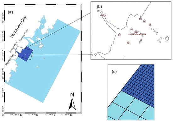
Figure 1. The study area and model mesh setup. (a) The computational domain covering the Wenzhou coast; the dark blue area denotes the local grid refinement at the Oufei Shoal. (b) Spatial distribution of the observation stations, where Ruian and Shangganshan represent tide level stations, and D1–D8 represent current velocity and direction observation stations. (c) Detailed view of the grid resolution, with grid sizes of 500 m × 500 m for the coarse domain (light blue) and 100 m × 100 m for the refined area (dark blue).

To evaluate the applicability of this U-Net-based approach elsewhere, it is important to note the characteristic features of this location. The Wenzhou coastal area represents a typical high-turbidity environment dominated by strong semi-diurnal tides. These conditions ensure that the Delft3D model provides strong physical constraints on sediment transport, while the GOCI sensor captures high-contrast optical signals, both of which are critical for the successful fusion of numerical models and deep learning.

2.2. Data Sources and Preprocessing

2.2.1. GOCI Satellite Data and Preprocessing

This study used GOCI (Geostationary Ocean Color Imager) (KIOST, Busan, Republic of Korea) remote sensing data from July 1 to August 15 of each year from 2015 to 2019. The months of July and August were chosen because there are more hours of clear skies in the sea area in summer, and so the satellite data are highly efficient. GOCI, as the world’s first geostationary ocean remote sensing satellite, has eight bands covering from visible to near-infrared, with a temporal resolution of one hour, and it can acquire eight images per day from 0:00 to 7:00 (UTC) [21]. While this study period theoretically provides approximately 1800 potential hourly observation windows, we implemented a stringent Quality Control (QC) procedure, resulting in the final selection of 400 high-quality matched samples to ensure the reliability of the dataset. As introduced in the following Section 2.3, we manually identified and removed satellite observations contaminated by cloud artifacts or occlusion to ensure data robustness.

To address the challenge of the Wenzhou coastal waters’ high turbidity, the SSC inversion algorithm developed by He et al. [22] was adopted. This algorithm, specifically designed for turbid coastal environments, utilizes the 490 nm and 745 nm bands to significantly improve retrieval accuracy and stability:

$$SSC={10}^{1.0758+1.1230\times {\displaystyle \frac{R_{\mathrm{rs}}\left(745\right)}{R_{\mathrm{rs}}\left(490\right)}}}$$

(1)

In the equation, SSC represents the suspended sediment concentration (mg/L), while Rrs denotes the remote sensing reflectance.

To address cloud contamination, an empirical masking algorithm based on the spectral relationships between adjacent bands was adopted [23].

Due to severe cloud occlusion, localized data are often missing in remote sensing images. In this study, the Data Interpolating Empirical Orthogonal Functions (DINEOF) method [24] is applied to reconstruct the missing data, and the comparison between the original and reconstructed fields is shown in Figure 2. This method is based on the spatial and temporal correlation of the data itself for adaptive modeling, without relying on external a priori information, and can effectively extract the main modal features in the time series.

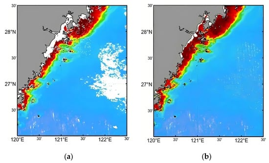
Figure 2. Comparison of GOCI-derived SSC fields before and after data reconstruction. (a) Original SSC data with missing pixels due to cloud cover. (b) Reconstructed SSC field using the DINEOF method. The color scale indicates the concentration of SSC, ranging from blue (low) to red (high).

2.2.2. Wind Field Data

The wind field data used in this study come from the reanalysis products of ERA5 (European Reanalysis Center for Medium-Range Weather Forecasts), which include meridional and latitudinal wind speeds at a height of 10 m, across the time period of 1 July and 15 August 2015–2019, with a temporal resolution of 1 h and a spatial resolution of 0.25°. In order to maintain consistency with the Delft3D model grid of the study area, spatial reprojection and grid interpolation were performed in this study for the ERA5 wind field using a bilinear interpolation method, which resulted in a 0.005° grid coverage consistent with the model.

Prior to model training, a rigorous quality control (QC) procedure was applied. Satellite observations contaminated by cloud artifacts or impacted by typhoons were identified as outliers and manually removed. Consequently, the corresponding wind field data during these extreme events were excluded to ensure the robustness of the training set and avoid introducing noise from extreme irregularities. The processed wind data were deemed sufficient to effectively drive the hydrodynamic simulations.

2.2.3. Hydrodynamic Modeling Setup

In terms of hydrodynamics, this study constructed a numerical model of the tidal currents off the Wenzhou shore based on the Delft3D open source software, and the flow field and tide level data in the study area were obtained through simulation. The model calculation area is off the Wenzhou shore, with a longitude range of 120.3 °E–122 °E and a latitude range of 26.8 °N–28.4 °N. In order to improve the simulation accuracy of the key areas, the model adopts a locally encrypted grid with a resolution of 100 m × 100 m; the rest of the area adopts a resolution of 500 m × 500 m.

River discharge boundaries were applied at the upstream limits, while the open sea boundary employed tidal harmonic constants from the global tidal model TPXO as the tidal driving factor. Specifically, fifteen primary and shallow-water tidal constituents—M2, S2, K1, O1, N2, P1, Q1, K2, S1, M4, MN4, MS4, MM, MF, and 2N2—were selected as tidal level drivers for the open ocean boundary.

The topographic data were obtained from the 2019 bathymetric survey data, using a combination of the GPS-RTK (Trimble, Sunnyvale, CA, USA) (without tide gauge mode) and DGPS (Trimble, Sunnyvale, CA, USA) (with tide gauge mode) positioning methods, together with a single-beam sounder to obtain the bathymetric data, and measurements were taken using the cross-section method. Then, the bathymetric data were uniformly converted to the CGCS2000 coordinate system, and the Kriging interpolation method was used to construct a digital topographic seafloor model of the study area, which was then matched with the Delft3D model grid as the model bottom bed input.

The computation time of the model is July–August 2015–2019, and the model is run in the hot-start mode, with a time step of 1 min and an output interval of 15 min, using the measured data as the rate determination and validation. Figure 3 and Figure 4 show the flow field validation results at representative stations. As can be seen from the figures, the numerical simulation results and the measured data have good consistency in the overall trend and amplitude, indicating that the numerical model of tidal currents constructed in this paper can accurately reproduce the tides and tidal currents in the study area.

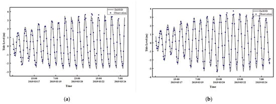
Figure 3. Comparison of observed and simulated tidal level variation at Ruian and Shangganshan stations. (a) Ruian station; (b) Shangganshan station.

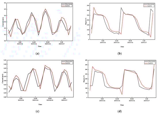
Figure 4. Comparison of observed and simulated current speed and direction at stations D4 and D8: (a) current speed at Station D4; (b) current direction at Station D4; (c) current speed at Station D8; (d) current direction at Station D8.

2.3. Model Architecture and Training Methods

In this study, we adopt the fully symmetric encoding–decoding structure of the convolutional neural network model U-Net. Compared with traditional convolutional neural networks, the U-Net structure improves the feature extraction and expression ability of the model by introducing a large number of feature channels, which enables the shallow features to be passed to the deeper network more efficiently on a smaller-scale training dataset.

The encoder component of the U-Net model accepts an input tensor with dimensions of 12 × 321 × 341 (Channels × Height × Width) and consists of three cascaded modules. Each module consists of two layers of 3 × 3 convolutional operations with ReLU activation functions, followed by spatial downsampling through maximal pooling. The number of channels in the feature map is increased step by step after each downsampling to 64, 128, 256, and 512 in order to gradually extract deeper image features. In the decoding stage, each decoding module first performs an upsampling operation (UpSampling2D, implemented via PyTorch version 2.6.0) to recover the spatial resolution of the feature map. Subsequently, the features are fused with the feature maps of the corresponding layers in the encoder through a skip connection. The fused feature maps are subjected to two convolutional processes with ReLU activation, which are used to gradually recover the spatial information and compress the channel dimensions. The final output layer employs a 1 × 1 convolutional layer in order to generate predictions for the target variables, with an output size of 1 × 321 × 341, corresponding to a single-channel SSC distribution map.

Regarding data preprocessing, errors arising from remote sensing observations and inversion algorithms were rigorously addressed. First, the Interquartile Range (IQR) method was applied to identify and remove statistical outliers. Furthermore, time periods with significant data gaps caused by typhoons or heavy cloud cover were manually excluded. To address the spatial inconsistency among remote sensing data, reanalysis products, and numerical model outputs, all datasets were unified to a 0.005° spatial resolution. Importantly, data were extracted for every intersection of the standardized grid (321 × 341 grid points) covering the entire study area, ensuring that each sample represents a complete spatial field rather than discrete site observations. This resulted in 400 valid matched samples. The target variable is the suspended sediment concentration (SSC), while the input auxiliary variables include wind speed components (zonal u and meridional v), current velocity components (zonal u and meridional v), and tidal level. Specific variable configurations are detailed in Table 1.

Table 1. Comparison between raw data and model input data. Note: UTC: Coordinated Universal Time; "/" indicates no data or not available.

Data Type	Raw Data				Model Input Data
	Temporal Resolution	Spatial Resolution	Data Source	Number of Scenes	Temporal Resolution	Spatial Resolution	Data Source	Number of Scenes
Observed SSC	1 h (00:00–07:00 UTC)	500 m	GOCI	1	1 h (00:00–07:00 UTC)	0.005°	GOCI	1
Predicted SSC	1 h (08:00–23:00 UTC)	/	/	/	1 h (08:00–23:00 UTC)	0.005°	U-Net	1
Wind Field	1 h	0.25°	ERA5	1	1 h	0.005°	ERA5	1
Flow Field	1 h	<500 m	Delft3D	1	15 min	0.005°	Delft3D	4
Tidal Level	1 h	<500 m	Delft3D	1	/	/	/	/
Tidal Level Difference	/	/	/	/	1 h	0.005°	Delft3D	1

In the forecasting phase, two distinct scenarios were designed. For short-term (one-h) forecasting, the model takes the current hydrodynamic conditions and SSC as input to directly output the predicted SSC for the next time step. For extended forecasts, such as 16-h nighttime projection, there is an inherent absence of satellite-derived SSC observations during the night. Thus, the model first generates a 1-h forecast; this predicted result is then combined with the corresponding hydrodynamic variables of the next time point to serve as the input for the subsequent step. Through this iterative process, the model simulates the temporal evolution of SSC over the next 16 h.

To achieve the prediction objectives, this study constructs a U-Net model based on the PyTorch (version 2.6.0) framework. Crucially, to eliminate potential temporal bias and ensure a representative data distribution, the entire dataset was randomly shuffled prior to splitting. Consequently, the first 300 samples of the randomized dataset were designated for training, while the remaining samples were reserved for validation. The model was optimized using the Adam optimizer with an initial learning rate of 10–3 and a batch size of 12. During the training phase, the input data were further shuffled within each epoch to prevent the model from converging to local optima. The training process was conducted for 1000 epochs.

To evaluate the performance of the U-Net model, the Mean Squared Error (MSE) was adopted as the loss function, which is defined as:

$$MSE={\displaystyle \frac{1}{n}}{\sum }_{i=1}^n(y_i-{\widehat{y}}_i{)}^2,$$

(2)

In the equation, $n$ represents the total number of samples, $y_i$ denotes the true SSC value, and ${\widehat{y}}_i$ represents the predicted SSC value.

As can be seen from Figure 5, the model converges rapidly in the first 20 training epochs, indicating that the model can learn the main relationship between SSC and hydrodynamic environmental parameters relatively quickly. The MSE of the subsequent training and validation sets decreases slowly, indicating that the model further optimizes its ability to fit detailed features on top of the initial convergence.

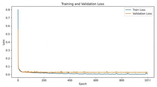
Figure 5. Training and validation loss curves of the U-Net model.

2.4. Model Evaluation Metrics

In order to comprehensively evaluate the prediction performance of the model, three metrics are employed as evaluation criteria: the structural similarity index (SSIM), Root Mean Squared Error (RMSE), and Mean Absolute Percentage Error (MAPE). The formulas for calculating SSIM, RMSE, and MAPE are as follows:

$$SSIM\left(x,y\right)={\displaystyle \frac{\left(2{\mu }_x{\mu }_y+C_1\right)\left(2{\sigma }_{xy}+C_2\right)}{\left({\mu }_x^2+{\mu }_y^2+C_1\right)\left({\sigma }_x^2+{\sigma }_y^2+C_2\right)}},$$

(3)

In the formula, ${\mu }_x$ and ${\mu }_y$ represent the mean values of the two images, ${\sigma }_x$ and ${\sigma }_y$ denote their standard deviations, ${\sigma }_{xy}$ is the covariance between the two images, and $C_1$ and $C_2$ are constants used to maintain stability (preventing the denominator from becoming zero).

$$RMSE=\sqrt{{\displaystyle \frac{1}{n}}{\sum }_{i=1}^n(y_i-{\widehat{y}}_i{)}^2},$$

(4)

$$MAPE={\displaystyle \frac{{\displaystyle \sum _{i=1}^n\frac{|y_i-{\widehat{y}}_i|}{y_i}\times 100\%}}{n}},$$

(5)

where the parameters $n$, $y_i$ and ${\widehat{y}}_i$ are defined as previously described in Equation (2).

3. Result Analysis and Discussion

3.1. Sensitivity Analysis of Model Input Parameters

To investigate the model’s sensitivity to different hydrodynamic forcings, three input configurations were evaluated, as detailed in Table 2. Scheme 1 utilizes wind and current fields only; Scheme 2 introduces the absolute tidal level; and Scheme 3 integrates the temporal tidal variation (calculated as the difference in the tidal level between adjacent time steps).

Table 2. Comparison of model prediction accuracy under different parameter input schemes (Schemes S1–S3). S1: wind and flow fields; S2: wind, flow fields, and absolute tidal level; S3: wind, flow fields, and temporal tidal level difference.

Scheme	Input Combination	RMSE (mg/L)	MAPE (%)	SSIM
S1	Wind field + Flow field	39.56	22.31	0.61
S2	Wind field + Flow field + Tidal level	22.43	11.48	0.77
S3	Wind field + Flow field + Tidal level difference	20.33	10.82	0.82

The results show that Scheme 3, i.e., flow field, wind field, and tide level variation, is better than Scheme 1 and Scheme 2 in terms of three indexes: Scheme 3 obtained the lowest RMSE value, the smallest MAPE value, and the highest SSIM value (20.33 mg/L, 10.82% and 0.82, respectively). These findings underscore the critical role of tidal variation features. Unlike absolute tidal levels, the rate of tidal change serves as a better proxy for dynamic processes—tidal pumping and sediment resuspension—thereby significantly improving the model’s ability to capture complex sediment transport and redistribution mechanisms.

Figure 6 provides a spatial visualization of the forecasting performance across the three experimental configurations. Evidently, Scheme 3 (incorporating tidal variation) is superior in resolving the spatial heterogeneity and gradient characteristics of the SSC field. Notably, Figure 6d,h demonstrate that Scheme 3 captures detailed structural features within complex estuarine and frontal zones. Conversely, Scheme 1 and Scheme 2 show distinct discrepancies in gradient transitions and fail to accurately reproduce low-concentration regions. Physically, the rate of tidal change serves as a critical proxy for hydrodynamic dynamism. It implicitly encodes variations in current acceleration and direction, which are the primary drivers of sediment resuspension and settling. In macro-tidal environments, substantial tidal variations enhance hydrodynamic disturbance and sediment redistribution [25], thereby significantly shaping the spatiotemporal patterns of SSC.

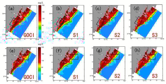
Figure 6. Visual validation of the prediction results for Scenarios 1–3 (S1–S3) using GOCI satellite imagery. The comparison is conducted at two representative timestamps: (a–d) correspond to the first moment, and (e–h) correspond to the second moment. The black rectangles highlight regions with significant SSC gradients for detailed visual inspection. The black rectangles (boxes) represent typical regions of SSC variation for detailed visual inspection. Note: While the global RMSE indicates limitations in quantitative precision for long-term forecasts, the visualized contours highlight the model’s capability to capture spatial morphological structures (e.g., the evolution of sediment fronts and plume boundaries), effectively reflecting the relative spatial distribution of the SSC field.

To make the input features, such as flow velocity and flow direction, reflect the hydrodynamic processes on short time scales more accurately, the temporal resolution of the flow field in this study is refined from 1 h to 15 min to obtain more detailed information on tides, transient flow velocity, and local perturbations, and to enhance the model’s sensitivity to local hydrodynamic perturbations and the prediction accuracy of the changes in the SSC. That is, in the model input stage, each scene of SSC corresponds to four scenes of flow field data to characterize the temporal details of the hydrodynamic features, which further enhances the model’s ability to portray the tidal process and transient dynamic effects.

3.2. Model Prediction Results and Validation

In order to comprehensively assess the forecast performance of the constructed SSC prediction model at different forecasting timescales, different forecasting steps are selected to validate the model used in this study to reflect its accuracy in short-time forecasting and its stability in long-time forecasting.

Figure 7 demonstrates the reconstruction results of the spatial distribution of SSC at different prediction time scales. As shown in Figure 7b,d,f,h, even under different timescales, the model is still able to effectively capture the detailed evolution of the sediment concentration gradient and the spatial differences in the SSC gradients in the inlet region, which demonstrates its ability to portray the distribution of the sediment concentration under complex hydrodynamic backgrounds with strong stability. This is attributed to the fact that the adopted U-Net structure introduces multi-scale feature channels in the design, so that shallow information can be efficiently transferred to the deep network to enhance the feature extraction and expression ability, thus accurately capturing the main pattern of SSC distribution and key regional features as well as reflecting the adaptability of the model to the spatial and temporal variations in SSC.

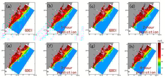
Figure 7. Comparison of model prediction performance at different forecast durations: (a,c,e,g) display the ground truth SSC retrieved from GOCI satellite data. (b,d,f,h) present the corresponding model predictions for 1-h, 2-h, 3-h, and 4-h lead times, respectively. Note: While the global RMSE indicates limitations in quantitative precision for long-term forecasts, the visualized contours highlight the model’s capability to capture spatial morphological structures (e.g., the evolution of sediment fronts and plume boundaries), effectively reflecting the relative spatial distribution of the SSC field.

Table 3 shows that when comparing different forecast periods, the model displays significant efficiency in short-term forecasting, with RMSE, MAPE, and SSIM values of 20.33 mg/L, 10.82% and 0.82, respectively. As the forecast period extended to 16 h, the RMSE and MAPE values increased to 45.57 mg/L and 32.27%, respectively, and the SSIM decreased to 0.57.

Table 3. Comparison of model prediction accuracy at different prediction lead times.

Prediction Horizon (h)	RMSE (mg/L)	MAPE (%)	SSIM
1	20.33	10.82	0.82
2	28.57	11.15	0.79
3	34.35	11.57	0.73
4	37.61	14.24	0.69
8	41.05	21.14	0.63
16	45.57	32.27	0.57
Average	34.58	16.86	0.71

It is important to note the statistical limitations of these longer-term forecasts. Following the evaluation criteria by Prairie (1996) [26], while the quantitative precision decreases with the forecast horizon, effectively resolving data into broad categories (e.g., high vs. low turbidity), the model retains significant value due to the high spatial heterogeneity of coastal SSC.

However, it should be emphasized that this global RMSE is a spatially averaged metric. The SSC distribution in Wenzhou coastal waters is highly skewed, with large errors disproportionately driven by the high-concentration nearshore zones (Turbidity Maximum Zone). In offshore areas where the background SSC is lower, the absolute prediction error is significantly smaller. Consequently, despite the limitations in global metrics, the model retains finer resolving power in these sub-regions. Furthermore, as shown in Figure 6, Figure 7 and Figure 8, the model successfully captures spatial morphological structures, such as the movement of sediment fronts, providing valuable qualitative information beyond simple point-wise regression.

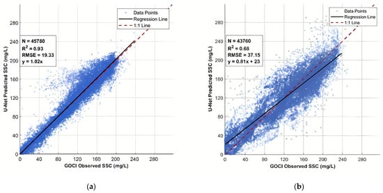
Figure 8. Comparison of GOCI-observed and U-Net predicted SSC for recursive multi-step forecast horizons: (a) 1-h lead time (T + 1); (b) 16-h lead time (T + 16). The dashed red line represents the 1:1 reference line, and the solid black line denotes the linear regression.

To comprehensively evaluate the model’s predictive performance, a pixel-wise validation was conducted across the entire study area. Instead of selecting specific sites, we compared the predicted values against GOCI-observed data at each valid marine grid intersection (321 × 341 grid). The N value here represents the total count of valid marine pixels after land masking and data filtering, ensuring that the statistical metrics reflect the model’s spatial consistency across the complex hydrodynamic environment of the Wenzhou coastal area.

As illustrated in Figure 8, the pixel-wise validation for representative recursive prediction horizons shows that at the 1-h lead time (T + 1, N = 45,780), the model achieves an R² of 0.93 and an RMSE of 19.33 mg/L (y = 1.02x), which suggests a general maintenance of spatial structures with relatively low systematic bias. As the horizon extends to 16-h (T + 16, N = 43,760), the R² and RMSE reach 0.68 and 37.15 mg/L, respectively; although the scatter distribution becomes more dispersed due to natural recursive error accumulation over longer durations, the results suggest that the model still generally captures the dominant sediment dynamics in the study area.

After completing the model training and test set evaluation and analysis, in order to apply it to future prediction in real-world scenarios, the prediction set generates hour-by-hour nighttime SSC sequence images for the next 16 h. Based on the observation time of the remote sensing images, the prediction results at 0:00 a.m. of the next morning are selected and compared with the corresponding GOCI remote sensing images to check the accuracy of the model’s prediction.

The results are shown in Figure 9. Figure 9a–d represent the continuous distribution of predicted suspended solids concentration (SSC), and Figure 9e represents the actual remote sensing observations. In Figure 9a–d, the white solid line represents the predicted 100 mg/L SSC contour, and the black dashed line represents the 100 mg/L contour observed at 00:00. The observed value at 00:00 on the 23rd day was used as a reference to analyze the dynamics of the predicted SSC.

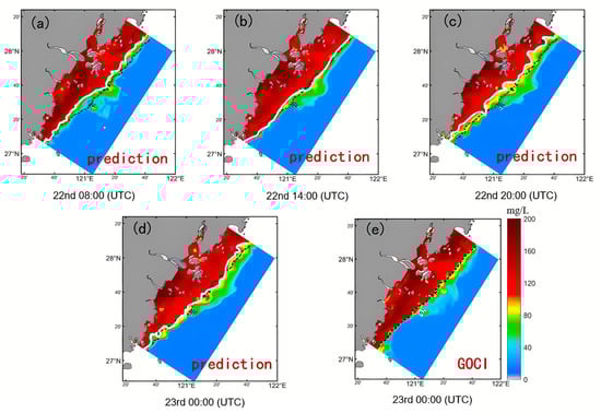
Figure 9. Comparison of SSC 24-h forecast results. 24-h forecast of surface SSC distribution from August 22nd to 23rd. The model outputs for 08:00, 14:00, and 20:00 on the 22nd, followed by 00:00 on the 23rd (UTC), are presented in (a–d). For validation, (e) depicts the GOCI satellite imagery captured at 00:00 on the 23rd. The solid white line tracks the instantaneous predicted 100 mg/L contour. In contrast, the dashed black line marks the fixed observed boundary at the final time step (00:00, 23rd), serving as a static baseline to visualize the movement of the sediment front. Note: While the global RMSE indicates limitations in quantitative precision for long-term forecasts, the visualized contours highlight the model’s capability to capture spatial morphological structures (e.g., the evolution of sediment fronts and plume boundaries), effectively reflecting the relative spatial distribution of the SSC field.

It can be seen that the predicted isoline in Figure 9a–d shows an obvious trend of migrating seaward first, then retreating landward to the nearshore, and subsequently expanding seaward again compared with the remotely observed isoline at 0:00 on the 23rd day, and the time interval of the overall process is about 6 h. This spatial–temporal evolution characteristic is consistent with the law of seaward and landward transport of SSC under the reciprocal action of the tides. Meanwhile, the spatial location of the 100 mg/L SSC isoline predicted at 16 h in Figure 9d is basically the same as that observed by remote sensing at the same time, which indicates that the model is accurate and reliable in predicting the spatial trend of SSC.

4. Conclusions

This study addresses the technical challenge of missing nighttime observations of the suspended sediment concentration (SSC) in coastal waters by integrating hourly GOCI satellite data (2015–2019) for Wenzhou’s coastal waters, high-resolution ERA5 wind fields, and Delft3D hydrodynamic model results. To effectively fill this gap in remote sensing observations, a U-Net deep learning model with multi-source information fusion was developed, providing a novel method for full-cycle SSC estimation. The main results are as follows:

(1)

After the sensitivity analysis of the model parameters, the results show that the addition of tide level information can significantly improve the model’s prediction performance, and the use of the tide level variation instead of the original tide level and the increase in the temporal resolution of the flow field to 15 min can further improve the prediction accuracy of the U-Net model, reducing the average RMSE for 1 h prediction from 39.56 mg/L for S1 to 20.33 mg/L. Meanwhile, the average SSIM of S3 was improved from 0.61 to 0.82, so the model performed better in both prediction accuracy and spatial structure retention.

(2)

The model demonstrates distinct capabilities across different time scales. For short-term predictions, the model achieves high quantitative accuracy. As the forecast horizon extends while point-wise quantitative precision naturally decreases due to error accumulation, the model effectively maintains the global patterns and key spatial features (e.g., sediment fronts). This indicates strong adaptability in capturing the spatial and temporal evolution of SSC, which is attributed to the multi-scale feature fusion of the U-Net structure.

(3)

Despite these accomplishments, the model has certain limitations. As the forecast timeframe is extended to 16 h, quantitative precision naturally decreases due to error accumulation. Consequently, long-term forecasts are most effective at resolving broad concentration categories (e.g., distinguishing high vs. low turbidity zones) rather than providing precise quantitative values.

In addition, errors inherent in preliminary data processing may propagate to the neural network and affect the final accuracy. Due to sample size limitations, only five years of data were used in this study. Since deep learning methods typically perform better with larger datasets [27], future work will therefore focus on expanding the training dataset to further improve the model’s predictive robustness.

References

- Pan, D.; Wang, D. Advances in the Science of Marine Optical Remote Sensing Application in China. Adv. Earth Sci. 2004, 19, 506–512. [Google Scholar] [CrossRef]
- Mao, Z.; Chen, J.; Pan, D.; Tao, B.; Zhu, Q. A regional remote sensing algorithm for total suspended matter in the East China Sea. Remote Sens. Environ. 2012, 124, 819–831. [Google Scholar] [CrossRef]
- Zhan, Y.; Chen, L.; Wang, M.; Wang, D. Determination of Specific Surface Area of Sediment. J. Wuhan Univ. Hydraul. Electr. Eng. 1996, 29, 8–11. [Google Scholar]
- Xiao, Y.; Lu, Q.; Cheng, H.; Zhu, X.; Tang, H. Surface properties of sediments and its effect on phosphorus adsorption. J. Sediment. Res. 2011, 6, 64–68. [Google Scholar] [CrossRef]
- Zhang, J. Heavy metal compositions of suspended sediments in the Changjiang (Yangtze River) estuary: Significance of riverine transport to the ocean. Cont. Shelf Res. 1999, 19, 1521–1543. [Google Scholar] [CrossRef]
- Chen, X.; Shen, H.; Yuan, J.; Li, L. Suspended Sediment Concentration and Fluxes in the High-Turbidity Zone in the Macro-Tidal Hangzhou Bay. J. Mar. Sci. Eng. 2023, 11, 2004. [Google Scholar] [CrossRef]
- Deng, X.; Wang, Z.; Ma, X. Impact of Silted Coastal Port Engineering Construction on Marine Dynamic Environment: A Case Study of Binhai Port. J. Mar. Sci. Eng. 2025, 13, 494. [Google Scholar] [CrossRef]
- Cai, J.; Pan, G.; Chen, P. Analysis of the Characteristics and Dynamic Mechanism of Scouring and Silting Changes in Oufei Tidal Flat Before and After the Reclamation Project. Mar. Sci. Bull. 2020, 39, 63–71. (In Chinese) [Google Scholar] [CrossRef]
- Ying, Z.; Li, N.; Guo, L. Development history and prospects of domestic and international sediment monitoring technology. In Proceedings of the 2023 Academic Annual Conference of Chinese Hydraulic Engineering Society, Zhuzhou, China, 9–10 May 2023; China Water & Power Press: Beijing, China, 2023; pp. 181–186. [Google Scholar]
- Chen, S.; Han, Z.; Li, P. Inversion of suspended sediment concentration and nutrient evaluation in Shanghai offshore waters. Mar. Sci. Bull. 2025, 44, 243–256. [Google Scholar] [CrossRef]
- Winkler, M.K.H.; Bassin, J.P.; Kleerebezem, R.; van der Lans, R.G.J.M.; van Loosdrecht, M.C.M. Temperature and Salt Effects on Settling Velocity in Granular Sludge Technology. Water Res. 2012, 46, 5445–5451. [Google Scholar] [CrossRef]
- Gao, G.D.; Wang, X.; Song, D.; Bao, X.; Yin, B.; Yang, D.; Ding, Y.; Li, H.; Hou, F.; Ren, Z. Effects of wave–current interactions on suspended-sediment dynamics during strong wave events in Jiaozhou Bay, Qingdao, China. J. Phys. Oceanogr. 2018, 48, 1053–1078. [Google Scholar] [CrossRef]
- Yang, X. Study on Hourly Variation of Suspended Sediment Concentration in Coastal Waters of the East China Sea Based on GOCI and Numerical Simulation. Ph.D. Thesis, Shanghai Institute of Technical Physics, Chinese Academy of Sciences, Shanghai, China, 2016. [Google Scholar]
- Xie, J.; Feng, X.; Gao, T.; Wang, Z.; Wan, K.; Yin, B. Application of deep learning in predicting suspended sediment concentration: A case study in Jiaozhou Bay. Mar. Pollut. Bull. 2024, 201, 116255. [Google Scholar] [CrossRef] [PubMed]
- Chen, H.; Gao, X.; Yuan, R. Advances in Remote Sensing and Sensor Technologies for Water-Quality Monitoring: A Review. Water 2025, 17, 3000. [Google Scholar] [CrossRef]
- Li, A.; Yuan, Z.; Guo, Z.; Cheng, Z. A Remote Sensing Retrieval Method for River Water Turbidity Based on a Convolutional Neural Network. J. Geo-Inf. Sci. 2025, 27, 1305–1316. [Google Scholar]
- Sun, X.; Fu, Y.; Han, C.; Fan, Y.; Wang, T. An Inversion Method for Chlorophyll-a Concentration in Global Ocean Through Convolutional Neural Networks. Spectrosc. Spectr. Anal. 2023, 43, 608–613. [Google Scholar] [CrossRef]
- Zhang, H.; Zhou, X.; Tao, Z.; Lv, T.; Wang, J. Deep Learning-Based Turbidity Compensation for Ultraviolet-Visible Spectrum Correction in Monitoring Water Parameters. Front. Environ. Sci. 2022, 10, 986913. [Google Scholar] [CrossRef]
- Mu, J.; Wu, C.; Huang, S. Study on the evolution law of tidal flats in the Oufei Beach sea area of Wenzhou. In Proceedings of the 10th National Academic Symposium on Basic Theory of Sediment, Wuhan, China, 8–11 November 2017; China Water & Power Press: Beijing, China, 2017; pp. 607–611. [Google Scholar] [CrossRef]
- Sun, Y.; Zuo, J.; Zhang, H. Analysis of Variation Characteristics of Suspended Sediment Concentration in Wenzhou Oufei Beach Sea Area. Trans. Oceanol. Limnol. 2016, 3, 28–38. [Google Scholar] [CrossRef]
- Yang, Y.; He, S.; Gu, Y.; Zhu, C.; Wang, L.; Ma, X.; Li, P. Retrieval of Chlorophyll a Concentration Using GOCI Data in Sediment-Laden Turbid Waters of Hangzhou Bay and Adjacent Coastal Waters. J. Mar. Sci. Eng. 2023, 11, 1098. [Google Scholar] [CrossRef]
- He, X.; Bai, Y.; Pan, D.; Huang, N.; Dong, X.; Chen, J.; Chen, C.; Cui, Q. Using geostationary satellite ocean color data to map the diurnal dynamics of suspended particulate matter in coastal waters. Remote Sens. Environ. 2013, 133, 225–239. [Google Scholar] [CrossRef]
- Hu, C. An empirical approach to derive MODIS ocean color patterns under severe sun glint. Geophys. Res. Lett. 2011, 38, L01603. [Google Scholar] [CrossRef]
- Alvera-Azcárate, A.; Barth, A.; Rixen, M.; Beckers, J.M. Reconstruction of incomplete oceanographic data sets using empirical orthogonal functions: Application to the Adriatic Sea surface temperature. Ocean Model. 2005, 9, 325–346. [Google Scholar] [CrossRef]
- Cavalcante, G.H.; Feary, D.A.; Kjerfve, B. Effects of tidal range variability and local morphology on hydrodynamic behavior and salinity structure in the Caeté River Estuary, North Brazil. Int. J. Oceanogr. 2013, 2013, 850579. [Google Scholar] [CrossRef]
- Prairie, Y.T. Evaluating the predictive power of regression models. Can. J. Fish. Aquat. Sci. 1996, 53, 490–492. [Google Scholar] [CrossRef]
- Chen, H.; Lin, X.; Lin, X.Z. Application of Long Short-Term Memory neural network for optimization of numerical simulation results of storm surge. Mar. Forecast. 2024, 41, 1–9. [Google Scholar] [CrossRef]
Disclaimer/Publisher’s Note: The statements, opinions and data contained in all publications are solely those of the individual author(s) and contributor(s) and not of MDPI and/or the editor(s). MDPI and/or the editor(s) disclaim responsibility for any injury to people or property resulting from any ideas, methods, instructions or products referred to in the content. |
© 2026 by the authors. Licensee MDPI, Basel, Switzerland. This article is an open access article distributed under the terms and conditions of the Creative Commons Attribution (CC BY) license.