On Swarm-Constrained Formation Tracking Control Method for Master–Slave AUVs with Dynamic Transformations

Abstract

Aiming at the problem of complex cluster constraints in the process of master slave AUV (Autonomous Underwater Vehicle) formation transformation and tracking in the wave environment, it is proposed to introduce the model predictive control (MPC) method to normalize a variety of complex constraints in the process of group formation navigation, unify the kinematic model and dynamic model, and introduce the normalized constraint equation. At the same time, the MPC formation transformation tracking control strategy is designed to achieve AUV formation transformation and tracking control under the unified model, which is verified through simulation tests to provide more effective technical support for AUV group formation.

1. Introduction

With the development of marine resource exploration and the challenge of the coastal defense situation, the area of marine use is heading for the deep sea. As they are main equipment for marine environmental monitoring, resource exploration, and marine search and rescue, demand for AUVs (Autonomous Underwater Vehicles) in ocean-going sea areas is increasing, especially the formation application under the multi-body/swarm, which has become highlighted in research [1,2,3].

In most domestic and international studies on formation control of AUV clusters, AUVs are typically treated as point masses in formation control purposes [4]. Furthermore, the majority of computer simulation research primarily considers the kinematic models of AUVs, while failing to incorporate crucial constraints such as dynamic models, inherent operational limitations of the vehicles, and external environmental disturbances as constraints for swarm formation. These idealized research conditions deviate significantly from real-world scenarios, resulting in substantial discrepancies between theoretical models and practical applications.

In tracking control research, Xu J. and Wang M. et al. appropriately constructed a backstepping method [5,6] and replaced the terms causing singular values for spatial trajectory tracking of underactuated AUVs. By using a velocity control method instead of attitude control, singularity problems, which were commonly found in general backstepping methods, were avoided effectively. In addition, Raja R. et al. proposed a backstepping approach for the formation control of multiple leader–follower AUVs, in terms of constraints; paper [7] only considers environmental disturbances and obstacle interference, but does not account for the AUV’s own constraints and the constraints among the cluster of AUVs. Chen X. provides an adaptive sliding mode path following a control system [8] for USVs under the influence of ocean currents; however, state constraints and the AUV’s own inherent limitations remain unaddressed in the path-following control scheme. A swarm decentralized formation cooperative control method is provided for AUV homing in paper [9]; in terms of controller design and constraint analysis, the study addresses the docking sequence and positional constraints within the AUV cluster, as well as ocean current disturbances, during the recovery process. However, these constraints are not effectively incorporated into the control law. Furthermore, the inherent physical constraints of individual AUVs are not accounted for. Consequently, the simulation results appear relatively idealized compared to real-world conditions. Aiming at the problems of high communication pressure and information redundancy of the multi-AUV system in the marine environment, paper [10] adopts a distributed event-triggered formation control method via asynchronous periodic sampling control approach, which realizes the discrete leaderless multi-AUV distributed event-triggered formation control. However, the study simplifies AUVs as point masses for swarm planning. Moreover, the controller design does not incorporate the dynamic model and relies solely on a kinematic framework. Consequently, the analytical results may deviate from the actual motion characteristics of real AUVs. A fixed-time sliding control scheme is developed for AUV tracking control in paper [11] under model parameter uncertainties and external disturbances (the wind, waves, and ocean currents). This study fails to account for the vehicle’s inherent constraints, state constraints, and proximity constraints.

Analyzing the state of the art of AUV tracking control and related control methods overall, there are still limitations in research such as theoretical emphasis, inadequate constraints being considered, and insufficient control accuracy. And the difficult problems of the moving base AUV tracking research are analyzed in combination with various complex constraints on, and interferences with, the tracking process.

Due to its strong performance in handling control problems with multiple constraints, multiple variables, and uncertainties, the Model Predictive Control (MPC) method [12,13,14] is introduced in this paper for the algorithm design of AUV formation tracking control. To address issues such as underactuation, nonholonomic constraints, and model nonlinearity in AUV tracking control, Zhang Wei et al. designed a nonlinear continuous MPC tracking controller [15,16,17,18]. Through simulations, the effectiveness of this controller in AUV vertical plane control was demonstrated, and its performance was further verified via simple trapezoidal tracking experiments in the vertical plane. A robust model predictive control (MPC) framework based on the implementation of the receding horizon is implemented to address the challenges of unknown external disturbances and model uncertainties faced by the AUV in trajectory tracking control [19]. This article demonstrates a marked increase in the consideration of constraints compared to prior research, encompassing not only model uncertainties and environmental constraints but also the AUV’s own limitations. However, a notable limitation is that the reference trajectory is generated by a predefined function rather than being autonomously produced by the AUV under control inputs. Zhang Y. and Liu X. et al. [20] transformed trajectory tracking control into a constrained optimization problem, fully considering ocean current disturbances and state constraints. They designed a constrained optimization algorithm based on standard convex quadratic programming for AUV 3D trajectory tracking control. Simulation-based tracking verification on different trajectories demonstrated the robustness and feasibility of the proposed underwater trajectory tracking algorithm.

Current research on AUV tracking and swarm tracking mainly faces the following issues:

(1)

Insufficient consideration of constraint conditions during swarm tracking analysis. Most studies focus only on environmental disturbances, neglecting other complex constraints such as state constraints, inherent limitations, and proximity constraints. Some research considers two types of constraints but handles them separately with independent restrictions, rather than integrating them through normalized treatment to form a unified constraint framework for investigation.

(2)

Oversimplification of AUV dynamics in most studies. AUVs are often modeled as point masses in simulations, failing to adequately account for their inherent physical limitations, such as thruster speed, turning radius, and maximum rudder angles. This leads to significant discrepancies between simulation results and actual performance.

(3)

Unrealistic trajectory assumptions in tracking studies. Most research employs predefined trajectories—such as straight lines, sinusoidal curves, circular paths, or 3D spirals—rather than using actual trajectories generated by the autonomous navigation of a leader AUV. Consequently, some predefined trajectories may contradict the AUV’s actual motion capabilities, rendering them infeasible in practice.

To address the multiple complex constraints in the process of AUV cluster formation transformation and tracking—including state constraints, collision avoidance and proximity constraints, inherent constraints, and environmental disturbance constraints—this study first analyzes and represents these constraints as follows: state constraints are defined as restrictions on the heading and pitch angles of the follower AUVs based on the opening angle of their detection sensors; inherent constraints include thruster speed limits, turning radius limits, and rudder angle limits; environmental disturbance constraints refer to ocean current interference; and collision avoidance and proximity constraints are characterized as interaction force constraints arising from close distances between AUVs.

Subsequently, the model predictive control (MPC) method is introduced to process and convert these constraints into state constraints, output constraints, and control input constraints of the predictive model. An MPC normalization approach is then applied to unify all constraints into control input increment constraints. Next, the continuous AUV model is discretized, and an error-augmented model for the AUV is derived using the MPC framework. A formation transformation tracking objective optimization function is designed, incorporating the aforementioned constraints. By solving this function, control input increments are obtained, which are then used to generate new control inputs for the follower AUVs to track the leader AUV. Throughout this process, a segmented formation transformation function is designed based on trajectory data generated by the leader AUV under control actions, enabling the follower AUVs to automatically track the leader’s formation changes. A series of numerical simulations are designed to validate the approach, including two follower AUVs tracking the leader on the horizontal plane; two followers tracking while transforming formations on the horizontal plane; two followers tracking and transforming formations in three-dimensional space; and six followers tracking and transforming formations in three-dimensional space. In the second operational scenario, a comparative simulation with traditional PID control is conducted. Finally, the designed tracking control method is adapted and applied to a pool experiment involving a single AUV tracking a moving target.

2. AUV Swarm Formation Model

By integrating and unifying the kinematic and dynamic models, the resulting spatial model is derived as follows [12]:

$$\left\{\begin{array}{l}\dot{\mathit{\eta }}=\mathit{J}\left(\mathit{\eta }\right)\mathit{\nu }\\ \mathit{M}\dot{\mathit{\nu }}+\mathit{C}\left(\mathit{\nu }\right)\mathit{\nu }+\mathit{D}\left(\mathit{\nu }\right)\mathit{\nu }=\mathit{\tau }\end{array}\right.$$

(1)

where the position and posture information is $\mathit{\eta }={\left[\begin{array}{cccccc}\xi & \eta & \zeta & \phi & \theta & \psi \end{array}\right]}^{\mathrm{T}}$, the speed is $\mathit{\nu }={\left[\begin{array}{cccccc}u& v& w& p& q& r\end{array}\right]}^{\mathrm{T}}$, the control amount is $\mathit{\tau }={\left[\begin{array}{cccccc}{\tau }_u& {\tau }_v& {\tau }_w& {\tau }_p& {\tau }_q& {\tau }_r\end{array}\right]}^{\mathrm{T}}$, and the coordinate transformation matrix is

$$\mathit{J}=\left[\begin{array}{cccccc}\cos \psi \cos \theta & -\sin \psi \cos \phi +\sin \phi \sin \theta \cos \psi & \sin \psi \sin \phi +\sin \theta \cos \psi \cos \phi & 0& 0& 0\\ \sin \psi \cos \theta & \cos \psi \cos \phi +\sin \phi \sin \theta \sin \psi & -\cos \psi \sin \phi +\sin \theta \sin \psi \cos \phi & 0& 0& 0\\ -\sin \theta & \sin \phi \cos \theta & \cos \phi \cos \theta & 0& 0& 0\\ 0& 0& 0& 1& \sin \phi \tan \theta & \cos \phi \tan \theta \\ 0& 0& 0& 0& \cos \phi & -\sin \phi \\ 0& 0& 0& 0& \sin \phi /\cos \theta & \cos \phi /\cos \theta \end{array}\right]$$

The positive definite inertia matrix is composed of the mass and moment of the inertia matrix and the added mass matrix:

$$\mathit{M}={\mathit{M}}_{\mathit{R}\mathit{B}}+{\mathit{M}}_{\mathit{A}}=\left[\begin{array}{cccccc}m-X_{\dot{u}}& 0& 0& 0& 0& 0\\ 0& m-Y_{\dot{v}}& 0& 0& 0& 0\\ 0& 0& m-Z_{\dot{w}}& 0& 0& 0\\ 0& 0& 0& I_x-K_{\dot{p}}& 0& 0\\ 0& 0& 0& 0& I_y-M_{\dot{q}}& 0\\ 0& 0& 0& 0& 0& I_z-N_{\dot{r}}\end{array}\right];$$

The centripetal force matrix is composed of the centripetal force matrix of the intelligent ship and the Coriolis centripetal matrix generated by the added mass:

$$\mathit{C}={\mathit{C}}_{\mathit{R}\mathit{B}}+{\mathit{C}}_{\mathit{A}}=\left[\begin{array}{cccccc}0& 0& 0& 0& mw-Z_{\dot{w}}w& -mv+Y_{\dot{v}}v\\ 0& 0& 0& -mw+Z_{\dot{w}}w& 0& mu-X_{\dot{u}}u\\ 0& 0& 0& mv-Y_{\dot{v}}v& -mu+X_{\dot{u}}u& 0\\ 0& mw-Z_{\dot{w}}w& -mv+Y_{\dot{v}}v& 0& I_{z}r-N_{\dot{r}}r& -I_{y}q+M_{\dot{q}}q\\ -mw+Z_{\dot{w}}w& 0& mu-X_{\dot{u}}u& -I_{z}r+N_{\dot{r}}r& 0& I_{x}p-K_{\dot{p}}p\\ mv-Y_{\dot{v}}v& -mu+X_{\dot{u}}u& 0& I_{y}q-M_{\dot{q}}q& -I_{x}p+K_{\dot{p}}p& 0\end{array}\right];$$

The fluid damping force matrix includes the first-order damping force and moment and the second-order damping force and moment:

$$\mathit{D}=-diag\left\{X_u,Y_v,Z_w,K_p,M_q,N_r\right\}-diag\left\{X_{\left|u\right|u}\left|u\right|,Y_{\left|v\right|v}\left|v\right|,Z_{\left|w\right|w}\left|w\right|,K_{\left|p\right|p}\left|p\right|,M_{\left|q\right|q}\left|q\right|,N_{\left|r\right|r}\left|r\right|\right\};$$

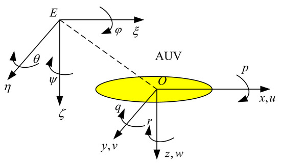
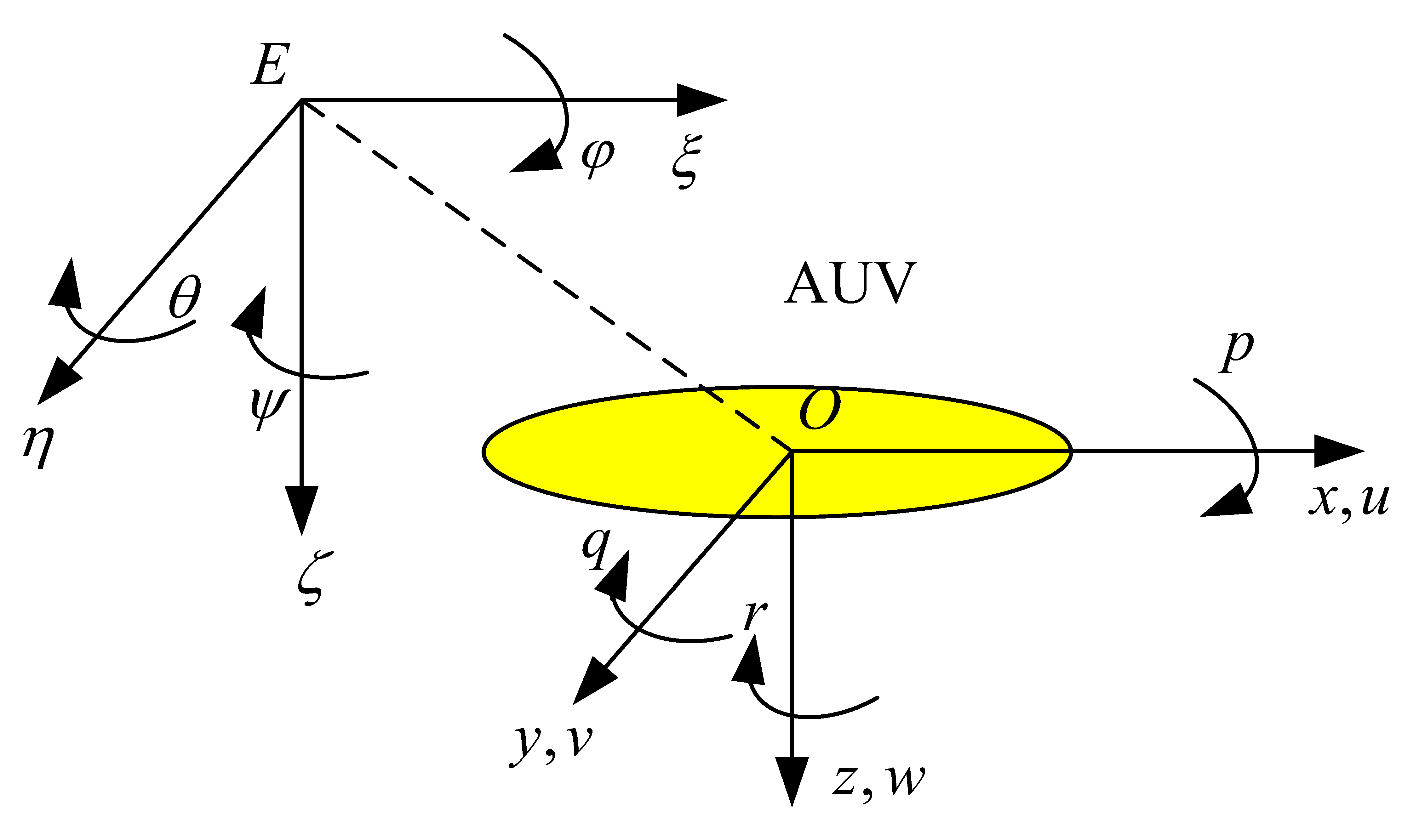
where $x,y,z$ are the surge, sway, and heave displacement in the motion coordinate system; $\xi ,\eta ,\zeta$ are the north, east, and depth displacement in the fixed coordinate system; $\phi ,\theta ,\psi$ are the angle of roll, pitch, and yaw; $u,v,w,p,q,r$ are the speed of surge, sway, heave, roll, pitch, and yaw; ${\tau }_u,{\tau }_v,{\tau }_w,{\tau }_p,{\tau }_q,{\tau }_r$ are the control force and moment of surge, sway, heave, roll, pitch, and yaw; $m$ is the mass of the AUV; $X_{(•)},Y_{(•)},Z_{(•)},K_{(•)},M_{(•)},N_{(•)}$ are the hydrodynamic derivatives; $I_x,I_y,I_z$ are the moments of inertia.

Each AUV in the formation establishes its own spatial motion model according to the method described above. The coordinate system of the AUV is shown in the Figure 1 below.

Figure 1. Fixed coordinate system and motion coordinate system.

3. Complex Constraint Normalization Processing

By analyzing the disturbances and limitations faced by the AUV swarm during formation navigation, these issues are categorized into four types: state constraints, self-imposed constraints, disturbance constraints, and proximity constraints [13].

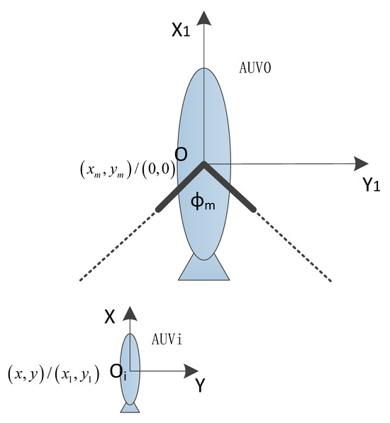
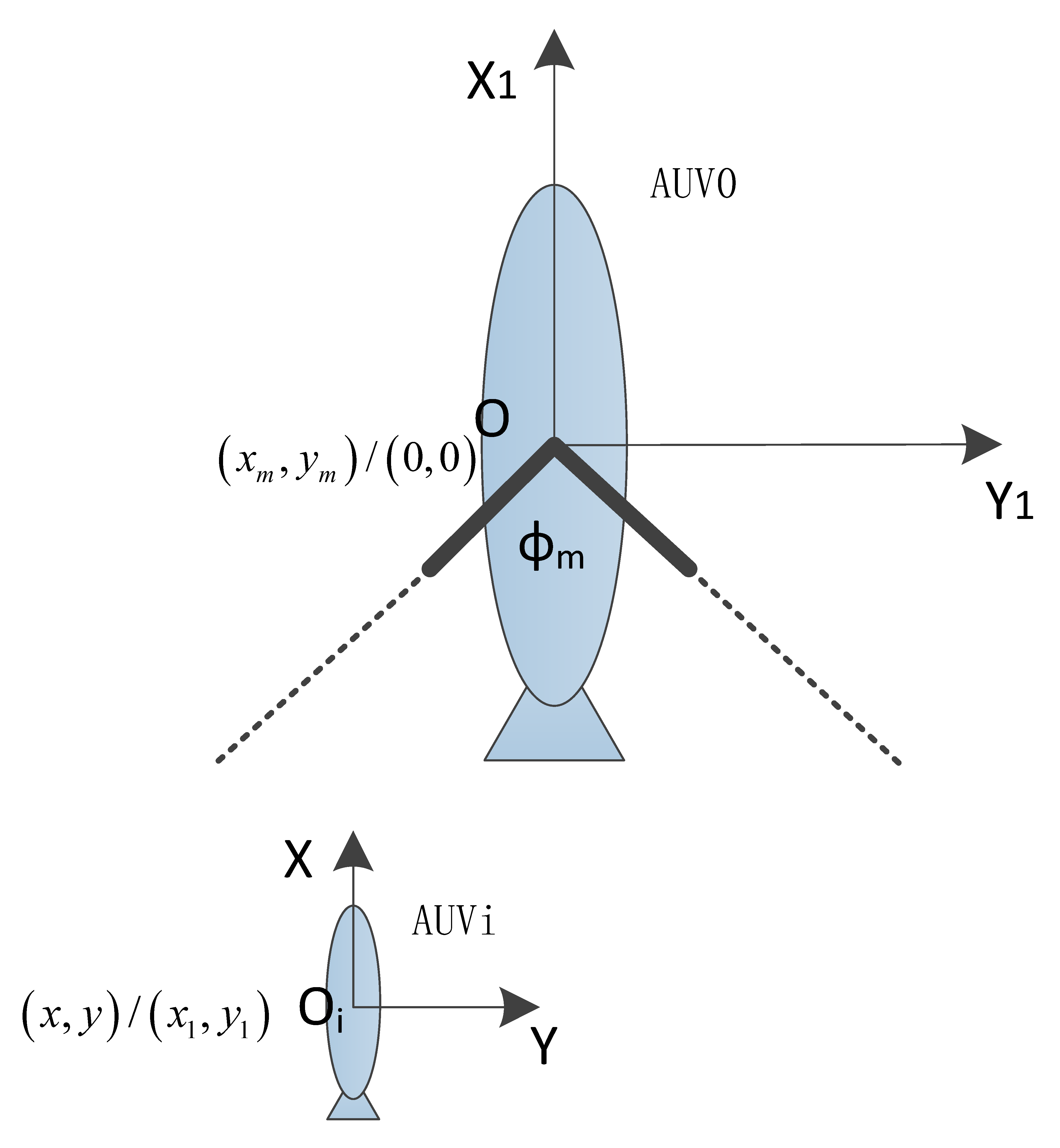
State constraints refer to the restrictions imposed on the heading of the AUV, primarily for tracking direction constraints. The guidance sensors mounted on the lead vehicle must be within the detection range of the tracking sensors on the follower vessels to ensure stable guidance signals during tracking, which requires appropriate heading and position of the AUVs (Figure 2).

$$-{\displaystyle \frac{1}{2}}{\mathrm{\Phi }}_m<\arctan {\displaystyle \frac{e_y}{e_x}}<{\displaystyle \frac{1}{2}}{\mathrm{\Phi }}_m$$

(2)

where $e_x=x_m-x$ and $e_y=y_m-y$ represent the relative positional distance between the master and slave AUVs in the motion coordinate system, $\left(x_m,y_m\right)$ denotes the position coordinates of the master in the moving coordinate system, $\left(x,y\right)$ indicates the position coordinates of the slave AUVs in the motion coordinate system, and ${\mathrm{\Phi }}_m$ is the detection angle of the sensor installed on the AUV; the range of ${\mathrm{\Phi }}_m$ is typically within ±60 degrees,. According to Equation (2), the constraint of the surge error on the sway error can be derived as follows.

$$y_m+\left(x_m-x\right)\tan ({\displaystyle \frac{1}{2}}{\mathrm{\Phi }}_m)<y<y_m-\left(x_m-x\right)\tan ({\displaystyle \frac{1}{2}}{\mathrm{\Phi }}_m)$$

(3)

Figure 2. Division of safe recovery zone and restricted entry zone for mother ship.

Subsequently, this position constraint in the motion coordinate system is transformed into the fixed coordinate system.

$$\left(\xi ,\eta ,\zeta \right)={{\mathit{J}}_{3\times 3}}^{-1}\left(x,y,z\right)$$

(4)

Thus, the output constraint is obtained.

Self-imposed constraints mainly arise from the limitations of the actuators equipped on the AUVs, such as thruster speed and rudder angle. These are ultimately translated into restrictions on rudder angle and thrust magnitude.

$$\left\{\begin{array}{c}-{\delta }_{r\max }\le {\delta }_r\le {\delta }_{r\max }\\ -{\delta }_{q\max }\le {\delta }_q\le {\delta }_{q\max }\\ -{\tau }_{r\max }\le {\tau }_r\le {\tau }_{r\max }\\ -{\tau }_{q\max }\le {\tau }_q\le {\tau }_{q\max }\\ -{\tau }_{u\max }\le {\tau }_u\le {\tau }_{u\max }\end{array}\right.$$

(5)

where ${\delta }_r$ is the rudder angle, the range of the rudder angle is typically within ±30 degrees, ${\delta }_q$ is the elevator angle, the range of the rudder angle is typically within ±30 degrees, ${\tau }_u$ is the surge thrust, ${\tau }_q$ is the pitch moment, and ${\tau }_r$ is the yaw moment.

Disturbance constraints primarily involve environmental perturbations. Assuming the magnitude of this disturbance is ${\tau }_d$ and its direction in the earth-fixed coordinate system is ${\psi }_d$, then in the earth-fixed coordinate system, this disturbance can be decomposed in the horizontal plane as shown below.

$${\left[\begin{array}{cc}{\tau }_d\cos {\psi }_d& {\tau }_d\sin {\psi }_d\end{array}\right]}^T$$

(6)

Proximity constraints refer to the interference caused when two or more AUVs approach each other during formation changes. This interference is mainly manifested as sway force disturbances on the AUVs, with the magnitude of the force increasing as the distance between the AUVs decreases.

$$-{\tau }_{f\max }\le {\tau }_{vf}=f\left(\mathrm{\Delta }l\right)\le {\tau }_{f\max }$$

(7)

where ${\tau }_{vf}$ represents the sway interference force, $\mathrm{\Delta }l$ is the sway distance between the two vessels, and ${\tau }_{f\max }$ denotes the maximum value of the sway interference force; the magnitude of this value depends on both the size of the two AUVs and the distance between them.

The MPC method is employed to unify these complex constraints into constraints on control inputs and their increments, achieving normalized processing.

4. Formation Transformation Tracking Control Algorithm

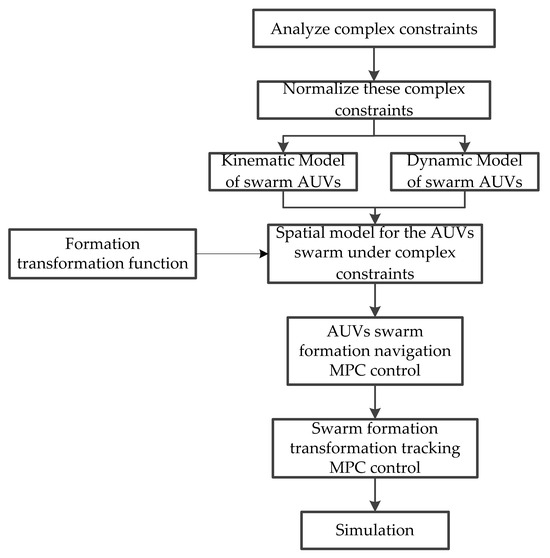
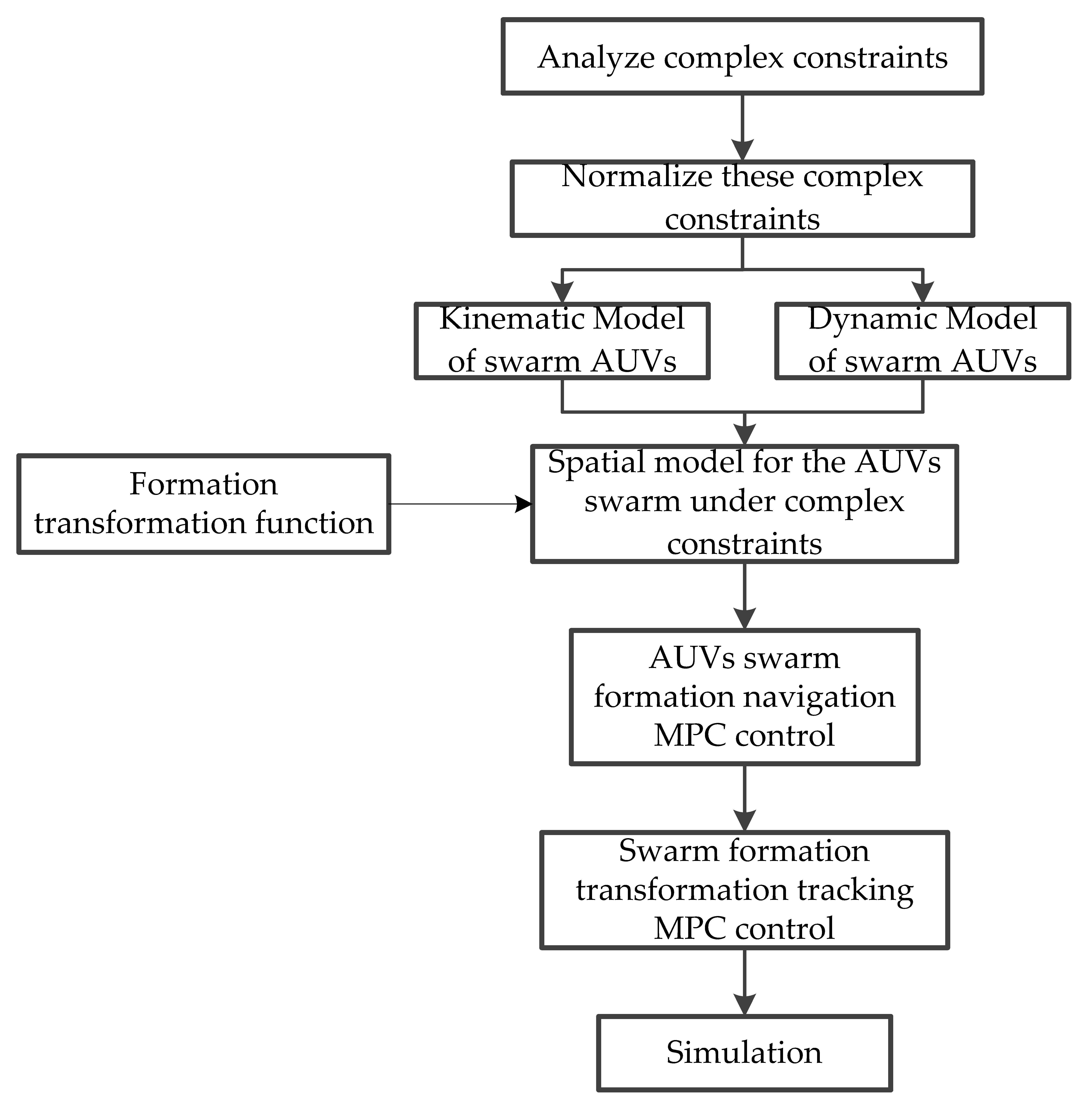
The design logic of the formation transformation tracking control algorithm for master–slave AUVs is as follows (Figure 3):

Figure 3. The design logic of the formation transformation tracking control algorithm.

(1)

Analyze the diverse complex constraints during AUV swarm formation navigation;

(2)

Apply the MPC method to normalize these complex constraints;

(3)

Integrate the kinematic and dynamic models, incorporate normalized constraints, and construct a spatial model for the AUV swarm under complex constraints;

(4)

Design an MPC-based control method for AUV swarm formation navigation. By introducing a formation transformation function, propose an MPC-based AUV swarm formation transformation tracking method to address complex constraints and dynamic effects in simulation environments.

4.1. Master AUV Controller

Unlike the conventional master AUV trajectory that only considers the kinematic model and artificially gives the motion trajectory, in this paper, the master AUV navigation is designed according to the dynamic model and kinematic model, and different constant control quantities are designed in different time periods, so that the master AUV can change the navigational position and attitude according to the 3-dimensional control quantity, and form a leading trajectory.

$${\mathit{\tau }}_0=\left\{\begin{array}{c}{\left[\begin{array}{cccccc}{\tau }_{u0}& {\tau }_{v0}& {\tau }_{w0}& {\tau }_{p0}& {\tau }_{q0}& {\tau }_{r0}\end{array}\right]}^{\mathrm{T}}, t\in [0,t_1)\\ {\left[\begin{array}{cccccc}{\tau }_{u1}& {\tau }_{v1}& {\tau }_{w1}& {\tau }_{p1}& {\tau }_{q1}& {\tau }_{r1}\end{array}\right]}^{\mathrm{T}}, t\in [t_1,t_2)\\ {\left[\begin{array}{cccccc}{\tau }_{u2}& {\tau }_{v2}& {\tau }_{w2}& {\tau }_{p2}& {\tau }_{q2}& {\tau }_{r2}\end{array}\right]}^{\mathrm{T}}, t\in [t_2,t_3]\end{array}\right.$$

(8)

4.2. Slave AUV Controller

Firstly, the AUV model will be discretized and rewritten into an error-augmented model following the model predictive control method. The AUV formation transformation control mainly deals with the control of the AUV position and attitude, and the tracking controller is designed using the model predictive control (MPC) method, where the state quantity, speed quantity, and output quantity are all 6-DOF [14].

$$\left\{\begin{array}{l}{\dot{\mathit{x}}}_1={\mathit{A}}_{1c}{\mathit{x}}_1+{\mathit{B}}_{1c}\left({\mathit{u}}_1+{\mathit{d}}_{1u}\right)\\ {\mathit{y}}_1={\mathit{C}}_{1c}{\mathit{x}}_1\end{array}\right.$$

(9)

where the state variable is ${\mathit{x}}_1={\left[u,v,w,p,q,r,\xi ,\eta ,\zeta ,\phi ,\theta ,\psi \right]}^{\mathrm{T}}$, the control variable is ${\mathit{u}}_1={\left[{\tau }_u,{\tau }_v,{\tau }_w,{\tau }_p,{\tau }_q,{\tau }_r\right]}^{\mathrm{T}}$, the output is ${\mathit{y}}_1={\left[\xi ,\eta ,\zeta ,\phi ,\theta ,\psi \right]}^{\mathrm{T}}$, the coefficient matrices are ${\mathit{A}}_{1c}=\left[\begin{array}{cc}-{\mathit{M}}^{-1}\mathit{C}-{\mathit{M}}^{-1}\mathit{D}& {\mathsf{0}}_{6\times 6}\\ \mathit{J}& {\mathsf{0}}_{6\times 6}\end{array}\right]$, ${\mathit{B}}_{1c}=\left[\begin{array}{c}{\mathit{M}}^{-1}\\ {\mathsf{0}}_{6\times 6}\end{array}\right]$, ${\mathit{C}}_{1c}=\left[\begin{array}{cc}{\mathsf{0}}_{6\times 6}& {\mathit{I}}_{6\times 6}\end{array}\right]$; and the interference variable is ${\mathit{d}}_{1u}$; it mainly refers to the 6-DOF disturbance quantity obtained. B. decomposing the current disturbance in the AUV motion coordinate system, in which the current disturbance is set as a disturbance force with fixed direction and magnitude in the fixed coordinate system.

The continuous model is discretized into the following model. The discretization method is a zero-order hold method and the sampling time Ts is 1 s.

The motion dynamics of an AUV are typically a “slow” process, with time constants for changes in speed and heading generally on the order of several to tens of seconds. A sampling period of 1 s is sufficient to capture these primary dynamic changes, meeting the basic requirements of the Shannon sampling theorem. Model Predictive Control (MPC) requires solving an optimization problem online within each sampling period. A Ts = 1 s provides ample computation time for the solver (e.g., completing the calculation within a few hundred milliseconds), ensuring that the controller can output control signals before the next cycle, thereby meeting the demands of real-time control. If Ts is too small, the discrete model becomes more accurate and closer to the continuous system, but the computational load increases dramatically. This may also lead to numerically ill-conditioned system matrices after discretization, making real-time implementation difficult. Conversely, if Ts is too large, the computational burden is reduced, improving operational efficiency, but the overly large step size tends to miss information about dynamic changes in the system. This can result in instability of the discrete system, noticeable oscillations, and larger tracking errors. Therefore, Ts = 1 s was chosen for model discretization after extensive testing.

$$\left\{\begin{array}{l}{\mathit{x}}_1(k+1)={\mathit{A}}_{1p}{\mathit{x}}_1(k)+{\mathit{B}}_{1p}\left({\mathit{u}}_1(k)+{\mathit{d}}_{1u}(k)\right)\\ {\mathit{y}}_1(k)={\mathit{C}}_{1p}{\mathit{x}}_1(k)\end{array}\right.$$

(10)

where ${\mathit{x}}_1\left(k\right),{\mathit{u}}_1\left(k\right),{\mathit{y}}_1\left(k\right),{\mathit{d}}_{1u}(k)$ are the state variable, control variable, output variable, and interference variable at time k; $\mathit{x}\left(k+1\right)$ is the state variable at time k + 1; ${\mathit{A}}_{1p},{\mathit{B}}_{1p},{\mathit{C}}_{1p}$ are the coefficient matrices of the discrete model.

Then, a prediction model is constructed based on the discrete model.

From discrete model (10), $\left\{\begin{array}{l}{\mathit{x}}_1\left(k+1\right)={\mathit{A}}_{1p}{\mathit{x}}_1\left(k\right)+{\mathit{B}}_{1p}\left({\mathit{u}}_1(k)+{\mathit{d}}_{1u}(k)\right)\\ {\mathit{x}}_1\left(k\right)={\mathit{A}}_{1p}{\mathit{x}}_1\left(k-1\right)+{\mathit{B}}_{1p}\left({\mathit{u}}_1(k-1)+{\mathit{d}}_{1u}(k-1)\right)\end{array}\right.$.

Subtracting the two equations yields the following equation.

$${\mathit{x}}_1\left(k+1\right)-{\mathit{x}}_1\left(k\right)={\mathit{A}}_{1p}\left({\mathit{x}}_1\left(k\right)-{\mathit{x}}_1\left(k-1\right)\right)+{\mathit{B}}_{1p}\left(\left({\mathit{u}}_1\left(k\right)-{\mathit{u}}_1\left(k-1\right)\right)+\left({\mathit{d}}_{1u}(k)-{\mathit{d}}_{1u}(k-1)\right)\right)$$

(11)

Setting the $\mathrm{\Delta }{\mathit{x}}_1\left(k+1\right)={\mathit{x}}_1\left(k+1\right)-{\mathit{x}}_1\left(k\right)$, $\mathrm{\Delta }{\mathit{x}}_1\left(k\right)={\mathit{x}}_1\left(k\right)-{\mathit{x}}_1\left(k-1\right)$, $\mathrm{\Delta }{\mathit{u}}_1\left(k\right)={\mathit{u}}_1\left(k\right)-{\mathit{u}}_1\left(k-1\right)$, $\mathrm{\Delta }{\mathit{d}}_{1u}(k)={\mathit{d}}_{1u}(k)-{\mathit{d}}_{1u}(k-1)$, the error state-space equation is shown as follows,

$$\mathrm{\Delta }{\mathit{x}}_1\left(k+1\right)={\mathit{A}}_{1p}\mathrm{\Delta }{\mathit{x}}_1\left(k\right)+{\mathit{B}}_{1p}(\mathrm{\Delta }{\mathit{u}}_1\left(k\right)+\mathrm{\Delta }{\mathit{d}}_{1u}\left(k\right))$$

(12)

where $\mathrm{\Delta }{\mathit{x}}_1\left(k+1\right)=\left[\begin{array}{c}u\left(k+1\right)-u\left(k\right)\\ v\left(k+1\right)-v\left(k\right)\\ w\left(k+1\right)-w\left(k\right)\\ p\left(k+1\right)-p\left(k\right)\\ q\left(k+1\right)-q\left(k\right)\\ r\left(k+1\right)-r\left(k\right)\\ \xi \left(k+1\right)-\xi \left(k\right)\\ \eta \left(k+1\right)-\eta \left(k\right)\\ \zeta \left(k+1\right)-\zeta \left(k\right)\\ \phi \left(k+1\right)-\phi \left(k\right)\\ \theta \left(k+1\right)-\theta \left(k\right)\\ \psi \left(k+1\right)-\psi \left(k\right)\end{array}\right]$, $\mathrm{\Delta }{\mathit{u}}_1\left(k\right)=\left[\begin{array}{c}{\tau }_u\left(k\right)-{\tau }_u\left(k-1\right)\\ {\tau }_v\left(k\right)-{\tau }_v\left(k-1\right)\\ {\tau }_w\left(k\right)-{\tau }_w\left(k-1\right)\\ {\tau }_p\left(k\right)-{\tau }_p\left(k-1\right)\\ {\tau }_q\left(k\right)-{\tau }_q\left(k-1\right)\\ {\tau }_r\left(k\right)-{\tau }_r\left(k-1\right)\end{array}\right]$.

Next, combine the error states $\mathrm{\Delta }\mathit{x}\left(k\right)$ and output $y\left(k\right)$ to construct a new state error vector ${\mathit{x}}_e\left(k\right)={\left[\begin{array}{cc}\mathrm{\Delta }\mathit{x}{\left(k\right)}^{\mathrm{T}}& \mathit{y}\left(k\right)\end{array}\right]}^{\mathrm{T}}$, subtracting the output at times k and k + 1,

$${\mathit{y}}_1\left(k+1\right)-{\mathit{y}}_1\left(k\right)={\mathit{C}}_{1p}{\mathit{x}}_1\left(k+1\right)-{\mathit{C}}_{1p}{\mathit{x}}_1\left(k\right)={\mathit{C}}_{1p}\mathrm{\Delta }{\mathit{x}}_1\left(k+1\right)$$

(13)

Putting (11) into (12),

$${\mathit{y}}_1\left(k+1\right)={\mathit{C}}_{1p}{\mathit{A}}_{1p}\mathrm{\Delta }{\mathit{x}}_1\left(k\right)+{\mathit{y}}_1\left(k\right)+{\mathit{C}}_{1p}{\mathit{B}}_{1p}(\mathrm{\Delta }{\mathit{u}}_1\left(k\right)+\mathrm{\Delta }{\mathit{d}}_{1u}\left(k\right))$$

(14)

So, the error-augmented model is as follows,

$$\left\{\begin{array}{l}\left[\begin{array}{c}\mathrm{\Delta }{\mathit{x}}_1{\left(k+1\right)}^{\mathrm{T}}\\ {\mathit{y}}_1\left(k+1\right)\end{array}\right]=\left[\begin{array}{cc}{\mathit{A}}_{1p}& {\mathsf{0}}_{12\times 6}\\ {\mathit{C}}_{1p}{\mathit{A}}_{1p}& {\mathit{I}}_{6\times 6}\end{array}\right]\left[\begin{array}{c}\mathrm{\Delta }{\mathit{x}}_1{\left(k\right)}^{\mathrm{T}}\\ {\mathit{y}}_1\left(k\right)\end{array}\right]+\left[\begin{array}{c}{\mathit{B}}_{1p}\\ {\mathit{C}}_{1p}{\mathit{B}}_{1p}\end{array}\right](\mathrm{\Delta }{\mathit{u}}_1\left(k\right)+\mathrm{\Delta }{\mathit{d}}_{1u}(k))\\ {\mathit{y}}_1\left(k\right)=\left[\begin{array}{cc}{\mathsf{0}}_{6\times 12}& {\mathit{I}}_{6\times 6}\end{array}\right]\left[\begin{array}{c}\mathrm{\Delta }{\mathit{x}}_1{\left(k\right)}^{\mathrm{T}}\\ {\mathit{y}}_1\left(k\right)\end{array}\right]\end{array}\right.$$

(15)

then transformed into the following discrete error-augmented model.

$$\left\{\begin{array}{l}{\mathit{x}}_{1e}\left(k+1\right)={\mathit{A}}_{1e}{\mathit{x}}_{1e}\left(k\right)+{\mathit{B}}_{1e}\left({\mathit{u}}_{1e}\left(k\right)+{\mathit{d}}_{1ue}\left(k\right)\right)\\ {\mathit{y}}_{1e}\left(k\right)={\mathit{C}}_{1e}{\mathit{x}}_{1e}\left(k\right)\end{array}\right.$$

(16)

where the state variable is ${\mathit{x}}_{1e}\left(k\right)={\left[\begin{array}{cc}\mathrm{\Delta }{\mathit{x}}_1{\left(k\right)}^{\mathrm{T}}& {\mathit{y}}_1\left(k\right)\end{array}\right]}^{\mathrm{T}}$ at time $k$, the state variable is ${\mathit{x}}_{1e}\left(k+1\right)={\left[\begin{array}{cc}\mathrm{\Delta }{\mathit{x}}_1{\left(k+1\right)}^{\mathrm{T}}& {\mathit{y}}_1\left(k+1\right)\end{array}\right]}^{\mathrm{T}}$ at time $k+1$, the control variable is ${\mathit{u}}_{1e}\left(k\right)=\mathrm{\Delta }{\mathit{u}}_1\left(k\right)$ at time $k$, the interference variable is ${\mathit{d}}_{1ue}\left(k\right)=\mathrm{\Delta }{\mathit{d}}_{1u}\left(k\right)$ at time $k$, the output is ${\mathit{y}}_{1e}\left(k\right)$ at time $k$, ${\mathit{A}}_{1e}, {\mathit{B}}_{1e}, {\mathit{C}}_{1e}$ are the coefficient matrices of the prediction model, ${\mathit{A}}_{1e}=\left[\begin{array}{cc}{\mathit{A}}_{1p}& {\mathsf{0}}_{12\times 6}\\ {\mathit{C}}_{1p}{\mathit{A}}_{1p}& {\mathit{I}}_{6\times 6}\end{array}\right]$, ${\mathit{B}}_{1e}=\left[\begin{array}{c}{\mathit{B}}_{1p}\\ {\mathit{C}}_{1p}{\mathit{B}}_{1p}\end{array}\right]$, ${\mathit{C}}_{1e}=\left[\begin{array}{cc}{\mathsf{0}}_{6\times 12}& {\mathit{I}}_{6\times 6}\end{array}\right]$ where ${\mathit{A}}_{1p}$, ${\mathit{B}}_{1p}$, and ${\mathit{C}}_{1p}$ are the coefficient matrices after discretization.

Expand the above error enhancement model in the prediction time domain and the control time domain, and arrange it to obtain a prediction model of the AUV.

Set the prediction horizon of MPC as $N_p$, the control horizon as $N_c$, and the current time step as $k$. Denote the predicted states over the prediction horizon as ${\mathit{x}}_{1e}\left(\left.k+1\right|k\right)$, ${\mathit{x}}_{1e}\left(\left.k+2\right|k\right)$, $\dots$, ${\mathit{x}}_{1e}\left(\left.k+N_p\right|k\right)$, the control inputs as ${\mathit{u}}_{1e}\left(k\right)$, ${\mathit{u}}_{1e}\left(k+1\right)$, $\dots$, ${\mathit{u}}_{1e}\left(k+N_c-1\right)$, and the outputs as ${\mathit{y}}_{1e}\left(\left.k+1\right|k\right)$, ${\mathit{y}}_{1e}\left(\left.k+2\right|k\right)$, $\dots$, ${\mathit{y}}_{1e}\left(\left.k+N_p\right|k\right)$. Based on the error-augmented model, the system can be transformed into the following equation:

$${\mathit{Y}}_1={\mathit{F}}_1{\mathit{x}}_{1e}\left(k\right)+{\mathit{\Phi }}_1\left(\mathrm{\Delta }{\mathit{U}}_1+\mathrm{\Delta }{\mathit{D}}_{1u}\right)$$

(17)

where ${\mathit{Y}}_1={\left[\begin{array}{ccccc}{\mathit{y}}_{1e}\left(\left.k+1\right|k\right)& {\mathit{y}}_{1e}\left(\left.k+2\right|k\right)& {\mathit{y}}_{1e}\left(\left.k+3\right|k\right)& \dots & {\mathit{y}}_{1e}\left(\left.k+N_p\right|k\right)\end{array}\right]}^{\mathrm{T}}$, the dimensions are 6Np × 1; ${\mathit{F}}_1={\left[\begin{array}{ccccc}{\mathit{C}}_{1e}{\mathit{A}}_{1e}& {\mathit{C}}_{1e}{\mathit{A}}_{1e}^2& {\mathit{C}}_{1e}{\mathit{A}}_{1e}^3& \dots & {\mathit{C}}_{1e}{\mathit{A}}_{1e}^{N_p}\end{array}\right]}^{\mathrm{T}}$, the dimensions are 6 Np × 18; $\mathrm{\Delta }{\mathit{U}}_1={\left[\begin{array}{ccccc}{\mathit{u}}_{1e}\left(k\right)& {\mathit{u}}_{1e}\left(k+1\right)& {\mathit{u}}_{1e}\left(k+2\right)& \dots & {\mathit{u}}_{1e}\left(k+N_c-1\right)\end{array}\right]}^{\mathrm{T}}$, the dimensions are 6Nc × 1; ${\mathit{\Phi }}_1=\left[\begin{array}{ccccc}{\mathit{C}}_{1e}{\mathit{B}}_{1e}& \mathsf{0}& \mathsf{0}& \dots & \mathsf{0}\\ {\mathit{C}}_{1e}{\mathit{A}}_{1e}{\mathit{B}}_{1e}& {\mathit{C}}_{1e}{\mathit{B}}_{1e}& \mathsf{0}& \dots & \mathsf{0}\\ {\mathit{C}}_{1e}{\mathit{A}}_{1e}^2{\mathit{B}}_{1e}& {\mathit{C}}_{1e}{\mathit{A}}_{1e}{\mathit{B}}_{1e}& {\mathit{C}}_{1e}{\mathit{B}}_{1e}& \dots & \mathsf{0}\\ ⋮& ⋮& ⋮& \ddots & ⋮\\ {\mathit{C}}_{1e}{\mathit{A}}_{1e}^{N_p-1}{\mathit{B}}_{1e}& {\mathit{C}}_{1e}{\mathit{A}}_{1e}^{N_p-2}{\mathit{B}}_{1e}& {\mathit{C}}_{1e}{\mathit{A}}_{1e}^{N_p-3}{\mathit{B}}_{1e}& \dots & {\mathit{C}}_{1e}{\mathit{A}}_{1e}^{N_p-N_c}{\mathit{B}}_{1e}\end{array}\right]$, the dimensions are 6Np × 6Nc; $\mathrm{\Delta }{\mathit{D}}_{1u}={\left[\begin{array}{ccccc}{\mathit{d}}_{1ue}\left(k\right)& {\mathit{d}}_{1ue}\left(k+1\right)& {\mathit{d}}_{1ue}\left(k+2\right)& \dots & {\mathit{d}}_{1ue}\left(k+N_c-1\right)\end{array}\right]}^{\mathrm{T}}$, the dimensions are 6Nc × 1.

The guidance constraint restricts the relative positional information between AUVs, while the minimum turning radius constraint limits the yaw rate of the AUV. These constraints are both applied to the state variables in the moving coordinate system. The constraints on the state variables can be converted into constraints on the output variables at any given time step through the kinematic model and transformation matrix. For clarity, the guidance constraint and the minimum turning radius constraint are transformed into constraint expressions for the output variables as follows:

$${\mathit{Y}}_{1\min }\le {\mathit{Y}}_1\le {\mathit{Y}}_{1\max }$$

(18)

where ${\mathit{Y}}_{\min }=\left[\begin{array}{c}{\mathit{\xi }}_{\min }\\ {\mathit{\eta }}_{\min }\\ {\mathit{\zeta }}_{\min }\\ {\mathit{\phi }}_{\min }\\ {\mathit{\theta }}_{\min }\\ {\mathit{\psi }}_{\min }\end{array}\right]$, ${\mathit{Y}}_{\max }=\left[\begin{array}{c}{\mathit{\xi }}_{\max }\\ {\mathit{\eta }}_{\max }\\ {\mathit{\zeta }}_{\max }\\ {\mathit{\phi }}_{\max }\\ {\mathit{\theta }}_{\max }\\ {\mathit{\psi }}_{\max }\end{array}\right]$,

${\mathit{\xi }}_{\min }=\left[\begin{array}{c}{\xi }_{\min }\left(k+1\right)\\ ⋮\\ {\xi }_{\min }\left(k+N_p\right)\end{array}\right]$, ${\mathit{\eta }}_{\min }=\left[\begin{array}{c}{\eta }_{\min }\left(k+1\right)\\ ⋮\\ {\eta }_{\min }\left(k+N_p\right)\end{array}\right]$, ${\mathit{\zeta }}_{\min }=\left[\begin{array}{c}{\zeta }_{\min }\left(k+1\right)\\ ⋮\\ {\zeta }_{\min }\left(k+N_p\right)\end{array}\right]$, ${\mathit{\phi }}_{\min }=\left[\begin{array}{c}{\phi }_{\min }\left(k+1\right)\\ ⋮\\ {\phi }_{\min }\left(k+N_p\right)\end{array}\right]$, ${\mathit{\theta }}_{\min }=\left[\begin{array}{c}{\theta }_{\min }\left(k+1\right)\\ ⋮\\ {\theta }_{\min }\left(k+N_p\right)\end{array}\right]$, ${\mathit{\psi }}_{\min }=\left[\begin{array}{c}{\psi }_{\min }\left(k+1\right)\\ ⋮\\ {\psi }_{\min }\left(k+N_p\right)\end{array}\right]$, ${\mathit{\xi }}_{\max }=\left[\begin{array}{c}{\xi }_{\max }\left(k+1\right)\\ ⋮\\ {\xi }_{\max }\left(k+N_p\right)\end{array}\right]$, ${\mathit{\eta }}_{\max }=\left[\begin{array}{c}{\eta }_{\max }\left(k+1\right)\\ ⋮\\ {\eta }_{\max }\left(k+N_p\right)\end{array}\right]$, ${\mathit{\zeta }}_{\max }=\left[\begin{array}{c}{\zeta }_{\max }\left(k+1\right)\\ ⋮\\ {\zeta }_{\max }\left(k+N_p\right)\end{array}\right]$, ${\mathit{\phi }}_{\max }=\left[\begin{array}{c}{\phi }_{\max }\left(k+1\right)\\ ⋮\\ {\phi }_{\max }\left(k+N_p\right)\end{array}\right]$, ${\mathit{\theta }}_{\max }=\left[\begin{array}{c}{\theta }_{\max }\left(k+1\right)\\ ⋮\\ {\theta }_{\max }\left(k+N_p\right)\end{array}\right]$, ${\mathit{\psi }}_{\max }=\left[\begin{array}{c}{\psi }_{\max }\left(k+1\right)\\ ⋮\\ {\psi }_{\max }\left(k+N_p\right)\end{array}\right]$.

Both the maximum rudder angle constraint and the thruster constraint are actuator limitations. These constraints impose range restrictions on the control forces and moments of the AUV, thereby protecting the actuators. If approached from an unconstrained optimization perspective, where only limited bounds are applied to the control variables, the optimal control solution derived by the control algorithm may exceed the maximum rudder angle or thruster constraints. In such cases, simply replacing the values with their maximum or minimum limits, while adhering to the constraint conditions and restricting the control variables, does not guarantee that the output will remain within the required range. The satisfaction of conditions can only be judged based on the actual output, which undermines the essence of optimization.

Therefore, to achieve optimal control under constrained conditions, the maximum rudder angle constraint and the thruster constraint must be incorporated into the rolling optimization process. This ensures that the predictive model accounts for control variable constraints, thereby enabling the realization of optimal control that complies with all constraints.

Based on the maximum rudder angle constraint and the thruster constraint, the control variable constraints are formulated as follows:

$$\left[\begin{array}{c}-{\tau }_{u\max }\\ -{\tau }_{v\max }\\ -{\tau }_{w\max }\\ -{\tau }_{p\max }\\ -{\tau }_{q\max }\\ -{\tau }_{r\max }\end{array}\right]\le \left[\begin{array}{c}{\tau }_u\\ {\tau }_v\\ {\tau }_w\\ {\tau }_p\\ {\tau }_q\\ {\tau }_r\end{array}\right]\le \left[\begin{array}{c}{\tau }_{u\max }\\ {\tau }_{v\max }\\ {\tau }_{w\max }\\ {\tau }_{p\max }\\ {\tau }_{q\max }\\ {\tau }_{r\max }\end{array}\right]$$

(19)

Set ${\mathit{u}}_{\min }=\left[\begin{array}{c}-{\tau }_{u\max }\\ -{\tau }_{v\max }\\ -{\tau }_{w\max }\\ -{\tau }_{p\max }\\ -{\tau }_{q\max }\\ -{\tau }_{r\max }\end{array}\right]$, ${\mathit{u}}_{\max }=\left[\begin{array}{c}{\tau }_{u\max }\\ {\tau }_{v\max }\\ {\tau }_{w\max }\\ {\tau }_{p\max }\\ {\tau }_{q\max }\\ {\tau }_{r\max }\end{array}\right]$, so the above equation can transfer to

$${\mathit{u}}_{\min }\le \mathit{u}\left(k\right)\le {\mathit{u}}_{\max }$$

(20)

Because $\mathrm{\Delta }\mathit{u}\left(k\right)=\mathit{u}\left(k\right)-\mathit{u}\left(k-1\right)$, we can get

$${\mathit{u}}_{\min }\le \mathit{u}\left(k\right)=\mathit{u}\left(k-1\right)+\mathrm{\Delta }\mathit{u}\left(k\right)\le {\mathit{u}}_{\max }$$

(21)

By recursively applying the above equation, the following equation is obtained:

$$\left[\begin{array}{c}{\mathit{u}}_{\min }\\ {\mathit{u}}_{\min }\\ {\mathit{u}}_{\min }\\ ⋮\\ {\mathit{u}}_{\min }\end{array}\right]\le \left[\begin{array}{c}\mathit{I}\\ \mathit{I}\\ \mathit{I}\\ ⋮\\ \mathit{I}\end{array}\right]\mathit{u}\left(k-1\right)+\left[\begin{array}{ccccc}\mathit{I}& \mathsf{0}& \mathsf{0}& \dots & \mathsf{0}\\ \mathit{I}& \mathit{I}& \mathsf{0}& \dots & \mathsf{0}\\ \mathit{I}& \mathit{I}& \mathit{I}& \dots & \mathsf{0}\\ ⋮& ⋮& ⋮& \ddots & ⋮\\ \mathit{I}& \mathit{I}& \mathit{I}& \dots & \mathit{I}\end{array}\right]\left[\begin{array}{c}\mathrm{\Delta }\mathit{u}\left(k\right)\\ \mathrm{\Delta }\mathit{u}\left(k+1\right)\\ \mathrm{\Delta }\mathit{u}\left(k+2\right)\\ ⋮\\ \mathrm{\Delta }\mathit{u}\left(k+N_c-1\right)\end{array}\right]\le \left[\begin{array}{c}{\mathit{u}}_{\max }\\ {\mathit{u}}_{\max }\\ {\mathit{u}}_{\max }\\ ⋮\\ {\mathit{u}}_{\max }\end{array}\right]$$

(22)

Set

$${\mathit{U}}_{\min }=\left[\begin{array}{c}{\mathit{u}}_{\min }\\ {\mathit{u}}_{\min }\\ {\mathit{u}}_{\min }\\ ⋮\\ {\mathit{u}}_{\min }\end{array}\right],{\mathit{U}}_{\max }=\left[\begin{array}{c}{\mathit{u}}_{\max }\\ {\mathit{u}}_{\max }\\ {\mathit{u}}_{\max }\\ ⋮\\ {\mathit{u}}_{\max }\end{array}\right],{\mathit{A}}_1=\left[\begin{array}{c}\mathit{I}\\ \mathit{I}\\ \mathit{I}\\ ⋮\\ \mathit{I}\end{array}\right],{\mathit{A}}_2=\left[\begin{array}{ccccc}\mathit{I}& \mathsf{0}& \mathsf{0}& \dots & \mathsf{0}\\ \mathit{I}& \mathit{I}& \mathsf{0}& \dots & \mathsf{0}\\ \mathit{I}& \mathit{I}& \mathit{I}& \dots & \mathsf{0}\\ ⋮& ⋮& ⋮& \ddots & ⋮\\ \mathit{I}& \mathit{I}& \mathit{I}& \dots & \mathit{I}\end{array}\right],$$

so

$${\mathit{U}}_{\min }\le {\mathit{A}}_1\mathit{u}\left(k-1\right)+{\mathit{A}}_2\mathrm{\Delta }\mathit{U}\le {\mathit{U}}_{\max }$$

(23)

$$\left\{\begin{array}{l}{\mathit{u}}_{\min }-\mathit{u}\left(k-1\right)\le \mathrm{\Delta }\mathit{u}\left(k\right)\le {\mathit{u}}_{\max }-\mathit{u}\left(k-1\right)\\ {\mathit{u}}_{\min }-\mathit{u}\left(k\right)\le \mathrm{\Delta }\mathit{u}\left(k+1\right)\le {\mathit{u}}_{\max }-\mathit{u}\left(k\right)\\ {\mathit{u}}_{\min }-\mathit{u}\left(k+1\right)\le \mathrm{\Delta }\mathit{u}\left(k+2\right)\le {\mathit{u}}_{\max }-\mathit{u}\left(k+1\right)\\ ⋮\\ {\mathit{u}}_{\min }-\mathit{u}\left(k+N_c-2\right)\le \mathrm{\Delta }\mathit{u}\left(k+N_c-1\right)\le {\mathit{u}}_{\max }-\mathit{u}\left(k+N_c-2\right)\end{array}\right.$$

(24)

Set

$$\mathrm{\Delta }{\mathit{u}}_{\min }=\max \left\{{\mathit{u}}_{\min }-\mathit{u}\left(k-1\right),{\mathit{u}}_{\min }-\mathit{u}\left(k\right),\dots ,{\mathit{u}}_{\min }-\mathit{u}\left(k+N_c-2\right)\right\},$$

$$\mathrm{\Delta }{\mathit{u}}_{\max }=\min \left\{{\mathit{u}}_{\max }-\mathit{u}\left(k-1\right),{\mathit{u}}_{\max }-\mathit{u}\left(k\right),\dots ,{\mathit{u}}_{\max }-\mathit{u}\left(k+N_c-2\right)\right\},$$

so

$$\mathrm{\Delta }{\mathit{U}}_{\min }\le \mathrm{\Delta }\mathit{U}\le \mathrm{\Delta }{\mathit{U}}_{\max }$$

(25)

where $\mathrm{\Delta }{\mathit{U}}_{\min }=\left[\begin{array}{c}\mathrm{\Delta }{\mathit{u}}_{\min }\\ \mathrm{\Delta }{\mathit{u}}_{\min }\\ \mathrm{\Delta }{\mathit{u}}_{\min }\\ ⋮\\ \mathrm{\Delta }{\mathit{u}}_{\min }\end{array}\right]$, $\mathrm{\Delta }{\mathit{U}}_{\max }=\left[\begin{array}{c}\mathrm{\Delta }{\mathit{u}}_{\max }\\ \mathrm{\Delta }{\mathit{u}}_{\max }\\ \mathrm{\Delta }{\mathit{u}}_{\max }\\ ⋮\\ \mathrm{\Delta }{\mathit{u}}_{\max }\end{array}\right]$.

Combining the output equation and the output constraint, the following equation is obtained:

$${\mathit{Y}}_{1\min }-{\mathit{F}}_1{\mathit{x}}_{1e}\left(k\right)\le {\mathit{\Phi }}_1\mathrm{\Delta }{\mathit{U}}_1\le {\mathit{Y}}_{1\max }-{\mathit{F}}_1{\mathit{x}}_{1e}\left(k\right)$$

(26)

Introducing a variety of complex constraints in the process of formation transformation tracking and normalized processing according to the model prediction method,

$$\left[\begin{array}{c}{\mathit{A}}_{21}^{-1}\left({\mathit{U}}_{1\min }-{\mathit{A}}_{11}{\mathit{u}}_1\left(k-1\right)\right)\\ \mathrm{\Delta }{{\mathit{U}}_1}_{\min }\\ {{\mathit{\Phi }}_1}^{-1}\left({\mathit{Y}}_{1\min }-{\mathit{F}}_1{\mathit{x}}_{1e}\left(k\right)-{\mathit{\Phi }}_1\mathrm{\Delta }{\mathit{D}}_{1u}\right)\end{array}\right]\le \mathrm{\Delta }{\mathit{U}}_1\le \left[\begin{array}{c}{\mathit{A}}_{21}^{-1}\left({\mathit{U}}_{1\max }-{\mathit{A}}_{11}{\mathit{u}}_1\left(k-1\right)\right)\\ \mathrm{\Delta }{\mathit{U}}_{1\max }\\ {{\mathit{\Phi }}_1}^{-1}\left({\mathit{Y}}_{1\max }-{\mathit{F}}_1{\mathit{x}}_{1e}\left(k\right)-{\mathit{\Phi }}_1\mathrm{\Delta }{\mathit{D}}_{1u}\right)\end{array}\right]$$

(27)

where the maximum value ${\mathit{U}}_{1\min }=\left[\begin{array}{c}{\mathit{u}}_{1\min }\\ {\mathit{u}}_{1\min }\\ {\mathit{u}}_{1\min }\\ ⋮\\ {\mathit{u}}_{1\min }\end{array}\right]$, minimum value ${\mathit{U}}_{1\max }=\left[\begin{array}{c}{\mathit{u}}_{1\max }\\ {\mathit{u}}_{1\max }\\ {\mathit{u}}_{1\max }\\ ⋮\\ {\mathit{u}}_{1\max }\end{array}\right]$, coefficient matrices ${\mathit{A}}_{11}=\left[\begin{array}{c}\mathit{I}\\ \mathit{I}\\ \mathit{I}\\ ⋮\\ \mathit{I}\end{array}\right]$ and ${\mathit{A}}_{21}=\left[\begin{array}{ccccc}\mathit{I}& \mathsf{0}& \mathsf{0}& \dots & \mathsf{0}\\ \mathit{I}& \mathit{I}& \mathsf{0}& \dots & \mathsf{0}\\ \mathit{I}& \mathit{I}& \mathit{I}& \dots & \mathsf{0}\\ ⋮& ⋮& ⋮& \ddots & ⋮\\ \mathit{I}& \mathit{I}& \mathit{I}& \dots & \mathit{I}\end{array}\right]$, and ${\mathit{\Phi }}_1^{-1}$ is the pseudo-inverse of matrix ${\mathit{\Phi }}_1$. It is used to obtain an approximate “inverse” operation for a non-square matrix, ensuring the equation has a solution.

According to the change of formation transformation, the tracking purpose and control quantity, the performance index function is designed.

$$\begin{array}{l}\min J_1={\left({\mathit{Y}}_{1d}-{\mathit{Y}}_1\right)}^{\mathrm{T}}\left({\mathit{Y}}_{1d}-{\mathit{Y}}_1\right)+\mathrm{\Delta }{{\mathit{U}}_1}^{\mathrm{T}}{\mathit{R}}_{1w}\mathrm{\Delta }{\mathit{U}}_1\\ s.t. \left(27\right)\end{array}$$

(28)

where ${\mathit{R}}_{1w}=r_{1w}{\mathit{I}}_{6N_c\times 6N_c}$, and $r_{1w}\ge 0$ is an artificially set weight value. When it is 0, it indicates that the change of the control quantity has no impact on the performance index; in the simulation calculations, the value of $r_{1w}$ is set to 0.1.

The desired output is transformed to match the form of the predicted output, as shown below.

$${\mathit{Y}}_{1d}={\mathit{F}}_1\left[\begin{array}{c}{\mathsf{0}}_{12\times 6}\\ {\mathit{I}}_{6\times 6}\end{array}\right]{\mathit{y}}_{1d}={\mathit{F}}_1{\mathit{R}}_1{\mathit{y}}_{1d}$$

(29)

By substituting Equations (17) and (29) into the performance index and expanding, we obtain

$$\begin{array}{l}{J}_1={\left({\mathit{F}}_1{\mathit{R}}_1{\mathit{y}}_{1d}-{\mathit{F}}_1{\mathit{x}}_{1e}\left(k\right)-{\mathit{\Phi }}_1\mathrm{\Delta }{\mathit{U}}_1\right)}^{\mathrm{T}}\left({\mathit{F}}_1{\mathit{R}}_1{\mathit{y}}_{1d}-{\mathit{F}}_1{\mathit{x}}_{1e}\left(k\right)-{\mathit{\Phi }}_1\mathrm{\Delta }{\mathit{U}}_1\right)+\mathrm{\Delta }{{\mathit{U}}_1}^{\mathrm{T}}{\mathit{R}}_{1w}\mathrm{\Delta }{\mathit{U}}_1\\ ={\left({\mathit{R}}_1{\mathit{y}}_{1d}-{\mathit{x}}_{1e}\left(k\right)\right)}^{\mathrm{T}}{{\mathit{F}}_1}^{\mathrm{T}}{\mathit{F}}_1\left({\mathit{R}}_1{\mathit{y}}_{1d}-{\mathit{x}}_{1e}\left(k\right)\right)\\ -2\mathrm{\Delta }{{\mathit{U}}_1}^{\mathrm{T}}{{\mathit{\Phi }}_1}^{\mathrm{T}}{\mathit{F}}_1\left({\mathit{R}}_1{\mathit{y}}_{1d}-{\mathit{x}}_{1e}\left(k\right)\right)+\mathrm{\Delta }{{\mathit{U}}_1}^{\mathrm{T}}\left({{\mathit{\Phi }}_1}^{\mathrm{T}}{\mathit{\Phi }}_1+{\mathit{R}}_{1w}\right)\mathrm{\Delta }{\mathit{U}}_1\end{array}$$

(30)

From the perspective of the designed optimization performance index, the goal of AUV tracking the moving recovery ship is to minimize the output error between them. Since the AUV’s motion can only be adjusted through its control inputs, the value of the performance index is dependent on $\mathrm{\Delta }\mathit{U}$. Therefore, taking the partial derivative of the performance index function (30) with respect to $\mathrm{\Delta }\mathit{U}$ yields the following expression:

$${\displaystyle \frac{\partial J_1}{\partial \mathrm{\Delta }{\mathit{U}}_1}}=-2{{\mathit{\Phi }}_1}^{\mathrm{T}}{\mathit{F}}_1\left({\mathit{R}}_1{\mathit{y}}_{1d}-{\mathit{x}}_{1e}\left(k\right)\right)+2\left({{\mathit{\Phi }}_1}^{\mathrm{T}}{\mathit{\Phi }}_1+{\mathit{R}}_{1w}\right)\mathrm{\Delta }{\mathit{U}}_1$$

(31)

To achieve the optimal (minimized) performance index, its partial derivative should be zero, i.e., Equation (31) equals zero.

$$-2{\mathit{\Phi }}^{\mathrm{T}}\mathit{F}\left({\mathit{R}}_1{\mathit{y}}_d-{\mathit{x}}_e\left(k\right)\right)+2\left({\mathit{\Phi }}^{\mathrm{T}}\mathit{\Phi }+{\mathit{R}}_w\right)\mathrm{\Delta }\mathit{U}=0$$

(32)

By solving the optimal performance index through iterative optimization, the joint control quantity is obtained:

$$\mathrm{\Delta }{\mathit{U}}_1={\left({{\mathit{\Phi }}_1}^{\mathrm{T}}{\mathit{\Phi }}_1+{\mathit{R}}_{1w}\right)}^{-1}{{\mathit{\Phi }}_1}^{\mathrm{T}}{\mathit{F}}_1\left({\mathit{R}}_1{\mathit{y}}_{1d}-{\mathit{x}}_{1e}\left(k\right)\right)$$

(33)

The control quantity at the next moment is

$${\mathit{u}}_1\left(k+1\right)={\mathit{u}}_1\left(k\right)+\left[\begin{array}{c}\mathrm{\Delta }{\mathit{U}}_1\left(1\right)\\ \mathrm{\Delta }{\mathit{U}}_1\left(2\right)\\ \mathrm{\Delta }{\mathit{U}}_1\left(3\right)\\ \mathrm{\Delta }{\mathit{U}}_1\left(4\right)\\ \mathrm{\Delta }{\mathit{U}}_1\left(5\right)\\ \mathrm{\Delta }{\mathit{U}}_1\left(6\right)\end{array}\right]=\left[\begin{array}{c}{\tau }_{1u}\left(k\right)+\mathrm{\Delta }{\mathit{U}}_1\left(1\right)\\ {\tau }_{1v}\left(k\right)+\mathrm{\Delta }{\mathit{U}}_1\left(2\right)\\ {\tau }_{1w}\left(k\right)+\mathrm{\Delta }{\mathit{U}}_1\left(3\right)\\ {\tau }_{1p}\left(k\right)+\mathrm{\Delta }{\mathit{U}}_1\left(4\right)\\ {\tau }_{1q}\left(k\right)+\mathrm{\Delta }{\mathit{U}}_1\left(5\right)\\ {\tau }_{1r}\left(k\right)+\mathrm{\Delta }{\mathit{U}}_1\left(6\right)\end{array}\right]$$

(34)

The design approach for the controller of the other slave AUV follows the same logic as described above. Ultimately, the performance index function is designed based on the changes in the tracking target and control input as the formation of the other AUV changes.

$$\min J_2={\left({\mathit{Y}}_{2d}-{\mathit{Y}}_2\right)}^{\mathrm{T}}\left({\mathit{Y}}_{2d}-{\mathit{Y}}_2\right)+\mathrm{\Delta }{{\mathit{U}}_2}^{\mathrm{T}}{\mathit{R}}_{2w}\mathrm{\Delta }{\mathit{U}}_2$$

(35)

$$\mathrm{\Delta }{\mathit{U}}_2={\left({{\mathit{\Phi }}_2}^{\mathrm{T}}{\mathit{\Phi }}_2+{\mathit{R}}_{2w}\right)}^{-1}{{\mathit{\Phi }}_2}^{\mathrm{T}}{\mathit{F}}_2\left({\mathit{R}}_2{\mathit{y}}_{2d}-{\mathit{x}}_{2e}\left(k\right)\right)$$

(36)

$${\mathit{u}}_2\left(k+1\right)={\mathit{u}}_2\left(k\right)+\left[\begin{array}{c}\mathrm{\Delta }{\mathit{U}}_2\left(1\right)\\ \mathrm{\Delta }{\mathit{U}}_2\left(2\right)\\ \mathrm{\Delta }{\mathit{U}}_2\left(3\right)\\ \mathrm{\Delta }{\mathit{U}}_2\left(4\right)\\ \mathrm{\Delta }{\mathit{U}}_2\left(5\right)\\ \mathrm{\Delta }{\mathit{U}}_2\left(6\right)\end{array}\right]=\left[\begin{array}{c}{\tau }_{2u}\left(k\right)+\mathrm{\Delta }{\mathit{U}}_2\left(1\right)\\ {\tau }_{2v}\left(k\right)+\mathrm{\Delta }{\mathit{U}}_2\left(2\right)\\ {\tau }_{2w}\left(k\right)+\mathrm{\Delta }{\mathit{U}}_2\left(3\right)\\ {\tau }_{2p}\left(k\right)+\mathrm{\Delta }{\mathit{U}}_2\left(4\right)\\ {\tau }_{2q}\left(k\right)+\mathrm{\Delta }{\mathit{U}}_2\left(5\right)\\ {\tau }_{2r}\left(k\right)+\mathrm{\Delta }{\mathit{U}}_2\left(6\right)\end{array}\right]$$

(37)

Through model (1), the state of AUV0 ${\mathit{\eta }}_{AUV0}$ can be obtained by the control input of AUV0 by Equation (8). The formation transformation is

$$\left\{\begin{array}{c}{\mathit{\eta }}_{d_{AUV1}}=\mathit{J}\left({\mathit{J}}^{-1}{\mathit{\eta }}_{AUV0}+\left(\mathrm{\Delta }{x}_1,\mathrm{\Delta }{y}_1,\mathrm{\Delta }{z}_1,\mathrm{\Delta }{\phi }_1,\mathrm{\Delta }{\theta }_1,\mathrm{\Delta }{\psi }_1\right)\right)\\ {\mathit{\eta }}_{d_{AUV2}}=\mathit{J}\left({\mathit{J}}^{-1}{\mathit{\eta }}_{AUV0}+\left(\mathrm{\Delta }{x}_2,\mathrm{\Delta }{y}_2,\mathrm{\Delta }{z}_2,\mathrm{\Delta }{\phi }_2,\mathrm{\Delta }{\theta }_2,\mathrm{\Delta }{\psi }_2\right)\right)\end{array}\right. t\in \left[t_i,t_{i+1}\right]$$

(38)

where ${\mathit{\eta }}_{d_{AUV1}}$ is the desired state of AUV1, and ${\mathit{\eta }}_{d_{AUV2}}$ is the desired state of AUV2.

Convergence analysis of model (17) is as follows:

Let ${\mathrm{\Gamma }}_{18\times 6Np}{\left[\begin{array}{ccccc}{\mathrm{C}}_{1e}& {\mathrm{C}}_{1e}& {\mathrm{C}}_{1e}& \dots & {\mathrm{C}}_{1e}\end{array}\right]}^{\mathrm{T}}=I_{18\times 18}$; then

$${\mathit{Y}}_1(\mathrm{k}+1)={\mathit{F}}_1\mathrm{\Gamma }{\mathit{Y}}_1(\mathrm{k})+{\mathit{\Phi }}_1\mathrm{\Delta }{\mathit{U}}_1$$

(39)

Let $P_{6Np\times 6Np}$ be a positive definite matrix, selecting the Lyapunov function $V\left({\mathit{Y}}_1\right)={\mathit{Y}}_1^{T}P{\mathit{Y}}_1$, where for all ${\mathit{Y}}_1\ne 0$, $V\left({\mathit{Y}}_1\right)>0$. From Equation (29), there exists a positive definite matrix P such that equation can be expressed as follows, $\mathrm{\Delta }{\mathit{U}}_1=-{\left({{\mathit{\Phi }}_1}^{\mathrm{T}}{\mathit{\Phi }}_1+{\mathit{R}}_{1w}\right)}^{-1}{{\mathit{\Phi }}_1}^{\mathrm{T}}P{\mathit{Y}}_1$.

Introduce the Riccati equation

$${\left({\mathit{F}}_1\mathrm{\Gamma }-\mathit{I}\right)}^{T}P+P\left({\mathit{F}}_1\mathrm{\Gamma }-\mathit{I}\right)-P\mathit{\Phi }{\left({{\mathit{\Phi }}_1}^{\mathrm{T}}{\mathit{\Phi }}_1+{\mathit{R}}_{1w}\right)}^{-1}{{\mathit{\Phi }}_1}^{\mathrm{T}}P+\mathit{Q}=0$$

(40)

where $\mathit{Q}\ge 0$, ${{\mathit{\Phi }}_1}^{\mathrm{T}}{\mathit{\Phi }}_1+{\mathit{R}}_{1w}>0$.

Differentiate the Lyapunov function and substitute Equation (35) to obtain the following equation.

$$\begin{array}{ll}\dot{V}\left({\mathit{Y}}_1\right)& ={\dot{\mathit{Y}}}_1^{T}P{Y}_1+{\mathit{Y}}_1^{T}P{\dot{\mathit{Y}}}_1\hfill \\ & ={\left(\left({\mathit{F}}_1\mathrm{\Gamma }-\mathit{I}\right){\mathit{Y}}_1+{\mathit{\Phi }}_1\mathrm{\Delta }{\mathit{U}}_1\right)}^{T}P{\mathit{Y}}_1+{\mathit{Y}}_1^{T}P\left(\left({\mathit{F}}_1\mathrm{\Gamma }-\mathit{I}\right){\mathit{Y}}_1+{\mathit{\Phi }}_1\mathrm{\Delta }{\mathit{U}}_1\right)\hfill \\ & ={\mathit{Y}}_1^T{\left({\mathit{F}}_1\mathrm{\Gamma }-\mathit{I}\right)}^{T}P{\mathit{Y}}_1+{\mathit{Y}}_1^{T}P\left({\mathit{F}}_1\mathrm{\Gamma }-\mathit{I}\right){\mathit{Y}}_1+2{\mathit{Y}}_1^{T}P{\mathit{\Phi }}_1\mathrm{\Delta }{\mathit{U}}_1\hfill \\ & ={\mathit{Y}}_1^T\left({\left({\mathit{F}}_1\mathrm{\Gamma }-\mathit{I}\right)}^{T}P+P\left({\mathit{F}}_1\mathrm{\Gamma }-\mathit{I}\right)\right){\mathit{Y}}_1-2{\mathit{Y}}_1^{T}P\mathit{\Phi }{\left({{\mathit{\Phi }}_1}^{\mathrm{T}}{\mathit{\Phi }}_1+{\mathit{R}}_{1w}\right)}^{-1}{{\mathit{\Phi }}_1}^{\mathrm{T}}P{\mathit{Y}}_1\hfill \\ & =-{\mathit{Y}}_1^T\mathit{Q}{\mathit{Y}}_1-\mathrm{\Delta }{\mathit{U}}_1^T\left({{\mathit{\Phi }}_1}^{\mathrm{T}}{\mathit{\Phi }}_1+{\mathit{R}}_{1w}\right)\mathrm{\Delta }{\mathit{U}}_1\le 0\hfill \end{array}$$

(41)

Only when ${\mathit{Y}}_1=0$, $\dot{V}\left({\mathit{Y}}_1\right)=0$ is the negative definiteness requirement satisfied.

5. Simulation Results Discussion

Conduct simulation verification. AUV0 serves as the master AUV, while AUV1 and AUV2 are slave AUVs.

5.1. Simulation of Tracking Control with AUV Formation for AUV0 Curve Navigation

The AUV0 navigation control is divided into three time periods, and AUV0 is navigated through three-degrees-of-freedom control. AUV1 and AUV2 are set to track and navigate on the left and right sides behind AUV0, and the formation does not change during the entire tracking and navigation process.

Case 1:

Phase 1: AUV0 proceeds in a straight line, while the slave AUVs track their course on both sides; the swaydistance is 10 m, 0 ≤ t < 300 s;

Phase 2: AUV0 turns right, while the slave AUVs continue tracking and sailing, 300 ≤ t < 500 s;

Phase 3: AUV0 turns left, while the slave AUVs continue tracking and sailing, 500 ≤ t < 800 s.

The formation transformation is mainly achieved based on the control input of AUV0 and the relative position changes of AUV0 and AUV1/AUV2 in the motion coordinate system. During the entire formation switching process, no smooth transition processing is performed for the formation shape switching, and the aggressive control requirements are restricted by the AUVs’ own constraints, enabling the AUVs to achieve formation switching relatively smoothly. AUV0 control input is

$${\mathit{\tau }}_0=\left\{\begin{array}{l}{\left[\begin{array}{cccccc}30& 0& 0& 0& 0& 0\end{array}\right]}^{\mathrm{T}}, t\in [0,300)\hfill \\ {\left[\begin{array}{cccccc}30& 0& 0& 0& 0& 0.6\end{array}\right]}^{\mathrm{T}}, t\in [300,500)\hfill \\ {\left[\begin{array}{cccccc}30& 0& 0& 0& 0& -0.6\end{array}\right]}^{\mathrm{T}}, t\in [500,800]\hfill \end{array}\right.$$

Through model (1), the state of AUV0 ${\mathit{\eta }}_{AUV0}$ can be obtained. The formation transformation is

$$\left\{\begin{array}{l}{\mathit{\eta }}_{d_{AUV1}}=\mathit{J}\left({\mathit{J}}^{-1}{\mathit{\eta }}_{AUV0}+\left(0,10,0,0,0,0\right)\right)\hfill \\ {\mathit{\eta }}_{d_{AUV2}}=\mathit{J}\left({\mathit{J}}^{-1}{\eta }_{AUV0}+\left(0,-10,0,0,0,0\right)\right)\hfill \end{array}\right. t\in \left[0,800\right]$$

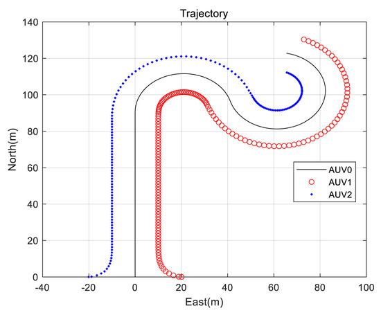
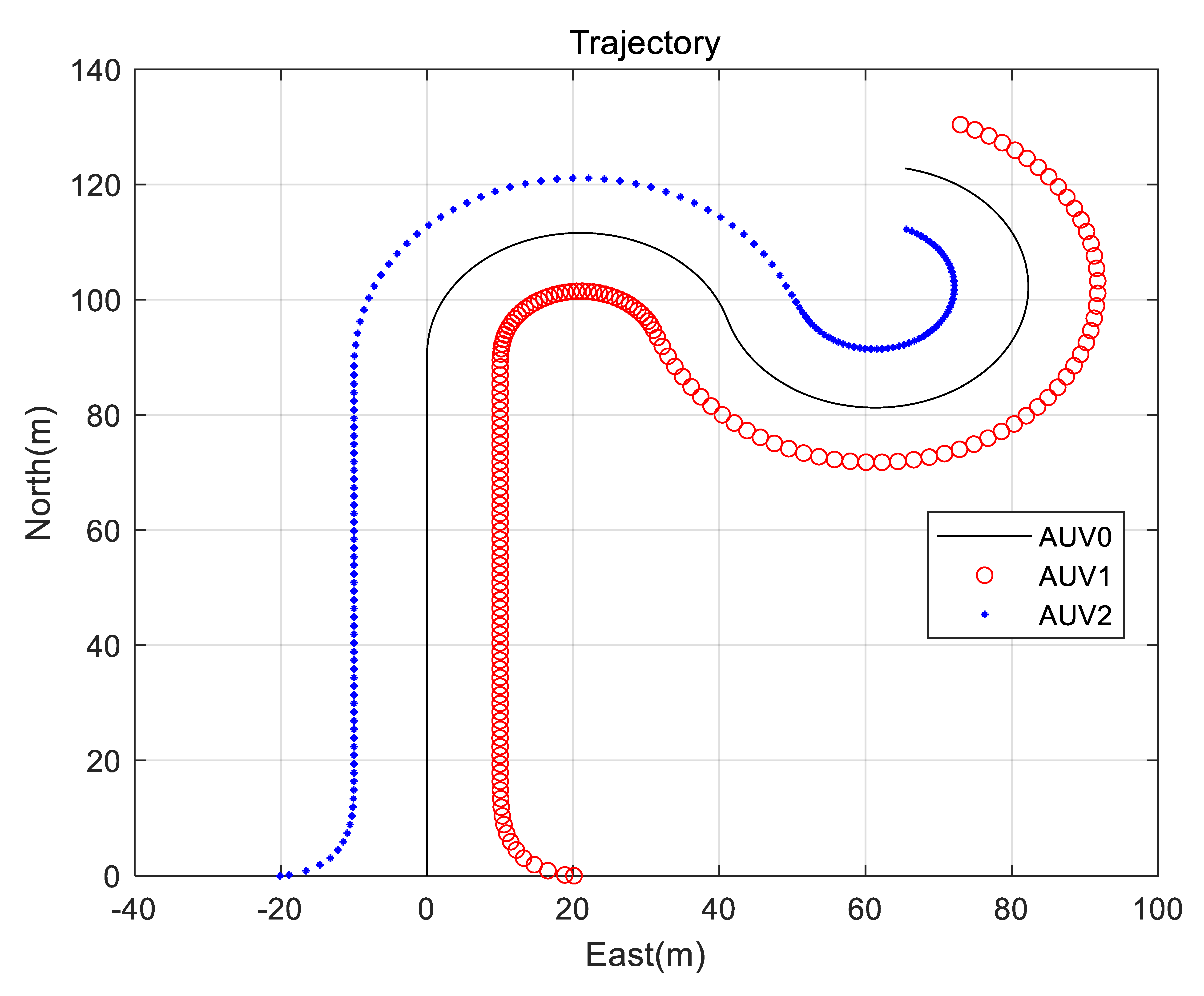
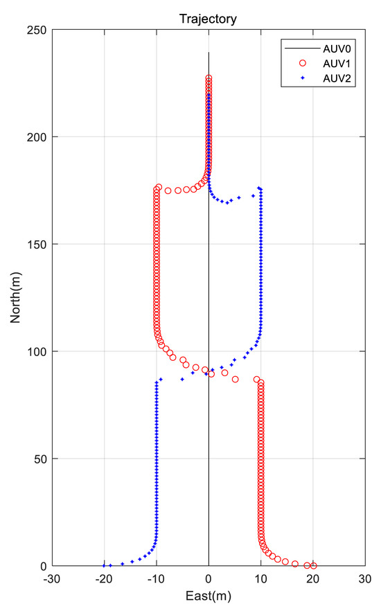
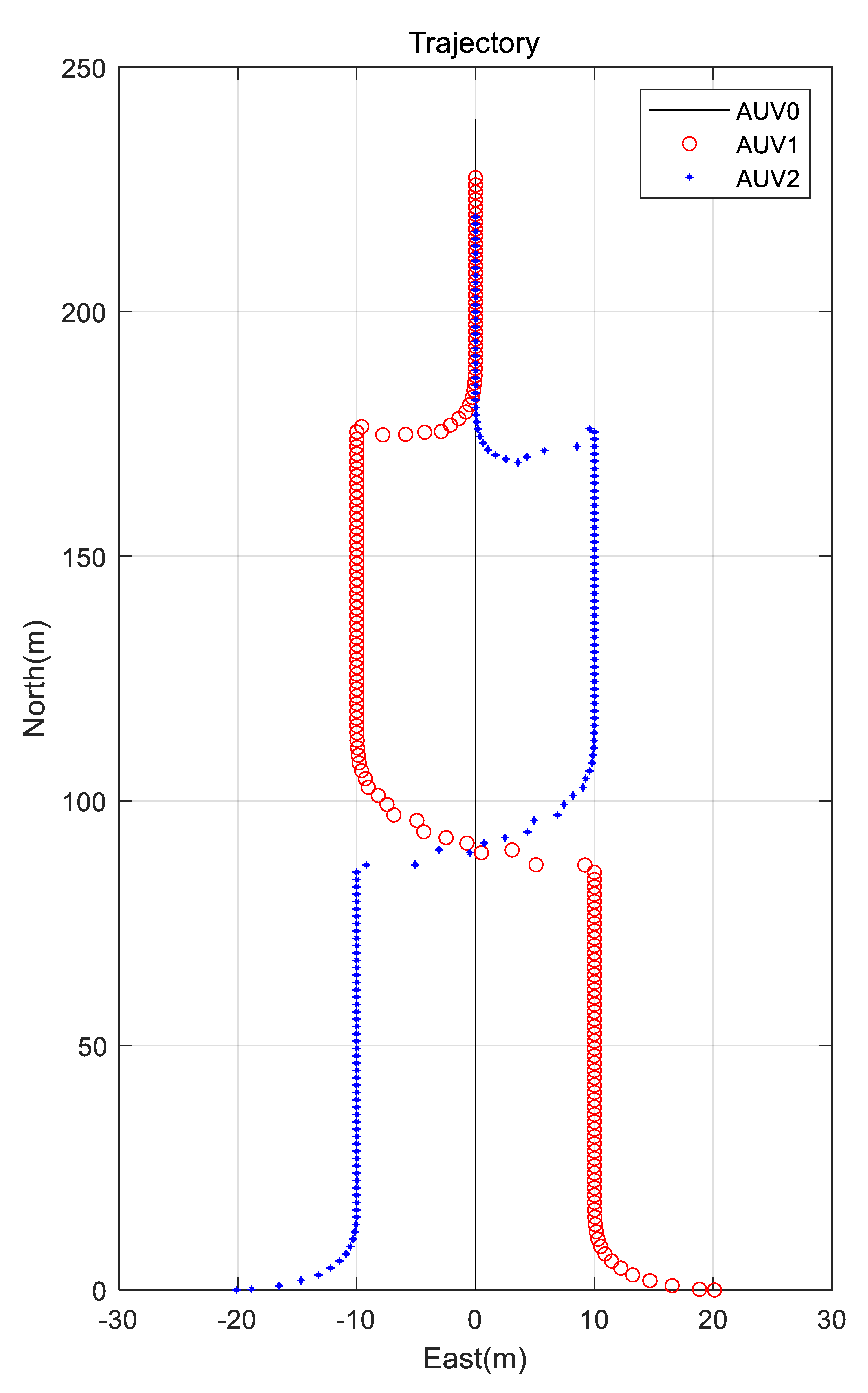
The specific results are as follows (Figure 4):

Figure 4. The trajectories of the AUVs (Case 1).

AUV1 and AUV2 are initially positioned 20 m east and west of AUV0, respectively, with a preset tracking distance of 10 m on both sides. As shown in the results, AUV1 and AUV2 have successfully established a 10-m tracking formation with AUV0 within a very short time. During AUV0’s turning maneuvers, both AUV1 and AUV2 maintain effective distance tracking, demonstrating the effectiveness of the designed tracking control method.

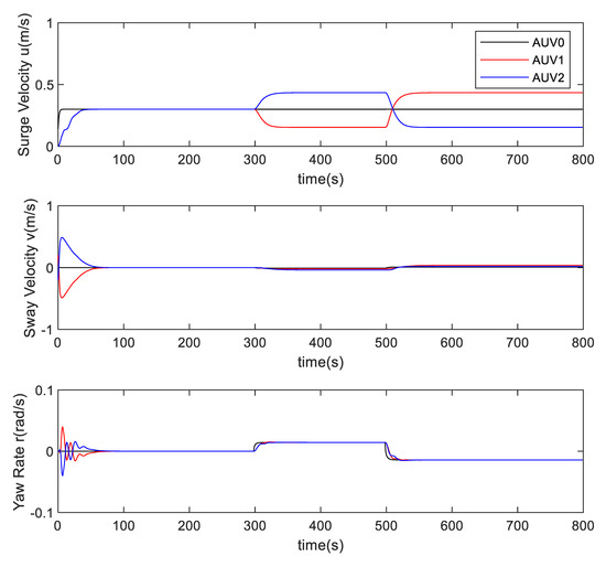
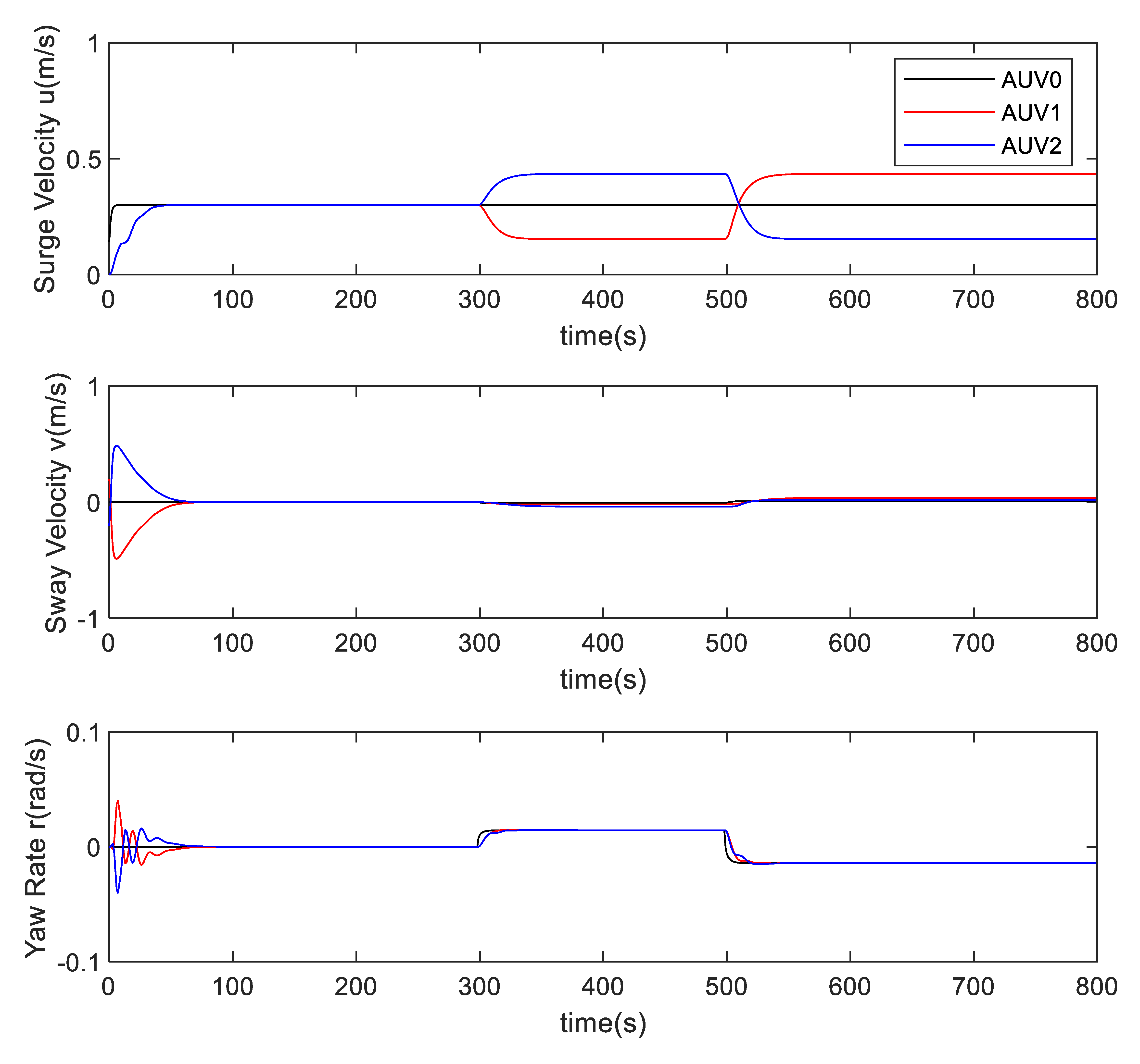
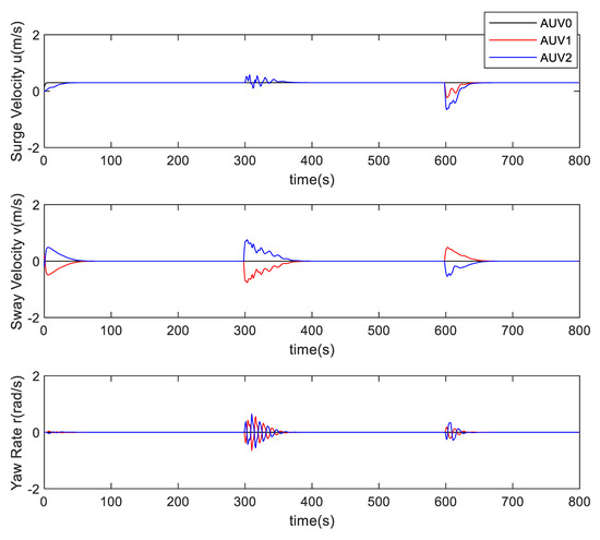
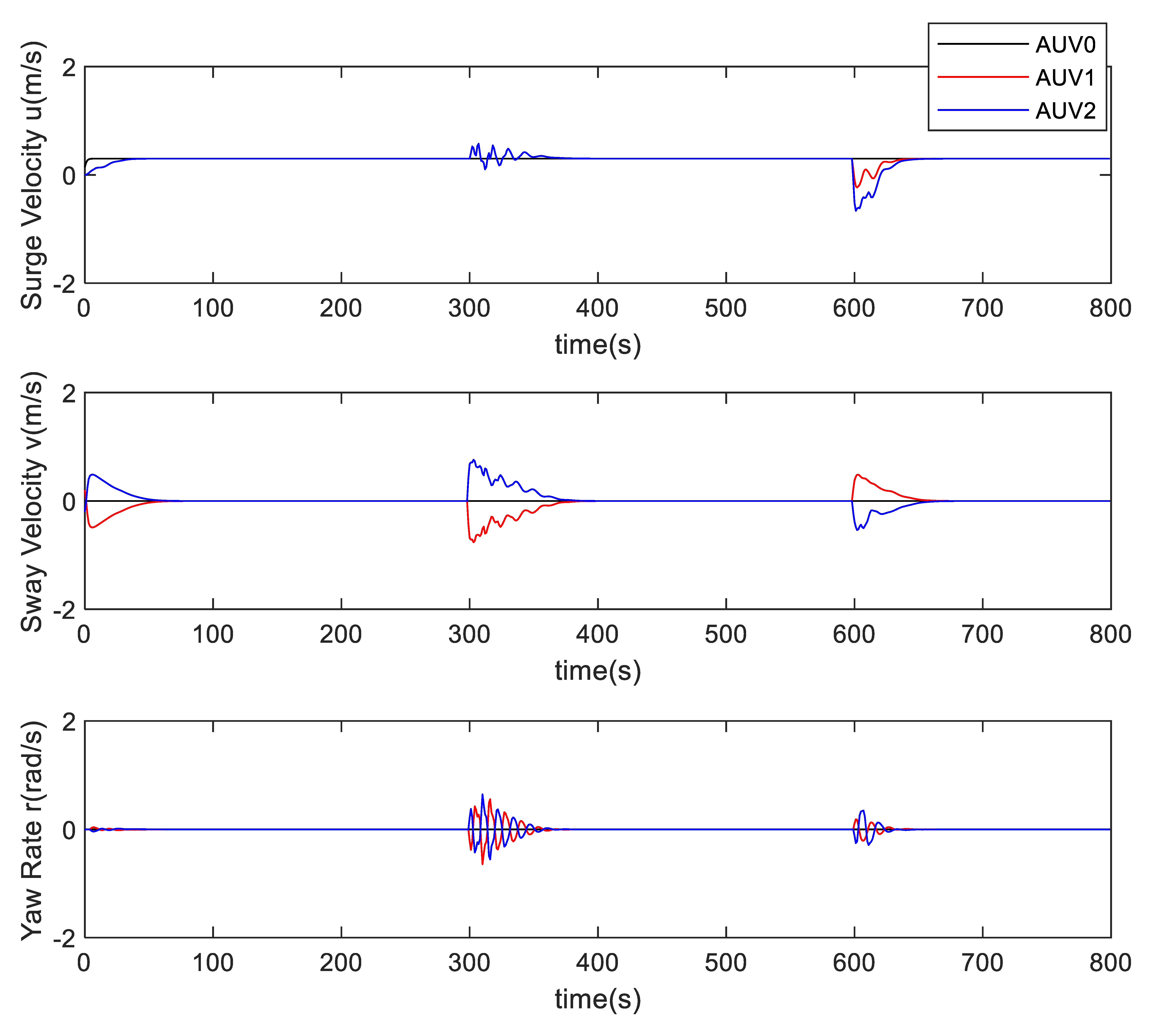
As can be seen from the Figure 5, AUV1 and AUV2 reached the surge velocity of AUV0 at around 30 s, both at approximately 0.25 m/s. At the 300 s mark, they began to follow AUV0 in turning. After the turn, AUV1 decelerated and subsequently stabilized to maintain its relative position with AUV0, while AUV2 accelerated and stabilized to maintain its relative position with AUV0. After 500 s, AUV0 started turning in the opposite direction, at which point AUV1 and AUV2 began to accelerate and decelerate, respectively, to maintain their relative positions with AUV0. From the sway velocity curve, it can be observed that initially, AUV1 and AUV2 generated relatively high speeds to quickly reach their positions 10 m on either side of AUV0. At the 300 s and 500 s marks, AUV1 and AUV2 followed AUV0 in turning, maintaining the same sway velocity as AUV0. In terms of yaw rate, AUV1 and AUV2 initially generated relatively high yaw rates to quickly reach their positions 10 m on either side of AUV0, and their subsequent trends maintained consistency with AUV0.

Figure 5. The speeds and angle speeds of the AUVs (Case 1).

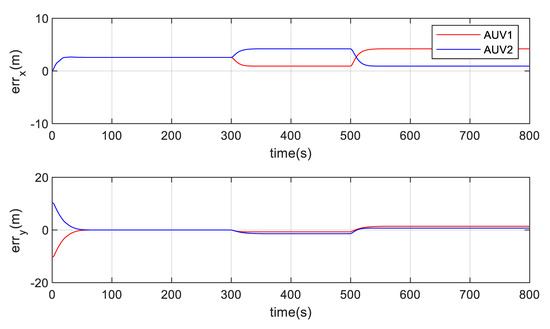
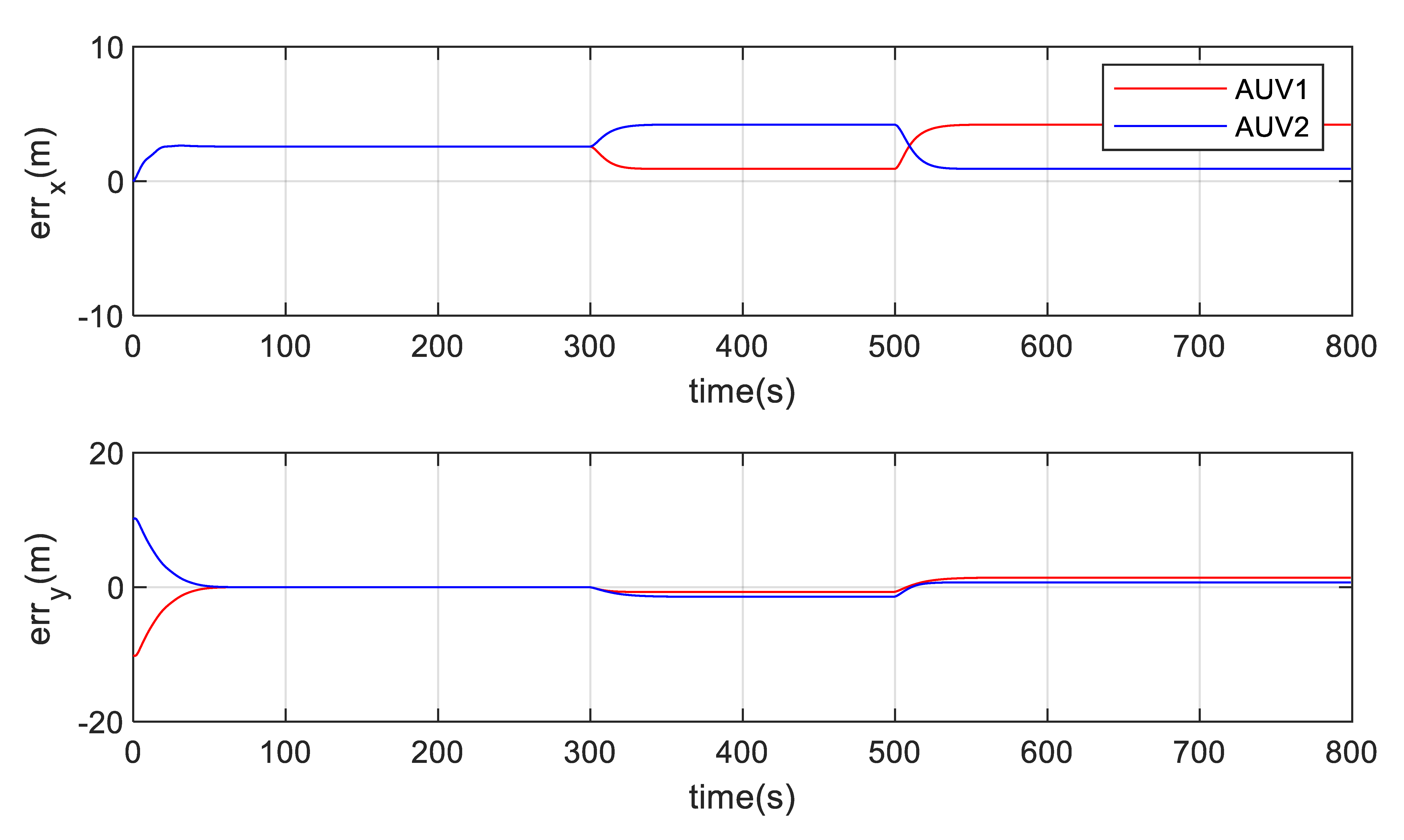
The position deviation curves in Figure 6 represent the surge and sway position deviations of AUV1 and AUV2 from their respective desired tracking target points near AUV0. Err_x is the surge error between desired tracking target points near AUV0 and AUV1/AUV2 in the motion coordinate system of AUV0; Err_y is the sway error between desired tracking target points near AUV0 and AUV1/AUV2 in the motion coordinate system of AUV0. In this simulation, the Np is 40 and Nc is 2; if Np is increased, the tracking trajectory becomes smoother, but the tracking response slows down and the steady-state tracking error increases; if Np is decreased, the tracking response speeds up and the steady-state tracking error decreases, but the path smoothness deteriorates; if Nc is increased, the tracking response accelerates and the tracking error reduces, yet the control input is prone to oscillation during formation switching. Therefore, reasonable parameter configuration is the key to solving the steady-state tracking error. Regarding the surge position deviation, a steady-state error of approximately 2 m exists. This error is attributed to the configuration of the control horizon and prediction horizon and can be further optimized. After 300 s, the error for AUV1 decreases while that for AUV2 increases; after 500 s, the error for AUV1 increases while that for AUV2 decreases. Analysis indicates that these error variations are related to the positions of the two AUVs on the inner and outer tracks during AUV0’s turning maneuvers. The sway error is 10 m at the initial moment, which corresponds to the deviation between AUV1 and its desired tracking target point relative to AUV0. This desired tracking point is located 10 m to either side of AUV0’s position.

Figure 6. The position errors between the AUVs and the target points in the motion coordinate system (Case 1).

5.2. Simulation of Tracking Control for Straight Line Navigation of AUV0 and Transformation of AUV Formation

Set AUV0 to sail in a straight north direction under the influence of control variables, and two slave AUVs to track and control its navigation. AUV1 and AUV2 are initially positioned 20 m east and west of AUV0, respectively. During the tracking process, the formation changes:

Case 2:

Phase 1: the slave AUVs navigate on both sides of the AUV0; the sway distance is 10 m, 0 ≤ t < 300 s;

Phase 2: the two AUVs exchange positions to continue tracking and sailing, 300 ≤ t < 600 s;

Phase 3: the two slave AUVs track and navigate directly behind the AUV0; the surge distances are 8 m and 16 m for AUV1 and AUV2, 600 ≤ t < 800 s.

AUV0 control input is

$${\mathit{\tau }}_0={\left[\begin{array}{cccccc}30& 0& 0& 0& 0& 0\end{array}\right]}^{\mathrm{T}}, t\in [0,800]$$

Through model (1), the state of AUV0 ${\mathit{\eta }}_{AUV0}$ can be obtained. The formation transformation is

$$\left\{\begin{array}{l}\left\{\begin{array}{c}{\mathit{\eta }}_{d_{AUV1}}=\mathit{J}\left({\mathit{J}}^{-1}{\mathit{\eta }}_{AUV0}+\left(0,10,0,0,0,0\right)\right)\\ {\mathit{\eta }}_{d_{AUV2}}=\mathit{J}\left({\mathit{J}}^{-1}{\mathit{\eta }}_{AUV0}+\left(0,-10,0,0,0,0\right)\right)\end{array}\right.\hspace{1em}t\in \left[0,300\right)\hfill \\ \left\{\begin{array}{c}{\mathit{\eta }}_{d_{AUV1}}=\mathit{J}\left({\mathit{J}}^{-1}{\mathit{\eta }}_{AUV0}+\left(0,-10,0,0,0,0\right)\right)\\ {\mathit{\eta }}_{d_{AUV2}}=\mathit{J}\left({\mathit{J}}^{-1}{\mathit{\eta }}_{AUV0}+\left(0,10,0,0,0,0\right)\right)\end{array}\right.\hspace{1em}t\in \left[300,600\right)\hfill \\ \left\{\begin{array}{c}{\mathit{\eta }}_{d_{AUV1}}=\mathit{J}\left({\mathit{J}}^{-1}{\mathit{\eta }}_{AUV0}+\left(-8,0,0,0,0,0\right)\right)\\ {\mathit{\eta }}_{d_{AUV2}}=\mathit{J}\left({\mathit{J}}^{-1}{\mathit{\eta }}_{AUV0}+\left(-16,0,0,0,0,0\right)\right)\end{array}\right.\hspace{1em}t\in \left[600,800\right]\hfill \end{array}\right.$$

(42)

The specific simulation results are as follows (Figure 7):

Figure 7. The trajectories of the AUVs (Case 2).

As shown in the Figure 8, AUV1 and AUV2 reached AUV0’s surge velocity of approximately 0.25 m/s at around 20 s. The sway velocity increased to about 0.5 m/s at around 10 s and decreased to nearly 0 by approximately 50 s, which corresponds to the process of AUV1 and AUV2 maneuvering from their initial positions to the tracking positions on either side of AUV0. At the 300 s mark, AUV1 and AUV2 began to exchange positions. During this maneuver, their surge velocities experienced slight fluctuations but quickly stabilized, while their sway velocities rapidly increased to about 0.8 m/s before decreasing to nearly 0 by around 390 s. Corresponding fluctuations were also observed in their yaw rates. These velocity changes align with the positional exchange maneuver between AUV1 and AUV2. After 600 s, AUV1 and AUV2 tracked AUV0 in a straight line, positioned 8 m and 16 m behind AUV0, respectively. At this stage, AUV2’s speed decreased more significantly than AUV1’s, which is attributed to the difference in their tracking positions along the surge direction. By approximately 630 s, the surge velocities of both AUVs decreased noticeably and stabilized at AUV0’s velocity, indicating that they had reached their respective positions and continued to maintain stable tracking.

Figure 8. The speeds and angle speeds of the AUVs (Case 2).

The position deviation curves in Figure 9 represent the surge and sway position deviations between AUV1/AUV2 and their expected tracking target points near AUV0. Err_x is the surge error between desired tracking target points near AUV0 and AUV1/AUV2 in the motion coordinate system of AUV0; Err_y is the sway error between desired tracking target points near AUV0 and AUV1/AUV2 in the motion coordinate system of AUV0. In this simulation, the Np is 40 and Nc is 2; if Np is increased, the tracking trajectory becomes smoother, but the tracking response slows down and the steady-state tracking error increases; if Np is decreased, the tracking response speeds up and the steady-state tracking error decreases, but the path smoothness deteriorates; if Nc is increased, the tracking response accelerates and the tracking error reduces, yet the control input is prone to oscillation during formation switching. Therefore, reasonable parameter configuration is the key to solving the steady-state tracking error. In terms of surge position deviation, a steady-state error of approximately 1.8 m is observed, which is related to the settings of the control horizon and prediction horizon. The initial sway error measures 10 m. At the 300 s mark, slight fluctuations occur in the surge error, while the sway error expands to 20 m before rapidly decreasing to zero, indicating that AUV1 and AUV2 are exchanging positions. After 600 s, when AUV1 and AUV2 move to different positions directly behind AUV0 and begin straight-line tracking, the sway error rapidly decreases from 10 m to zero, demonstrating that the controller achieves effective tracking control.

Figure 9. The position errors between the AUVs and the target points in the motion coordinate system (Case 2).

5.3. Simulation of Tracking Control and Transformation of AUV Formation with Different Control Methods

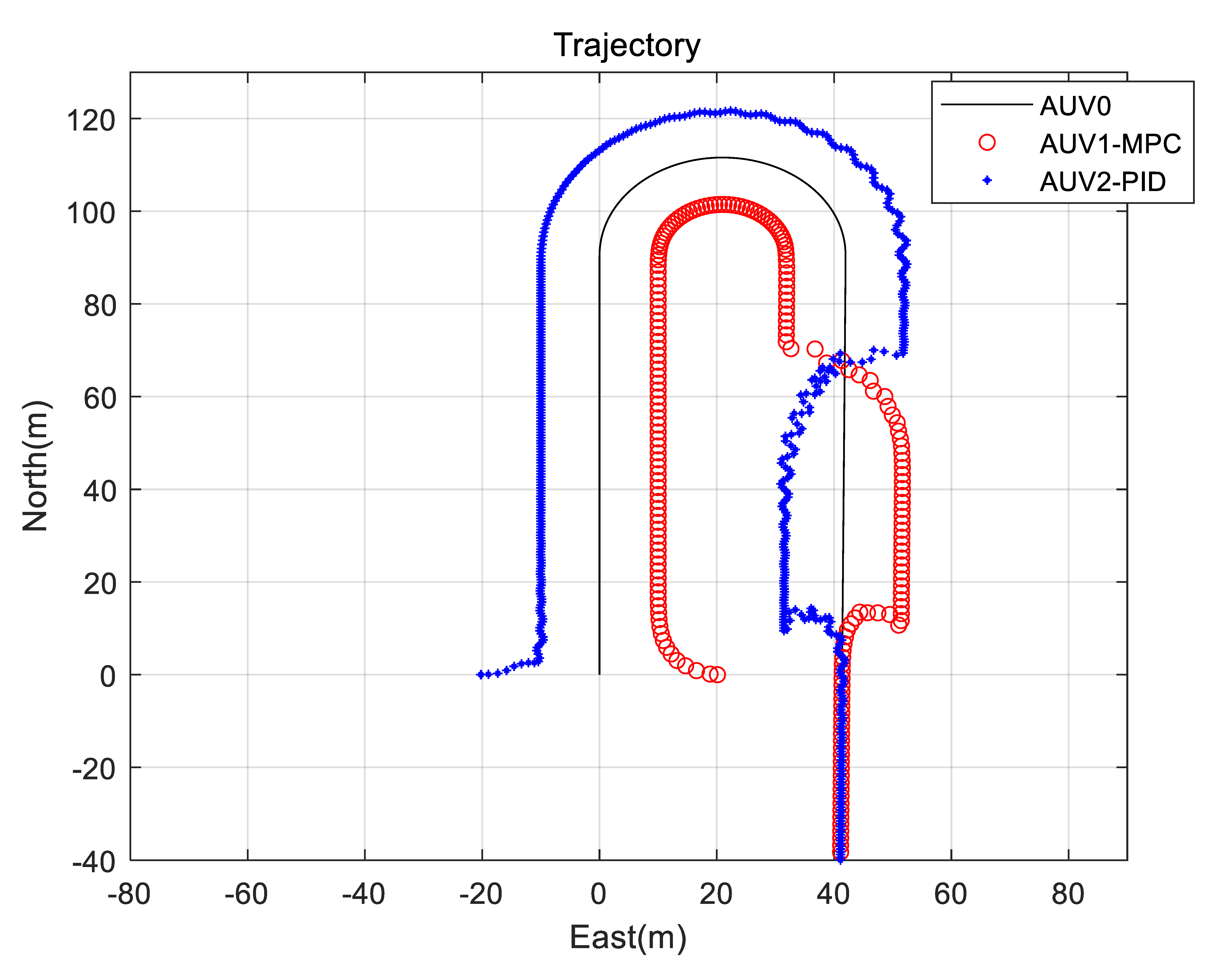
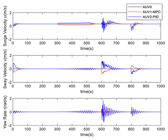
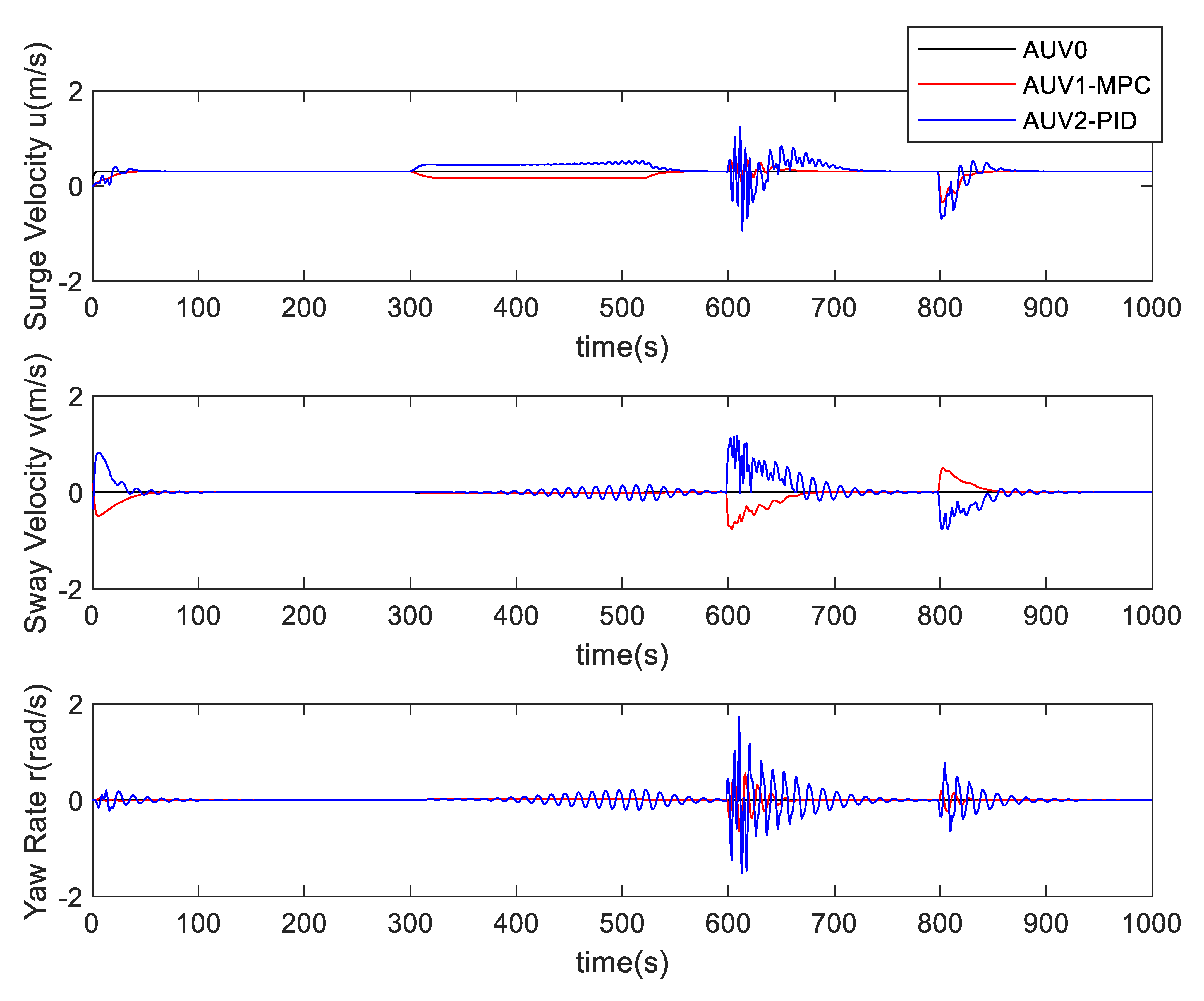
AUV1 and AUV2 start tracking AUV0 from their two respective sides, and swap positions after a period of tracking. AUV1 adopts the MPC method, while AUV2 uses the PID control method. The navigation conditions of the two AUVs are identical except for the initial positions and navigation trajectories. The differences between the two methods are analyzed through symmetric navigation trajectories and state data.

During the tracking process, the formation changes:

Case 3:

Phase 1: the slave AUVs navigate on both sides of the AUV0; the sway distance is 10 m, 0 ≤ t < 600 s;

Phase 2: the two AUVs exchange positions to continue tracking and sailing, 600 ≤ t < 800 s;

Phase 3: two slave AUVs track and navigate directly behind the AUV0; the surge distance is 10 m for AUV1 and AUV2, 800 ≤ t < 1000 s.

AUV0 control input is

$${\mathit{\tau }}_0=\left\{\begin{array}{l}{\left[\begin{array}{cccccc}30& 0& 0& 0& 0& 0\end{array}\right]}^{\mathrm{T}},\hspace{1em}t\in [0,300)\hfill \\ {\left[\begin{array}{cccccc}30& 0& 0& 0& 0& 0.6\end{array}\right]}^{\mathrm{T}},\hspace{1em}t\in [300,520)\hfill \\ {\left[\begin{array}{cccccc}30& 0& 0& 0& 0& 0\end{array}\right]}^{\mathrm{T}},\hspace{1em}t\in [520,1000]\hfill \end{array}\right.$$

Through model (1), the state of AUV0 ${\mathit{\eta }}_{AUV0}$ can be obtained. The formation transformation is

$$\left\{\begin{array}{l}\left\{\begin{array}{c}{\mathit{\eta }}_{d_{AUV1}}=\mathit{J}\left({\mathit{J}}^{-1}{\mathit{\eta }}_{AUV0}+\left(0,10,0,0,0,0\right)\right)\\ {\mathit{\eta }}_{d_{AUV2}}=\mathit{J}\left({\mathit{J}}^{-1}{\mathit{\eta }}_{AUV0}+\left(0,-10,0,0,0,0\right)\right)\end{array}\right.\hspace{1em}t\in \left[0,600\right)\hfill \\ \left\{\begin{array}{c}{\mathit{\eta }}_{d_{AUV1}}=\mathit{J}\left({\mathit{J}}^{-1}{\mathit{\eta }}_{AUV0}+\left(0,-10,0,0,0,0\right)\right)\\ {\mathit{\eta }}_{d_{AUV2}}=\mathit{J}\left({\mathit{J}}^{-1}{\mathit{\eta }}_{AUV0}+\left(0,10,0,0,0,0\right)\right)\end{array}\right.\hspace{1em}t\in \left[600,800\right)\hfill \\ \left\{\begin{array}{c}{\mathit{\eta }}_{d_{AUV1}}=\mathit{J}\left({\mathit{J}}^{-1}{\mathit{\eta }}_{AUV0}+\left(-10,0,0,0,0,0\right)\right)\\ {\mathit{\eta }}_{d_{AUV2}}=\mathit{J}\left({\mathit{J}}^{-1}{\mathit{\eta }}_{AUV0}+\left(-10,0,0,0,0,0\right)\right)\end{array}\right.\hspace{1em}t\in \left[800,1000\right]\hfill \end{array}\right.$$

The specific simulation results are as follows (Figure 10):

Figure 10. The trajectories of the AUVs (Case 3).

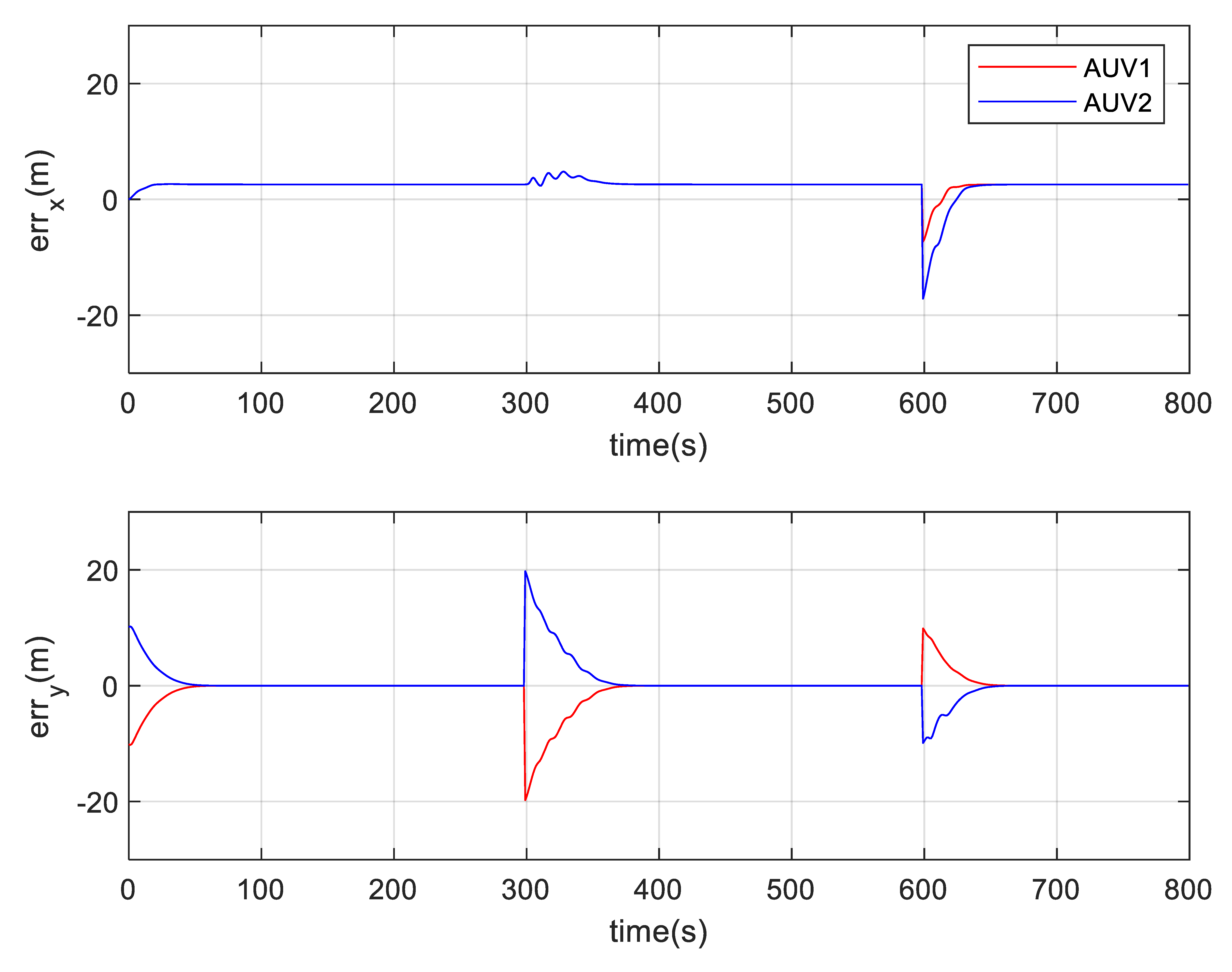
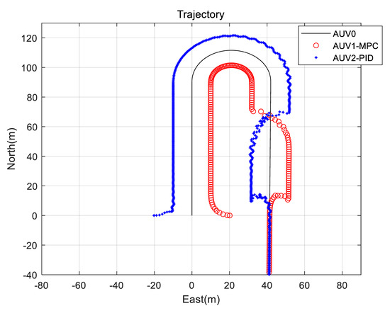
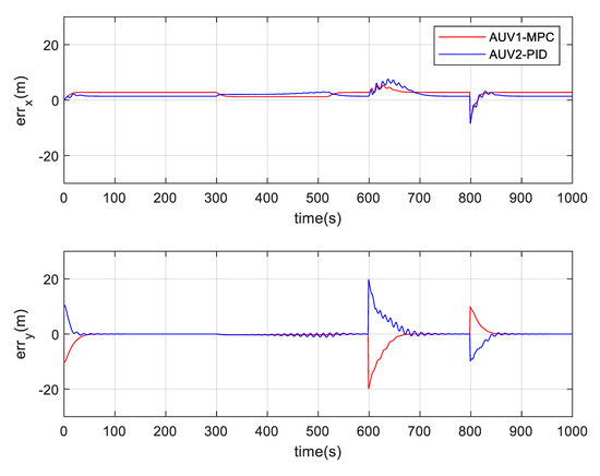
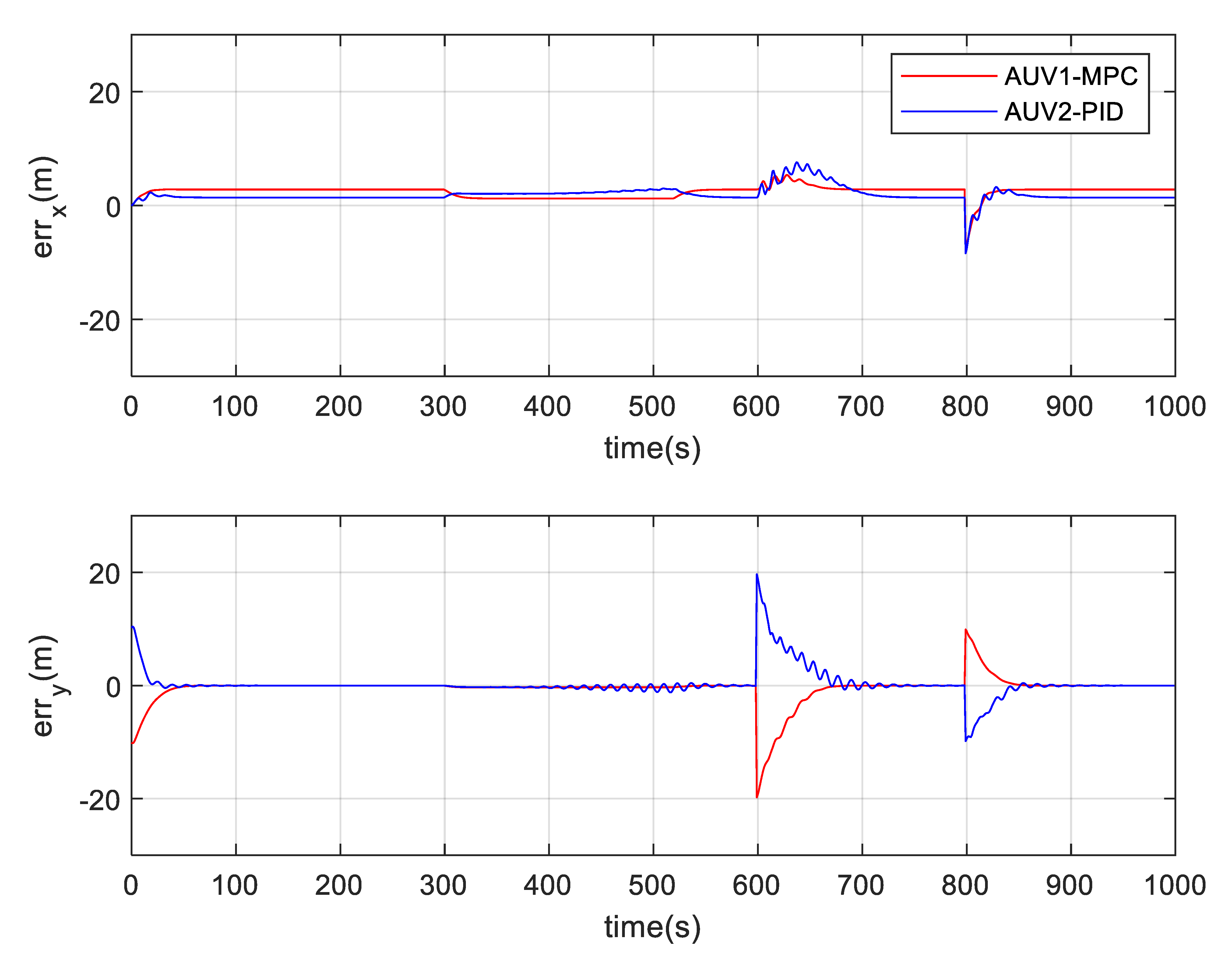
As shown in Figure 11, AUV1 and AUV2 reached AUV0’s surge velocity of approximately 0.25 m/s at around 20 s. The sway velocity increased to about 0.5 m/s at around 10 s and decreased to nearly 0 by approximately 50 s, which corresponds to the process of AUV1 and AUV2 maneuvering from their initial positions to the tracking positions on either side of AUV0. The variation amplitude and fluctuation of the PID method are significantly worse than those of the MPC method. At 600 s, significant positional changes occurred in the slave AUVs, as they shifted from one side to the other of the master AUV. According to the data results, during this process, the maximum surge transient error under MPC control was 4.7 m, and the maximum sway transient error was 20 m. In contrast, under PID control, the maximum surge transient error was 8.2 m, and the maximum sway transient error was 20 m. This demonstrates that the MPC method effectively reduces the surge transient error, resulting in more stable tracking performance of the slave AUVs. Due to the sudden jump of the target formation to be tracked, the robustness of the PID method is slightly slower than that of the MPC method when multiple variables jump simultaneously and various constraints need to be handled at the same time.

Figure 11. The speeds and angle speeds of the AUVs (Case 3).

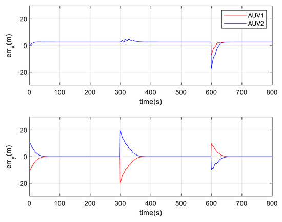
The position deviation curves in Figure 12 represent the surge and sway position deviations between AUV1/AUV2 and their expected tracking target points near AUV0. Err_x is the surge error between desired tracking target points near AUV0 and AUV1/AUV2 in the motion coordinate system of AUV0; Err_y is the sway error between desired tracking target points near AUV0 and AUV1/AUV2 in the motion coordinate system of AUV0. In terms of the steady-state errors in surge and sway directions, the surge steady-state error of the PID method during the straight-line tracking phase is 0.9 m, which is significantly smaller than the 1.8 m surge steady-state error of the MPC method; However, during the curve turning tracking phase and the formation transformation phase, the surge and the sway errors of the PID method are significantly larger than those of the MPC method. This indicates that in the tracking control of multi-input–multi-output systems, the MPC method has better robustness in handing multiple constraints simultaneously, while the PID method achieves smaller steady-state errors during the straight-line tracking phase.

Figure 12. The position errors between the AUVs and the target points in the motion coordinate system (Case 3).

5.4. Simulation of Tracking Control for Two Subordinate AUVs at Different Depths and Exchange Positions

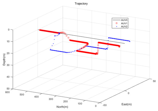
The master AUV travels in a straight line along the due north direction, and the two slave AUVs track the master while performing formation transformations. The experiment is divided into four phases:

Case 4:

Phase 1: The two slave AUVs track the master while maintaining a sway offset of 10 m on either side, 0 ≤ t < 500 s.

Phase 2: Building on Phase 1, the two slave AUVs descend 10 m while continuing to track the master, 500 ≤ t < 1000 s.

Phase 3: Based on Phase 2, the two slave AUVs swap left and right positions and expand the distance to 20 m from the master, 1000 ≤ t < 1500 s.

Phase 4: Following Phase 3, the two slave AUVs ascend and transition to tracking the master in a straight line directly behind it, 1500 ≤ t < 2000 s.

AUV0 control input is

$${\mathit{\tau }}_0={\left[\begin{array}{cccccc}30& 0& 0& 0& 0& 0\end{array}\right]}^{\mathrm{T}},\hspace{1em}t\in [0,800]$$

Through model (1), the state of AUV0 ${\mathit{\eta }}_{AUV0}$ can be obtained. The formation transformation is

$$\left\{\begin{array}{l}\left\{\begin{array}{c}{\mathit{\eta }}_{d_{AUV1}}=\mathit{J}\left({\mathit{J}}^{-1}{\mathit{\eta }}_{AUV0}+\left(0,-10,0,0,0,0\right)\right)\\ {\mathit{\eta }}_{d_{AUV2}}=\mathit{J}\left({\mathit{J}}^{-1}{\mathit{\eta }}_{AUV0}+\left(0,10,0,0,0,0\right)\right)\end{array}\right.\hspace{1em}t\in \left[0,500\right)\hfill \\ \left\{\begin{array}{c}{\mathit{\eta }}_{d_{AUV1}}=\mathit{J}\left({\mathit{J}}^{-1}{\mathit{\eta }}_{AUV0}+\left(0,-10,10,0,0,0\right)\right)\\ {\mathit{\eta }}_{d_{AUV2}}=\mathit{J}\left({\mathit{J}}^{-1}{\mathit{\eta }}_{AUV0}+\left(0,10,10,0,0,0\right)\right)\end{array}\right.\hspace{1em}t\in \left[500,1000\right)\hfill \\ \left\{\begin{array}{c}{\mathit{\eta }}_{d_{AUV1}}=\mathit{J}\left({\mathit{J}}^{-1}{\mathit{\eta }}_{AUV0}+\left(0,20,10,0,0,0\right)\right)\\ {\mathit{\eta }}_{d_{AUV2}}=\mathit{J}\left({\mathit{J}}^{-1}{\mathit{\eta }}_{AUV0}+\left(0,-20,10,0,0,0\right)\right)\end{array}\right.\hspace{1em}t\in \left[1000,1500\right)\hfill \\ \left\{\begin{array}{c}{\mathit{\eta }}_{d_{AUV1}}=\mathit{J}\left({\mathit{J}}^{-1}{\mathit{\eta }}_{AUV0}+\left(-10,0,0,0,0,0\right)\right)\\ {\mathit{\eta }}_{d_{AUV2}}=\mathit{J}\left({\mathit{J}}^{-1}{\mathit{\eta }}_{AUV0}+\left(-20,0,0,0,0,0\right)\right)\end{array}\right.\hspace{1em}t\in \left[1500,2000\right]\hfill \end{array}\right.$$

The specific simulation results are as follows (Figure 13, Figure 14 and Figure 15):

Figure 13. The trajectories of the AUVs (Case 4).

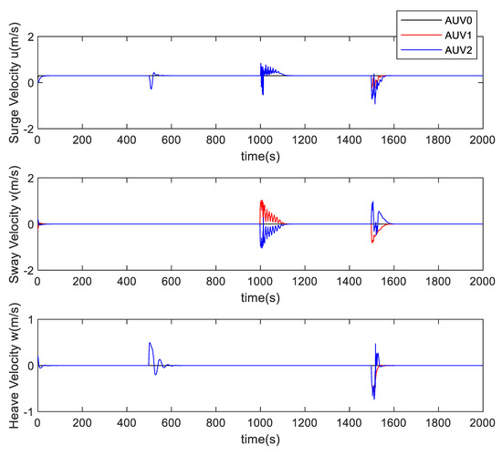
Figure 14. The speeds and angle speeds of the AUVs (Case 4).

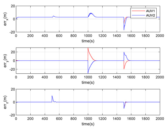
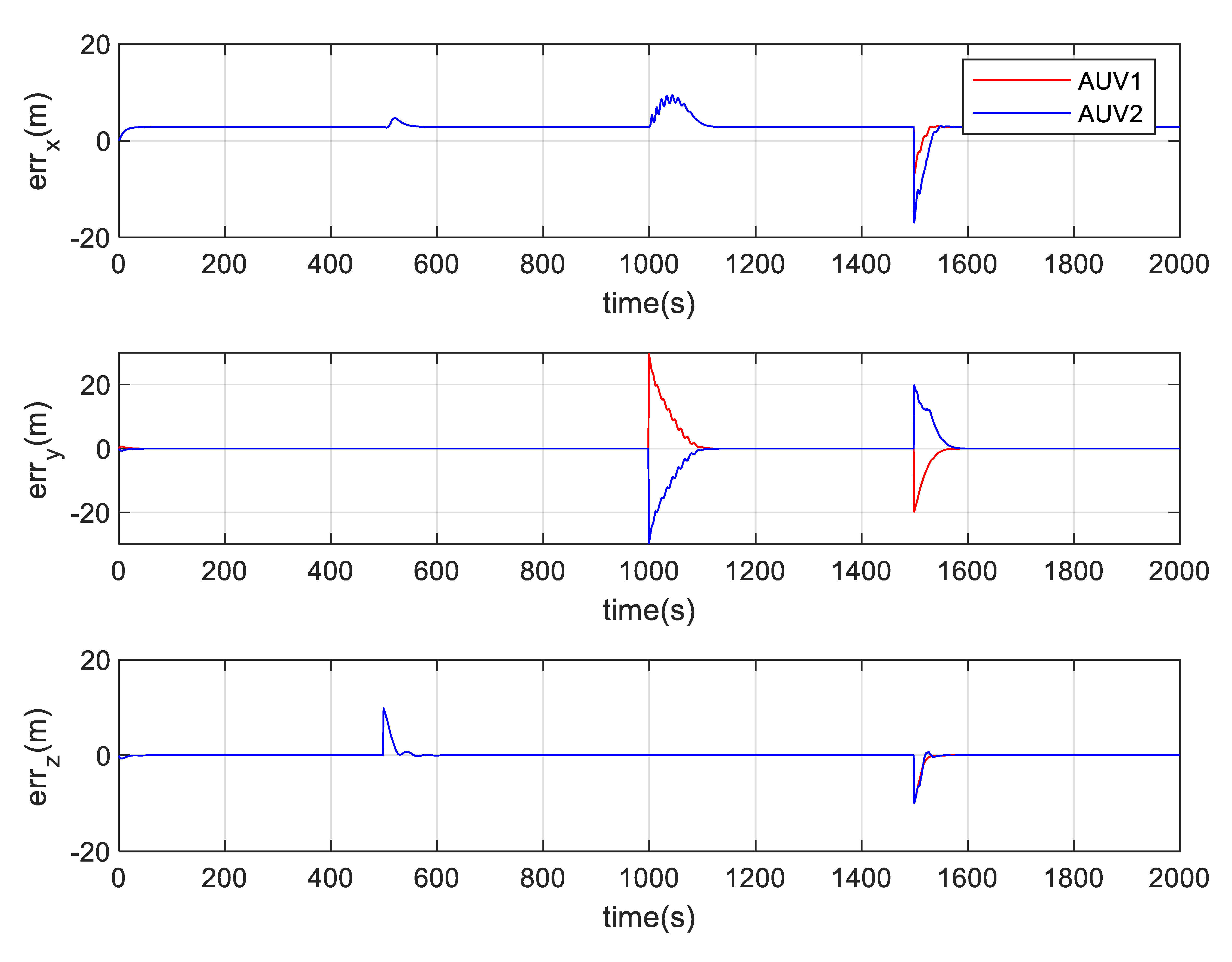
Figure 15. The position errors between the AUVs and the target points in the motion coordinate system (Case 4).

From the perspective of surge velocity, a slight fluctuation occurred at 500 s, which quickly stabilized to 0.4 m/s within 20 s. The sway velocity remained unchanged, while the heave velocity shifted from 0 to 0.5 m/s and then stabilized at 0 by the 600 s mark. This behavior corresponds to the process where the AUVs, after tracking in a straight line on both sides, initiated a diving maneuver to continue straight-line tracking without any change in sway target position.

At the 1000 s mark, AUV1 and AUV2 exchanged positions and expanded the sway tracking distance from 10 m to 20 m. During this process, no heave movement occurred, so the heave velocity showed no fluctuation. However, significant fluctuations were observed in both surge and sway velocities, which quickly stabilized.

By the 1500 s mark, AUV1 and AUV2 surfaced and navigated to different positions directly behind AUV0. At this point, the surge velocity fluctuated, while the sway velocities of the two AUVs changed in opposite directions. The heave velocity exhibited a trend opposite to that during the diving maneuver, reaching a maximum of approximately −0.5 m/s.

Err_x is the surge error between desired tracking target points near AUV0 and AUV1/AUV2 in the motion coordinate system of AUV0; Err_y is the sway error between desired tracking target points near AUV0 and AUV1/AUV2 in the motion coordinate system of AUV0; Err_z is the heave error between desired tracking target points near AUV0 and AUV1/AUV2 in the motion coordinate system of AUV0. As analyzed previously, a steady-state error of 1.5 m exists in the surge direction, while both sway and heave errors remain zero. In this simulation, the Np is 40 and Nc is 2; if Np is increased, the tracking trajectory becomes smoother, but the tracking response slows down and the steady-state tracking error increases; if Np is decreased, the tracking response speeds up and the steady-state tracking error decreases, but the path smoothness deteriorates; If Nc is increased, the tracking response accelerates and the tracking error reduces, yet the control input is prone to oscillation during formation switching. Therefore, reasonable parameter configuration is the key to solving the steady-state tracking error. Throughout the tracking process, when the AUV’s position changes, the error trends in all three directions align with the movement patterns and stabilize rapidly, which demonstrates the effectiveness of the adopted tracking control method.

Throughout the simulation, the two slave AUVs successfully execute the formation transformations while maintaining stable tracking of the master AUV.

5.5. Simulation of Tracking Control for Six Subordinate AUVs at Different Depths and Exchange Positions

The master AUV travels in a straight line along the due north direction, and the six slave AUVs track the master while performing formation transformations. The experiment is divided into four phases:

Case 5:

Phase 1: The six slave AUVs track the master while maintaining a sway offset of different distances on either side, 0 ≤ t < 500 s.

Phase 2: Building on Phase 1, the six slave AUVs change the depth and position while continuing to track the master, 500 ≤ t < 1000 s.

Phase 3: Based on Phase 2, the six slave AUVs change their formation and remain at the same depth as the master, 1000 ≤ t < 1500 s.

Phase 4: Following Phase 3, the six slave AUVs ascend and transition to tracking the master in a straight line directly behind it, 1500 ≤ t < 2000 s.

AUV0 control input is

$${\mathit{\tau }}_0={\left[\begin{array}{cccccc}30& 0& 0& 0& 0& 0\end{array}\right]}^{\mathrm{T}},\hspace{1em}t\in [0,2000]$$

Through model (1), the state of AUV0 ${\mathit{\eta }}_{AUV0}$ can be obtained. The formation transformation is

$$\left\{\begin{array}{l}\left\{\begin{array}{c}{\mathit{\eta }}_{d_{AUV1}}=\mathit{J}\left({\mathit{J}}^{-1}{\mathit{\eta }}_{AUV0}+\left(-5,-5,0,0,0,0\right)\right)\\ {\mathit{\eta }}_{d_{AUV2}}=\mathit{J}\left({\mathit{J}}^{-1}{\mathit{\eta }}_{AUV0}+\left(-10,-10,0,0,0,0\right)\right)\\ {\mathit{\eta }}_{d_{AUV3}}=\mathit{J}\left({\mathit{J}}^{-1}{\mathit{\eta }}_{AUV0}+\left(-15,-15,0,0,0,0\right)\right)\\ {\mathit{\eta }}_{d_{AUV4}}=\mathit{J}\left({\mathit{J}}^{-1}{\mathit{\eta }}_{AUV0}+\left(-5,5,0,0,0,0\right)\right)\\ {\mathit{\eta }}_{d_{AUV5}}=\mathit{J}\left({\mathit{J}}^{-1}{\mathit{\eta }}_{AUV0}+\left(-10,10,0,0,0,0\right)\right)\\ {\mathit{\eta }}_{d_{AUV6}}=\mathit{J}\left({\mathit{J}}^{-1}{\mathit{\eta }}_{AUV0}+\left(-15,15,0,0,0,0\right)\right)\end{array}\right.\hspace{1em}t\in \left[0,500\right)\hfill \\ \left\{\begin{array}{c}{\mathit{\eta }}_{d_{AUV1}}=\mathit{J}\left({\mathit{J}}^{-1}{\mathit{\eta }}_{AUV0}+\left(0,-20,0,0,0,0\right)\right)\\ {\mathit{\eta }}_{d_{AUV2}}=\mathit{J}\left({\mathit{J}}^{-1}{\mathit{\eta }}_{AUV0}+\left(0,-20,-10,0,0,0\right)\right)\\ {\mathit{\eta }}_{d_{AUV3}}=\mathit{J}\left({\mathit{J}}^{-1}{\mathit{\eta }}_{AUV0}+\left(0,-20,10,0,0,0\right)\right)\\ {\mathit{\eta }}_{d_{AUV4}}=\mathit{J}\left({\mathit{J}}^{-1}{\mathit{\eta }}_{AUV0}+\left(0,20,0,0,0,0\right)\right)\\ {\mathit{\eta }}_{d_{AUV5}}=\mathit{J}\left({\mathit{J}}^{-1}{\mathit{\eta }}_{AUV0}+\left(0,20,-10,0,0,0\right)\right)\\ {\mathit{\eta }}_{d_{AUV6}}=\mathit{J}\left({\mathit{J}}^{-1}{\mathit{\eta }}_{AUV0}+\left(0,20,10,0,0,0\right)\right)\end{array}\right.\hspace{1em}t\in \left[500,1000\right)\hfill \\ \left\{\begin{array}{c}{\mathit{\eta }}_{d_{AUV1}}=\mathit{J}\left({\mathit{J}}^{-1}{\mathit{\eta }}_{AUV0}+\left(0,5,0,0,0,0\right)\right)\\ {\mathit{\eta }}_{d_{AUV2}}=\mathit{J}\left({\mathit{J}}^{-1}{\mathit{\eta }}_{AUV0}+\left(0,10,0,0,0,0\right)\right)\\ {\mathit{\eta }}_{d_{AUV3}}=\mathit{J}\left({\mathit{J}}^{-1}{\mathit{\eta }}_{AUV0}+\left(0,15,0,0,0,0\right)\right)\\ {\mathit{\eta }}_{d_{AUV4}}=\mathit{J}\left({\mathit{J}}^{-1}{\mathit{\eta }}_{AUV0}+\left(0,-5,0,0,0,0\right)\right)\\ {\mathit{\eta }}_{d_{AUV5}}=\mathit{J}\left({\mathit{J}}^{-1}{\mathit{\eta }}_{AUV0}+\left(0,-10,0,0,0,0\right)\right)\\ {\mathit{\eta }}_{d_{AUV6}}=\mathit{J}\left({\mathit{J}}^{-1}{\mathit{\eta }}_{AUV0}+\left(0,-15,0,0,0,0\right)\right)\end{array}\right.\hspace{1em}t\in \left[1000,1500\right)\hfill \\ \left\{\begin{array}{c}{\mathit{\eta }}_{d_{AUV1}}=\mathit{J}\left({\mathit{J}}^{-1}{\mathit{\eta }}_{AUV0}+\left(-5,0,0,0,0,0\right)\right)\\ {\mathit{\eta }}_{d_{AUV2}}=\mathit{J}\left({\mathit{J}}^{-1}{\mathit{\eta }}_{AUV0}+\left(-10,0,0,0,0,0\right)\right)\\ {\mathit{\eta }}_{d_{AUV3}}=\mathit{J}\left({\mathit{J}}^{-1}{\mathit{\eta }}_{AUV0}+\left(-15,0,0,0,0,0\right)\right)\\ {\mathit{\eta }}_{d_{AUV4}}=\mathit{J}\left({\mathit{J}}^{-1}{\mathit{\eta }}_{AUV0}+\left(-20,0,0,0,0,0\right)\right)\\ {\mathit{\eta }}_{d_{AUV5}}=\mathit{J}\left({\mathit{J}}^{-1}{\mathit{\eta }}_{AUV0}+\left(-25,0,0,0,0,0\right)\right)\\ {\mathit{\eta }}_{d_{AUV6}}=\mathit{J}\left({\mathit{J}}^{-1}{\mathit{\eta }}_{AUV0}+\left(-30,0,0,0,0,0\right)\right)\end{array}\right.\hspace{1em}t\in \left[1500,2000\right]\hfill \end{array}\right.$$

The specific simulation results are as follows (Figure 16, Figure 17, Figure 18, Figure 19 and Figure 20):

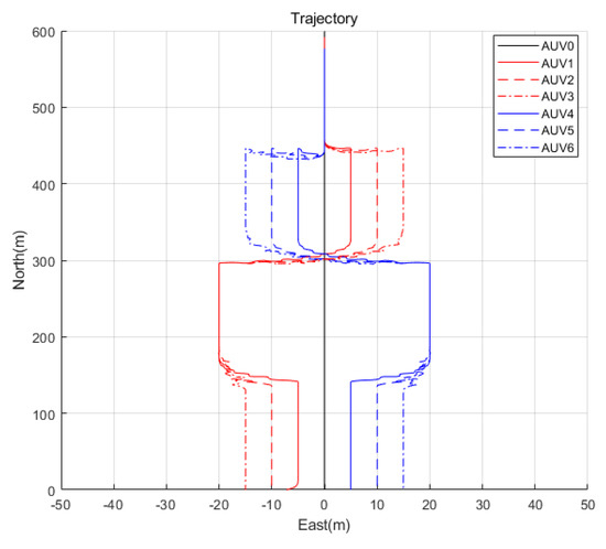
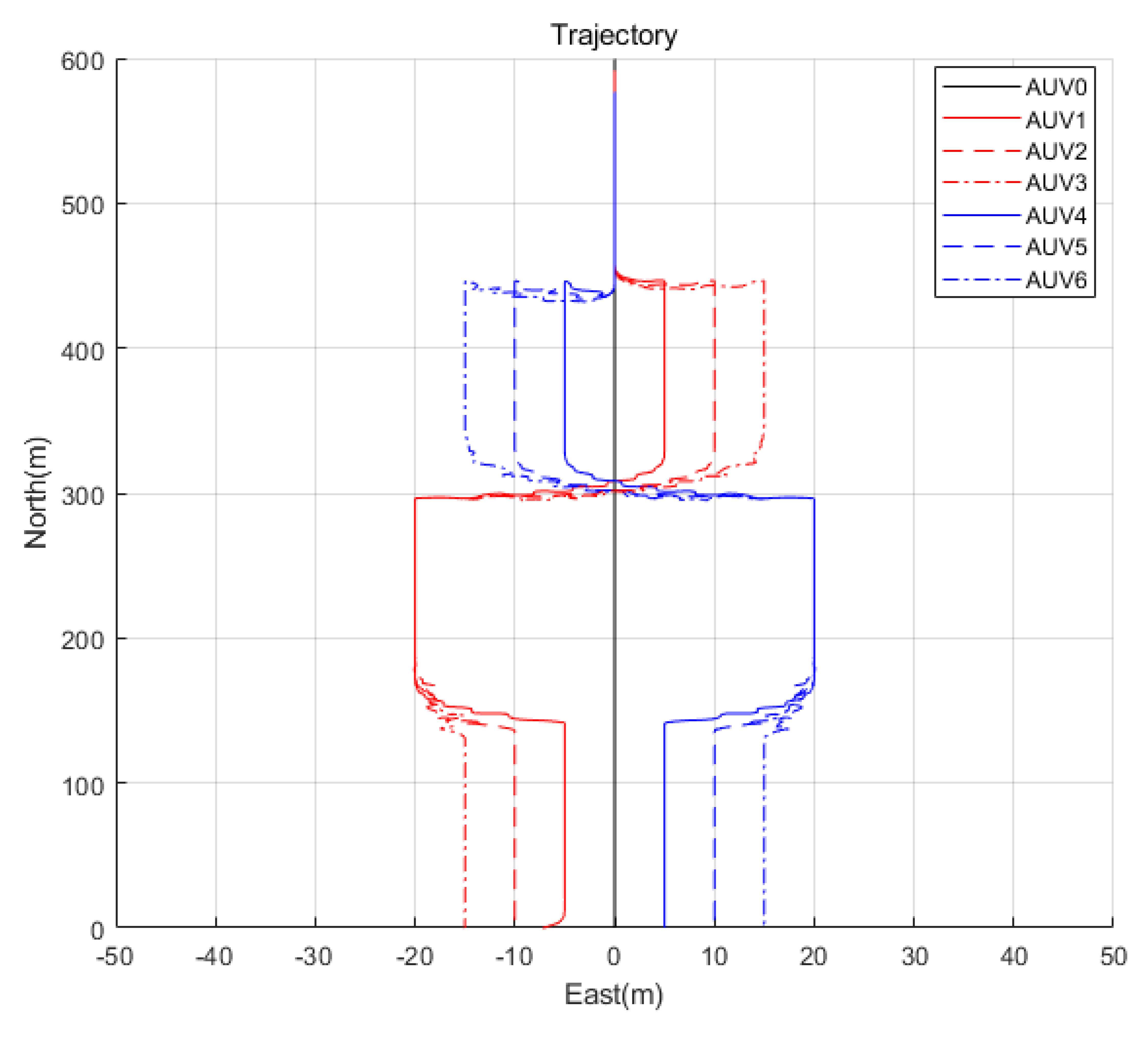
Figure 16. The trajectories of the AUVs in the east and north directions (Case 5).

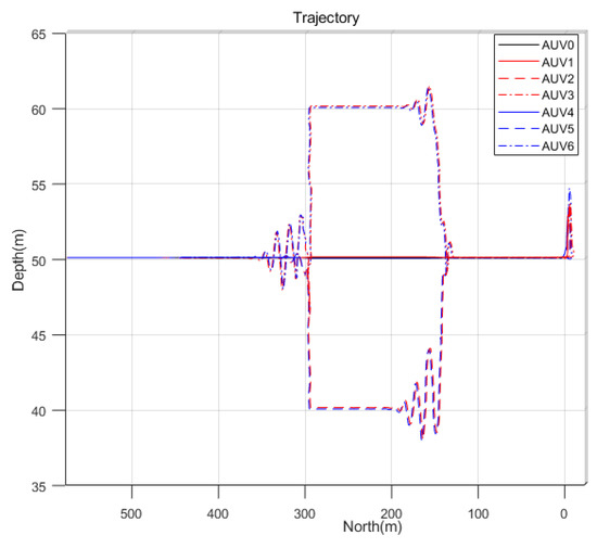
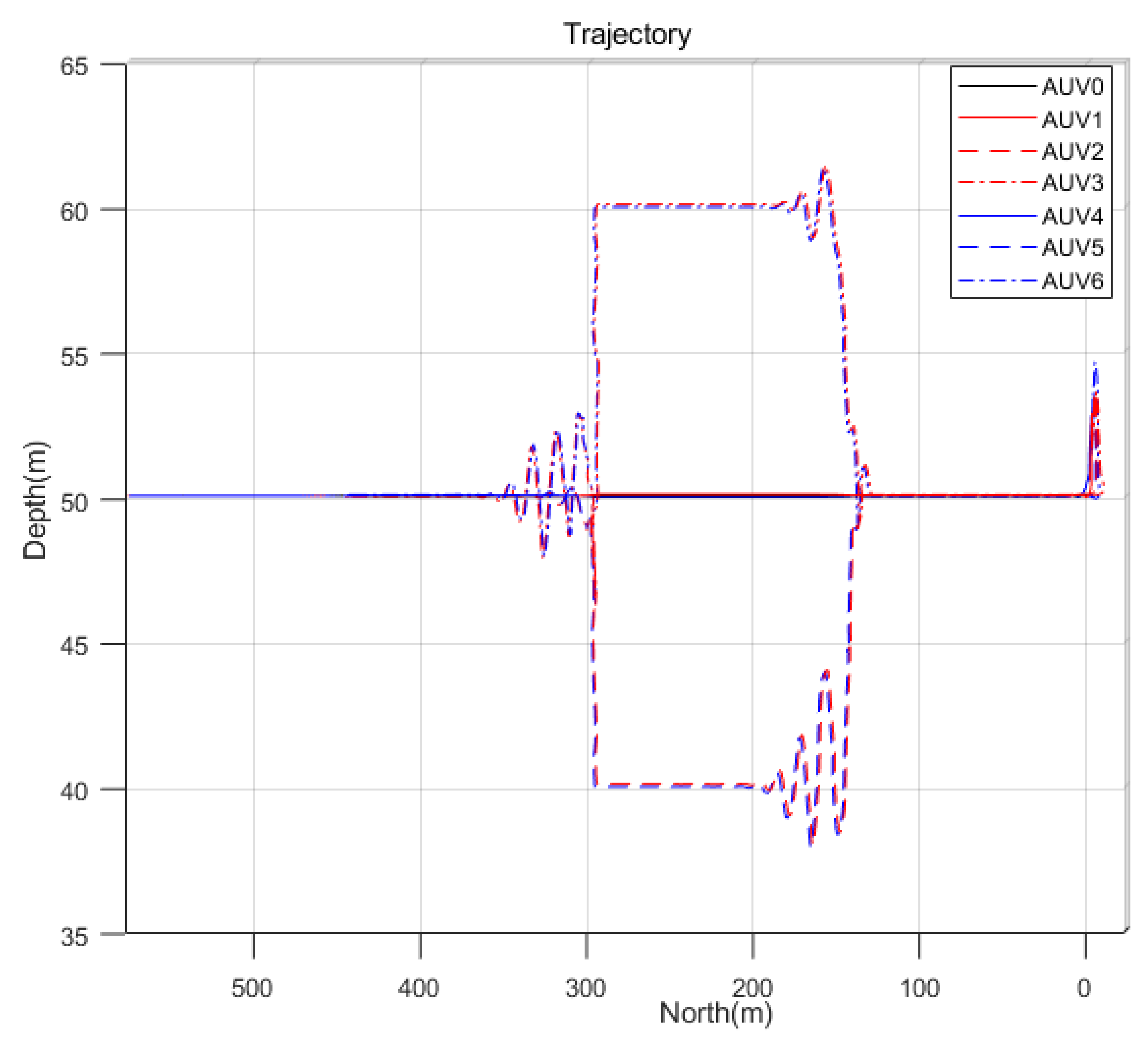
Figure 17. The trajectories of the AUVs in the north and depth directions (Case 5).

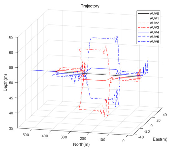
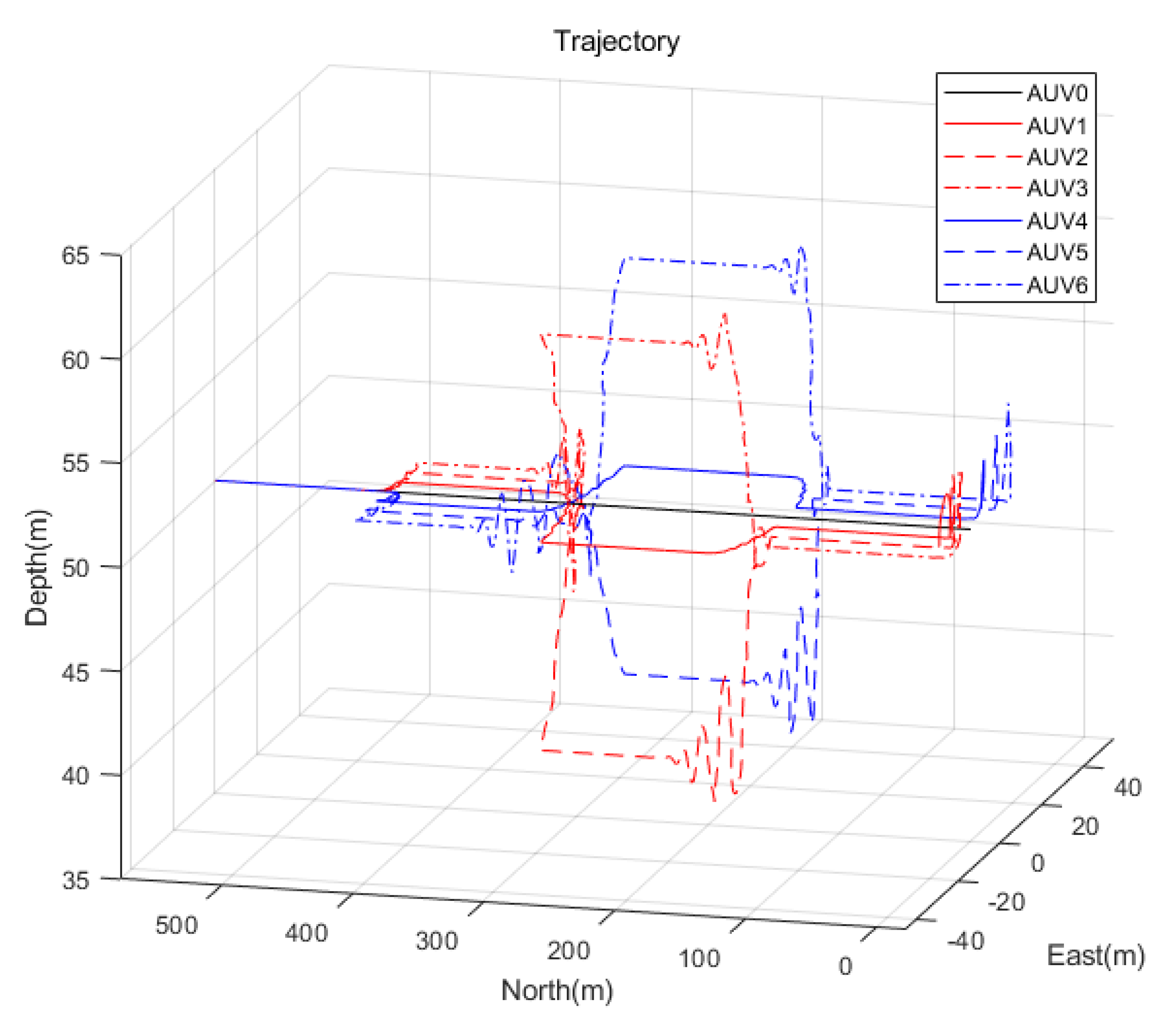
Figure 18. The trajectories of the AUVs (Case 5).

Figure 19. The speeds and angle speeds of the AUVs (Case 5).

Figure 20. The position errors between the AUVs and the target points in the motion coordinate system (Case 5).

The AUV0 sails straight north at a depth of 50 m, while six slave AUVs start tracking AUV0 from different initial positions and switch formations as required. From the tracking trajectories, the six slave AUVs can well complete the formation switching during the tracking process. When a large depth jump occurs in the formation, AUV2 and AUV5 need three fluctuations to complete the formation switching tracking; AUV3 and AUV6 need two fluctuations to achieve the same; AUV1 and AUV4 finish the formation switching tracking relatively smoothly. This indicates that the designed formation switching tracking controller has a high tracking performance.

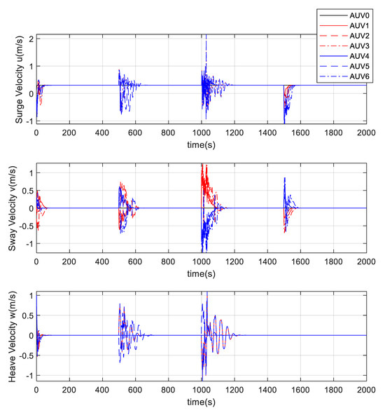
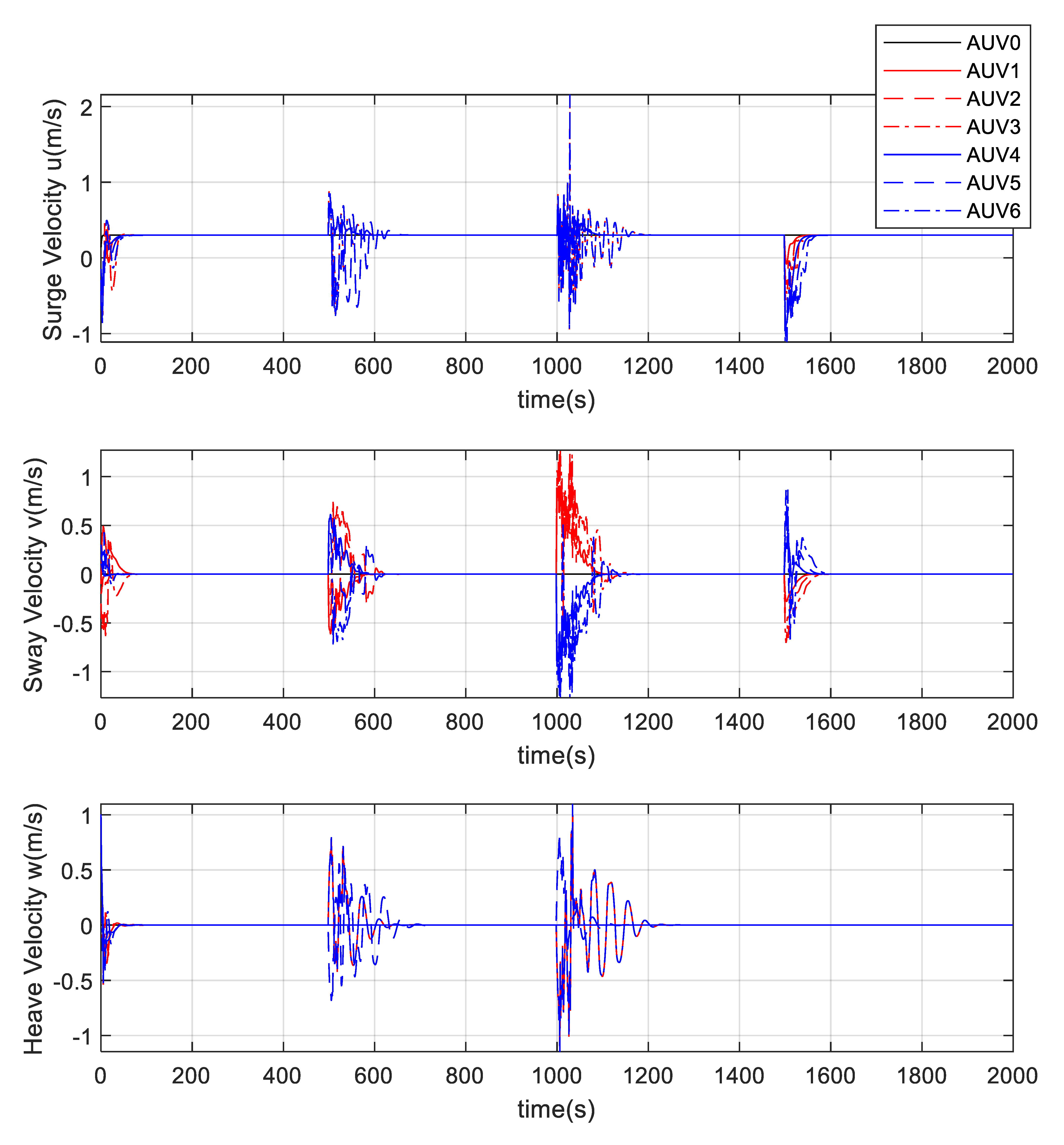
From the velocity change curves, before 50 s, the velocity changes and stabilizes rapidly. This is because the initial positions of the slave AUVs are different, and the slave AUVs adjust their velocity to quickly reach the predetermined trajectory. At 500 s, 1000 s, and 1500 s, the formation of the slave AUV cluster changes and each AUV performs motion adjustments to track its respective desired trajectory. At 500 s, the surge velocity reaches a stable velocity of 0.25 m/s after 120 s, with a maximum value amplitude of 0.75 m/s; the sway velocity decreases to 0 after 120 s, indicating that the slave AUVs have completed the sway motion adjustment for target formation tracking; the heave velocity decreases to 0 after 140 s, demonstrating that the slave AUVs have finished the heave motion adjustment for target formation tracking. At 1000 s, the surge velocity reaches a stable speed of 0.25 m/s after 180 s, with a maximum amplitude of 2.1 m/s (larger than other velocity changes) due to significant jumps in the desired trajectories of AUV5 and AUV6; the sway velocity has a maximum amplitude of 1.2 m/s and decreases to 0 after 130 s; the large fluctuations in sway velocity during this process result from the horizontal position adjustment of each slave AUV; the heave velocity has a maximum amplitude of 1.1 m/s and stabilizes to 0 after 220 s, indicating that each slave AUV conducts heave motion adjustment. At 1500 s, the surge velocity reaches a stable speed of 0.25 m/s after 80 s, with a maximum amplitude of −1.1 m/s; the sway velocity stabilizes to 0 after 85 s; the heave velocity remains unchanged because no depth variation occurs among the AUVs during this process, so only surge and sway motion adjustments are performed. The velocity of each slave AUV can quickly reach a stable value after the formation changes, which indicates that each slave AUV can effectively track the transformed formation.

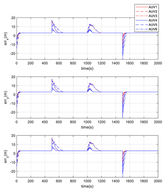
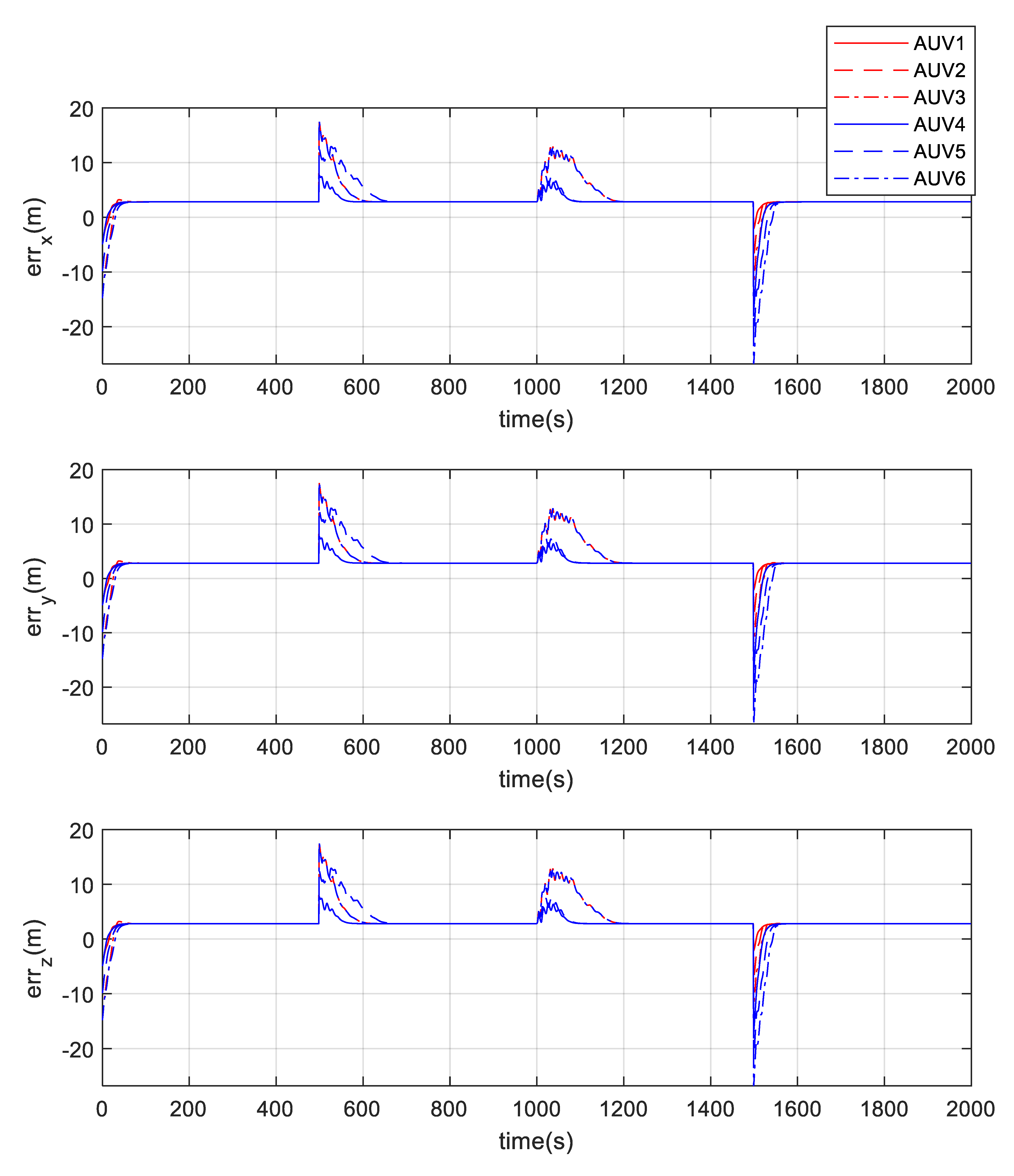
Err_x is the surge error between desired tracking target points near AUV0 and slave AUVs in the motion coordinate system of AUV0; Err_y is the sway error between desired tracking target points near AUV0 and slave AUVs in the motion coordinate system of AUV0; Err_z is the heave error between desired tracking target points near AUV0 and Slave AUVs in the motion coordinate system of AUV0. As analyzed previously, a steady-state error of 2.2 m exists in the surge direction, 2.0 m in the sway direction, and 2.0 m in the heave direction. In this simulation, the Np is 40 and Nc is 2; if Np is increased, the tracking trajectory becomes smoother, but the tracking response slows down and the steady-state tracking error increases; if Np is decreased, the tracking response speeds up and the steady-state tracking error decreases, but the path smoothness deteriorates; if Nc is increased, the tracking response accelerates and the tracking error reduces, yet the control input is prone to oscillation during formation switching. Therefore, reasonable parameter configuration is the key to solving the steady-state tracking error. Throughout the tracking process, when the AUV’s position changes, the error trends in all three directions align with the movement patterns and stabilize rapidly, which demonstrates the effectiveness of the adopted tracking control method.

The centralized MPC tracking control method designed in this study achieves an average QP solution time of approximately 0.14 s for two slave AUVs and about 0.37 s for six slave AUVs. The average QP solution time increases significantly as the number of AUVs grows. This indicates that once the number of AUVs exceeds a certain threshold, the average QP solution time will exceed the sampling period, leading to severe simulation delays and failure to achieve effective tracking. In future research, distributed or decentralized MPC control strategies will be designed to reduce computational load, thereby shortening the average QP solution time for AUV swarms and supporting the feasibility of real-time control in large-scale formations.

6. Verification of Single-AUV Pool Tracking Control Test

In a 50 m × 50 m × 5 m water pool, the designed AUV tracking controller was applied to the experimental equipment, and dynamic straight-line tracking tests based on optical guidance were conducted.

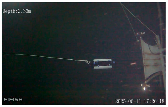
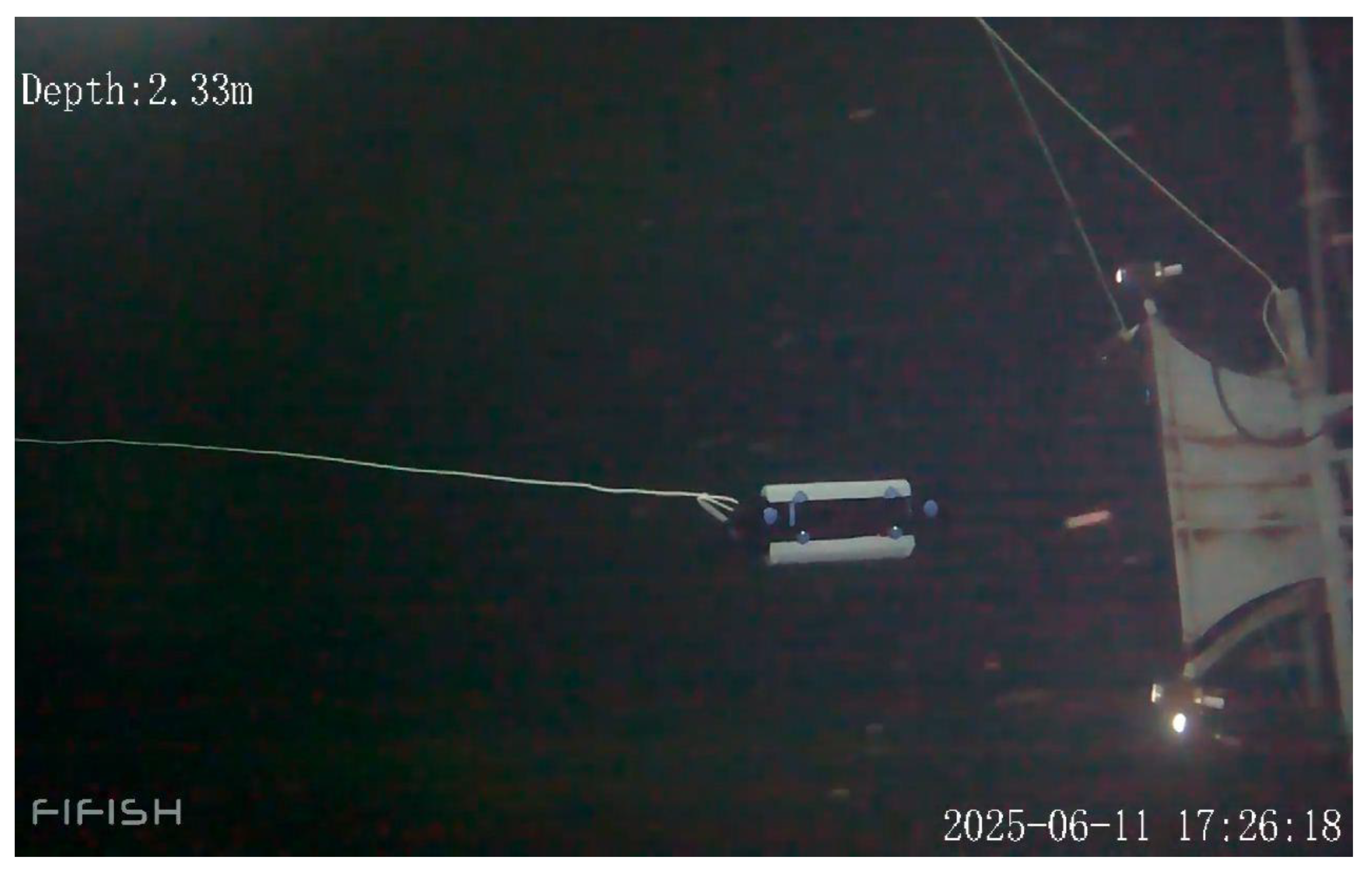
The AUV starts at the water surface, while the tracking target moves forward at a constant speed of 0.5 m/s. The AUV first performs a diving maneuver, submerging to a depth of 1 m. Then, it uses its camera to search for the tracking target. After acquiring the directional position of the tracking target, the AUV adjusts its heading and depth to align itself with the target and maintain the same depth. Then, the AUV moves forward and begins maintaining stable tracking after reaching a certain position behind the target.

The tracking process during the pool test is shown in the Figure 21 below.

Figure 21. The trajectories of the AUV.

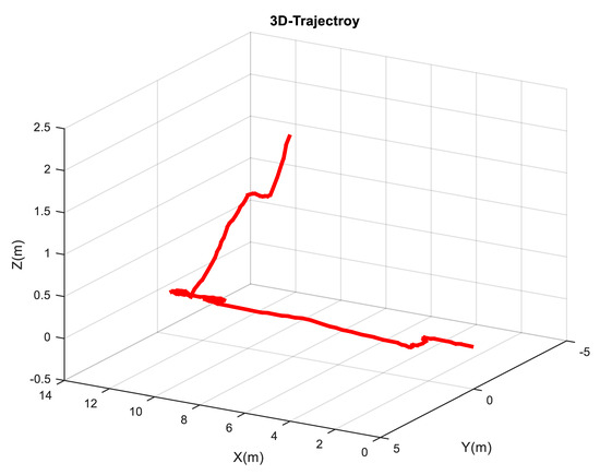
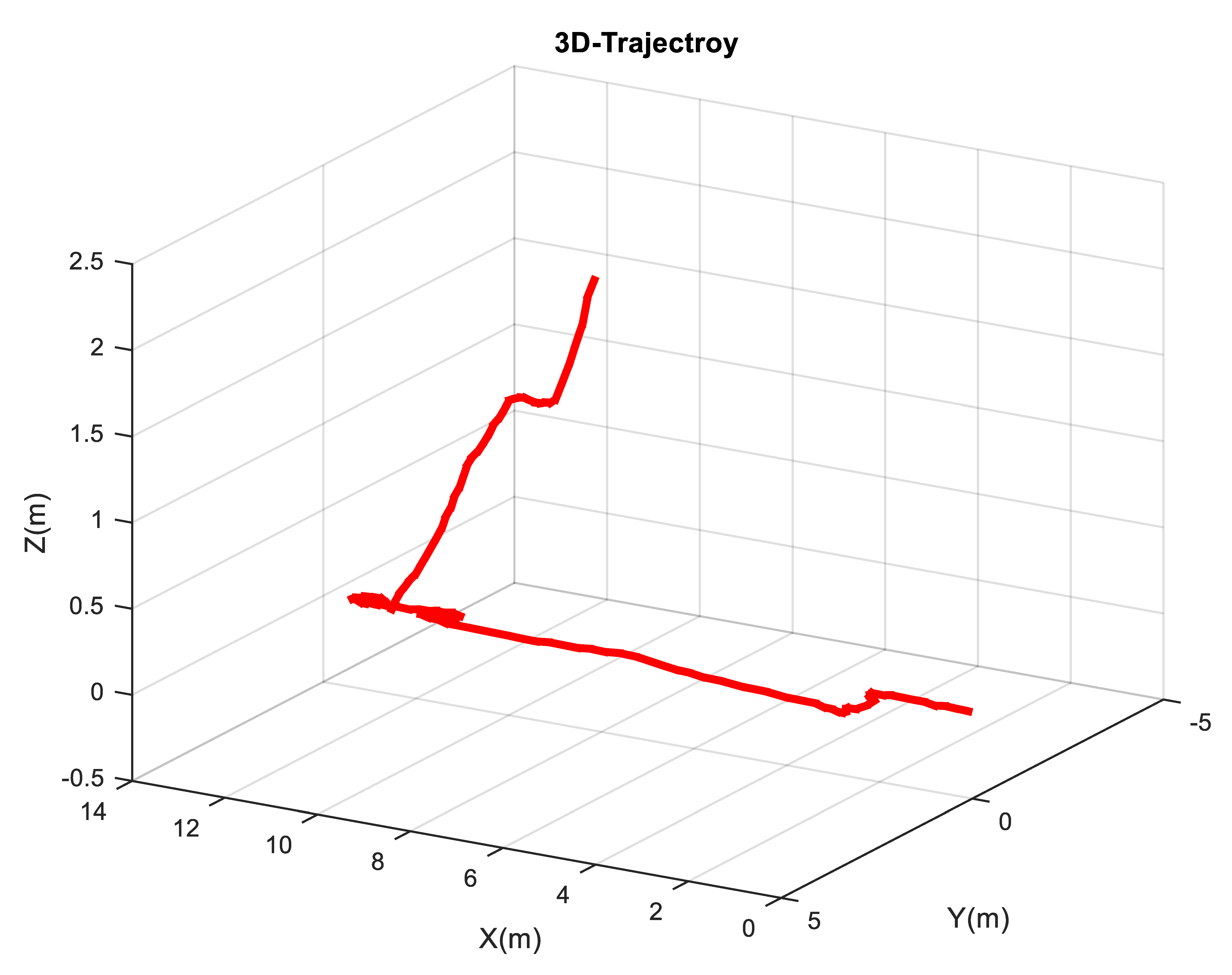
The relative spatial positions of the AUV and the tracking target are shown in the following figure (Figure 22).

Figure 22. The trajectory of the AUV.

From the perspective of the AUV’s relative motion trajectory, during the diving phase, only the AUV’s heading was aligned with the tracking target. As a result, the surge distance gradually expanded from 11 m to approximately 14 m during the descent. After the AUV reached the same depth as the target, it began approaching it, and the surge position error progressively decreased. Throughout this process, sway position changes showed minimal fluctuations, demonstrating the AUV’s effective autonomous tracking adjustment capability.

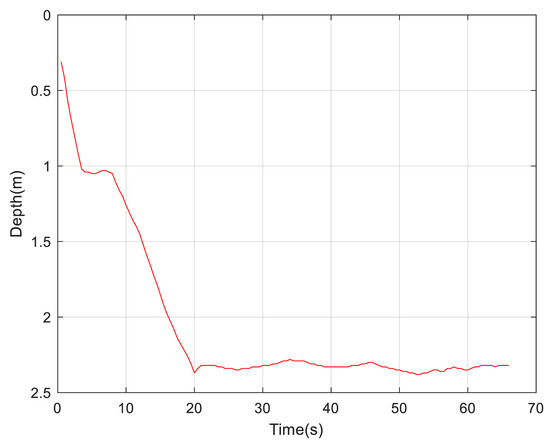
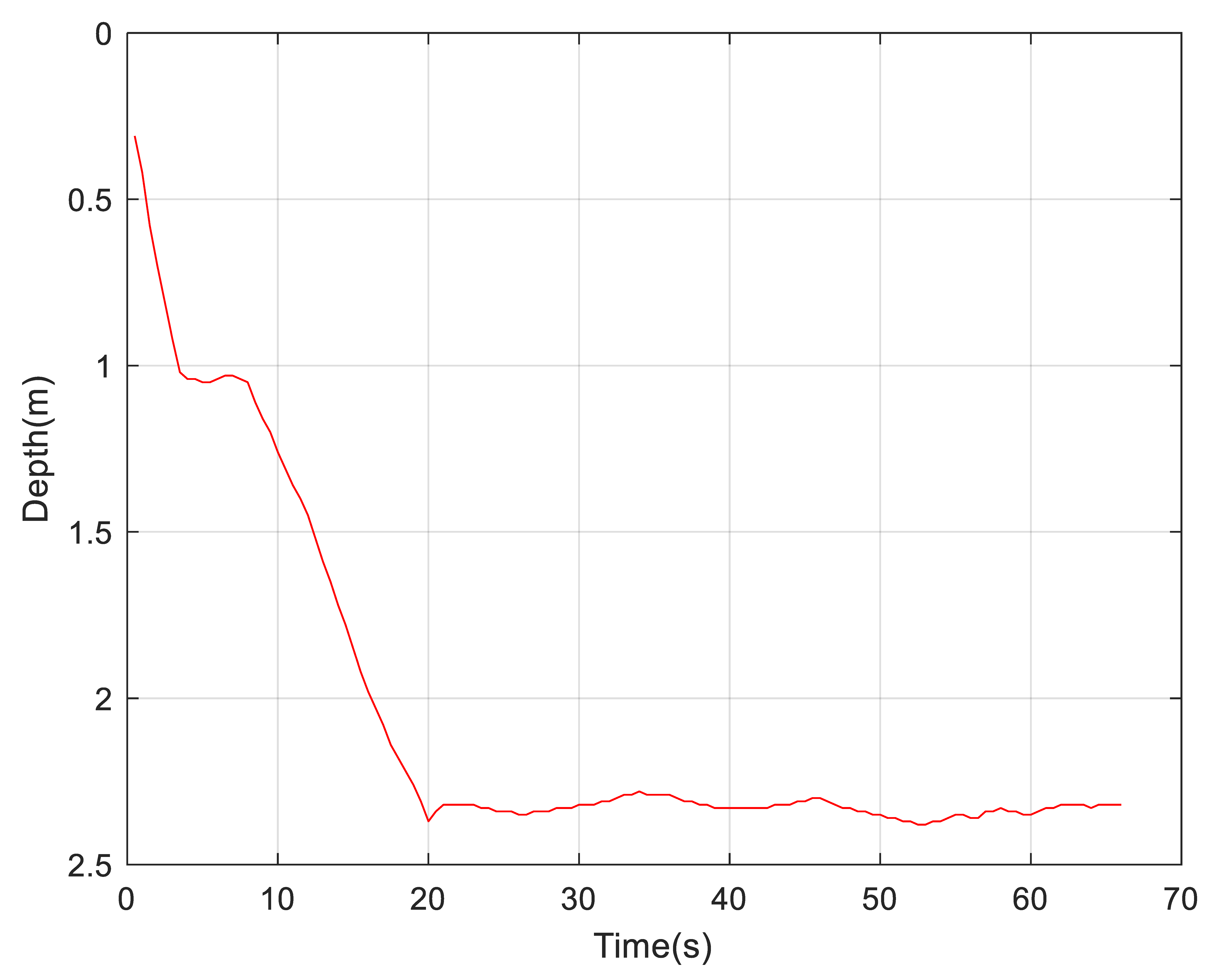
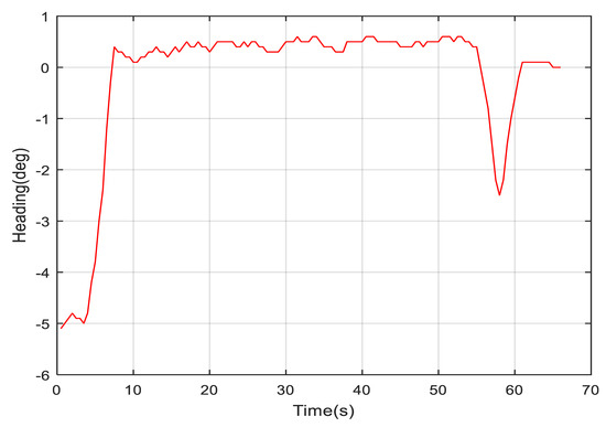
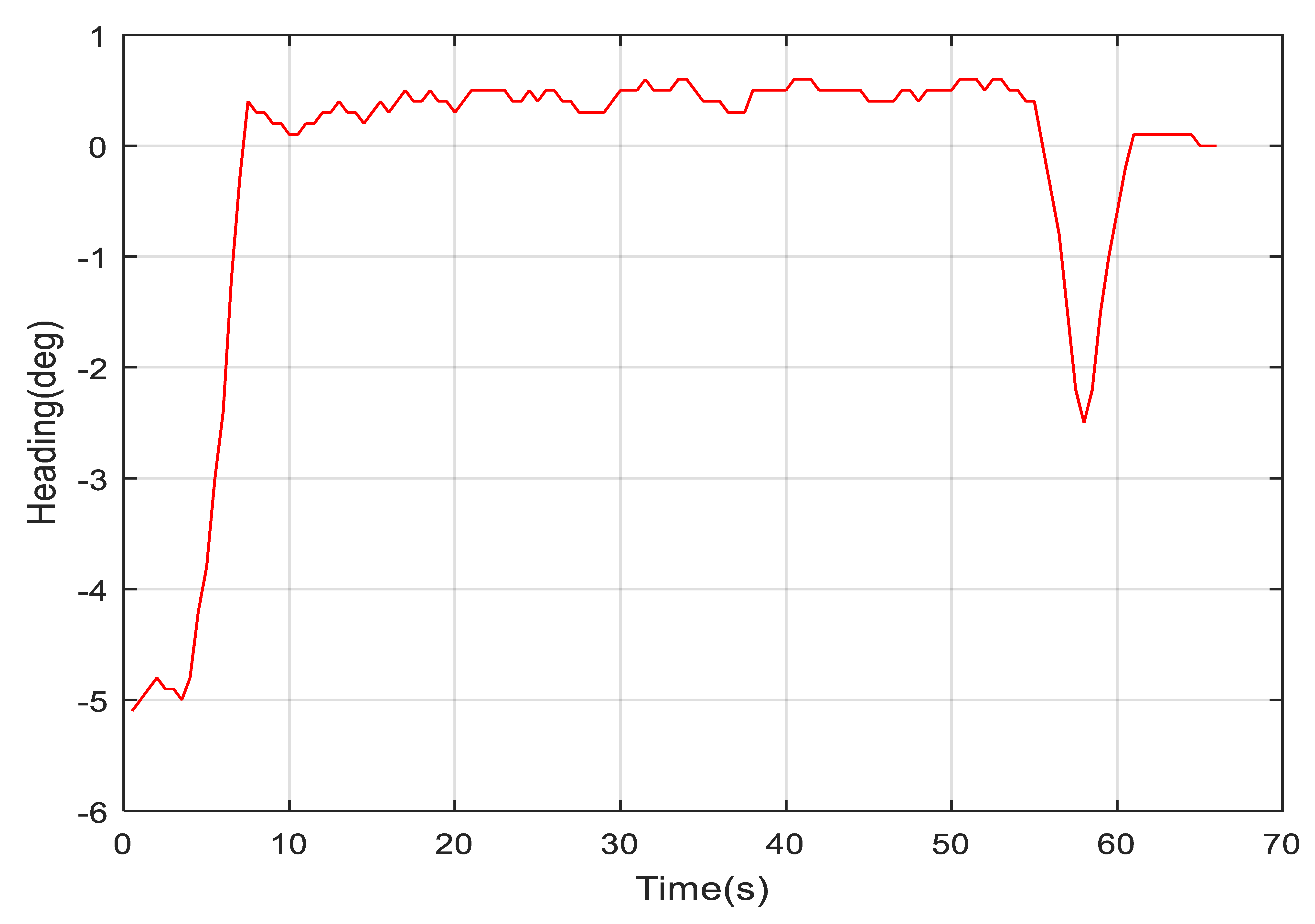
In Figure 23, after 20 s, the AUV’s depth remained consistent with the target and maintain the depth tracking the tracking target. The target depth is 2.33 m; after data analysis, the maximum value of AUV depth error is 0.05 m, and the depth error RMS value is 0.02 m. In Figure 24, after 8 s, the AUV’s heading begins to maintain stable tracking of the tracking target. The target heading is 0 degrees; after data analysis, the maximum value of AUV heading error is 2.5 degrees, and the heading error RMS value is 0.6 degrees.

Figure 23. The error between the AUV and the target of depth.

Figure 24. The error between the AUV and the target of heading.

Based on the depth variation curve and heading error curve, the AUV completed depth adjustment at 20 s, achieving consistency with the target’s depth. Around 8 s, the AUV’s heading error decreased to within 0.5 degrees. After 20 s, the AUV’s depth remained consistent with the target, while a heading adjustment of approximately 3 degrees occurred at 55 s due to course correction when approaching the target. From the overall tracking performance perspective, the AUV successfully achieved the objective of stable tracking.

7. Conclusions

By employing multi-constraint analysis and the MPC method, the various complex constraint issues in the AUV cluster formation transformation and tracking process—including state constraints, collision avoidance and proximity constraints, inherent constraints, and environmental disturbance constraints—were addressed and transformed into state constraints, output constraints, and control input constraints within the predictive model. An MPC normalization approach was then applied to unify all the constraints into control input increment constraints.

Subsequently, an error-augmented model for the AUV and a formation transformation tracking objective optimization function were designed. The constraint conditions were incorporated into this optimization function, leading to the development of a formation transformation tracking controller. Additionally, a segmented formation transformation function was designed based on the trajectory data generated by the leader AUV under control inputs. A series of numerical simulations were conducted, including the following: two follower AUVs tracking the leader on the horizontal plane; two follower AUVs transforming formations during tracking on the horizontal plane; two follower AUVs tracking and transforming formations in three-dimensional space; and six follower AUVs tracking and transforming formations in three-dimensional space. In the second operational scenario, a comparative simulation with the traditional PID control method was performed. Finally, the designed tracking control method was adapted and applied to a pool experiment involving a single AUV tracking a moving target. Analysis of the simulation data demonstrated the effectiveness of the proposed MPC-based cluster formation transformation tracking control method.

This study has certain limitations. During formation transformations, trajectories for the transition process were not designed, resulting in all formation changes occurring instantaneously. This can easily lead to fluctuations in the tracking trajectory during significant formation changes. In subsequent research, considerations for trajectory continuity during formation transformations will be incorporated. Additionally, future work will involve increasing the number of AUVs used in pool experiments to gradually conduct experimental validations of multi-AUV swarm formation transformation and tracking in test pool environments.

References

- Meng, Z.; Liu, S.; Lv, Z. Overview of Multi-AUV Cluster Control Technology. Digit. Ocean. Underw. Warf. 2020, 3, 509–515. [Google Scholar] [CrossRef]
- Wang, S.; Lin, C.; Han, G.; Zhu, S.; Li, Z.; Wang, Z.; Ma, Y. Multi-AUV Cooperative Underwater Multi-Target Tracking Based on Dynamic-Switching-Enabled Multi-Agent Reinforcement Learning. IEEE Trans. Mob. Comput. 2025, 24, 4296–4311. [Google Scholar] [CrossRef] [Scilit]
- Hu, Z.; Ma, C.; Zhang, L.; Halme, A.; Hayat, T.; Ahmad, B. Formation control of impulsive networked autonomous underwater vehicles under fixed and switching topologies. Neurocomputing 2015, 147, 291–298. [Google Scholar] [CrossRef] [Scilit]
- Li, L.; An, R.; Guo, Z.; Gao, J. Multi-AUV Cooperative Search for Moving Targets Based on Multi-Agent Reinforcement Learning. J. Mar. Sci. Eng. 2025, 13, 2072. [Google Scholar] [CrossRef] [Scilit]
- Xu, J.; Wang, M.; Qiao, L.; Zhang, G. Backstepping dynamic sliding mode control for underactuated UUV 3D trajectory tracking. J. Huazhong Univ. Sci. Technol. (Nat. Sci. Ed.) 2015, 43, 107–113. [Google Scholar] [CrossRef]
- Xu, J.; Wang, M.; Qiao, L. Backstepping-based Controller for Three-Dimensional Trajectory Tracking of Underactuated Unmanned Underwater Vehicles. Control Theory Appl. 2014, 31, 1589–1596. [Google Scholar] [CrossRef]
- Raja, R.; Bidyadhar, S. A backstepping approach for the formation control of multiple autonomous underwater vehicles using a leader–follower strategy. J. Mar. Eng. Technol. 2016, 15, 38–46. [Google Scholar] [CrossRef] [Scilit]
- Chen, X.; Liu, Z.; Zhang, J.; Zhou, D.; Dong, J. Adaptive sliding-mode path following control system of the underactuated USV under the influence of ocean currents. J. Syst. Eng. Electron. 2018, 29, 1271–1873. [Google Scholar] [CrossRef] [Scilit]
- Zhang, Y.; Xia, G.; Zhang, W.; Zhang, K.; Yang, H. Decentralized formation cooperative control for homing of a swarm of underactuated AUVs via singular perturbation. Ocean Eng. 2022, 257, 111577. [Google Scholar] [CrossRef] [Scilit]
- Yan, Z.; Zhang, C.; Zhang, M.; Yan, J.; Tian, W. Distributed event-triggered formation control for multi-AUV system via asynchronous periodic sampling control approach. Ocean Eng. 2022, 256, 111561. [Google Scholar] [CrossRef] [Scilit]
- Gao, Z.; Guo, G. Fixed-time Sliding Mode Formation Control of AUVs Based on a Disturbance Observer. IEEE/CAA J. Autom. Sin. 2020, 7, 539–545. [Google Scholar] [CrossRef] [Scilit]
- Liang, H.; Cao, H.; Fu, Y. Decentralized adaptive flocking control algorithm with avoiding collision and preserving connectivity for crowded UUV swarm with uncertainties and input saturation. Ocean Eng. 2021, 237, 109545. [Google Scholar] [CrossRef] [Scilit]
- Deng, S.; Hao, L.; Shen, C. Autonomous Underwater Vehicle (AUV) Motion Design: Integrated Path Planning and Trajectory Tracking Based on Model Predictive Control (MPC). J. Mar. Sci. Eng. 2024, 12, 1655. [Google Scholar] [CrossRef] [Scilit]
- Wang, J.; Zhang, Y.; Ren, S.; Wang, H. Parameter Optimization Design of MPC Controller in AUV Motion Control Based on Improved Black-Winged Kite Algorithm. J. Mar. Sci. Eng. 2025, 13, 2018. [Google Scholar] [CrossRef] [Scilit]
- Zhang, W.; Yu, C.; Teng, Y. Research on UUV Path Following Control Based on Model Predictive Control. Chin. J. Sci. Instrum. 2017, 38, 2659–2666. [Google Scholar]
- Zhang, W.; Teng, Y.; Wei, S.; Xiong, H.; Ren, H. The robust H-infinity control of UUV with Riccati equation solution interpolation. Ocean Eng. 2018, 156, 252–262. [Google Scholar] [CrossRef] [Scilit]
- Zhang, W.; Teng, Y.B.; Chen, H.T.; Yu, C.X. On the robust model predictive control method of dynamic positioning to line for UUV recovery. In Proceedings of the OCEANS 2016 MTS/IEEE Monterey, Monterey, CA, USA, 19–23 September 2016; pp. 1–6. [Google Scholar] [CrossRef] [Scilit]
- Teng, Y.; Liu, Z.; Zhang, L.; Liu, C.; Wei, N. On Intelligent Ship Tracking Control Method Based on Hierarchical MPC. In Proceedings of the 40th Chinese Control Conference, Shanghai, China, 26–28 July 2021; pp. 1–6. [Google Scholar] [CrossRef] [Scilit]
- Dai, L.; Zhang, D.; Wang, S.; Nie, G.; Zhu, X.; Wang, X. Trajectory Tracking Control of an Autonomous Underwater Vehicle Under Disturbance and Model Uncertainty. J. Mar. Sci. Eng. 2025, 13, 2210. [Google Scholar] [CrossRef] [Scilit]
- Zhang, Y.; Liu, X.; Luo, M.; Yang, C. MPC-based 3-D trajectory tracking for an autonomous underwater vehicle with constraints in complex ocean environments. Ocean Eng. 2019, 189, 106309. [Google Scholar] [CrossRef] [Scilit]
Disclaimer/Publisher’s Note: The statements, opinions and data contained in all publications are solely those of the individual author(s) and contributor(s) and not of MDPI and/or the editor(s). MDPI and/or the editor(s) disclaim responsibility for any injury to people or property resulting from any ideas, methods, instructions or products referred to in the content. |
© 2025 by the authors. Licensee MDPI, Basel, Switzerland. This article is an open access article distributed under the terms and conditions of the Creative Commons Attribution (CC BY) license.