Cavitation Coefficient Identification Model for an Axial Flow Pump Based on Pressure Signal Feature Extraction and Spider Wasp Optimization Algorithm

Abstract

This research proposes a quantitative cavitation-coefficient identification method based on a VMD-SWO-BiLSTM model, addressing the current limitations of existing machine-learning-based cavitation diagnostics, which mainly classify cavitation stages rather than identify the cavitation coefficient as a continuous quantity. Pressure fluctuation signals under various cavitation conditions are decomposed using Variational Mode Decomposition (VMD), and sample entropy is extracted to represent signal complexity. The Spider Wasp Optimization (SWO) algorithm optimizes the hyperparameters of a BiLSTM network, forming a composite VMD-SWO-BiLSTM framework. Multi-point input features from unsteady internal flow simulations and experimental measurements are used for model training and validation. Results show that the proposed model outperforms conventional BiLSTM, achieving mean absolute percentage error below 5% based on multi-point pressure signals. Validation with eight experimental datasets yields a maximum absolute error of 0.006 and a maximum percentage error of 4.7%. The proposed method can be applied to online monitoring and intelligent diagnosis of cavitation in axial flow pumps.

1. Introduction

The axial-flow pump transports fluid in the axial direction by means of a rotating impeller, making it suitable for applications involving large flow rates and low heads. In practical operation, axial flow pumps are frequently subjected to cavitation, which induces undesirable flow patterns and significant pressure fluctuations within the pump system. In severe cases, cavitation can lead to physical damage to the pump components and pose a threat to operational safety.

In recent years, significant progress has been made in understanding cavitation evolution and its impact on pump flow fields [1,2,3]. Gong et al. [4] used synchronized experiments to study cavitation scale evolution and its effect on pump performance. Jia et al. [5] examined early-stage cavitation in centrifugal pumps, establishing quantitative relations between cavitation number, pressure pulsation, and fluid forces. Du et al. [6] investigated leading-edge cavitation characteristics in double-suction centrifugal pumps, showing the influence of inlet flow rate and blade pressure distribution. Wu et al. [7] highlighted the correlation between vortices and cavitating flows using the Zwart-Gerber-Belamri model. Li et al. [8] analyzed energy dissipation induced by tip leakage vortex cavitation, identifying turbulent dissipation as the primary source of energy loss.

Beyond the investigation of cavitation phenomena, numerous approaches have been explored for the detection and assessment of cavitation severity. Cao et al. [9] proposed an analytical method using vibration signal features to detect cavitation. Al-Obaidi et al. [10] combined vibration and acoustic techniques for cavitation diagnosis, while Cao et al. [11] utilized wavelet packet transform to process vibration signals and proposed an unequal interval weight grey (UIWG) model to reconstruct the functional relationship between cavitation and vibration, enabling identification of cavitation stages in centrifugal pumps. Lan et al. [12] developed an MLP-Mixer framework to assess cavitation intensity in axial piston pumps. Fecser et al. [13] studied cavitation onset in centrifugal pumps via simulations and experiments. Huang et al. [14] applied singular value decomposition and hierarchical clustering for cavitation fault diagnosis. Chen et al. [15] demonstrated that Variational Mode Decomposition (VMD) components provide more informative cavitation signals than Empirical Mode Decomposition (EMD).

With the rapid advancement of artificial intelligence (AI), machine-learning, and deep-learning techniques have been increasingly applied to flow field and cavitation analysis [16,17,18]. Tong et al. [19] developed a GPU-accelerated approach combining a Convolutional Neural Network-based Autoencoder (CNN-AE) for spatial feature extraction and a Long Short-Term Memory (LSTM) network for temporal dynamics to predict turbomachinery flows. Li et al. [20] applied deep learning models optimized with the Northern Goshawk optimization algorithm to predict stall and surge in axial compressors under distorted inlet conditions. In cavitation detection, Dong et al. [21] proposed a multi-resolution cavitation state identification method using Wavelet Packet Decomposition (WPD) to extract vibration features as inputs for neural networks. Matloobi et al. [22] applied an Artificial Immune Network (AIN) using time-frequency features of vibration and current signals to identify cavitation. Tan et al. [23] combined Stacked Autoencoders (SAE), LSTM, and CNN to classify normal, slight, and severe cavitation states in a mixed-flow pump. Gaisser et al. [24] employed Convolutional Neural Networks (CNN) to analyze acoustic emissions from hydraulic machinery for cavitation detection. Kamali et al. [25] studied ventilated cavitation states behind disk-type cavitators using experiments, numerical simulations, and machine learning to predict cavitation length and classify cavitation states. Li et al. [26] combined Complete Ensemble Empirical Mode Decomposition with Adaptive Noise (CEEMDAN) and Particle Swarm Optimization–Support Vector Machine (PSO-SVM) for cavitation feature extraction and classification in canned motor pumps. Wu et al. [27] integrated experiments, numerical simulations, and neural networks to investigate anomalous peak values under critical cavitation conditions in mixed-flow pipeline pumps. Liu et al. [28] extracted Root Mean Square (RMS) and kurtosis features from vibration signals and trained a two-layer back-propagation neural network for cavitation state classification in centrifugal pumps. Wang et al. [29] developed a Dual-Path Attention Mechanism with Correlation Alignment (DPAM-CORAL) method to identify cavitation intensity in an axial piston pump using measured pressure signals.

Despite these advances, intuitively assessing cavitation in axial-flow pumps remains challenging. Cavitation significantly affects local pressure fluctuations, which are nonlinear and non-stationary. Most previous studies focus on vibration and acoustic signals, with limited work on axial-flow pumps. Therefore, developing a pressure-fluctuation-based method for cavitation coefficient identification is crucial to avoid critical cavitation and enhance operational stability. Effectively extracting features and constructing a reliable identification model remains a key technical challenge. Table 1 presents an overview of current cavitation detection methods and the proposed approach.

Table 1. Comparison of existing cavitation detection methods and the proposed model.

Category	Pump Type	Identification Method
Current-signal-based detection [15]	Mostly centrifugal pumps	Signal analysis
Vibration-based detection [22]	Mostly centrifugal pumps	Neural-network models
Acoustic-based detection [24]	Mostly centrifugal pumps	Neural-network models
Pressure-based detection [23,29]	Centrifugal, mixed-flow, piston pumps	Neural-network models
Proposed method (Pressure-based)	Axial-flow pumps	VMD-SWO-BiLSTM

In this study, a cavitation coefficient identification model for an axial flow pump system is proposed based on a Bidirectional Long Short-Term Memory (BiLSTM) neural network optimized by the Spider Wasp Optimization (SWO) algorithm. The model first employs Variational Mode Decomposition (VMD) to perform multiscale decomposition of pressure fluctuation signals measured at different locations. Frequency-domain analysis is then used to extract feature information from each intrinsic mode function (IMF), and sample entropy is calculated to obtain complexity-representative features as input to the neural network. The BiLSTM network, capable of capturing bidirectional temporal dependencies in time series, enhances the model’s ability to learn nonlinear evolution patterns in pressure fluctuation signals. To further improve the performance, the SWO algorithm is introduced to optimize key hyperparameters of the BiLSTM model. A comparative analysis was conducted between the optimized model and the unoptimized BiLSTM model in terms of cavitation coefficient identification accuracy. In addition, this study compares the identification accuracy using data from different measurement points. Finally, the reliability of the model is validated through experimental data. The results demonstrate that the proposed VMD-SWO-BiLSTM model exhibits high identification accuracy and strong robustness in identifying cavitation coefficients of axial flow pumps. This approach effectively enhances identification accuracy, providing a practical tool for online monitoring and intelligent diagnosis of cavitation in axial flow pumps.

2. Research Process

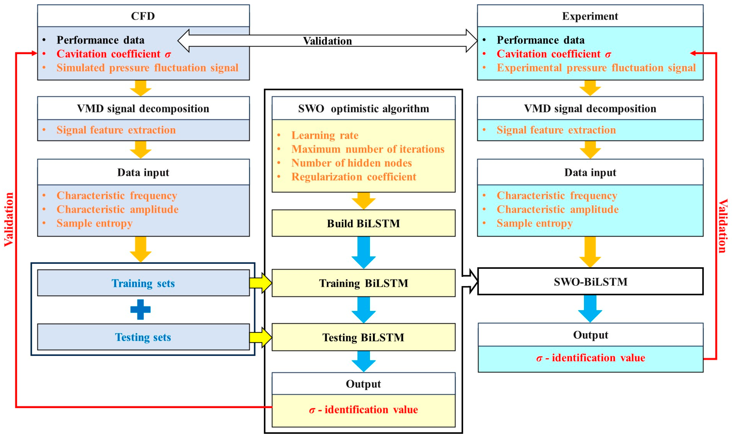
The research procedure for constructing the VMD-SWO-BiLSTM model is as follows:

Given the limited number of samples obtained from experiments, computational fluid dynamics (CFD) simulations were first employed to generate pressure fluctuation signals at various monitoring points of the axial flow pump under different cavitation coefficients for a given flow condition. The arrangement of monitoring points in the simulation matched that in the physical experiments. Additionally, the external characteristics and cavitation performance curves derived from the simulations were compared with experimental data to verify the reliability of the numerical model.

Under different cavitation conditions, the pressure fluctuation signals inside an axial-flow pump typically exhibit strong nonlinear and non-stationary characteristics. This research employs the Variational Mode Decomposition (VMD) method to decompose and extract the multiscale features of the pressure fluctuation signals. VMD allows the original signals to be decomposed into intrinsic mode functions, effectively isolating frequency components associated with cavitation. Sample Entropy was then calculated for each mode to quantify its complexity, providing robust and discriminative features that reflect cavitation-induced irregularities. The combination of VMD and Sample Entropy provided clearer feature separability and higher identification stability, particularly under limited dataset size and noise contamination.

Based on the extracted features, a sample dataset was constructed and divided into training and testing sets. To improve upon the conventional LSTM architecture, a Bidirectional LSTM (BiLSTM) network was employed, enabling the model to simultaneously incorporate past and future temporal information in the feature sequences. This capability allows the model to more accurately capture the evolution patterns of pressure fluctuation features with varying cavitation intensities, thereby significantly enhancing identification precision.

To further improve model expressiveness, the Spider Web Optimization (SWO) algorithm was utilized to optimize key hyperparameters, including the maximum training iterations, learning rate, number of hidden neurons, and regularization coefficient. Inspired by the vibration-based prey-locating behavior of spiders, the SWO algorithm achieves rapid and global optimization in high-dimensional parameter spaces, effectively avoiding local optima. Its integration into neural network tuning enhances convergence speed and generalization performance, enabling more robust handling of noise and non-stationary characteristics in the pressure fluctuation signals.

Model training was then conducted using the training set, and the identification error on the testing set was evaluated. A comparative analysis of recognition performance using data from different monitoring points was also carried out to optimize input selection, improving both model adaptability and overall identification accuracy. Finally, pressure fluctuation signals obtained from experiments were processed for feature extraction and input into the trained VMD-SWO-BiLSTM model to validate its reliability and applicability in real engineering scenarios.

The overall research framework of the proposed VMD-SWO-BiLSTM model for cavitation coefficient identification in the axial flow pump is illustrated in Figure 1.

Figure 1. Research methodology of the proposed VMD-SWO-BiLSTM model for cavitation coefficient identification in the axial flow pump.

3. Test Device

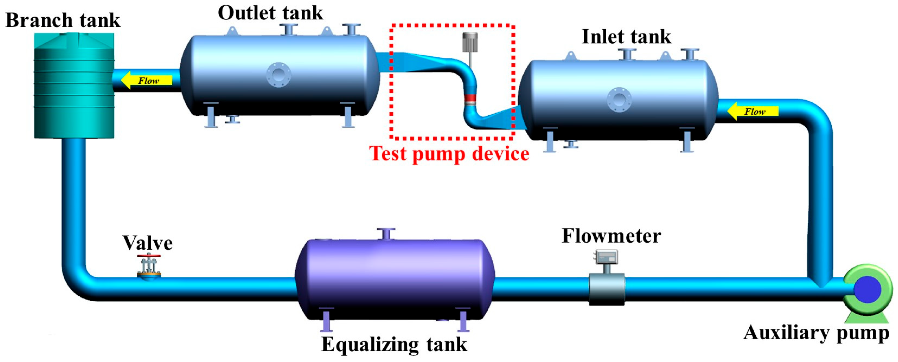
The cavitation experiment of the axial flow pump device was conducted on a high-precision hydraulic machinery test bench, as illustrated in Figure 2. The test bench was equipped with auxiliary pumps and flow meters for flow control and monitoring. Relevant acquisition equipment was utilized to collect data on the pump head, rotational speed, torque, and pressure fluctuation signals during operation.

Figure 2. High-precision hydraulic machinery test bench used for cavitation experiments of the axial flow pump.

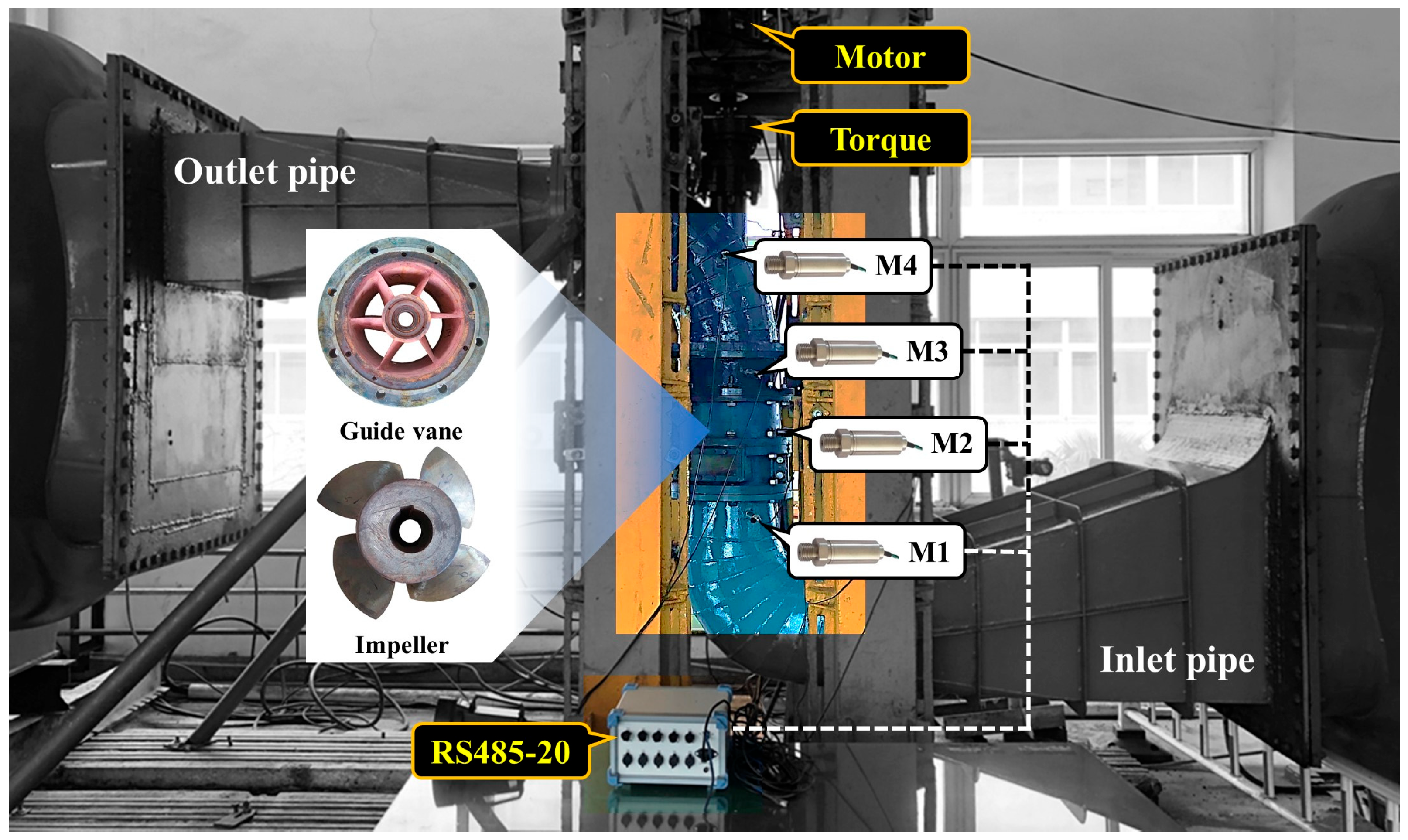
The vertical axial flow pump model consisted of an inlet conduit, an outlet conduit, an impeller, and guide vanes. The impeller included four blades, with a diameter of 300 mm and a hub ratio of 0.45. The rated rotational speed was 1300 rpm. The guide vane section was composed of six blades. The test apparatus was equipped with pressure fluctuation sensors and an RS485-20 signal acquisition device(LST Instrument and Instrumentation Limited Company, Qingdao, China), as shown in Figure 3. Four pressure sensors were threaded and fixed onto the outer casing of the experimental setup. Sensor M1 was positioned at the impeller inlet, sensor M2 at the guide vane inlet, sensor M3 at the guide vane outlet, and sensor M4 at the outlet elbow. The shaft rotational speed and torque were measured using a torque meter installed between the motor and the pump shaft.

Figure 3. The experimental axial flow pump setup.

The head of the axial flow pump device was calculated based on the Bernoulli equation:

$$H={\displaystyle \frac{P_{\mathrm{out}}-P_{\mathrm{in}}}{\rho g}}+{\displaystyle \frac{u_{\mathrm{out}}^2-u_{\mathrm{in}}^2}{2g}}+(z_{\mathrm{out}}-z_{\mathrm{in}})$$

(1)

where $P_{\mathrm{out}}$ represents the average static pressure at the outlet cross-section of the outlet conduit, while $P_{\mathrm{in}}$ denotes the average static pressure at the inlet cross-section of the inlet conduit. $z_{\mathrm{out}}$ and $z_{\mathrm{in}}$ are the distances from the outlet cross-section and the inlet cross-section to the measurement datum, respectively, while $u_{\mathrm{out}}$ and $u_{\mathrm{in}}$ are the flow velocities at the outlet and inlet cross-sections. $\rho$ is the density of water, and g is the local gravitational acceleration.

The shaft power P was determined using Equation (2), and the efficiency η of the axial flow pump was calculated using Equation (3).

$$P={\displaystyle \frac{\pi n\left(T+T_0\right)}{30}}$$

(2)

$$\eta ={\displaystyle \frac{\rho gQH}{P}}\times 100\%$$

(3)

where n denotes the impeller rotational speed, T is the output torque of the pump shaft, $T_0$ is the no-load torque, and Q represents the flow rate.

The system uncertainty in the model experiment was $U_S=\pm \left(\sqrt{{U_h}^2+{U_f}^2+{U_r}^2+{U_t}^2}\right)=\pm 0.29\%$. Specifically, the uncertainty of the head measurement was $U_h=\pm 0.10\%$, the flow rate was $U_f=\pm 0.22\%$, the rotational speed $U_r=\pm 0.05\%$, and the torque $U_t=\pm 0.15\%$. The random uncertainty $U_R$ was obtained through ten repeated experiments under the same flow condition and was determined to be $\pm 0.18\%$. Therefore, the total uncertainty of the experimental system was $U_T=\pm \left(\sqrt{{U_S}^2+{U_R}^2}\right)=\pm 0.34\%$.

The cavitation experiment was carried out according to the following procedure:

Step 1: Start the auxiliary pump and adjust the flow control valves until the target flow rate is reached. The flow rate is measured by a DN400 electromagnetic flowmeter, and its uncertainty is evaluated at both the inlet and outlet. The axial-flow pump is then operated at the rated rotational speed of 1300 rpm, monitored by the JC torque meter. Once the flow rate, head, torque, and rotational speed remain stable, the baseline non-cavitating condition is recorded.

Step 2: Cavitation is induced by gradually reducing the inlet absolute pressure through the inlet valve. The inlet pressure is measured using an absolute pressure transmitter. At each pressure level, the flow rate is maintained constant, and the system is allowed to reach steady state before data acquisition.

Step 3: For each inlet pressure step, the pump head is obtained from the inlet and outlet pressure readings, while the torque and shaft speed are collected using the JC torque meter. The net positive suction head (NPSH) is calculated from the measured inlet absolute pressure. Pressure fluctuation signals are synchronously recorded at the four monitoring points using the RS485-20 acquisition system. The sensors are located at the impeller inlet (M1), guide vane inlet (M2), guide vane outlet (M3), and outlet elbow (M4).

Step 4: As the inlet pressure decreases, cavitation development is evaluated based on the variation in pump head, the increase in pressure fluctuation amplitudes, and the appearance of cavitation-induced instabilities. The critical cavitation condition is identified at the 3% head-drop point.

Step 5: Before severe cavitation causes operational instability, the pressure reduction process is stopped. The inlet pressure is gradually restored to normal conditions, after which the pump is safely shut down. This procedure ensures repeatability and protects the test apparatus from damage.

4. Numerical Simulation

4.1. Calculation Method

In this study, the internal flow of the axial flow pump device was simulated using ANSYS CFX 19.0. For the cavitation simulation, a homogeneous two-phase flow model was adopted, in which the liquid water was assumed to be incompressible and Newtonian, and interphase heat transfer was neglected. The internal flow of the axial-flow pump device was assumed to be turbulent and unsteady to capture the flow pulsation and instability that actually occur under cavitating conditions. The turbulence model employed was the Shear Stress Transport k-ω (SST k-ω) model, which is capable of effectively capturing large curvature separation flows typically observed in axial flow pumps [30]. The governing equations for turbulent kinetic energy k and specific dissipation rate ω are expressed as follows:

$${\displaystyle \frac{\partial (\rho k)}{\partial t}}+{\displaystyle \frac{\partial (\rho k{u}_j)}{\partial x_j}}={\displaystyle \frac{\partial }{\partial x_j}}\left[{\mathsf{\Gamma }}_k{\displaystyle \frac{\partial k}{\partial x_j}}\right]+G_k-Y_k+S_k$$

(4)

$${\displaystyle \frac{\partial (\rho \omega )}{\partial t}}+{\displaystyle \frac{\partial (\rho \omega u_j)}{\partial x_j}}={\displaystyle \frac{\partial }{\partial x_j}}\left[{\mathsf{\Gamma }}_{\omega }{\displaystyle \frac{\partial \omega }{\partial x_j}}\right]+G_{\omega }-Y_{\omega }+S_{\omega }$$

(5)

where $G_k$ is the production term of $k$, $G_{\omega }$ is the production term of $\omega$, $Y_k$ is the dissipation term of $k$, $Y_{\omega }$ is the dissipation term of $\omega$, $S_k$ and $S_{\omega }$ are custom source terms.

The cavitation model employed in the numerical simulation was the ZGB (Zwart-Gerber-Belamri) model. This model is established on the mechanical laws of bubble growth and collapse, assuming spherical bubbles with a uniformly distributed bubble number density [31]. It is widely used in cavitation simulations of pumps, helping to achieve stable calculations and accurately predict head-drop characteristics and cavitation inception. The expression of the ZGB cavitation model is [32]:

$$m=\left\{\begin{array}{cc}{F}_{vap}{\displaystyle \frac{3a_{nuc}\left(1-a_V\right){\rho }_V}{R_B}}\sqrt{{\displaystyle \frac{2\left(P_V-P\right)}{3{\rho }_l}}},\hfill & P\le P_V\\ F_{cond}{\displaystyle \frac{3a_V{\rho }_V}{R_B}}\sqrt{{\displaystyle \frac{2\left(P-P_V\right)}{3{\rho }_l}}},\hfill & P>P_V\end{array}\right.$$

(6)

where $a_{nuc}$ is the volume fraction of the cavity core, and the value is $5\times {10}^{-4}$. $a_V$ is the vapor volume fraction, $a_V={\displaystyle \frac{4}{3}}\pi R_B^3{N}_B$. $N_B$ is the number of bubbles per unit volume of the water. $R_B$ is the radius of the bubbles, and the value is $1\times {10}^{-6}$ m. $P_V$ represents the saturation pressure of the vapor, which is set to 3574 Pa. $F_{vap}$ denotes the evaporation coefficient, and the value is 50. $F_{cond}$ denotes the condensation coefficient, and the value is 0.01.

The cavitation conditions are described by the cavitation coefficient, which is determined by the following formula:

$$\sigma ={\displaystyle \frac{P-P_V}{0.5\rho u^2}}$$

(7)

where u is the circumferential velocity of the impeller outlet section, m/s. P represents the total pressure at the inlet, Pa. $P_V$ represents the saturation pressure, Pa.

4.2. Boundary Conditions and Mesh Generation

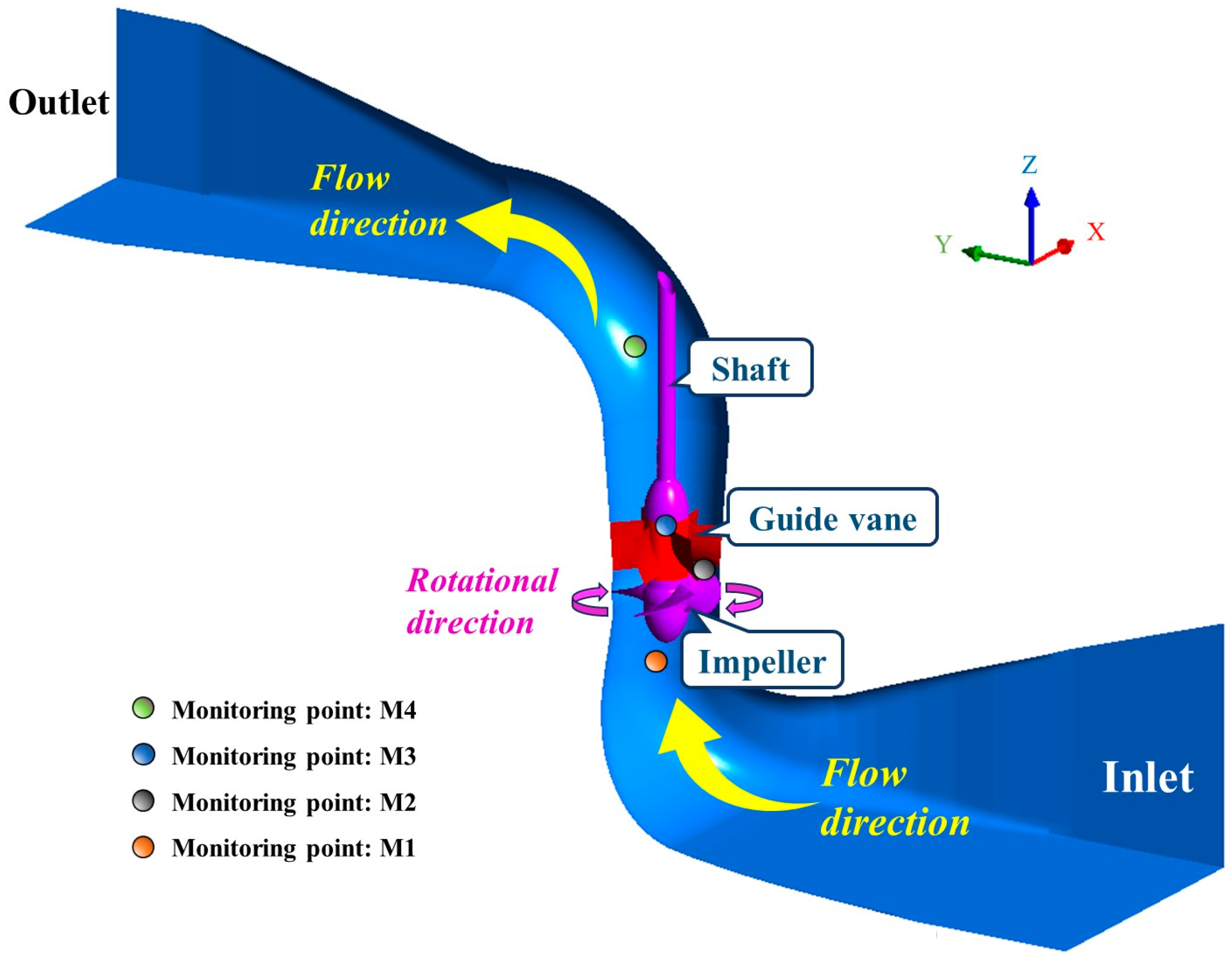
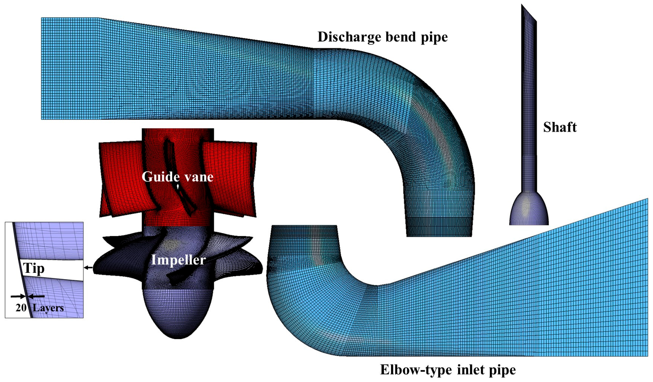
The 1:1 three-dimensional geometry of the experimental pump apparatus was constructed using UG 12.0. To ensure the consistency of data for subsequent validation, the monitoring points in the numerical simulation of the flow field were arranged in accordance with the sensor layout in the experimental setup. In the unsteady simulations, four monitoring points were placed near the inner wall of the pump casing: M1 was located at the impeller inlet, M2 at the guide vane inlet, M3 at the guide vane outlet, and M4 at the outlet elbow. The geometric model and its components are illustrated in Figure 4.

Figure 4. Computational domain model of the axial flow pump device with monitoring points corresponding to the sensor locations in the experiment.

The inlet of the pump device is set as a total pressure boundary. The outlet boundary condition is set to a mass flow rate. All walls of the physical model are specified as smooth no-slip walls based on the fundamental assumption of viscous fluid mechanics. This assumption is essential for accurately resolving the boundary layer, capturing near-wall velocity gradients, and correctly predicting shear stress and pressure distribution. The fluid medium in cavitation computation consists of water and vapor at 25 °C, and the saturation pressure is defined as 3574 Pa. For steady-state calculations, dynamic-static interfaces within the domain are modeled as frozen rotor, whereas unsteady-state simulations are configured as transient rotor-stator with a time step of $1.3\times {10}^{-4}$ s, matching the time required for the impeller to rotate by 1°. The convergence criterion is set to an RMS residual of $1\times {10}^{-5}$. All unsteady simulations use the results from steady-state simulations as initial conditions to save computational resources. For each computational case, eight revolutions of the impeller were simulated. The final results are taken from the last three rotational cycles after the computation reaches stabilization.

A high-quality mesh is crucial for accurately capturing the flow field characteristics of cavitation in a pump. To achieve this, structured hexahedral meshes were created for the inlet and outlet flow passages using ICEM 19.0, while Turbogrid 19.0 was employed to generate structured meshes for the impeller and guide vane. Local refinement was implemented in critical areas of the pump, particularly at the impeller tip clearance, where 20 layers of boundary layer mesh were applied. Different mesh configurations were developed with cell counts of 3.98 million, 4.66 million, 6.03 million, 7.83 million, 9.76 million, 10.63 million, and 11.84 million. The mesh configuration containing 10.63 million cells is presented in Figure 5.

Figure 5. Detailed mesh configuration of the axial flow pump device.

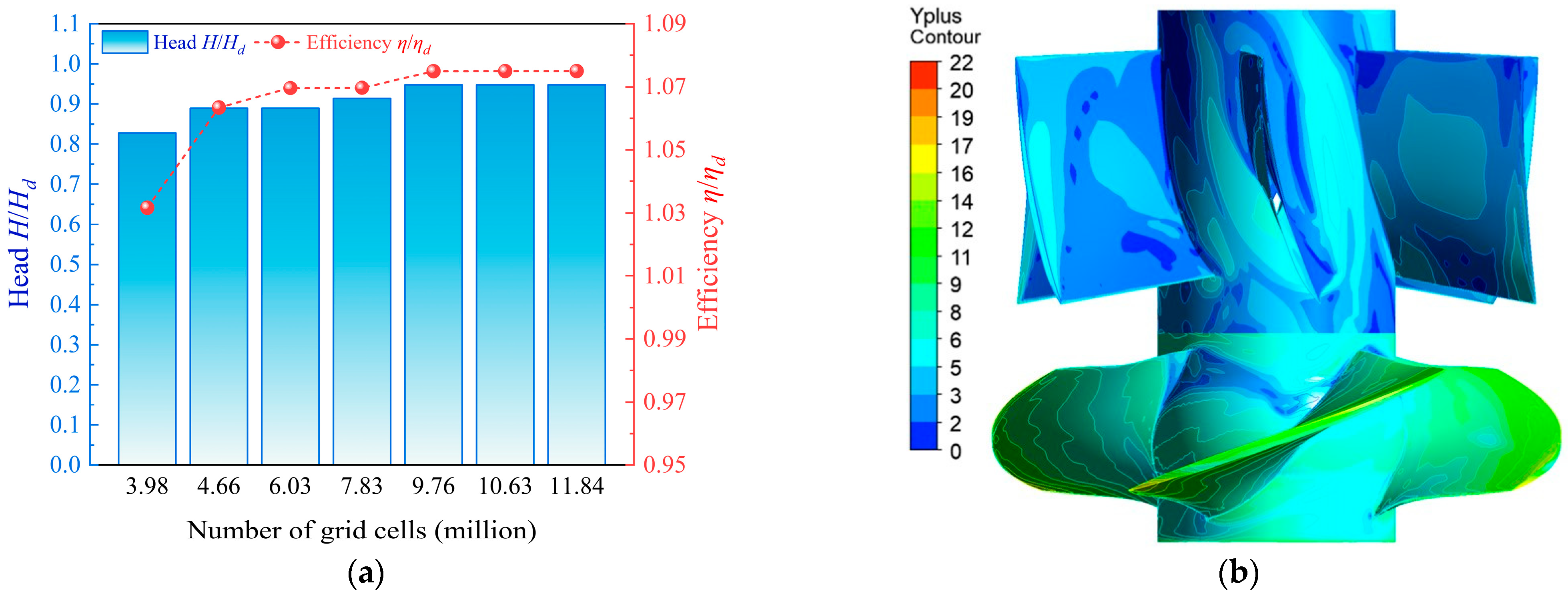
A grid independence verification was performed for seven mesh configurations of the axial flow pump device at the design flow rate Q_d, with the results shown in Figure 6a. In the figure, H_d represents the head corresponding to the design flow rate Q_d, and η_d represents the efficiency at the design flow rate Q_d. When the number of mesh cells exceeded 9.76 million, the simulated head and efficiency of the pump device remained virtually unchanged. To ensure the reliability of the numerical simulation and save computational time, this study was conducted using the mesh configuration with 10.63 million cells. The mesh quality was evaluated using the Determinant 3 × 3 × 3 metric in ANSYS ICEM CFD 19.0. For most cells, the determinant exceeds 0.5, indicating well-shaped cells with minimal distortion.

Figure 6. Mesh independence verification and Y-plus distribution: (a) Variation in head and efficiency with mesh density at the design flow rate; (b) Distribution of Y-plus values for the impeller and guide vane meshes.

According to the fundamental assumptions of viscous fluid mechanics, viscous effects between the fluid and the solid wall result in zero relative velocity at the wall. Y+ is a key parameter for evaluating the near-wall mesh quality and the applicability of the turbulence model [32]. Proper evaluation of Y+ ensures accurate simulation of the near-wall flow and prevents errors in pressure distribution or flow separation that could lead to incorrect cavitation predictions or non-convergent results. The calculation formula for Y-plus is given as:

$$y^{+}={\displaystyle \frac{\Delta y}{\nu }}\sqrt{{\displaystyle \frac{{\tau }_w}{\rho }}}$$

(8)

where $\Delta y$ is the first-layer grid height, m. $\rho$ is the fluid density, kg/m³, ${\tau }_w$ is the wall shear stress, Pa. $\nu$ is the kinematic viscosity, m²/s.

The y+ values for the impeller mesh and guide vane mesh are shown in Figure 6b.

4.3. Simulation Results Validation

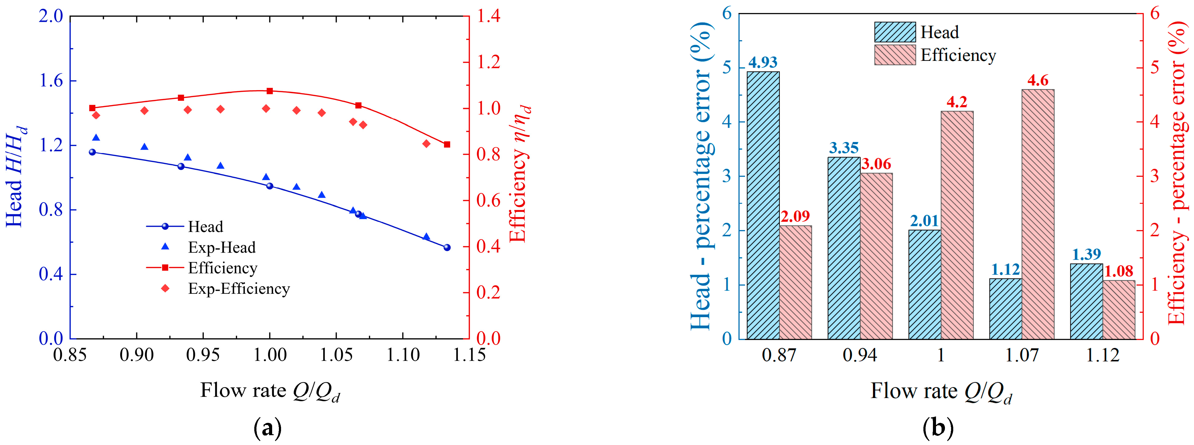
Figure 7a presents a comparison between the numerically simulated external characteristic curve and the experimentally measured external characteristic curve of the axial-flow pump device. Figure 7b shows the percentage error between the numerical simulation results and the experimental results of the external characteristics of the axial-flow pump device. As illustrated in Figure 7, the numerical simulation results of the external characteristics exhibit good agreement with the experimental data. The standard deviation of the head error is 0.031, and that of the efficiency error is 0.037. Under the five flow conditions examined, the percentage errors for both head and efficiency remain below 5%. These findings confirm that the numerical simulation provides sufficient accuracy to meet the requirements of this study.

Figure 7. Comparison of numerical and experimental external characteristics of the axial-flow pump device: (a) Performance curves obtained from numerical simulation and experiment; (b) Percentage error of head and efficiency between numerical and experimental results.

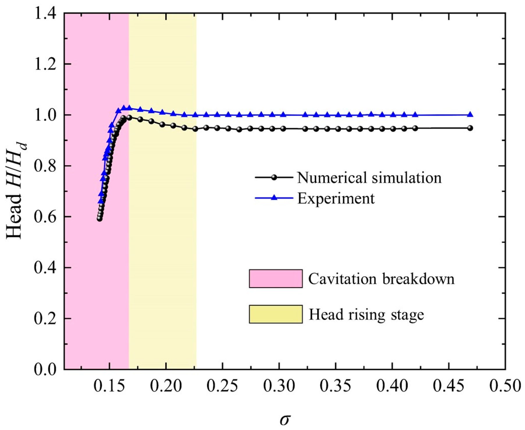
Figure 8 shows a comparison between the numerically simulated and experimentally measured cavitation performance curves of the axial-flow pump device under a flow rate of 1.0 Q_d.

Figure 8. Cavitation performance curve of the axial-flow pump at 1.0 Q_d.

As shown in Figure 8, the numerically simulated cavitation performance curve closely matches the experimental results. When the cavitation number σ is greater than 0.23, the head of the axial-flow pump remains stable. As σ decreases from 0.23 to 0.17, the head exhibits a slight increase: the numerically simulated head rises from 0.95 H_d to 0.98 H_d, and the experimentally measured head increases from 0.99 H_d to 1.03 H_d, as indicated by the yellow region in the figure. This phenomenon is attributed to the fact that moderate cavitation can improve the flow pattern in the impeller region. When σ further decreases below 0.17, the head drops sharply, indicating that the axial-flow pump enters the breakdown cavitation stage, denoted by the pink region in Figure 8. In this stage, the operational stability of the axial-flow pump is severely compromised.

5. Model Construction

5.1. Spider Wasp Optimization Algorithm

The Spider Wasp Optimization (SWO) algorithm [33] was proposed in 2023. This algorithm simulates the foraging, hunting, nesting, and mating behaviors of spider wasps, integrating both global exploration and local exploitation to provide an efficient and robust optimization strategy. Compared with other optimization algorithms such as Particle Swarm Optimization (PSO) and Genetic Algorithms (GA), SWO demonstrates superior convergence performance and search capability, making it well-suited for complex engineering data optimization and hyperparameter tuning in machine learning tasks.

The formula for initializing the population in the SWO algorithm is expressed as follows:

$$S{W}_i^t=L+r\cdot \left(H-L\right)$$

(9)

where $S{W}_i^t$ denotes the solution of the current time t, L and H represent the lower and upper bounds of the initial solution space, respectively, and r is a random vector with elements uniformly distributed in the range [0, 1].

During the exploration phase, spider wasps randomly adopt either a fixed-step random exploration mode or a variable-step local exploration mode. The calculation formula for the fixed-step random exploration mode is given as:

$$S{W}_i^{t+1}=S{W}_i^t+{\mu }_1\cdot \left(S{W}_a^t-S{W}_b^t\right)$$

(10)

where $S{W}_i^{t+1}$ represents the solution at the next iteration t + 1, ${\mu }_1$ is a control coefficient, and $S{W}_a^t$, $S{W}_b^t$ are two individuals randomly selected from the population.

$${\mu }_1=\left|r_n\right|\cdot r_1$$

(11)

where $r_1$ is a random number uniformly distributed in the interval [0, 1], and $r_n$ is a normally distributed random number.

The formula for the variable-step local exploration mode is:

$$S{W}_i^{t+1}=S{W}_c^t+{\mu }_2\cdot \left(L+r_2\cdot (H-L)\right)$$

(12)

where $S{W}_c^t$ is a randomly selected individual from the population, ${\mu }_2$ is a coefficient, and $r_2$ is a random number in [0, 1].

$${\mu }_2=B\cdot \cos \left(2\pi l\right)$$

(13)

$$B={\displaystyle \frac{1}{1+e^l}}$$

(14)

In the hunting phase, there are two possible states: successful capture and prey evasion. The corresponding formula is:

$$S{W}_i^{t+1}=S{W}_i^t+C\cdot \left|2\cdot r_5\cdot S{W}_a^t-S{W}_i^t\right|$$

(15)

where C is the distance factor determining the wasp’s speed. When C > 0.5, the spider wasp moves faster than the prey; when C < 0.5, it moves slower. $r_5$ is a random vector in [0, 1].

$$C=\left(2-2\cdot \left({\displaystyle \frac{f}{f_{\max }}}\right)\right)\cdot r_6$$

(16)

where f and f_max denote the current and maximum fitness values, respectively; $r_6$ is a random number in [0, 1].

As the prey escapes from the spider wasp, the distance between them increases. When this occurs, the hunting phase transitions to the exploration phase. The corresponding equation is as follows:

$$S{W}_i^{t+1}=v_c\cdot S{W}_i^t$$

(17)

where $v_c$ is a vector generated from a normal distribution within the range [−k, k], $k=1-\left({\displaystyle \frac{f}{f_{\max }}}\right)$.

During the nesting phase, spider wasps exhibit two behavioral strategies: 1. Dragging the spider to the most suitable location, formulated as:

$$S{W}_i^{t+1}=S{W}^{*}+\cos \left(2\pi l\right)\cdot \left(S{W}^{*}-S{W}_i^t\right)$$

(18)

where $S{W}^{\ast }$ is the current best solution.

Randomly selecting a region of the female spider wasp:

$$S{W}_i^{t+1}=S{W}_a^t+r_3\cdot \left|\gamma \right|\cdot \left(S{W}_a^t-S{W}_i^t\right)+\left(1-r_3\right)\cdot U\cdot \left(S{W}_b^t-S{W}_c^t\right)$$

(19)

where $r_3$ is a random number in [0, 1]; $\gamma$ is a value generated according to the Lévy flight model; U is a binary vector composed of random 0 s or 1 s; and $S{W}_c^t$ is a randomly selected individual from the population.

The formula for generating new individuals through mating is:

$$S{W}_i^{t+1}=Crossover\left(S{W}_i^t,S{W}_m^t,C_R\right)$$

(20)

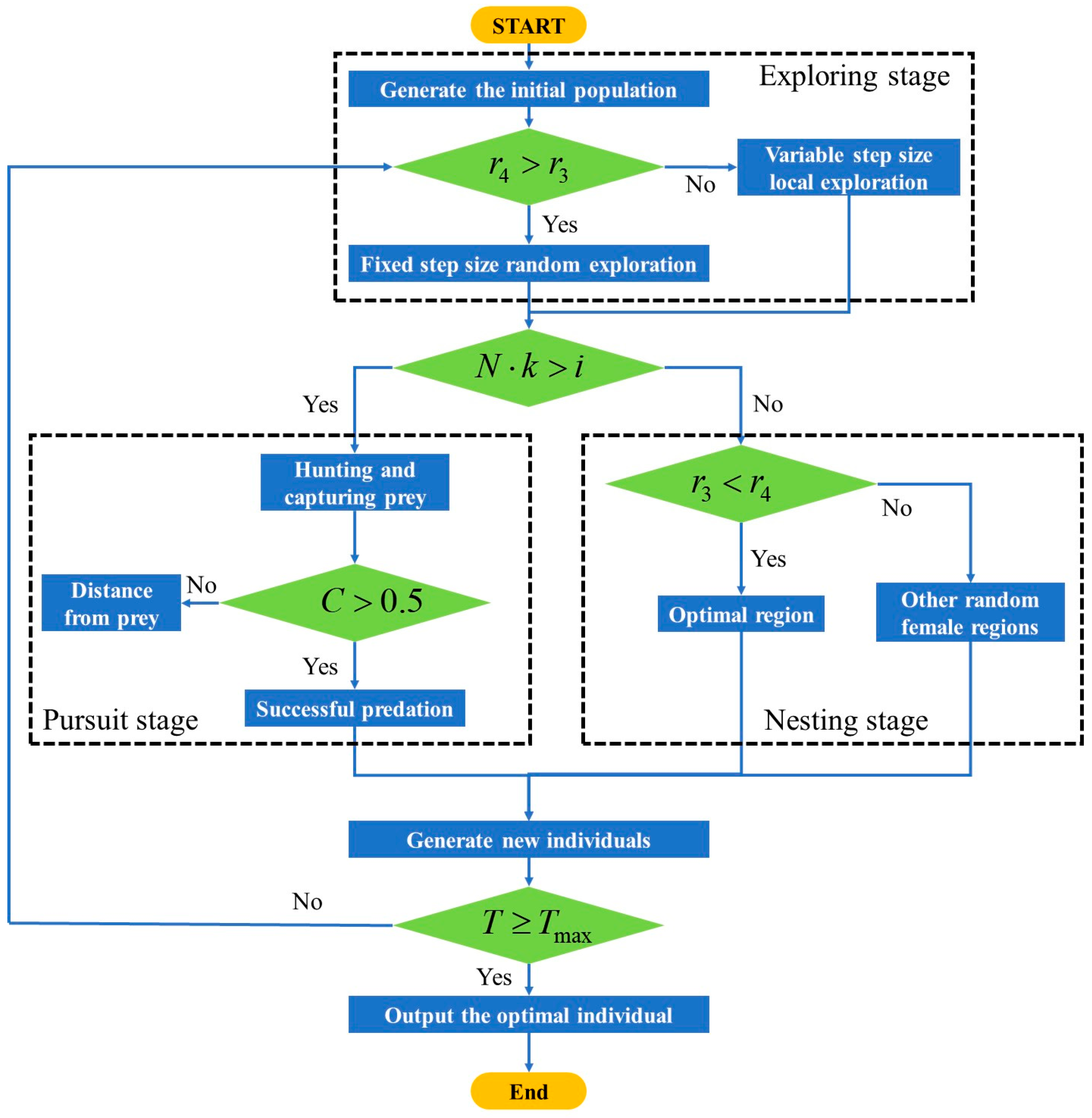
where Crossover() is the uniform crossover operator, $S{W}_m^t$ represents the male spider wasp vector, and $C_R$ is the crossover probability. The basic procedure of the SWO algorithm is shown in Figure 9, where $r_4$ denotes a uniformly distributed random number in [0, 1], N is the initial population, T is the current iteration number, and T_max is the maximum number of iterations.

Figure 9. SWO algorithm flowchart.

5.2. BiLSTM Model Optimization

This study combines the Spider Web Optimization (SWO) algorithm with the Bidirectional Long Short-Term Memory (BiLSTM) network to establish the SWO-BiLSTM model. BiLSTM is a specialized type of recurrent neural network consisting of two LSTM layers—one processes the forward sequence (from start to end), while the other processes the backward sequence (from end to start) [34]. The forward LSTM handles the sequence in a left-to-right information flow. Each unit of the forward LSTM receives the current input $x_t$, as well as the hidden state $h_{t-1}^f$ and cell state $c_{t-1}^f$ from the previous time step, and then updates its state to the current time step. The BiLSTM architecture is shown in Figure 10.

Figure 10. BiLSTM schematic diagram.

(1)

The input gate $i_t^f$ controls how much of the current input is received, and its expression is given by:

$$i_t^f=S\cdot \left(W_{xi}^f{x}_t+W_{hi}^f{h}_{t-1}^f+b_i^f\right)$$

(21)

where $i_t^f$ denotes the input gate value at time step t in the forward direction; $S$ represents the sigmoid function, which maps input values to the range [0, 1]; $W_{xi}^f$ is the weight matrix from the input $x_t$ to the input gate; $W_{hi}^f$ is the weight matrix from the previous hidden state $h_{t-1}^f$ to the input gate; $b_i^f$ is the bias term for the input gate i.

(2)

The forget gate f determines how much of the previous memory is retained, expressed as:

$$f_t^f=S\cdot \left(W_{xf}^f{x}_t+W_{hf}^f{h}_{t-1}^f+b_f^f\right)$$

(22)

where $f_t^f$ is the forget gate value at time step t; $W_{xf}^f$ and $W_{hf}^f$ are the weight matrices from the input and the previous hidden state to the forget gate, respectively; $b_f^f$ is the bias term for the forget gate.

(3)

The cell state c is updated based on the input and forget gates as follows:

$$c_t^f=f_t^f\cdot c_{t-1}^f+i_t^f\cdot \tanh \left(W_{xc}^f{x}_t+W_{hc}^f{h}_{t-1}^f+b_c^f\right)$$

(23)

where $c_t^f$ is the cell state at time t; $\tanh$ is the activation function used to map the input to the range of [−1, 1]; $W_{xc}^f$ and $W_{hc}^f$ are the weight matrices from the input and the previous hidden state to the cell state, respectively; $b_c^f$ is the bias term for the cell state.

(4)

The output gate $o_t^f$ determines how much of the current cell state is output to the hidden state, expressed as:

$$o_t^f=S\cdot \left(W_{xo}^f{x}_t+W_{ho}^f{h}_{t-1}^f+b_o^f\right)$$

(24)

where $o_t^f$ is the output gate value at time t; $W_{xo}^f$ and $W_{ho}^f$ are the weight matrices from the input and hidden state to the output gate; $b_o^f$ is the bias term for the output gate.

(5)

The hidden state $h_t^f$ is calculated based on the output gate and the current cell state:

$$h_t^f=o_t^f\cdot \tanh \left(c_t^f\right)$$

(25)

where $o_t^f$ is the output gate value; $c_t^f$ is the cell state at time t.

(6)

The mathematical formulation of the backward LSTM is similar to the forward LSTM, but the time direction is reversed. In a BiLSTM, at each time step t, the forward and backward hidden states are concatenated to form a new hidden layer output:

$$h_t=\left[h_t^f;h_t^b\right]$$

(26)

where $h_t$ denotes the bidirectional LSTM hidden state at time step t; $h_t^f$ and $h_t^b$ are the forward and backward LSTM hidden states, respectively.

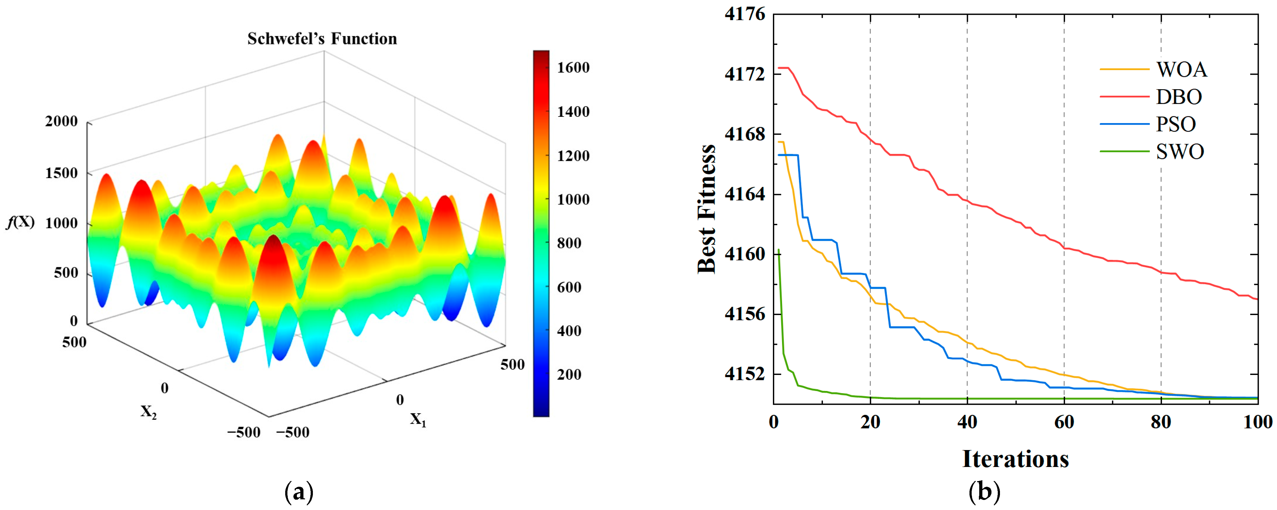
Hyperparameters significantly influence the prediction accuracy of neural network models. However, no universally applicable method exists for setting hyperparameters, which are typically tuned through repeated trial and error. To improve both prediction accuracy and efficiency, this study selects the number of training epochs, learning rate, number of hidden layer neurons, and regularization coefficient as decision variables to be optimized. The mean squared error (MSE) is used as the fitness function. To evaluate optimization performance, Schwefel’s Function is adopted as the benchmark function:

$$f\left(x\right)=418.9829\times n-{\displaystyle \sum _{i=1}^n{x}_i}\sin \left(\sqrt{\left|x_i\right|}\right)$$

(27)

Schwefel’s Function is a multimodal function with many local minima, making it suitable for testing the capability of global optimization algorithms on complex problems [35]. Figure 11a illustrates the two-dimensional response surface of Schwefel’s Function with two decision variables, while Figure 11b presents the convergence curves of various optimization algorithms under the Schwefel test, with the problem dimension set to 50 and the population size of all algorithms fixed at 100.

Figure 11. Convergence behavior of the optimization algorithms: (a) Two-dimensional response surface of the Schwefel’s Function; (b) Convergence curves obtained under the Schwefel test (dimension = 50; population size = 100).

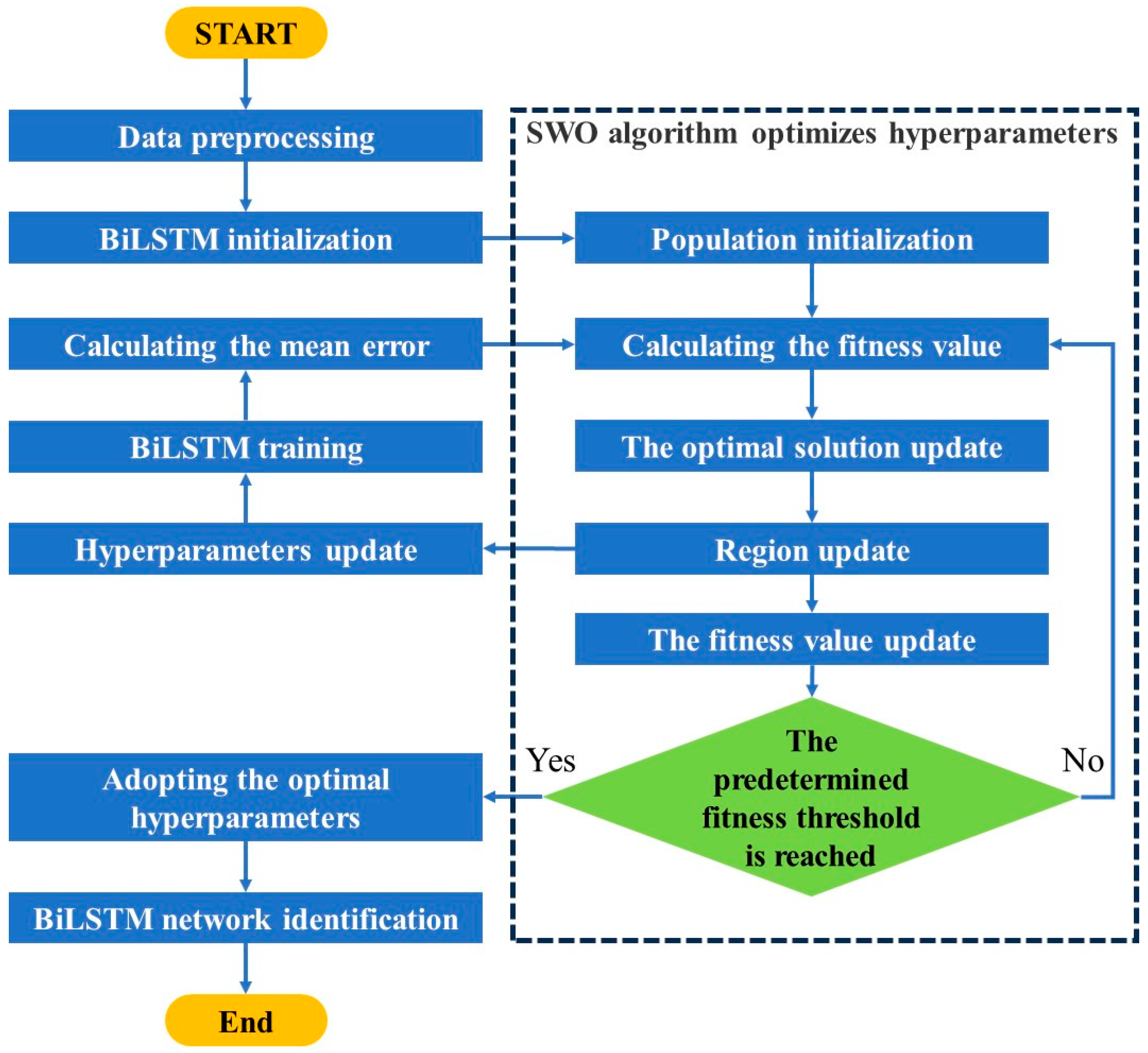
As shown in Figure 11b, the Spider Wasp Optimization (SWO) algorithm demonstrates both fast convergence and high precision, indicating superior optimization performance compared to other algorithms. Therefore, SWO is employed to optimize the BiLSTM model, forming the SWO-BiLSTM optimized prediction framework. The SWO-BiLSTM model identification process is illustrated in Figure 12 and consists of the following steps:

Figure 12. Identification process of the SWO-BiLSTM model.

Step 1: Based on the CFD unsteady simulation results under various cavitation numbers, preprocess the simulated pressure fluctuation signals and extract signal features to serve as the input for the BiLSTM model.

Step 2: Initialize the spider wasp population, define the hyperparameter search range, evaluate fitness using average error, and record the optimal solution.

Step 3: Update the position of each spider wasp. Use the updated position as the new set of BiLSTM hyperparameters, train the neural network, compute training error, and seek the optimal solution.

Step 4: Check whether the fitness meets the specified condition. If satisfied, output the corresponding hyperparameters as the final configuration for the BiLSTM model; otherwise, return to Step 3 for further optimization.

5.3. Model Input Optimization

Due to the influence of cavitation, the pressure fluctuation signals within the axial flow pump exhibit nonlinear characteristics. Traditional methods, such as the Fourier and Wavelet Transforms, have limitations when handling such signals. Variational Mode Decomposition (VMD) does not rely on any predefined basis functions, but instead adaptively determines the frequency band of each mode through optimization algorithms [36]. This adaptive feature allows VMD to better capture the complex frequency variations within the signal, especially when multiple frequency components are present, providing higher decomposition accuracy. During the decomposition process, VMD effectively extracts the main modes of the signal while suppressing noise. By decomposing the pressure fluctuation signal, VMD enables the separation of noise components from the true signal, thereby facilitating the extraction of meaningful features in subsequent analysis.

Assuming a signal $f\left(t\right)$ is decomposed by the Variational Mode Decomposition (VMD) algorithm into k Intrinsic Mode Functions (IMFs), the VMD process can be expressed as:

$$\left\{\begin{array}{c}\underset{\left\{u_k\right\},\left\{w_k\right\}}{\min }\left\{{\displaystyle \sum _k{\left|{\partial }_t\left[\left(\delta \left(t\right)+\frac{j}{\pi t}\right)\ast u_k\left(t\right)\right]e^{-j{\omega }_{k}t}\right|}_2^2}\right\}\hfill \\ \mathrm{s}.\mathrm{t}.{\displaystyle \sum _k{u}_k\left(t\right)=f\left(t\right)}\hfill \end{array}\right.$$

(28)

where $\delta \left(t\right)$ denotes the Dirac delta function, $u_k\left(t\right)$ represents the k-th IMF, ${\omega }_k\left(t\right)$ is the center frequency of the k-th IMF, and j denotes the imaginary unit.

Sample Entropy (SampEn) is a statistical metric used to quantify the complexity and unpredictability of time series data [37]. It is particularly effective in identifying the degree of regularity or irregularity present in a signal. A higher SampEn value indicates greater irregularity or complexity within the sequence, while a lower value suggests stronger regularity. SampEn addresses the bias inherent in Approximate Entropy (ApEn) and offers improved robustness and accuracy, making it widely applicable in signal processing. The definition of Sample Entropy proceeds as follows:

Given a time series of length N, denoted as $\left\{x_1,x_2,\cdot \cdot \cdot ,x_N\right\}$, construct a sequence of embedded vectors of dimension m, each of the form $X_m\left(i\right)=\left\{x_i,x_{i+1},\cdot \cdot \cdot ,x_{i+m-1}\right\}$. SampEn is computed by evaluating the similarity between different patterns in the sequence.

For each subsequence $X_m\left(i\right)$, the Chebyshev distance is used to calculate its distance D from other subsequences $X_m\left(j\right)$. The number of subsequences satisfying $D\le r$ is counted as $A_i$, and the average value is calculated as $A_m\left(r\right)$. For m + 1 dimensional subsequences, the corresponding average is denoted as $A_{m+1}\left(r\right)$. The sample entropy is then defined as:

$$\mathrm{SampEn}\left(m,r\right)=-\ln \left({\displaystyle \frac{A_m\left(r\right)}{A_{m+1}\left(r\right)}}\right)$$

(29)

where $A_m\left(r\right)$ represents the similarity probability of embedded vector pairs with a length of m, and $A_{m+1}\left(r\right)$ represents the similarity probability of embedded vector pairs with a length of m + 1.

In this study, the input of the model consists of a feature matrix extracted from the pressure fluctuation signal. The feature extraction and input optimization steps are as follows:

Step 1: Decompose the pressure fluctuation signal using the VMD algorithm to obtain the Intrinsic Mode Functions (IMFs) of the original signal.

Step 2: Extract the dominant frequency components and corresponding amplitudes from the IMFs.

Step 3: Compute the Sample Entropy of each IMF. Combine these entropy values with the dominant frequencies and amplitudes obtained in Step 2 to form the input feature matrix.

The input matrix is shown in Equation (30). ${\mathrm{SE}}_j$ represents the sample entropy of the j-th IMF, and ${\mathrm{F}}_{jk}$ denotes the k-th dominant frequency of the j-th IMF, where k = 1 indicates the primary frequency, k = 2 the secondary frequency, and k = 3 the harmonic frequency. ${\mathrm{A}}_{jk}$ represents the amplitude corresponding to the k-th dominant frequency of the j-th IMF.

$$\left[\begin{array}{ccccccc}{\mathrm{SE}}_1& {\mathrm{F}}_{11}& {\mathrm{A}}_{11}& {\mathrm{F}}_{12}& {\mathrm{A}}_{12}& {\mathrm{F}}_{13}& {\mathrm{A}}_{13}\\ {\mathrm{SE}}_2& {\mathrm{F}}_{21}& {\mathrm{A}}_{21}& {\mathrm{F}}_{22}& {\mathrm{A}}_{22}& {\mathrm{F}}_{23}& {\mathrm{A}}_{23}\\ {\mathrm{SE}}_3& {\mathrm{F}}_{31}& {\mathrm{A}}_{31}& {\mathrm{F}}_{32}& {\mathrm{A}}_{32}& {\mathrm{F}}_{33}& {\mathrm{A}}_{33}\\ {\mathrm{SE}}_4& {\mathrm{F}}_{41}& {\mathrm{A}}_{41}& {\mathrm{F}}_{42}& {\mathrm{A}}_{42}& {\mathrm{F}}_{43}& {\mathrm{A}}_{43}\end{array}\right]$$

(30)

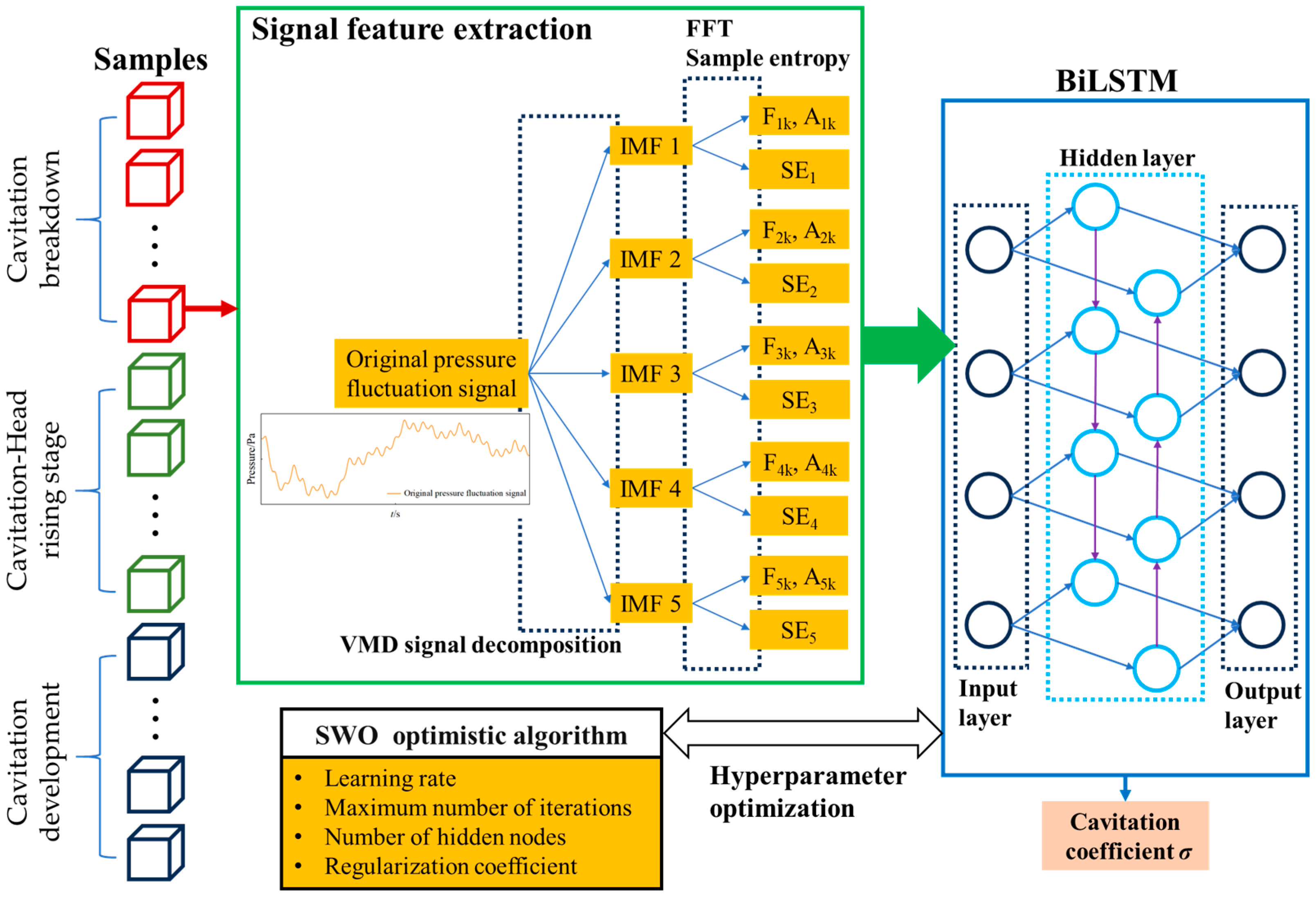
The overall structure of the VMD-SWO-BiLSTM model proposed in this research for cavitation coefficient identification in an axial flow pump is shown in Figure 13.

Figure 13. The overall structure of the VMD-SWO-BiLSTM model.

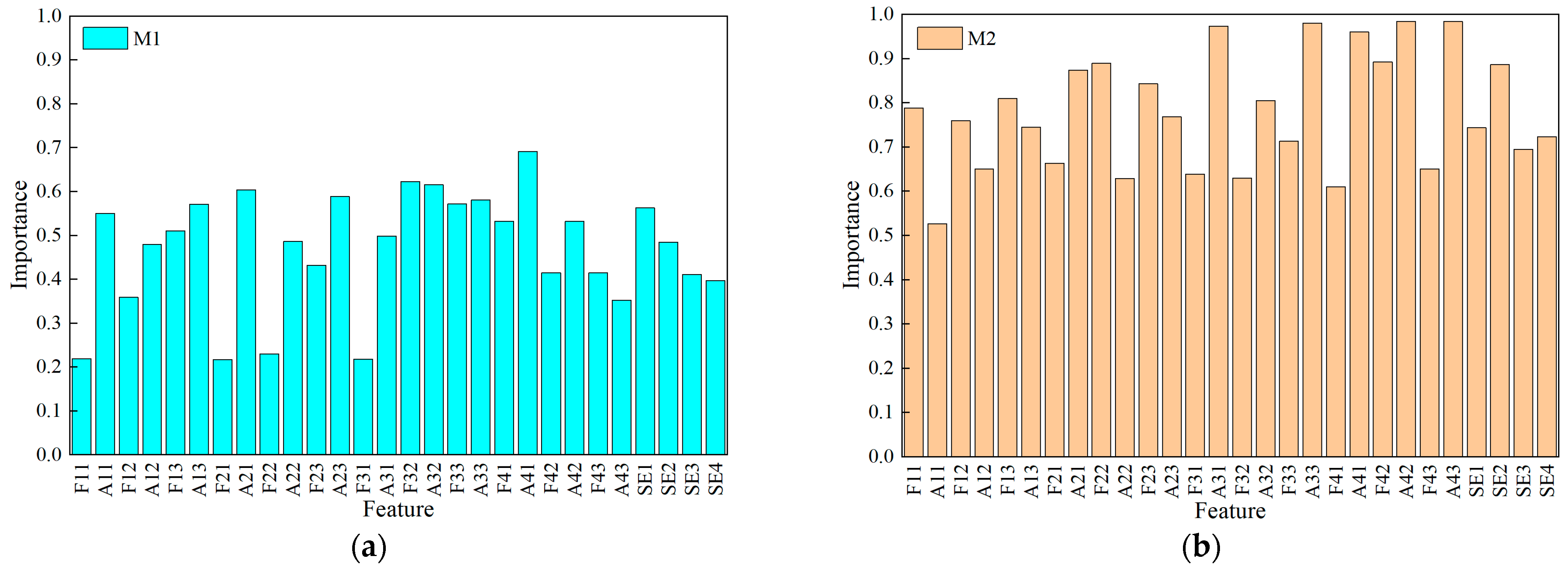
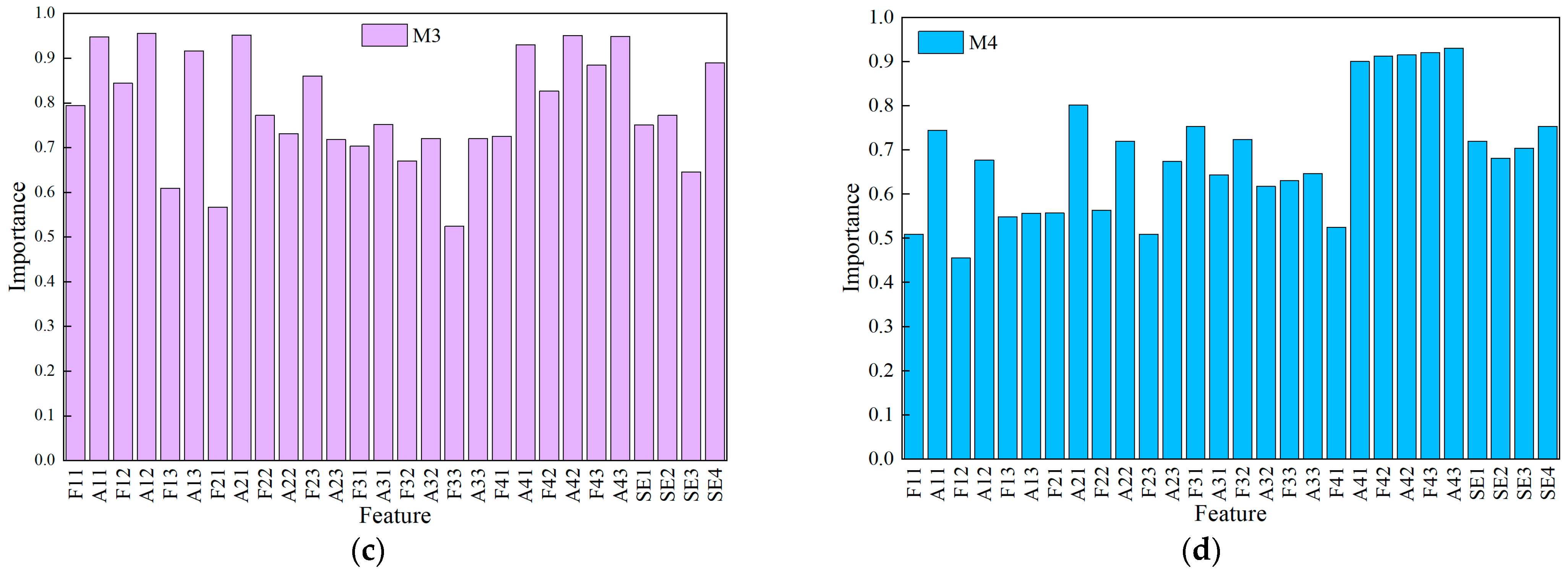
To quantify the contribution of each input feature, a random forest regression model with permutation importance was employed. Permutation importance evaluates feature relevance by randomly permuting a single feature and measuring the resulting increase in prediction error, which makes it well-suited for capturing nonlinear relationships and provides an interpretable measure of feature contribution. The importance of the pressure fluctuation features for all the numerical simulation samples is shown in Figure 14. A feature importance value closer to 1 indicates a more influential feature.

Figure 14. Importance analysis of pressure fluctuation features based on Random Forest permutation importance: (a) Measurement point M1; (b) Measurement point M2; (c) Measurement point M3; (d) Measurement point M4.

According to Figure 14, the pressure fluctuation features at the M1 measurement point exhibit relatively low importance. All feature importance scores at the M2 and M3 measurement points are higher than 0.5, while at the M4 measurement point, the importance score of F12 is lower than 0.5. Therefore, in this study, the pressure fluctuation features from the M2 and M3 measurement points were selected as the model inputs.

5.4. Optimization Process Analysis

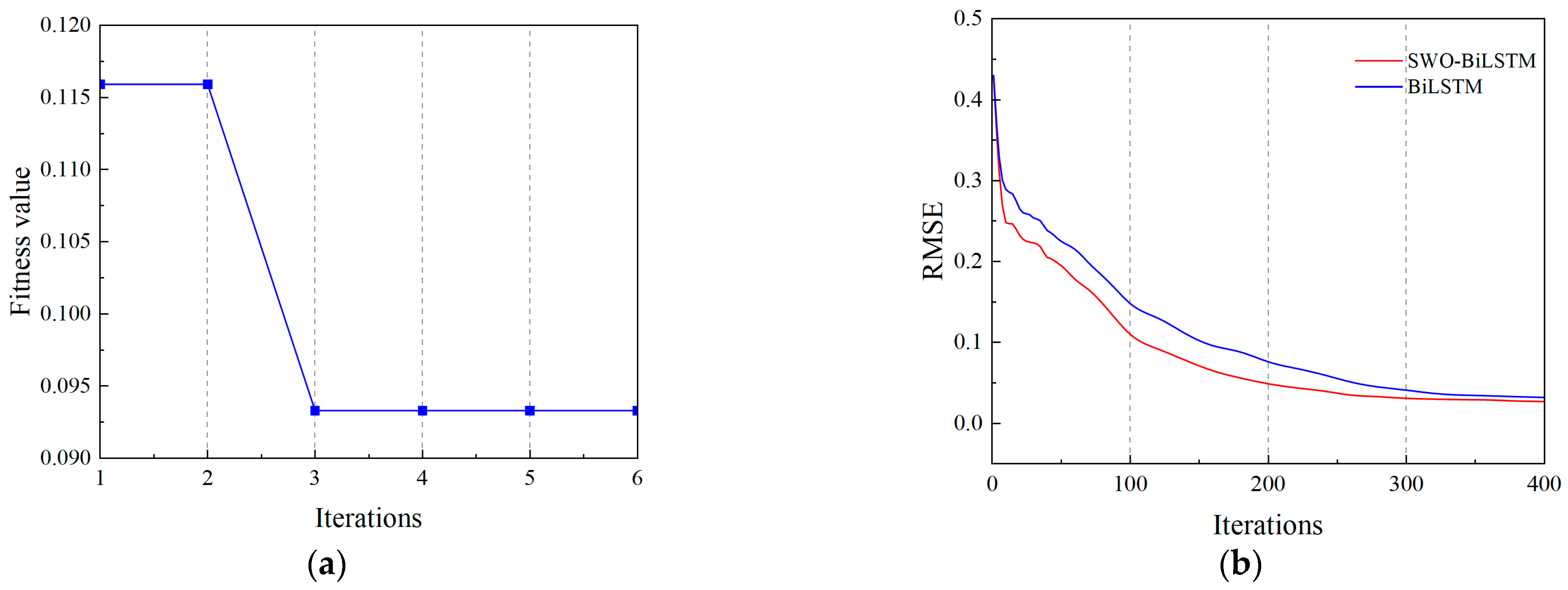
To verify the feasibility of using SWO to determine the hyperparameters of the SWO-BiLSTM model, the search ranges for the number of neurons in the BiLSTM layer, learning rate, regularization parameter, and maximum number of training iterations were set to [10, 80], [0.001, 0.01], [0.0001, 0.001], and [100, 500], respectively. After iterative convergence, the optimized hyperparameters obtained were 68 neurons in the BiLSTM layer, a learning rate of 0.0047, a regularization parameter of $1.47\times {10}^{-4}$, and 340 maximum iterations. To reduce the risk of overfitting, dropout regularization was applied to the BiLSTM layers, randomly deactivating 20% of neurons during training. Figure 15a shows the evolution curve of the best fitness obtained through iterative SWO updates, and Figure 15b presents the model training curve.

Figure 15. Optimization process analysis: (a) Evolution of the best fitness value during the SWO iterations; (b) Training convergence curves.

As shown in Figure 15a, the fitness value converges after the third iteration, and the optimal fitness solution is finally obtained. According to Figure 15b, the BiLSTM model optimized by SWO converges faster and achieves a relatively lower Root Mean Square Error (RMSE).

6. Cavitation Coefficient Identification

6.1. Model Training and Testing

When cavitation occurs in the axial flow pump, its internal flow characteristics and pressure distribution are significantly affected, which in turn alters the frequency components and amplitudes of the pressure fluctuation signals in certain regions of the pump device. In this study, the unsteady internal flow of the axial flow pump under different cavitation coefficients was calculated. Considering the head variation in the cavitation performance curve transition region and the significant drop in head during the cavitation breakdown stage, as well as the disturbed internal flow and pronounced pressure fluctuation features, this study focuses on a denser sample distribution during these two stages. Thus, during the breakdown cavitation stage ($0.1422\le \sigma \le 0.1675$), 52 samples were obtained; during the head rise stage ($0.1698\le \sigma \le 0.2258$), 21 samples were calculated; and during the cavitation development stage ($0.2287\le \sigma \le 0.4688$), 60 samples were obtained. In total, 133 samples were collected, each corresponding to a cavitation coefficient σ, as shown in Table 2.

Table 2. Sample–cavitation coefficient correspondence table.

Cavitation Stage	Sample Number	Cavitation Coefficient σ
Cavitation breakdown	1	0.1422
	2	0.1424
	3	0.1425
	…	…
	52	0.1675
Head rising stage	53	0.1698
	54	0.1711
	…	…
	73	0.2258
Cavitation development	74	0.2287
	75	0.2313
	…	…
	133	0.4688

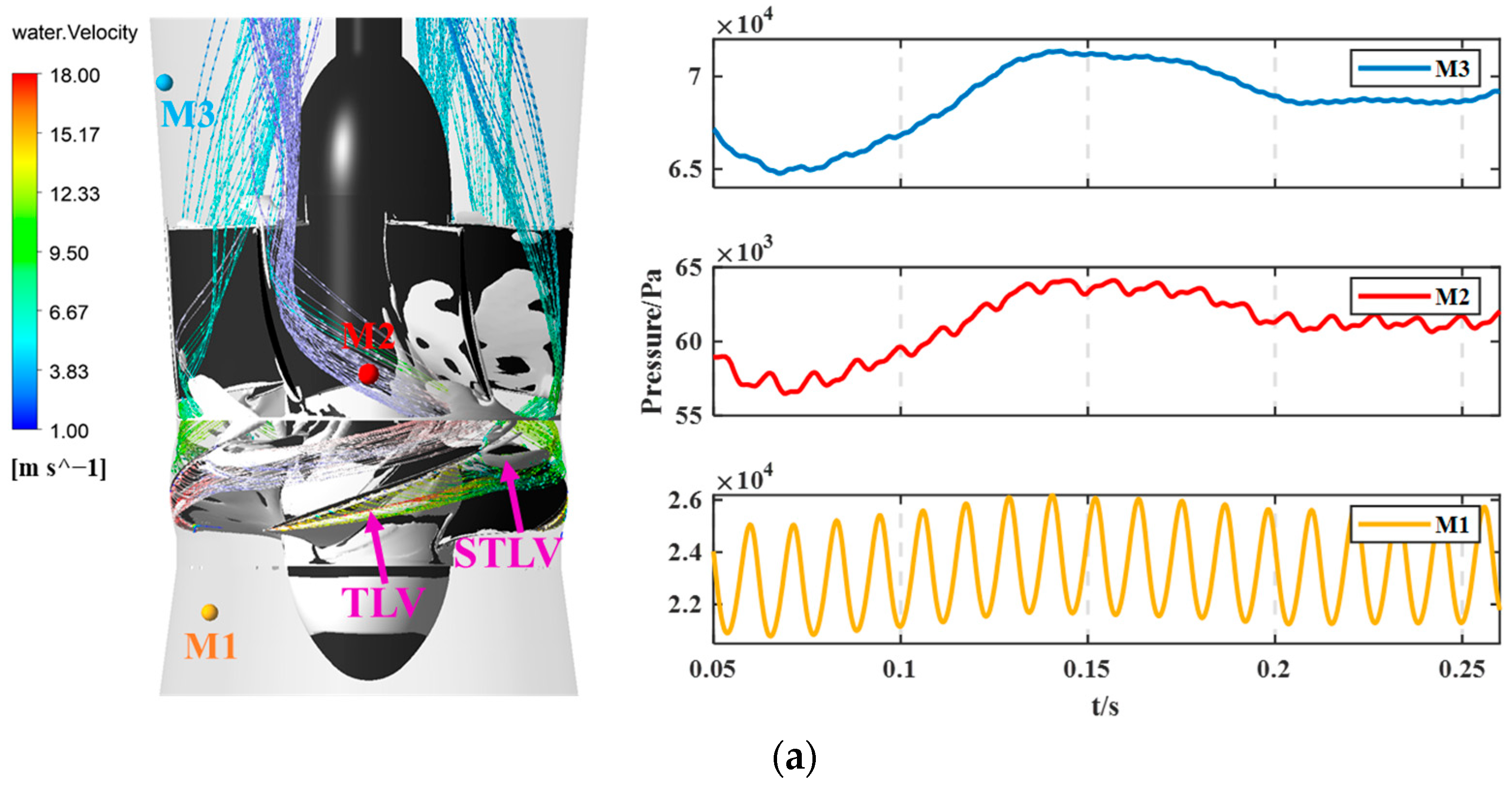
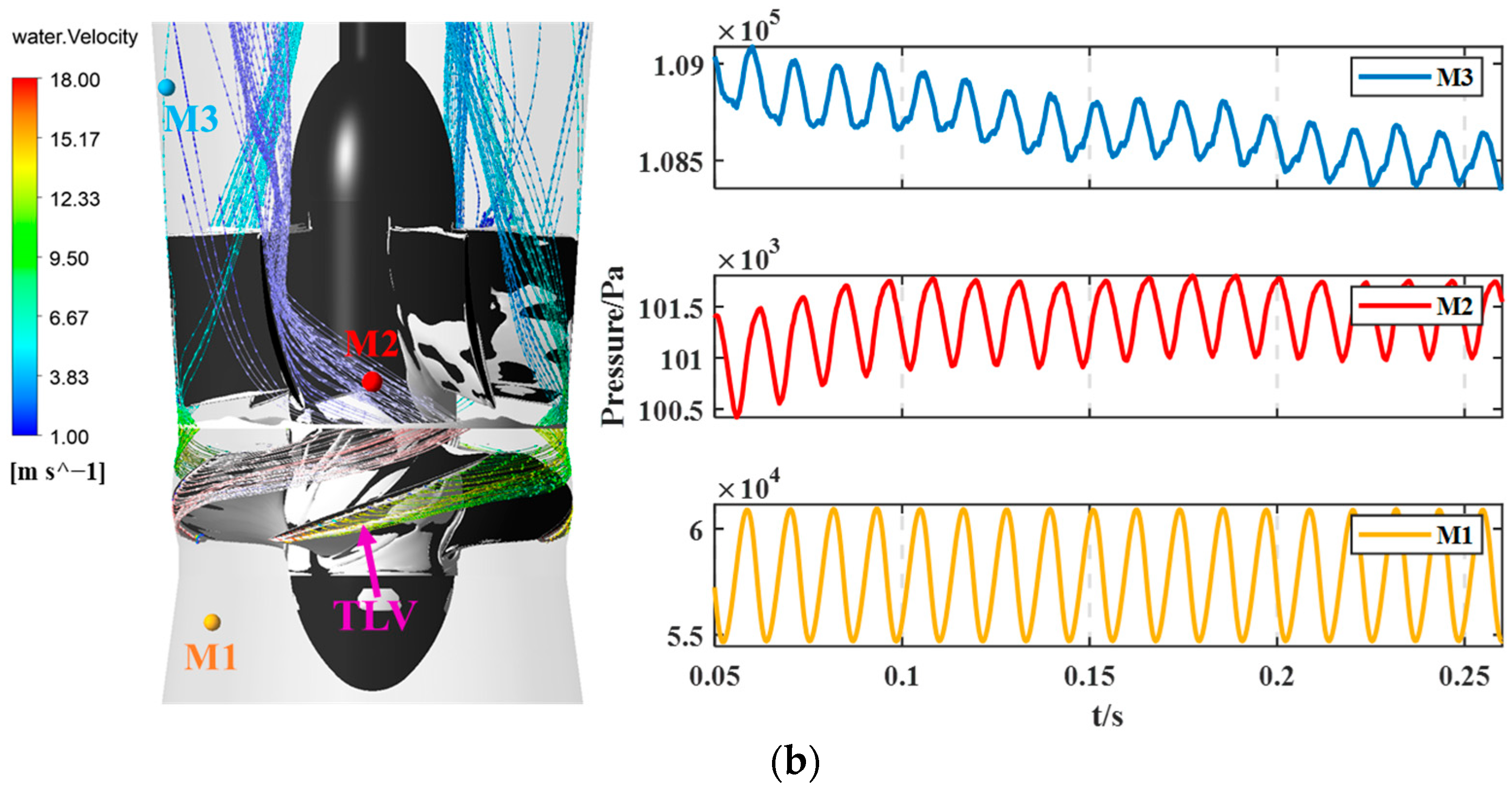
Figure 16 shows the numerical simulation results for the Omega vortex identification in the internal flow of the axial flow pump, as well as the pressure fluctuation time-domain data at three different measurement points (M1, M2, M3) for σ values of 0.1578 and 0.3231.

Figure 16. Numerical results of internal flow patterns and time-domain pressure fluctuations inside the axial flow pump at measurement points M1, M2, and M3 under two cavitation conditions. (a) Cavitation condition: $\sigma =0.1578$. (b) Cavitation condition: $\sigma =0.3231$.

In Figure 16a, a leakage vortex appears near the blade tip, and a separation leakage vortex is observed near the trailing edge of the blade tip. In Figure 16b, only a leakage vortex near the blade tip is observed. This is because, at σ = 0.1578, the axial flow pump operates in the breakdown cavitation stage, where large cavitation bubbles attach to the suction side of the blades, causing a significant pressure difference and flow separation, leading to the formation of the separation vortex at the blade tip. The separation vortex at the blade tip affects the streamlines in the blade tip region, altering the flow conditions at the M2 and M3 measurement points, significantly impacting the pressure fluctuation signals at these points, as shown in the pressure fluctuation time-domain graphs. The above analysis indicates that cavitation significantly alters the frequency components and amplitudes of the pressure fluctuation signals at different locations inside the axial flow pump. The measurement points used in this study are effective in capturing the impact of cavitation on pressure fluctuation signals.

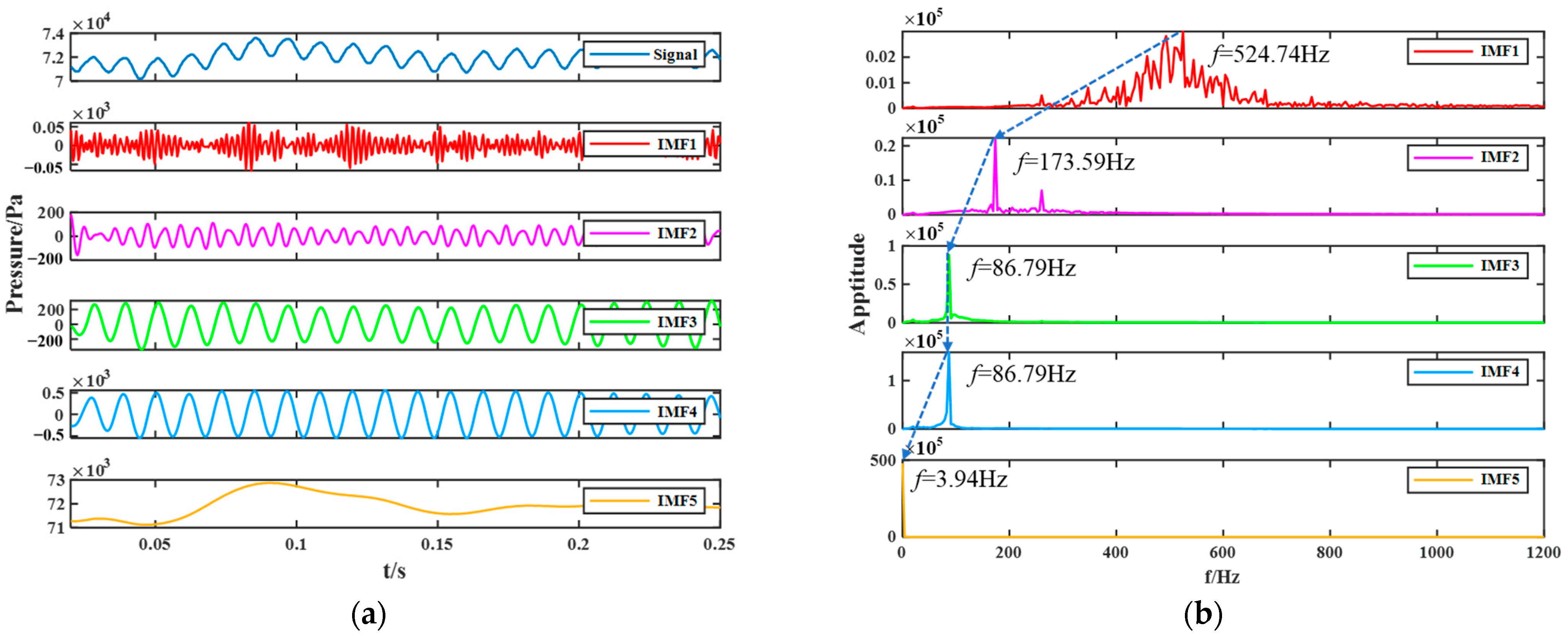
To quantify the effect of cavitation on the pressure fluctuation signal, the characteristics of the pressure fluctuation signals were extracted as inputs for the model. This study employed Variational Mode Decomposition (VMD) to decompose the simulated pressure fluctuation signals into multiple intrinsic mode functions (IMFs). Each IMF corresponds to different frequency bands, reflecting the pressure variation in different regions of the pump’s flow field, and capturing the effect of cavitation on the pressure fluctuation. First, the IMFs of the pressure fluctuation signals obtained by VMD were subjected to Fast Fourier Transform (FFT), and the FFT results were analyzed. The FFT results extract the frequency-domain features of the IMFs, which reflect the frequency components and corresponding amplitudes related to cavitation in the axial flow pump. Using the signal data monitored at point M2 as an example, under the cavitation condition of σ = 0.1773, the numerically simulated pressure fluctuation signal at M2 and its intrinsic mode functions (IMFs) obtained from VMD are shown in Figure 17a. Figure 17b presents the frequency-domain distributions of these five IMFs after applying FFT.

Figure 17. Signal decomposition at M2 monitoring point ($\sigma =0.1773$): (a) Original pressure fluctuation signal and its IMFs obtained from VMD; (b) The frequency-domain distribution of the IMFs.

As observed in Figure 17, the main frequency of IMF1 appears in the high-frequency region at 524.74 Hz. IMF2 has a main frequency of 173.59 Hz, IMF3 has a main frequency of 86.79 Hz (blade passing frequency), and IMF4 corresponds to the blade frequency at 86.79 Hz. IMF5 has a main frequency in the low-frequency range with an excessively high amplitude, indicating that IMF5 is a noise disturbance and lacks reference values.

Table 3 provides detailed information on the sample entropy, major frequency components, and corresponding amplitudes of the IMFs for the numerical simulation pressure fluctuation signal at M2 for σ = 0.4. Here, SE represents the sample entropy, F₁ denotes the primary frequency, A₁ represents the amplitude of the primary frequency, F₂ is the secondary frequency, A₂ is the amplitude of the secondary frequency, F₃ is the harmonic frequency, and A₃ is the amplitude of the harmonic frequency.

Table 3. Characteristic values of signals at M2 monitoring point (σ = 0.4).

Eigenvalue	IMF1	IMF2	IMF3	IMF4
SE	$0.20$	$0.27$	$0.13$	$0.12$
F1 (Hz)	$260.39$	$173.59$	$86.79$	$86.79$
A1	$2.99\times {10}^3$	$2.23\times {10}^4$	$8.81\times {10}^4$	$1.59\times {10}^5$
F2 (Hz)	$493.17$	$260.39$	$82.85$	$82.85$
A2	$2.82\times {10}^3$	$7.06\times {10}^3$	$1.51\times {10}^4$	$3.51\times {10}^4$
F3 (Hz)	$489.23$	$165.71$	$98.63$	$78.91$
A3	$2.59\times {10}^3$	$2.97\times {10}^3$	$1.03\times {10}^4$	$1.92\times {10}^4$

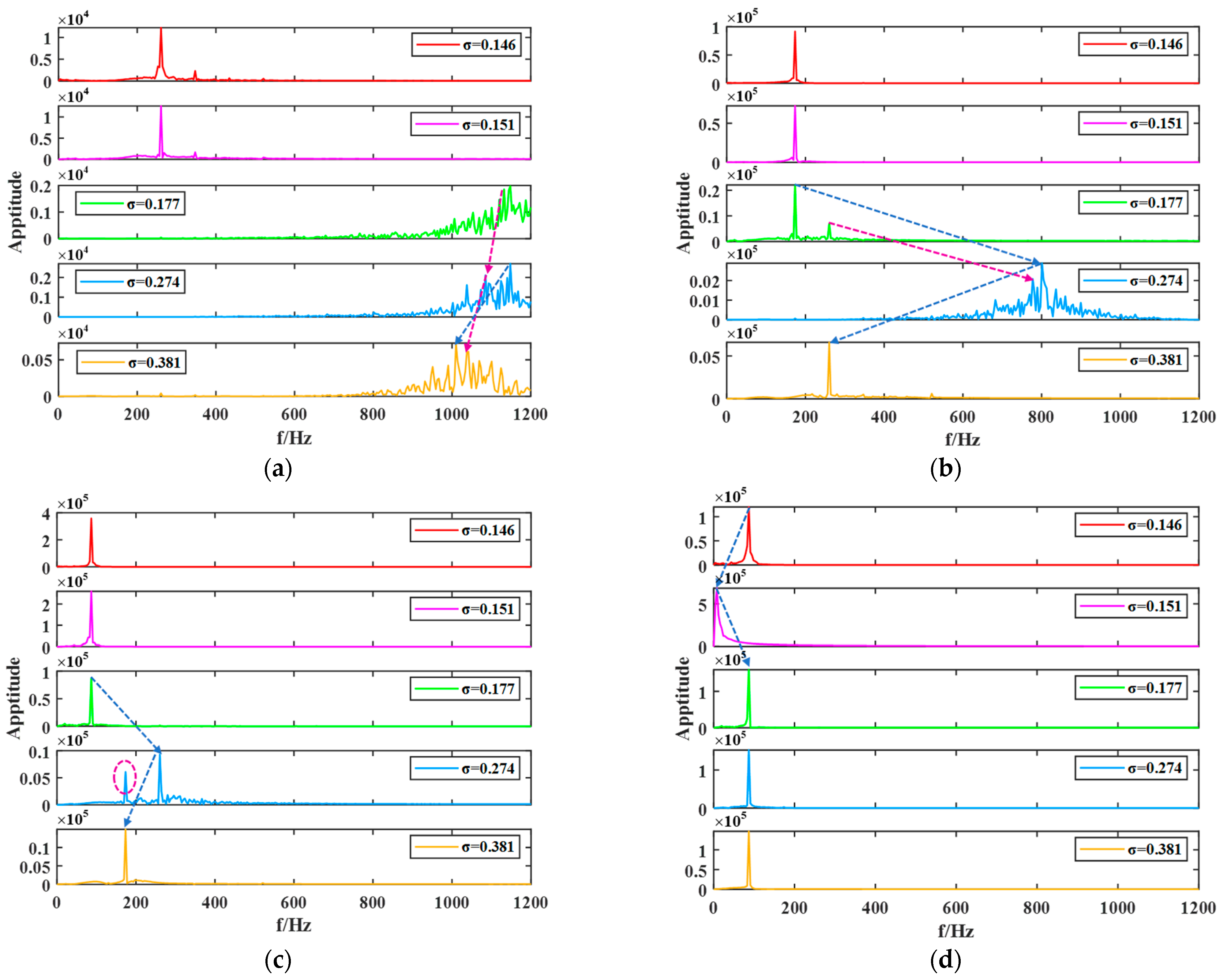
To analyze the effect of the internal flow field on the IMFs of the axial-flow pump under different cavitation numbers σ, five signal decomposition results were selected from the sample set at monitoring point M2 for frequency-domain comparison. These five samples represent five different cavitation conditions, as shown in Figure 18.

Figure 18. Frequency-domain comparison of IMFs at monitoring point M2 under five cavitation conditions: (a) Measurement point M1; (b) Measurement point M2; (c) Measurement point M3; (d) Measurement point M4.

As observed in Figure 18, the main frequency components and amplitudes of IMF1, IMF2, IMF3, and IMF4 at M2 vary to some extent under different σ values. At the same time, there are instances where the main frequency of the IMFs does not change with the cavitation degree, as seen in Figure 18a, where the main frequency of IMF1 is the same for σ values of 0.146 and 0.151, with the difference being in the amplitude of the main frequency. Therefore, it is necessary to perform a detailed analysis of the frequency and amplitude distributions of the IMFs across all samples.

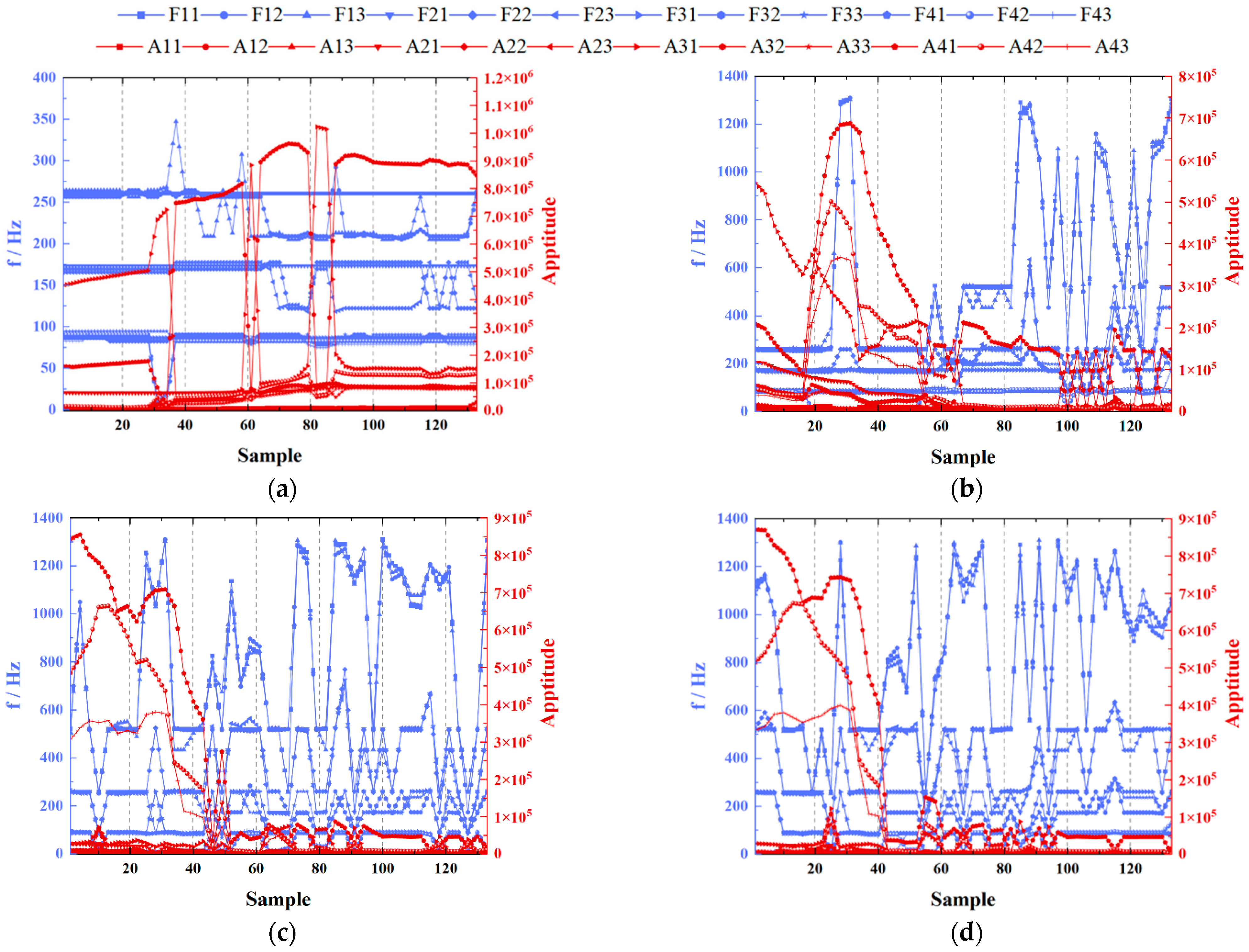
Figure 19 illustrates the feature value distribution changes for the 133 numerical simulation samples. This figure allows for a detailed comparison of the feature representation capabilities of the simulated pressure fluctuation signals from different measurement points in capturing the cavitation degree of the axial flow pump.

Figure 19. Distribution of IMFs characteristic values for 133 numerical simulation samples at different monitoring points: (a) Measurement point M1; (b) Measurement point M2; (c) Measurement point M3; (d) Measurement point M4.

As shown in Figure 19a, the IMF frequency distribution at M1 is relatively stable compared to other measurement points, suggesting that the feature values from the M1 pressure fluctuation signals have weaker representational power for the cavitation degree, making it less suitable as an input for the model. Figure 19b shows that the feature values from the signal decomposition at M2 exhibit larger fluctuations, with higher discriminability between different samples. Since M2 is close to the inlet of the guide vanes, which are more significantly affected by cavitation in the impeller region, the data from M2 is more suitable as an input for the VMD-SWO-BiLSTM model. Similarly, Figure 19c,d demonstrate that the signal feature values from M3 and M4 also have good discriminability.

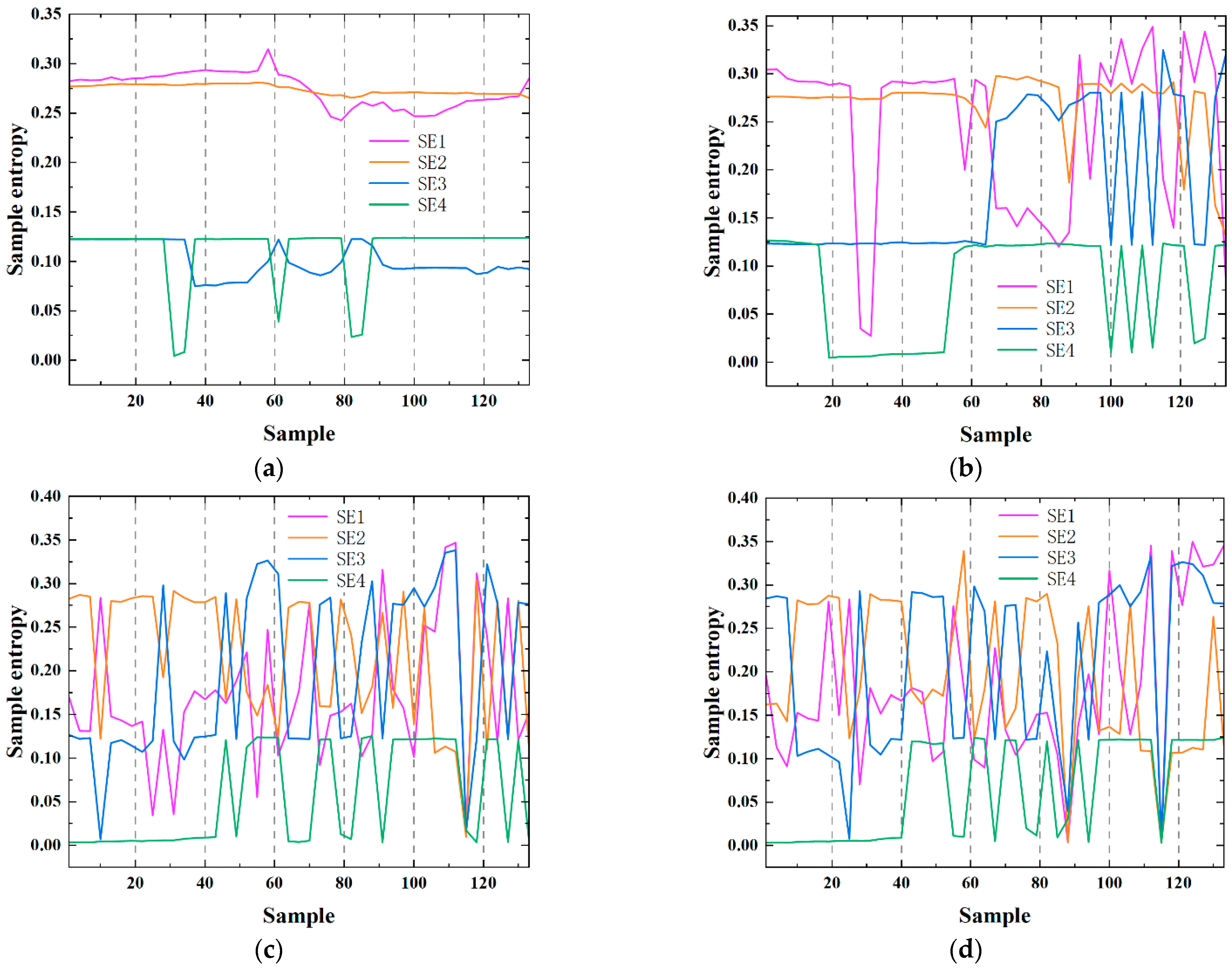
Figure 20 compares the sample entropy (SE) results of the IMFs for the four measurement points’ simulated signals after VMD. SE1 represents the sample entropy of the IMF1 time series, SE2 represents the sample entropy of the IMF2 time series, SE3 represents the sample entropy of the IMF3 time series, and SE4 represents the sample entropy of the IMF4 time series.

Figure 20. Distribution of IMFs sample entropy values for different samples at four monitoring points: (a) Measurement point M1; (b) Measurement point M2; (c) Measurement point M3; (d) Measurement point M4.

As shown in Figure 20, for all the samples in this study, the sample entropy values for M3 and M4 show significant variation, indicating that the IMFs at these two measurement points lack regularity in their sample distribution. The sample entropy at M2 shows substantial variation in the cavitation development stage samples, while the IMFs’ sample entropy at M1 has the smallest variation among the four measurement points. Combining the pressure fluctuation feature value distribution, it is evident that M2, M3, and M4 have better discriminability in their pressure fluctuation signal features, with M4 located at the discharge elbow, farther from the impeller, and showing a similar feature distribution to M3. Therefore, the signal feature values from M2 and M3 are selected as inputs for the model, while also considering the influence of measurement point input combinations on the model’s prediction results.

6.2. Model Identification Results

In this study, 133 samples from the dataset were randomly shuffled, and the Hold-Out method [38] was employed to divide the disordered samples into a training set and a testing set. Specifically, the first 93 samples were used as the training set, and the remaining 40 samples as the testing set. Considering different sensor input configurations, the VMD-SWO-BiLSTM model was applied to identify the cavitation coefficient. Additionally, in light of the relatively small sample size in this study, K-fold cross-validation [39] was adopted to train the VMD-SWO-BiLSTM model, and the identification results were compared with those obtained from the Hold-Out method. In K-fold cross-validation, the entire dataset is divided into K subsets of approximately equal size. In this study, the data were divided into 7 folds, with each fold containing 19 samples. Each subset was used once as the validation set, while the remaining six subsets were used for training, resulting in a total of 7 training iterations. The intermediate layer weights of the neural network obtained from each training iteration were then averaged to form the final model. To further address concerns related to limited sample size, confidence intervals and standard deviations of the identification errors were calculated for each competing model. In addition, a statistical significance test based on the paired t-test was conducted to compare model performance under identical data splits. The results demonstrated that the VMD-SWO-BiLSTM model achieved significantly lower prediction errors (p < 0.05) than the benchmark models, confirming that the performance improvement is statistically meaningful rather than due to random variation in the small dataset. 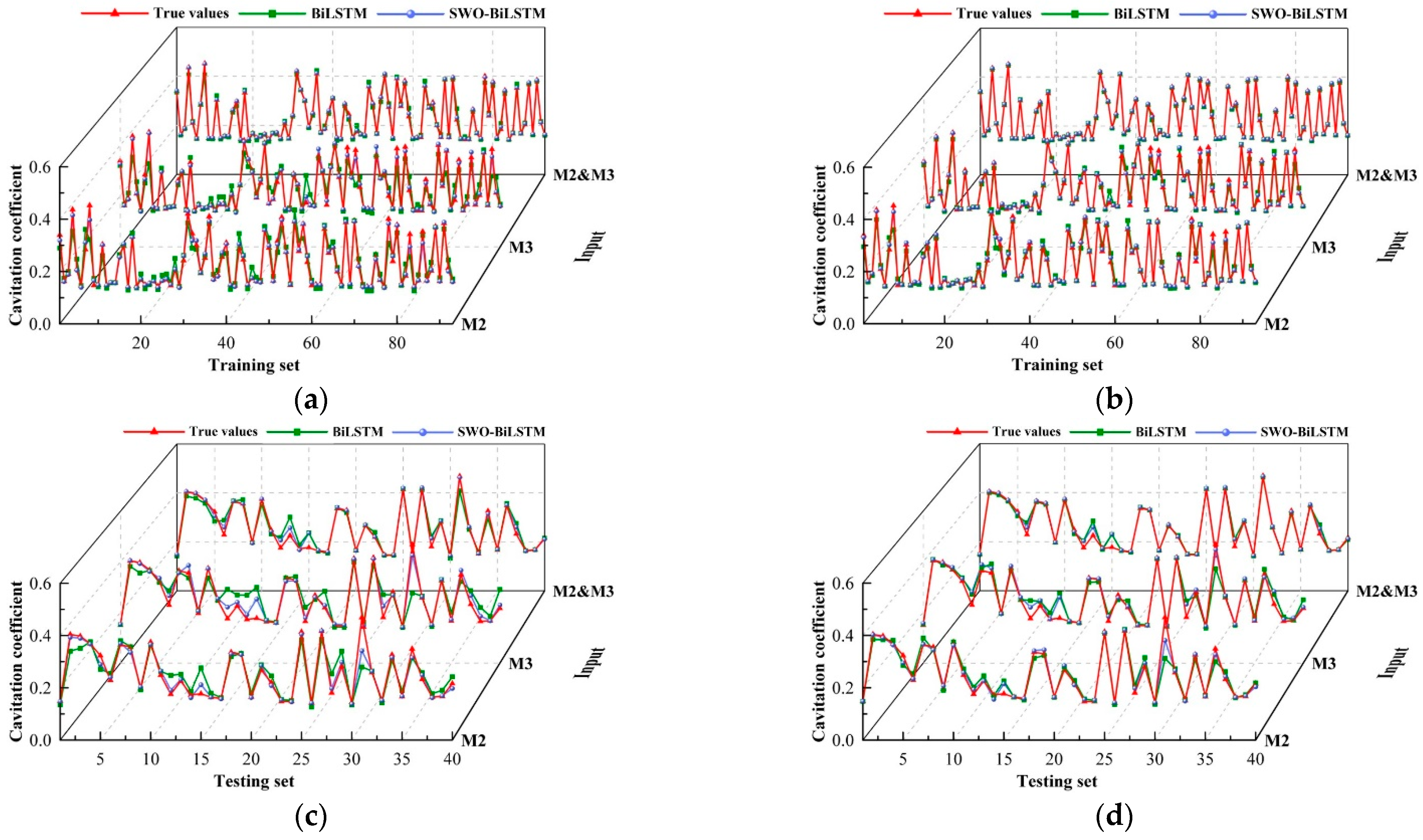Figure 21 presents the identification results of both the BiLSTM and VMD-SWO-BiLSTM models under the two sample partitioning strategies.

Figure 21. Cavitation coefficient identification results of the BiLSTM and VMD-SWO-BiLSTM models under two data-partitioning strategies: (a) Training set identification results using the Hold-Out method; (b) Training set identification results using K-fold cross-validation; (c) Test set identification results using the Hold-Out method; (d) Test set identification results using K-fold cross-validation.

According to Figure 21, the model achieves better prediction accuracy on the training set than on the testing set, which is expected, as model parameter learning is based on the training data. Comparing Figure 21a,b, the training set prediction results under both partitioning methods show no significant difference, thus requiring quantitative comparison using error metrics. In contrast, the testing set results shown in Figure 21c,d demonstrate that the K-fold cross-validation method yields more accurate predictions than the Hold-Out method. This indicates that K-fold cross-validation is more effective for model training when the sample size is limited, as it allows for more comprehensive utilization of available data, thereby improving model performance. Moreover, in comparison to the BiLSTM model, the proposed SWO-BiLSTM model provides predictions that are closer to the actual values of the cavitation coefficient, indicating that SWO is effective in optimizing model hyperparameters and enhancing the model’s prediction capability. From the comparison across the four subfigures, it is evident that using the pressure fluctuation features from both M2 and M3 sensors as a combined input results in predictions that more closely match the actual cavitation coefficients. In order to quantitatively compare these results, a prediction performance evaluation is necessary.

6.3. Model Performance Evaluation

As discussed in Section 6.1, to evaluate the impact of different sensor locations and combinations on the prediction performance of cavitation coefficient identification, as well as to compare the predictive capability of the SWO-BiLSTM model with that of the unoptimized BiLSTM model, this study adopts Root Mean Square Error (RMSE), Mean Absolute Error (MAE), Mean Absolute Percentage Error (MAPE), Mean Squared Error (MSE) and the coefficient of determination (R²) as the performance evaluation metric for models [40]. The formulas for these metrics are provided in Table 4.

Table 4. Algorithm performance evaluation metrics.

Eigenvalue	Formulas
MAE	$\mathrm{MAE}={\displaystyle \frac{1}{n}}{\sum }_{i=1}^n|y_i-{\hat{y}}_i|$
MAPE	$\mathrm{MAPE}={\displaystyle \frac{1}{n}}{\sum }_{i=1}^n\left|{\displaystyle \frac{y_i-{\hat{y}}_i}{y_i}}\right|\times 100\%$
MSE	$\mathrm{MSE}={\displaystyle \frac{1}{n}}{\sum }_{i=1}^n(y_i-{\hat{y}}_i{)}^2$
RMSE	$\mathrm{RMSE}=\sqrt{{\displaystyle \frac{1}{n}}{\sum }_{i=1}^n(y_i-{\hat{y}}_i{)}^2}$
$1-R^2$	$1-{\mathrm{R}}^2={\displaystyle \frac{{\sum }_{i=1}^n(y_i-{\hat{y}}_i{)}^2}{{\sum }_{i=1}^n(y_i-\bar{y}{)}^2}}$

Where n is the total number of samples, $y_i$ is the predicted value, and $\widehat{y_i}$ is the actual value.

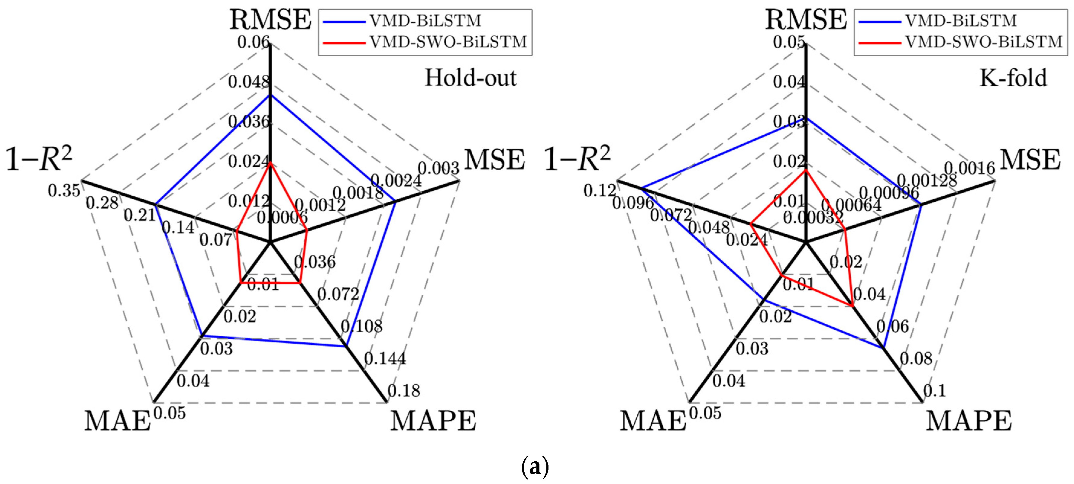
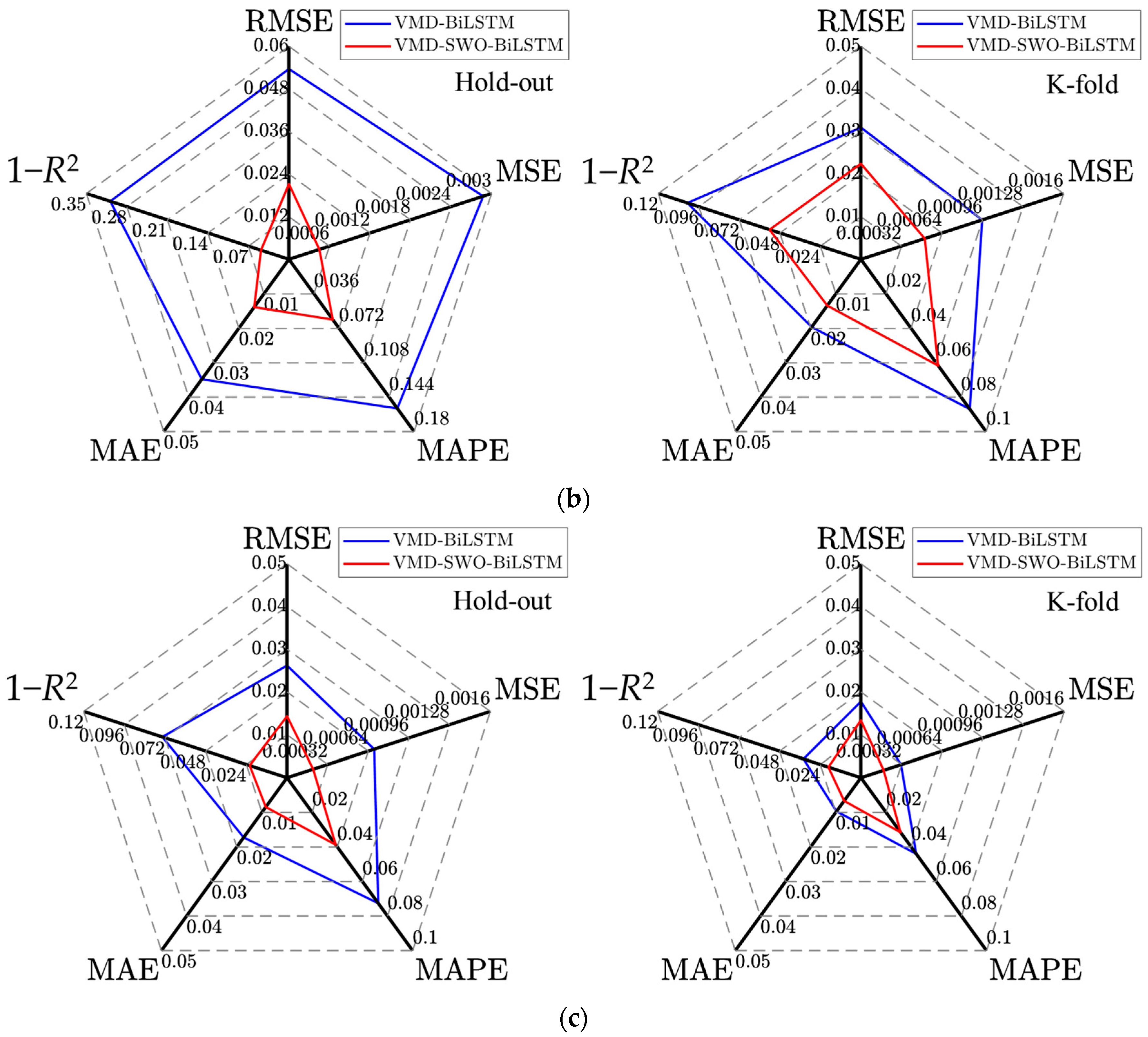
Figure 22 presents the identification performance evaluation results on the test set under single-point and combined-input conditions for M2 and M3 sensor data.

Figure 22. Evaluation of test set identification results using different input configurations. (a) Single-point input at M2; (b) Single-point input at M3; (c) Combined input from M2 and M3.

As shown in Figure 22, the proposed VMD-SWO-BiLSTM model consistently outperforms the VMD-BiLSTM model under both Hold-out and K-fold cross-validation, as well as under all input configurations. Across different measurement-point inputs, the 1 − R² values of the VMD-SWO-BiLSTM model remain within 0–0.07, while the remaining evaluation metrics are close to zero, indicating excellent predictive accuracy. This improvement stems from the ability of the SWO algorithm to achieve an effective balance between global exploration and local exploitation, thereby avoiding premature convergence and enhancing the robustness of hyperparameter optimization. Consequently, the VMD-SWO-BiLSTM model exhibits noticeably stronger identification capability than the baseline VMD-BiLSTM model. A comparison of Figure 22a–c further shows that using combined signals from measurement points M2 and M3 yields higher identification accuracy for both models compared with single-point inputs. Under this combined-input configuration, the VMD-SWO-BiLSTM model achieves a 1 − R² value of 0.0192 and MAPE values below 5%, demonstrating its strong and reliable performance in cavitation-coefficient identification.

6.4. Experimental Data Validation

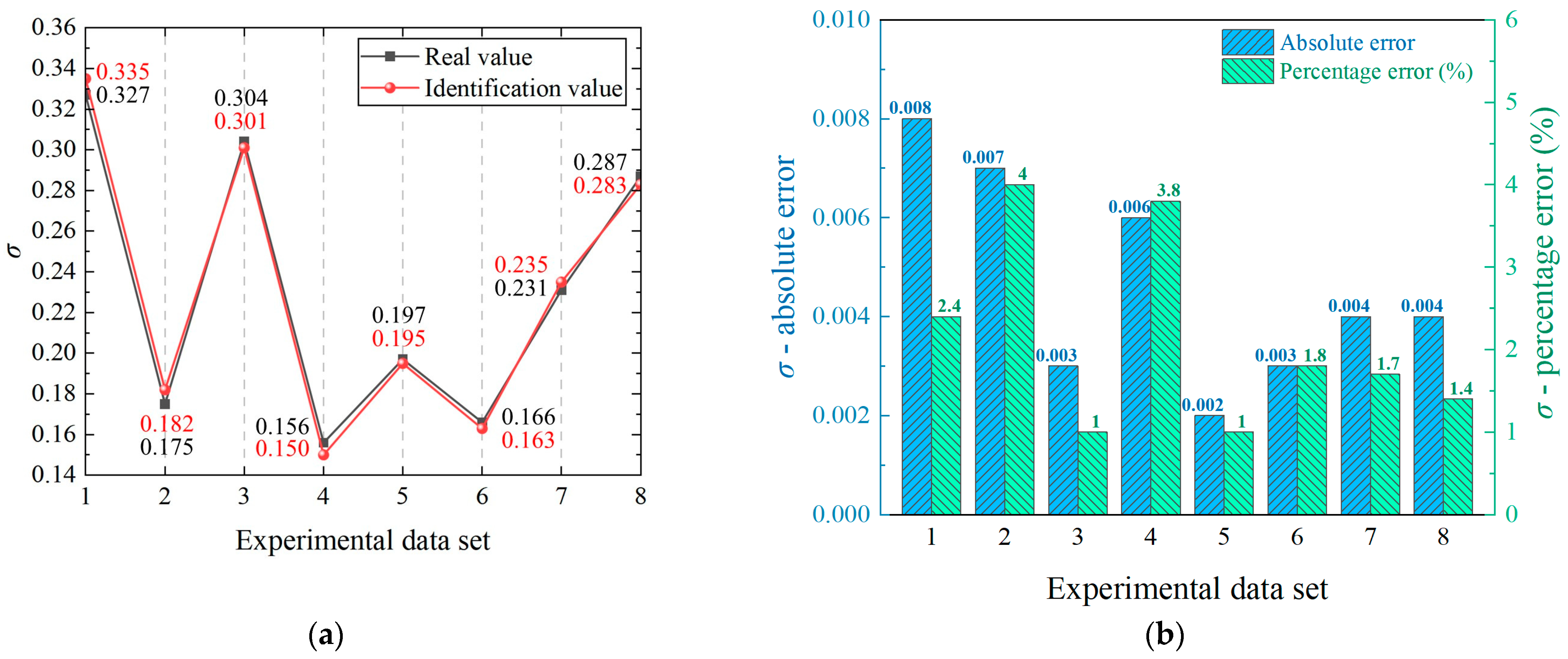
To evaluate the performance of the proposed SWO-BiLSTM model for cavitation coefficient identification in practical scenarios, this study utilized eight sets of experimental data samples for validation. First, feature extraction was conducted on the pressure fluctuation signals obtained from measurement points M2 and M3. The resulting feature matrices were then input into the pre-trained SWO-BiLSTM model for cavitation coefficient identification. The identification results are shown in Figure 23a, while Figure 23b presents the absolute error and percentage error of the identified results.

Figure 23. Validation of the proposed VMD-SWO-BiLSTM model using experimental data: (a) Cavitation coefficient identification results for eight experimental samples; (b) Absolute and percentage identification errors.

Figure 23a indicates that the cavitation coefficient identification results obtained using the proposed SWO-BiLSTM model exhibit a high degree of agreement with the true values. According to the error comparison shown in Figure 23b, the maximum absolute error in the identified cavitation coefficients is 0.008, and the maximum percentage error is 4%, which is less than 5%. These results demonstrate the reliability of the proposed identification method.

7. Conclusions

This study proposes an innovative machine learning model for the identification of the cavitation coefficient in axial flow pumps, integrating Variational Mode Decomposition (VMD), Sample Entropy, the Spider Wasp Optimization (SWO) algorithm, and Bidirectional Long Short-Term Memory (BiLSTM) networks, forming a composite VMD-SWO-BiLSTM framework. The model is trained using multi-point pressure fluctuation signal features obtained from unsteady internal flow simulations of the pump device. Its performance is systematically evaluated and validated, confirming its accuracy. The main conclusions are as follows:

(1)

The proposed VMD-SWO-BiLSTM model significantly outperforms the conventional VMD-BiLSTM model in cavitation coefficient identification accuracy. Across different measurement-point inputs, the 1 − R² values of the VMD-SWO-BiLSTM model remain within 0–0.07, while the remaining evaluation metrics are close to zero, indicating excellent identification accuracy. Under limited data conditions, compared to training via the Hold-out sample partitioning method, the VMD-SWO-BiLSTM model further improves its recognition accuracy within the K-fold cross-validation framework. The results demonstrate the effectiveness of the SWO algorithm in optimizing model hyperparameters and notably enhance both recognition performance and adaptability, providing a novel and efficient tool for precise cavitation diagnostics.

(2)

In the context of cavitation coefficient identification for axial flow pumps, the use of multi-point combined feature inputs shows clear advantages in improving accuracy and model stability. Compared with single-point input, using combined inputs yields higher identification accuracy for both VMD-BiLSTM and VMD-SWO-BiLSTM models. Under this combined-input configuration, the VMD-SWO-BiLSTM model achieves a 1 − R² value of 0.0192 and MAPE values below 5%. These findings confirm that the proposed model and approach offer high accuracy and practical applicability in complex, multi-sensor environments.

(3)

Validation using eight sets of experimental data shows that the cavitation coefficient predictions of the SWO-BiLSTM model align closely with actual values. The maximum absolute error is only 0.006, and the maximum percentage error is 4.7%, both well within the 5% threshold. This further confirms the reliability and engineering applicability of the proposed VMD-SWO-BiLSTM model, offering an effective new pathway for online monitoring and intelligent diagnosis of cavitation conditions in axial flow pumps and other hydraulic machinery.

Although the proposed VMD-SWO-BiLSTM framework demonstrates strong accuracy and robustness in identifying cavitation coefficients, several limitations should be acknowledged. The dataset size is relatively small, and sensitivity analysis of cavitation model parameters was not considered in the present study. In addition, the model proposed in this study is based on axial-flow pumps and does not consider other types of pumps. In future work, larger experimental datasets covering broader operating conditions will be collected to further enhance model generalization. Additionally, integrating multi-source signals, exploring other physics-informed neural network structures, and developing real-time online monitoring systems will be valuable directions. These efforts will help expand the applicability of the proposed method to more complex hydraulic machinery.